Embed Size (px)
Citation preview
Title: 1
Summer temperature regimes in southcentral Alaska streams: watershed drivers of variation and 2
potential implications for Pacific salmon 3
4
5
Authors: 6
Sue Mauger1, Rebecca Shaftel
2, Jason Leppi
3, Daniel Rinella
2, 4, 5 7
8
1Cook Inletkeeper, 3734 Ben Walters Lane, Homer, AK 99603, [email protected] 9
10
2Alaska Center for Conservation Science, University of Alaska Anchorage, 3211 Providence Dr., 11
Anchorage, AK 99508, [email protected] 12
13
3The Wilderness Society, 705 Christensen Dr., Anchorage, AK 99501, [email protected] 14
15
4Department of Biological Sciences, University of Alaska Anchorage, 3211 Providence Dr., Anchorage, AK 16
99508 17
18
5Current address: U.S. Fish and Wildlife Service, Anchorage Conservation Office, 4700 BLM Road, 19
Anchorage, AK 99507; [email protected] 20
21
Corresponding author: 22
Sue Mauger, 3734 Ben Walters Lane, Homer, AK 99603, 907-235-4068 x24, 907-235-4069, 23
Page 1 of 48C
an. J
. Fis
h. A
quat
. Sci
. Dow
nloa
ded
from
ww
w.n
rcre
sear
chpr
ess.
com
by
UN
IVE
RSI
TY
OF
AL
ASK
A A
NC
HO
RA
GE
on
10/3
1/16
For
pers
onal
use
onl
y. T
his
Just
-IN
man
uscr
ipt i
s th
e ac
cept
ed m
anus
crip
t pri
or to
cop
y ed
iting
and
pag
e co
mpo
sitio
n. I
t may
dif
fer
from
the
fina
l off
icia
l ver
sion
of
reco
rd.
Abstract 25
26
Climate is changing fastest in high latitude regions, focusing our research on understanding rates and 27
drivers of changing temperature regimes in southcentral Alaska streams and implications for salmon 28
populations. We collected continuous water and air temperature data during open-water periods from 29
2008 to 2012 in 48 non-glacial salmon streams across the Cook Inlet basin spanning a range of 30
watershed characteristics. The most important predictors of maximum temperatures, expressed as 31
mean July temperature, maximum weekly average temperature, and maximum weekly maximum 32
temperature (MWMT), were mean elevation and wetland cover, while thermal sensitivity (slope of the 33
stream-air temperature relationship) was best explained by mean elevation and area. Although 34
maximum stream temperatures varied widely (8.4 to 23.7 oC) between years and across sites, MWMT at 35
most sites exceeded established criterion for spawning and incubation (13 oC), above which chronic and 36
sub-lethal effects become likely, every year of the study, which suggests salmon are already 37
experiencing thermal stress. Projections of MWMT over the next ~50 years suggest these criteria will be 38
exceeded at more sites and by increasing margins. 39
40
Keywords: stream temperature, climate change, Pacific salmon, Cook Inlet, Alaska 41
Page 2 of 48C
an. J
. Fis
h. A
quat
. Sci
. Dow
nloa
ded
from
ww
w.n
rcre
sear
chpr
ess.
com
by
UN
IVE
RSI
TY
OF
AL
ASK
A A
NC
HO
RA
GE
on
10/3
1/16
For
pers
onal
use
onl
y. T
his
Just
-IN
man
uscr
ipt i
s th
e ac
cept
ed m
anus
crip
t pri
or to
cop
y ed
iting
and
pag
e co
mpo
sitio
n. I
t may
dif
fer
from
the
fina
l off
icia
l ver
sion
of
reco
rd.
Introduction 42
43
Climate is changing fastest in high latitude regions like Alaska, where average annual air temperature 44
has increased nearly 2 °C over the past 50 years and is projected to rise by an additional ~2–4 °C in 45
coming decades (Karl et al. 2009). This warming is associated with ongoing, interrelated changes in the 46
hydrologic and temperature regimes of Alaska’s fresh waters (Prowse et al. 2006), such as earlier ice 47
breakup (Schindler et al. 2005, U.S. EPA 2015), earlier depletion of snowmelt-derived streamflow 48
(Stewart et al. 2005), and increasing water temperature (Taylor 2008). 49
50
The effects of water temperature on Pacific salmon (Oncorhynchus spp.) are pervasive. The abundance 51
and taxonomic composition of prey and the seasonal timing of its availability are closely linked with 52
temperature regimes (Caissie 2006; Burgmer et al. 2007). Physiological growth potential increases to an 53
optimum temperature and declines as temperature increases (Brett et al. 1969). Timing of life history 54
events, like spawning, emergence and the onset of exogenous feeding, and smolting, are adapted to 55
prevailing environmental conditions and are largely driven by temperature (Brannon 1987, Quinn 2005). 56
High temperatures can block migration corridors (Quinn et al. 1997, Salinger and Anderson 2006), 57
increase disease virulence (Fryer and Pilcher 1974, Kocan et al. 2009), and cause stress or outright death 58
(Richter and Kolmes 2006). As such, warming temperature has the potential to alter the suitability of 59
waterbodies for salmon populations. 60
61
Anticipating the magnitude and scope of ecological changes to freshwater habitats is essential for the 62
management of Alaska’s salmon populations, which contribute substantially to global wild salmon 63
production (Ruggerone et al. 2010) and are exceedingly important to Alaska’s ecology, economy, and 64
societal well-being. Despite the rapidly warming climate, and recent studies projecting decreases in 65
Page 3 of 48C
an. J
. Fis
h. A
quat
. Sci
. Dow
nloa
ded
from
ww
w.n
rcre
sear
chpr
ess.
com
by
UN
IVE
RSI
TY
OF
AL
ASK
A A
NC
HO
RA
GE
on
10/3
1/16
For
pers
onal
use
onl
y. T
his
Just
-IN
man
uscr
ipt i
s th
e ac
cept
ed m
anus
crip
t pri
or to
cop
y ed
iting
and
pag
e co
mpo
sitio
n. I
t may
dif
fer
from
the
fina
l off
icia
l ver
sion
of
reco
rd.
suitable habitat for Pacific salmonids elsewhere (Morrison et al. 2002, Isaak et al. 2011, Ruesch et al. 66
2012, Jones et al. 2013), researchers are just beginning to understand rates and drivers of changing 67
temperature regimes in Alaska streams and the implications for salmon (e.g., see Kyle and Brabets 2001, 68
Davis and Davis 2008, Lisi et al. 2013, Fellman et al. 2014, Leppi et al. 2014, Wobus et al. 2015). 69
70
Regional analyses conducted outside of Alaska have relied on the compilation and synthesis of extensive 71
data collected by multiple agencies and organizations over the last few decades (e.g. Isaak et al. 2010, 72
Mantua et al. 2010). Long-term stream temperature datasets and regional monitoring networks in 73
Alaska are limited, likely due to the minimal need for restoration planning in Alaska’s relatively intact 74
watersheds and relatively cool climate toward the northern end of Pacific salmon distribution. 75
However, interest in developing stream and lake monitoring networks across Alaska is growing because 76
a coordinated monitoring approach can generate regional-scale data useful for prioritizing sensitive 77
areas for conservation and targeting other management strategies that can increase resiliency in aquatic 78
ecosystems to a changing climate (Reynolds et al. 2013). 79
80
Summer stream temperature regimes, and the sensitivity of streams to climatic warming, are influenced 81
by climate, landscape features, and characteristics of the stream and its channel (Mayer 2012). For the 82
non-glacial salmon streams examined in this study, we expected the warmest and most thermally 83
sensitive streams to drain low-elevation landscapes with features that enhance opportunities for 84
absorption of solar radiation and equilibration to air temperature, such as low valley slope, large 85
watershed area, and relatively high cover of wetlands, standing water, and non-forested areas (Caissie 86
2006, Lisi et al. 2013). We anticipated that lakes would have a warming, rather than moderating, effect 87
on summer stream temperatures (Jones 2010, Lisi et al. 2013), particularly because lakes drained by our 88
study streams tend to be shallow and dark-bottomed. However, we expected that higher streamflow, 89
Page 4 of 48C
an. J
. Fis
h. A
quat
. Sci
. Dow
nloa
ded
from
ww
w.n
rcre
sear
chpr
ess.
com
by
UN
IVE
RSI
TY
OF
AL
ASK
A A
NC
HO
RA
GE
on
10/3
1/16
For
pers
onal
use
onl
y. T
his
Just
-IN
man
uscr
ipt i
s th
e ac
cept
ed m
anus
crip
t pri
or to
cop
y ed
iting
and
pag
e co
mpo
sitio
n. I
t may
dif
fer
from
the
fina
l off
icia
l ver
sion
of
reco
rd.
through the thermal mass it affords (Caissie 2006, Kelleher et al. 2012), and permeable landscapes 90
conducive to the recharge and discharge of groundwater (O’Driscoll and DeWalle 2006, Chang and Psaris 91
2013, Johnson et al. 2013) would act to moderate water temperature and thermal sensitivity. 92
93
Our research focused on answering the following questions related to summer temperature regimes, 94
specifically thermal maxima and thermal sensitivity, in salmon streams of the Cook Inlet region, 95
southcentral Alaska: 96
1) How do temperature regimes vary among streams and years? 97
2) How are temperature regimes related to site and watershed characteristics and site-specific air 98
temperature? 99
3) What are the potential implications of these temperature regimes for different salmon species 100
and life stages now and in the future? 101
102
Methods 103
104
Study area and temperature monitoring 105
This work focused on non-glacial salmon streams in southcentral Alaska’s Cook Inlet basin (Fig. 1). Cook 106
Inlet opens southward to the Gulf of Alaska and its basin (121,700 km2) consists of coastal and valley 107
lowlands surrounded by rugged mountains, including some of North America’s highest peaks. The 108
climate ranges from continental to maritime, with mean annual temperatures between -6 and 6 oC 109
(Brabets 1999). Precipitation, much of which falls as snow during winter months, ranges annually from 110
50 cm across the continental zone to 180 cm across the maritime zone, with the greatest amounts 111
falling in mountainous areas (Brabets 1999). The basin’s major river systems drain alpine glaciers and 112
therefore have high sediment loads and turbidity (Lloyd et al. 1987), although many of the tributary 113
Page 5 of 48C
an. J
. Fis
h. A
quat
. Sci
. Dow
nloa
ded
from
ww
w.n
rcre
sear
chpr
ess.
com
by
UN
IVE
RSI
TY
OF
AL
ASK
A A
NC
HO
RA
GE
on
10/3
1/16
For
pers
onal
use
onl
y. T
his
Just
-IN
man
uscr
ipt i
s th
e ac
cept
ed m
anus
crip
t pri
or to
cop
y ed
iting
and
pag
e co
mpo
sitio
n. I
t may
dif
fer
from
the
fina
l off
icia
l ver
sion
of
reco
rd.
streams and smaller watersheds have little or no glacial influence and are clear. Cook Inlet basin has 114
12,000 km of documented salmon streams and supports substantial wild runs of all five North American 115
Pacific salmon plus other anadromous and resident fishes (Johnson and Coleman 2014). The basin’s 116
salmon populations are harvested in commercial, personal use, subsistence, and sport fisheries. Most of 117
the basin is free from anthropogenic watershed disturbances, although urban and suburban 118
development occurs around Anchorage (Alaska’s largest city) and several smaller communities which, 119
collectively, are home to more than two thirds of Alaska’s human population. 120
121
We monitored water temperature in 48 non-glacial salmon streams across the basin (Fig. 1) spanning a 122
range of watershed characteristics (Table 1), and in most cases, could be accessed by the region’s sparse 123
road network. We focused on non-glacial streams because they tend to be warmer during summer than 124
those that receive glacial meltwater (Kyle and Brabets 2001, Fellman et al. 2014) and thus likely more 125
susceptible to thermal change over the next 50 years. Water temperature in the larger glacial systems 126
of the region may be buffered in the short-term as monthly streamflows are projected to increase 127
through the mid-21st century (Debjani et al. 2015). We established one temperature monitoring site in 128
the lowest accessible reach of each stream's watershed; 22 of the streams flow directly to the ocean (all 129
sites on these streams are within 5 km of Cook Inlet), 23 streams flow into glacial river systems, and 130
three streams flow into another non-glacial system. With only one site per watershed, we did not 131
expect to capture the spatial heterogeneity of water temperature and cold-water refugia within each 132
watershed; instead, our sampling approach allowed us to identify characteristics that influence 133
cumulative stream temperature patterns and describe temperature heterogeneity at a regional scale. 134
135
All 48 streams are listed in the Alaska Department of Fish and Game’s Anadromous Waters Catalog 136
(Johnson and Coleman 2014), with Coho salmon (Oncorhynchus kisutch) being the most widespread 137
Page 6 of 48C
an. J
. Fis
h. A
quat
. Sci
. Dow
nloa
ded
from
ww
w.n
rcre
sear
chpr
ess.
com
by
UN
IVE
RSI
TY
OF
AL
ASK
A A
NC
HO
RA
GE
on
10/3
1/16
For
pers
onal
use
onl
y. T
his
Just
-IN
man
uscr
ipt i
s th
e ac
cept
ed m
anus
crip
t pri
or to
cop
y ed
iting
and
pag
e co
mpo
sitio
n. I
t may
dif
fer
from
the
fina
l off
icia
l ver
sion
of
reco
rd.
(documented in 47 streams) followed by Pink salmon (Oncorhynchus gorbuscha, 36 streams), Chinook 138
salmon (Oncorhynchus tshawytscha, 34 streams), Sockeye salmon (Oncorhynchus nerka, 31 streams) 139
and Chum salmon (Oncorhynchus keta, 23 streams). In 44 streams the temperature monitoring site was 140
located in documented spawning habitat for one or more salmon species, while all but one had 141
documented spawning habitat upstream of the monitoring station (Johnson and Coleman 2014). 142
Locations (latitude/longitude) and stream names for all sites are provided in Table S1. 143
144
From 2008 to 2012, we deployed paired water and air temperature loggers programmed to record at 145
15- or 30-minute intervals starting mid-May to mid-June, as conditions allowed, and collected them 146
after October 1 (see Mauger 2008 for more details). For water temperature, we secured HOBO Pro v2 147
and StowAway TidbiT data loggers (Onset Computer Corporation, Bourne, Massachusetts) in well-mixed 148
locations within the water column of the mainstem channel to minimize the influence of direct 149
groundwater connection or other reach-scale dynamics. For air temperature, we placed a data logger 150
within a solar shield and secured it 8-30 meters away from the stream and at least 1.8 meters off the 151
ground. Our five years of open-water sampling captured a period comparable to or slightly colder than 152
the most recent 35 years in the Cook Inlet region (NOAA 2015). The regional summertime temperature 153
anomaly (June–August mean temperature difference from 1980-2014 baseline) ranged from -1.1 oC to 154
+0.3 oC, with 2009 being the warmest year of the study period. 155
156
We checked data loggers against a NIST (National Institute of Standards and Technology) thermometer 157
before and after each deployment in 0 and 20 o
C water baths to ensure we met our 0.25 o
C accuracy 158
goal. We reviewed downloaded logger data and deleted erroneous measurements following Mauger et 159
al. (2015). We attempted to collect five years of stream and air temperature data at 48 sites, thus 160
potentially generating 240 “site-years” of data; however, data for 24 site-years were not collected due 161
Page 7 of 48C
an. J
. Fis
h. A
quat
. Sci
. Dow
nloa
ded
from
ww
w.n
rcre
sear
chpr
ess.
com
by
UN
IVE
RSI
TY
OF
AL
ASK
A A
NC
HO
RA
GE
on
10/3
1/16
For
pers
onal
use
onl
y. T
his
Just
-IN
man
uscr
ipt i
s th
e ac
cept
ed m
anus
crip
t pri
or to
cop
y ed
iting
and
pag
e co
mpo
sitio
n. I
t may
dif
fer
from
the
fina
l off
icia
l ver
sion
of
reco
rd.
to loggers being lost during high flow events or other deployment failures. In addition, we removed 17 162
site-years due to missing or problematic local air temperature data and nine site-years due to 163
deployment periods that likely missed the thermal maxima. The final dataset included 48 sites with 1-5 164
years of data totaling 190 site-years of stream and air temperature data. Deployment dates spanned at 165
least June 16 – August 31 for 168 sites-years, with 22 sites-years having shorter deployment periods 166
which we evaluated to have captured the thermal maxima. 167
168
Stream temperature metrics 169
We aggregated the quality-controlled stream and air temperature time series for all days with at least 170
90% of daily measurements into daily means and maximums, which we then used to calculate 171
temperature metrics. We selected three metrics to describe aspects of the summer temperature 172
regimes in the 48 streams: mean July temperature, maximum weekly average temperature (MWAT), 173
and maximum weekly maximum temperature (MWMT). We chose mean July stream temperature 174
because this is typically the hottest month in southcentral Alaska. We calculated mean July temperature 175
only for site-years when at least 90% of the days were captured (>27 days). We used MWAT and 176
MWMT because they represent an intermediate time period over which transient high temperatures 177
may affect fitness in aquatic organisms. We calculated MWAT by selecting the maximum from a weekly 178
(7-day rolling) average of mean daily stream temperatures and calculated MWMT by selecting the 179
maximum from a weekly (7-day rolling) average of maximum daily stream temperatures across the 180
entire deployment period. All three of these temperature metrics have been useful for describing 181
relative differences in thermal maxima between streams and potential impacts to salmonids (Wehrly et 182
al. 2009, Isaak et al. 2010, Ruesch et al. 2012, Moore et al. 2013). 183
184
Page 8 of 48C
an. J
. Fis
h. A
quat
. Sci
. Dow
nloa
ded
from
ww
w.n
rcre
sear
chpr
ess.
com
by
UN
IVE
RSI
TY
OF
AL
ASK
A A
NC
HO
RA
GE
on
10/3
1/16
For
pers
onal
use
onl
y. T
his
Just
-IN
man
uscr
ipt i
s th
e ac
cept
ed m
anus
crip
t pri
or to
cop
y ed
iting
and
pag
e co
mpo
sitio
n. I
t may
dif
fer
from
the
fina
l off
icia
l ver
sion
of
reco
rd.
As a fourth response variable, we calculated thermal sensitivity for all sites with at least 3 years of 185
stream and air temperature data (n=45), which we expressed as the slope of the stream-air temperature 186
relationship (Kelleher et al. 2012, Mayer 2012, Chang and Psaris 2013, Luce et al. 2014) based on weekly 187
average temperatures during July. Although others have shown the stream-air relationship to flatten 188
out at high air temperatures (>20 oC) due to the effect of evaporative cooling (Mohseni et al. 1998, 189
Mayer 2012), southcentral Alaska’s air temperatures in July rarely exceed 20 oC. Because streams in 190
colder climates do not show a significant change of slope at these moderate air temperatures (Mohseni 191
and Stefan 1999), we chose to use a linear relationship. We selected weekly measurements over daily 192
because the relationship between stream and air temperatures becomes stronger as the time scale 193
increases (Erickson and Stefan 2000). We used a linear mixed effects model with a random intercept for 194
year to account for the temporal correlation between weekly values within a year. We used Akaike's 195
Information Criterion to compare results from a mixed effects model to one without a random 196
intercept; the mixed effects model resulted in better model fit at 29 of the 48 sites. The slopes from the 197
mixed effects model were generally lower than the slopes from the fixed effects model (37 of 48 sites), 198
which we hypothesized was due to the variable influence of snowmelt on stream temperatures during 199
July in some streams. 200
201
In addition to the temperature metrics described above, we calculated overall maximum temperature; 202
weekly and monthly average, maximum, and minimum temperature; daily minimum temperature; and 203
maximum daily fluctuation for each site-year (Table S2). 204
205
Independent predictors of water temperature: site, watershed, and air temperature 206
We generated a suite of 12 site or watershed characteristics that we hypothesized directly or indirectly 207
affect stream temperatures. Land-cover statistics (percent wetlands, forested, and open water) were 208
Page 9 of 48C
an. J
. Fis
h. A
quat
. Sci
. Dow
nloa
ded
from
ww
w.n
rcre
sear
chpr
ess.
com
by
UN
IVE
RSI
TY
OF
AL
ASK
A A
NC
HO
RA
GE
on
10/3
1/16
For
pers
onal
use
onl
y. T
his
Just
-IN
man
uscr
ipt i
s th
e ac
cept
ed m
anus
crip
t pri
or to
cop
y ed
iting
and
pag
e co
mpo
sitio
n. I
t may
dif
fer
from
the
fina
l off
icia
l ver
sion
of
reco
rd.
derived for each watershed from 30-meter resolution LANDSAT imagery (1999, 2003). Maximum 209
watershed elevation, mean watershed elevation, logger site elevation, mean watershed slope, and 210
watershed area, were derived from the U.S. Geological Survey (USGS) National Elevation Dataset 2-arc-211
second (about 60-meter grid spacing) Digital Elevation Model (DEM). The 60-meter DEM was chosen 212
because it had seamless coverage of the project area. Stream gradient was derived from the USGS 213
National Hydrography Dataset (NHD). Lake influence was calculated for 23 watersheds with lakes larger 214
than 0.5 km2 connected to the stream network. The area for each lake (n=51) was divided by its 215
distance to the monitoring site to generate an inverse-distance weighted lake effect and summed across 216
each watershed since some sites had more than one lake in their watershed. As a proxy for aquifer 217
permeability and groundwater contribution to streams, we calculated the percent unconsolidated fluvial 218
surficial geology (Wilson et al. 2012). Mean annual discharge was calculated using a regression equation 219
developed for southcentral Alaska based on watershed area and mean annual precipitation (Verdin 220
2004); mean annual precipitation inputs to the equation were based on an average for the years 1980-221
2009 (SNAP 2014). Watersheds for each site were delineated by manually editing the watershed 222
boundary dataset (6th level Hydrologic Unit Codes) and all watershed attributes were developed using 223
ArcGIS 10.1. 224
225
In addition to site and watershed predictors, we used site-specific air temperatures to help explain 226
variation in mean July water temperature, MWAT, and MWMT. For mean July water temperature, we 227
used corresponding mean July air temperature; for MWAT and MWMT we used the concurrent 7-day 228
moving average air temperature. 229
230
Data Analysis 231
Page 10 of 48C
an. J
. Fis
h. A
quat
. Sci
. Dow
nloa
ded
from
ww
w.n
rcre
sear
chpr
ess.
com
by
UN
IVE
RSI
TY
OF
AL
ASK
A A
NC
HO
RA
GE
on
10/3
1/16
For
pers
onal
use
onl
y. T
his
Just
-IN
man
uscr
ipt i
s th
e ac
cept
ed m
anus
crip
t pri
or to
cop
y ed
iting
and
pag
e co
mpo
sitio
n. I
t may
dif
fer
from
the
fina
l off
icia
l ver
sion
of
reco
rd.
We used mixed effects models to approximate the relationships between temperature metrics (mean 232
July temperature, MWAT, and MWMT) and the suite of predictors, with a random intercept for site 233
because each site was sampled repeatedly over five years. We selected our analysis methods so that we 234
would be able to make site-specific predictions under a changing climate and also because they enabled 235
us to understand the relative importance of different predictors and their effect sizes. We used multiple 236
linear regressions to model the thermal sensitivity because there was only one response for each 237
stream. Given our relatively small sample size, we reduced the original list of 12 site and watershed 238
characteristics by examining pairwise plots and variance inflation factors and sequentially removing 239
highly correlated predictors (r > 0.7), while keeping predictors that we hypothesized would have the 240
most direct effect on stream temperatures. The final set of predictors consisted of five watershed 241
attributes: mean watershed elevation, wetland cover, watershed area, permeable geology cover, and 242
lake influence, each with a variance inflation factor less than three. 243
244
We built a set of all possible models using the five watershed attributes, resulting in 32 models, and 245
compared them using Akaike's Information Criterion (AIC). We used this approach for two reasons. 246
First, we expected our five watershed attributes to have additive effects on stream temperatures, so 247
constructing a smaller set of a priori models would not have been meaningful. Second, one of our 248
primary goals was to identify the most important watershed attributes for our stream temperature 249
responses and a balanced model set allows for relative variable importance to be calculated and 250
compared (Burnham and Anderson 2002). In addition to watershed attributes, the appropriate air 251
temperature predictor was included in all models for mean July temperature, MWAT, and MWMT. 252
253
We defined our confidence set as all models with ∆AIC < 4 while removing any models with 254
uninformative parameters (adding an additional parameter to a better model, Arnold 2010). Parameter 255
Page 11 of 48C
an. J
. Fis
h. A
quat
. Sci
. Dow
nloa
ded
from
ww
w.n
rcre
sear
chpr
ess.
com
by
UN
IVE
RSI
TY
OF
AL
ASK
A A
NC
HO
RA
GE
on
10/3
1/16
For
pers
onal
use
onl
y. T
his
Just
-IN
man
uscr
ipt i
s th
e ac
cept
ed m
anus
crip
t pri
or to
cop
y ed
iting
and
pag
e co
mpo
sitio
n. I
t may
dif
fer
from
the
fina
l off
icia
l ver
sion
of
reco
rd.
estimates were averaged over all models in the confidence set by substituting zero when a parameter 256
was missing from a model (Anderson 2008, Grueber et al. 2011). Confidence intervals were estimated 257
for each parameter using unconditional standard errors based on the final model set. Variable 258
importance was calculated as the sum of the Akaike weights (Ʃwi) over all the models in which a 259
parameter occurred. Model assumptions were evaluated using a global model with all five predictors 260
and included normality of the residuals, normality of the random effects, homogeneity of variances 261
(normalized residuals plotted against fitted values and each predictor), and a check for outliers using 262
Cook's distance. 263
264
We used several measures to quantify model performance for each of the stream temperature 265
responses. We report marginal and conditional R2 for the responses modeled using mixed effect 266
models, which are equivalent to the variance explained by the fixed effects and the variance explained 267
by the fixed and random effects, respectively (Nakagawa and Schielzeth 2013). We used adjusted R2 for 268
each model in the confidence set for the thermal sensitivity response. Finally, we evaluated the 269
accuracy of predictions by calculating the root mean-squared error (RMSE) in addition to the observed 270
versus predicted coefficient of determination (r2, Piñeiro et al. 2008). 271
272
Stream temperature regimes under climate change scenarios 273
We predicted future MWMT by using air temperature projections for 2030-2039 and 2060-2069 from 274
two emissions scenarios based on an average of the five best-performing global climate models for 275
Alaska (Walsh et al. 2008). The Scenarios Network for Alaska and Arctic Planning (SNAP) provided 276
average decadal July air temperature predictions for every decade in the 2000s for the A1B scenario 277
(mid-range CO2 emissions scenario) and A2 scenario (rapid increase in CO2 emissions scenario) for each 278
of our study sites. The 2000-2009 air temperatures were subtracted from the predictions for the two 279
Page 12 of 48C
an. J
. Fis
h. A
quat
. Sci
. Dow
nloa
ded
from
ww
w.n
rcre
sear
chpr
ess.
com
by
UN
IVE
RSI
TY
OF
AL
ASK
A A
NC
HO
RA
GE
on
10/3
1/16
For
pers
onal
use
onl
y. T
his
Just
-IN
man
uscr
ipt i
s th
e ac
cept
ed m
anus
crip
t pri
or to
cop
y ed
iting
and
pag
e co
mpo
sitio
n. I
t may
dif
fer
from
the
fina
l off
icia
l ver
sion
of
reco
rd.
time periods and two emissions scenarios to calculate the predicted air temperature changes. The air 280
temperature changes were then multiplied by each stream's July sensitivity to calculate the predicted 281
stream temperature changes. The stream temperature changes were added to the maximum daily 282
stream temperatures measured for each stream in 2009 because it was the year with the smallest 283
deviation from the 35-year baseline. Future MWMTs for each climate scenario were calculated from the 284
maximum daily stream temperatures. 285
286
Results 287
288
Mean July stream temperatures across all sites and years ranged from 6.5 to 18.9 oC, with three sites 289
having values above 18 oC in 2009. Of the 15 warmest mean July temperatures, 11 occurred in 2009 and 290
the remaining four occurred in 2011. Averaged across all years, the highest mean July temperature was 291
17.3 oC at Jim Creek, which drains a low-elevation wetland and lake complex. Inter-annual variability in 292
mean July temperatures ranged from 1.2 to 5.1 oC for 44 sites with three or more years of data. The 293
highest maximum daily stream temperatures across all years varied broadly among sites, ranging from 294
11.9 to 24.5 oC, and predominantly occurred in July 2009 (e.g., Fig. 2). Maximum daily ranges across 295
sites varied from 3.5 oC to 11.6
oC. 296
297
Maximum weekly average temperature (MWAT) ranged from 7.5 to 21.9 oC across all sites and years. 298
MWAT exceeded 18 oC at 11 sites in 2009 and for two of these sites MWAT averaged over all years 299
exceeded 18 oC. There were 17 sites where MWAT averaged across all years was below 13
oC. Inter-300
annual variability in MWAT across sites with three or more years of data ranged from 1.1 to 6.4 oC. 301
302
Page 13 of 48C
an. J
. Fis
h. A
quat
. Sci
. Dow
nloa
ded
from
ww
w.n
rcre
sear
chpr
ess.
com
by
UN
IVE
RSI
TY
OF
AL
ASK
A A
NC
HO
RA
GE
on
10/3
1/16
For
pers
onal
use
onl
y. T
his
Just
-IN
man
uscr
ipt i
s th
e ac
cept
ed m
anus
crip
t pri
or to
cop
y ed
iting
and
pag
e co
mpo
sitio
n. I
t may
dif
fer
from
the
fina
l off
icia
l ver
sion
of
reco
rd.
Maximum weekly maximum temperature (MWMT) ranged from 8.4 to 23.7 oC across all sites and years 303
(Fig. 3). We recorded 18 MWMT measurements over 20 o
C at 13 different sites. When averaged across 304
all years, 13 sites (27%) had mean MWMT above 18 oC. On the cool end of the spectrum, 10 sites had 305
mean MWMT below 13 oC. Of the sites with three or more years of data, inter-annual variation in 306
MWMT ranged from 2.1 to 7.3 oC. MWMT typically occurred in late June and July and less frequently in 307
August (Fig. 4). In 2010, two streams in southern Cook Inlet had MWMT measurements that occurred in 308
September. 309
310
Thermal sensitivity ranged from 0.32 to 1.51. Fifteen sites had sensitivities greater than 1.0. (Fig. 5), 311
demonstrating that July water temperature at these sites increased faster than air temperature and 312
underscoring the fact that although air temperature is highly correlated with water temperature, 313
absorption of solar radiation is the primary driver (Johnson 2003). 314
315
For mean July temperature, MWAT, and MWMT, average watershed elevation was the most important 316
predictor (Ʃwi ≥ 0.95) and negatively correlated (-); percent wetland cover (+) was of secondary 317
importance (Ʃwi = 0.71–0.90); and geology, watershed area, and lakes were less important (Ʃwi ≤ 0.53) 318
(Table 2). Average watershed elevation (-) was also the most important predictor for sensitivity (Ʃwi > 319
0.95), while watershed area (+) was secondary (Ʃwi > 0.74), and wetlands, geology, and lakes were of 320
diminishing importance (Ʃwi ≤ 0.31). 321
322
The final confidence set for each response included two or three models (Table 3). The marginal R2 was 323
similar across the models in the confidence sets for mean July temperature and MWAT, ranging from 324
0.56 to 0.62. The marginal R2 was slightly lower for MWMT and ranged from 0.48 to 0.53. The amount 325
of variation explained for sensitivity was much lower than the other responses; the top model had an R2 326
Page 14 of 48C
an. J
. Fis
h. A
quat
. Sci
. Dow
nloa
ded
from
ww
w.n
rcre
sear
chpr
ess.
com
by
UN
IVE
RSI
TY
OF
AL
ASK
A A
NC
HO
RA
GE
on
10/3
1/16
For
pers
onal
use
onl
y. T
his
Just
-IN
man
uscr
ipt i
s th
e ac
cept
ed m
anus
crip
t pri
or to
cop
y ed
iting
and
pag
e co
mpo
sitio
n. I
t may
dif
fer
from
the
fina
l off
icia
l ver
sion
of
reco
rd.
of 0.25. The r2 for the observed versus predicted values closely matched the results for the marginal and 327
adjusted R2 with the best predictions for mean July temperature and MWAT, followed by MWMT, and 328
relatively poor predictions for thermal sensitivity. The slopes of the observed-versus-predicted lines for 329
mean July temperature, MWAT, and MWMT were all slightly less than one (0.89 to 0.97), indicating a 330
tendency to under predict these responses in the warmest streams. 331
332
All of the predictors except for lake influence were informative for one or more stream temperature 333
responses (Table 4). To demonstrate effect sizes for each predictor, we calculated the change in each 334
that would elicit a 0.1 o
C change in modeled mean July temperature, MWAT, or MWMT, or a 0.1 change 335
in thermal sensitivity. Mean watershed elevation was negatively correlated with all responses, and a 336
change of roughly 20 m was associated with a 0.1 o
C change in mean July temperature, MWAT, and 337
MWMT and a 0.1 change in thermal sensitivity. A small increase in wetland cover (≤2%) was associated 338
with a 0.1 oC increase in mean July temperature, MWAT, and MWMT, while thermal sensitivity was 339
essentially unresponsive to wetland cover. All temperature responses increased with watershed area, 340
but increasing estimates of these responses by 0.1 units required a relatively large increase in area (i.e., 341
229 – 848 km2). Percent permeable geology was associated with decreasing mean July temperature and 342
MWAT, although these effect sizes were also modest. The effect of air temperature predictors was 343
approximately 1:1 on mean July temperature and MWAT, but MWMT was slightly less sensitive to 344
changes in air temperature. It should be noted that the effects of some of the lesser important 345
predictors are inconclusive as their confidence intervals overlapped zero. 346
347
Predicted MWMT for 2030-2039 ranged from 13.1 to 23.7 oC under the A1B emissions scenario and 348
from 13.8 to 26.0 oC under the A2 emissions scenario (Fig. 6). Twenty-nine sites (69%) had MWMT 349
greater than 18 o
C under the A2 emissions scenario for 2030-2039. MWMT predictions for 2060-2069 350
Page 15 of 48C
an. J
. Fis
h. A
quat
. Sci
. Dow
nloa
ded
from
ww
w.n
rcre
sear
chpr
ess.
com
by
UN
IVE
RSI
TY
OF
AL
ASK
A A
NC
HO
RA
GE
on
10/3
1/16
For
pers
onal
use
onl
y. T
his
Just
-IN
man
uscr
ipt i
s th
e ac
cept
ed m
anus
crip
t pri
or to
cop
y ed
iting
and
pag
e co
mpo
sitio
n. I
t may
dif
fer
from
the
fina
l off
icia
l ver
sion
of
reco
rd.
ranged from 13.8 to 25.8 oC under the A1B emissions scenario and were similar to the 2030-2039 351
predictions under the A2 emissions scenario. The predictions for 2060-2069 under the A2 emissions 352
scenario ranged from 14.4 to 27.6 oC and 26 sites (62%) had MWMT greater than 20
oC. It is important 353
to note that at the higher air temperatures predicted in future decades, stream temperature may not 354
increase with air temperature at the same rate as in the past, and a leveling off of stream temperatures, 355
not seen during the study period, is likely (Mohseni and Stefan 1999). If this is the case then we would 356
expect our predicted MWMT to be biased high for 13 sites (30%). 357
358
Discussion 359
360
Regional variation 361
The salmon streams we monitored varied widely in summertime thermal maxima with a range of 10.1 to 362
21.0 oC in MWMT across sites. Although the availability of temperature data for other streams in Alaska 363
is limited, the temperatures we document here are higher than any presently reported data. A previous 364
study of 32 glacial and non-glacial streams in Cook Inlet reported maximum weekly stream 365
temperatures that ranged from 6.9 oC to 20.6
oC (Kyle and Brabets 2001). MWAT for nine streams in 366
southeast Alaska in 2011 ranged from 4.3 to 18.6 oC, although only three of the sites were on non-glacial 367
rivers (Fellman et al. 2014). A study of 33 streams in the Wood River watershed of western Alaska 368
reported a maximum summertime average temperature of 12.6 oC (Lisi et al. 2013), but these systems 369
were much smaller than those included in our study, and did not include monthly or weekly values. Our 370
maximum recorded temperatures, from the northern end of Pacific salmon distribution, are 371
approximately 4 oC less than thermal maxima observed in salmon streams across the Pacific Northwest 372
(e.g., MWMT in Luce et al. 2014), >1000 km to the south. 373
374
Page 16 of 48C
an. J
. Fis
h. A
quat
. Sci
. Dow
nloa
ded
from
ww
w.n
rcre
sear
chpr
ess.
com
by
UN
IVE
RSI
TY
OF
AL
ASK
A A
NC
HO
RA
GE
on
10/3
1/16
For
pers
onal
use
onl
y. T
his
Just
-IN
man
uscr
ipt i
s th
e ac
cept
ed m
anus
crip
t pri
or to
cop
y ed
iting
and
pag
e co
mpo
sitio
n. I
t may
dif
fer
from
the
fina
l off
icia
l ver
sion
of
reco
rd.
The upper range of thermal sensitivity we report for non-glacial streams in Cook Inlet (1.51) is greater 375
than those reported in other studies: thermal sensitivities calculated using year-round daily data for 376
streams in the Columbia River basin ranged from 0.10 to 0.81 (Chang and Psaris 2013), sensitivities 377
based on year-round daily data for streams in Pennsylvania ranged from 0.02 to 0.93 (Kelleher et al. 378
2012), and thermal sensitivities calculated from August weekly data ranged from 0.50 to 1.26 for 379
streams in the Pacific Northwest (Mayer 2012). Our thermal sensitivities calculated from July weekly 380
data may be higher because the slope of the stream-air temperature regression increases as the time 381
step increases from daily to weekly (Erickson and Stefan 2000). Also, the change in stream 382
temperatures decreases at higher air temperatures due to evaporative cooling (Mohseni et al. 1998), so 383
slopes based on linear regressions from study areas with higher (> 20 oC) air temperatures may be 384
biased low (Mohseni and Stefan 1999). Since southcentral Alaska’s air temperatures in July are rarely 385
above 20 oC, this would not have affected our results. 386
387
Inter-annual variability in thermal maxima was high; MWATs varied by more than 3 oC during the study 388
period for 33 sites (ranges in MWAT were 1.1 to 6.4 over all sites). Streams in British Columbia with six 389
or more years of data had similar or higher variability in MWAT; two sites had standard deviations 390
greater than 3 o
C (Moore et al. 2013). The maximum standard deviation for MWAT in our dataset was 391
2.8 oC. We expect that inter-annual variability at our sites could be higher than our dataset captured, 392
given that the warmest year in our study period (2009) was only the 12th warmest summer over the 35-393
year baseline period (1980 to 2014). 394
395
Watershed drivers of variation in stream thermal regimes 396
Watershed elevation and wetland cover were the most important predictors of summer temperature 397
regimes across our sites. We suspect that high elevation watersheds tended to be colder because these 398
Page 17 of 48C
an. J
. Fis
h. A
quat
. Sci
. Dow
nloa
ded
from
ww
w.n
rcre
sear
chpr
ess.
com
by
UN
IVE
RSI
TY
OF
AL
ASK
A A
NC
HO
RA
GE
on
10/3
1/16
For
pers
onal
use
onl
y. T
his
Just
-IN
man
uscr
ipt i
s th
e ac
cept
ed m
anus
crip
t pri
or to
cop
y ed
iting
and
pag
e co
mpo
sitio
n. I
t may
dif
fer
from
the
fina
l off
icia
l ver
sion
of
reco
rd.
sites had snowpacks that persisted into early June (http://www.wcc.nrcs.usda.gov/snow/) extending the 399
inputs of cold meltwater (Caissie 2006, Luce et al. 2014, Lisi et al. 2015). Wetlands, by contrast, lead to 400
warmer stream temperatures because of surface or near-surface flow paths and flat topographies that 401
produce longer residence times and receive more direct radiation than groundwater flow paths (King et 402
al. 2012, Callahan et al. 2014). Watershed elevation and, to a lesser extent, wetland cover were 403
correlated with other predictors representing a gradient of characteristics associated with elevation. 404
Mean watershed elevation was positively correlated with mean watershed slope and negatively 405
correlated to percent forest cover, which decreases with elevation in this high-latitude region. Steeper 406
watersheds receive less incoming solar radiation than horizontal surfaces (depending on aspect, Buffo et 407
al. 1972), and also have shorter water residence times and increased water velocities, all of which lead 408
to colder stream temperatures (Jones et al. 2013, Lisi et al. 2013). 409
410
The most important predictors of stream thermal sensitivity were mean watershed elevation and 411
watershed area. The same mechanisms that lead to cold temperatures in high elevation watersheds 412
likely also moderate those temperatures to warming. Snowmelt contributions at higher elevations 413
buffer stream temperatures to thermal loading during the early part of the summer (Lisi et al. 2015). 414
High elevation watersheds in our study area were also steeper so they receive less direct solar radiation 415
throughout the summer and flowpaths have shorter water residence times during which they may 416
equilibrate with air temperatures (Mayer 2012). Larger watersheds had higher thermal sensitivities. We 417
attribute this positive effect to decreased shading in larger and wider streams, and longer water 418
residence times allowing surface and near surface flowpaths to equilibrate to surrounding air 419
temperatures. 420
421
Page 18 of 48C
an. J
. Fis
h. A
quat
. Sci
. Dow
nloa
ded
from
ww
w.n
rcre
sear
chpr
ess.
com
by
UN
IVE
RSI
TY
OF
AL
ASK
A A
NC
HO
RA
GE
on
10/3
1/16
For
pers
onal
use
onl
y. T
his
Just
-IN
man
uscr
ipt i
s th
e ac
cept
ed m
anus
crip
t pri
or to
cop
y ed
iting
and
pag
e co
mpo
sitio
n. I
t may
dif
fer
from
the
fina
l off
icia
l ver
sion
of
reco
rd.

Our calculations of thermal sensitivity using local air temperatures at coastal sites may be biased high. 422
Of the 15 sites with thermal sensitivity greater than 1.0, 11 were within 6 km of the coast and eight were 423
within 2 km. Air temperatures recorded at these sites are moderated by Cook Inlet and are likely lower 424
than the air temperatures experienced higher in the watershed where much of the warming occurs. 425
Mayer (2012) also observed abnormally high summer sensitivities at coastal sites in Washington. 426
427
Other studies have found groundwater inputs to be the predominant driver of thermal sensitivity in 428
streams (Kelleher et al. 2012, Mayer 2012). Groundwater contribution is commonly expressed as a 429
baseflow index derived from continuous streamflow data. We calculated baseflow index for 16 of our 430
streams with historic or current streamflow data using the Web based Hydrograph Analysis Tool (WHAT, 431
Lim et al. 2005) and the daily baseflow index as calculated by Mayer (2012). Neither index correlated 432
with the residuals of the sensitivity model, indicating that the baseflow indices could not explain 433
variance in the thermal sensitivities of these 16 sites. The years of streamflow data for most sites did 434
not overlap with each other or with our temperature monitoring efforts. However, both of the baseflow 435
indices we calculated correlated with watershed coverage of permeable geology (r = 0.69 for WHAT and 436
r = 0.58 for daily baseflow index), which supports our original hypothesis that this watershed 437
characteristic reflects groundwater inputs despite the fact that it was not an important predictor in the 438
sensitivity model. 439
440
Snowmelt may be another important predictor controlling differences in stream sensitivity. Lisi et al. 441
(2015) found that snowmelt-dominated streams in Bristol Bay were less sensitive than streams in rain-442
dominated low elevation watersheds. They also observed statistically different sensitivities for streams 443
before and after July 15: high elevation streams were less sensitive in the early part of the summer due 444
to snowmelt, whereas low elevation streams were less sensitive later in the summer due to shorter day 445
Page 19 of 48C
an. J
. Fis
h. A
quat
. Sci
. Dow
nloa
ded
from
ww
w.n
rcre
sear
chpr
ess.
com
by
UN
IVE
RSI
TY
OF
AL
ASK
A A
NC
HO
RA
GE
on
10/3
1/16
For
pers
onal
use
onl
y. T
his
Just
-IN
man
uscr
ipt i
s th
e ac
cept
ed m
anus
crip
t pri
or to
cop
y ed
iting
and
pag
e co
mpo
sitio
n. I
t may
dif
fer
from
the
fina
l off
icia
l ver
sion
of
reco
rd.
length and, possibly, increasing rainfall. The magnitude of the previous winter's snowpack and timing of 446
snowmelt likely affects stream sensitivities between years as well as over the summer season. Future 447
investigations into controls on stream thermal sensitivity in Alaska may need to consider more complex 448
models that account for differences in sensitivity as the summer progresses and between summers in 449
addition to differences among sites. Our stream sensitivity response included temporal variability both 450
within and between years that made it difficult to model relative differences between watersheds. 451
452
Our research does not explore the variability of stream temperatures likely present within some 453
watersheds, but our results indicate that larger, low elevation watersheds will be most impacted by 454
increases in air temperature. These findings are further supported by research in other regions that 455
identified the influence of elevation and slope angle on thermal properties of streams and indicate that 456
steep, high elevation tributaries are likely to provide future refugia for cold water species (Isaak et al. 457
2010, Isaak and Rieman 2013, Isaak et al. 2015). We think that our monitoring locations integrated the 458
general stream temperature regimes for each watershed, but a variety of factors (e.g. localized 459
groundwater inputs, snowmelt-fed tributaries, and variable shading from riparian vegetation) 460
undoubtedly created thermal mosaics at smaller spatial scales that were undetectable by our current 461
study design. Future research intensively exploring temperature regimes and thermal sensitivity 462
throughout watersheds will provide useful information for understanding patterns and drivers of 463
variability. 464
465
Our summary of predictors controlling variation in stream temperature responses highlights the 466
importance of developing better topographic and hydrologic data for Alaska. Improved digital elevation 467
models and a networked hydrography dataset are likely needed to develop stream temperature models 468
for Alaska with similar performance as models developed in the Pacific Northwest. Including hydrologic 469
Page 20 of 48C
an. J
. Fis
h. A
quat
. Sci
. Dow
nloa
ded
from
ww
w.n
rcre
sear
chpr
ess.
com
by
UN
IVE
RSI
TY
OF
AL
ASK
A A
NC
HO
RA
GE
on
10/3
1/16
For
pers
onal
use
onl
y. T
his
Just
-IN
man
uscr
ipt i
s th
e ac
cept
ed m
anus
crip
t pri
or to
cop
y ed
iting
and
pag
e co
mpo
sitio
n. I
t may
dif
fer
from
the
fina
l off
icia
l ver
sion
of
reco
rd.
predictors (e.g. discharge or baseflow index) in stream temperature models may be especially important 470
in Alaska due to expected changes in the amount, timing, and form of precipitation (McAfee et al. 2014), 471
in addition to interactions between stream hydrology and thawing permafrost (Walvoord and Striegl 472
2007, Jones and Rinehart 2010). Finally, as we continue to bring together existing temperature data and 473
build new monitoring networks, stream network spatial statistical models are important tools that 474
several studies have used to reduce spatial autocorrelation related to network topology, flow, and 475
longitudinal connectivity (e.g., Isaak et al. 2010). 476
477
Potential implications of temperature regimes for salmon 478
We found that numerous non-glacial watersheds in the Cook Inlet region currently have stream 479
temperatures that exceed threshold MWMT ranges identified by the U.S. Environmental Protection 480
Agency (U.S. EPA) for the protection of salmon life stages. These criteria, above which chronic and sub-481
lethal effects become likely, are 13 °C for spawning and egg incubation, 16−18 °C for juvenile rearing, 482
and 18−20 °C for adult migration (U.S. EPA 2003). Surprisingly, even in our relatively cool sampling 483
period, MWMT at most sites exceeded the established criterion for spawning and incubation during 484
every year of the study, which suggests salmon are already experiencing thermal stress in the Cook Inlet 485
region. 486
487
While impacts can be expected for populations that are consistently exposed to elevated stream 488
temperatures, a variety of complex physical factors could mediate the effects on salmon population in 489
the Cook Inlet region. Spawning sites are likely to be distributed across a diversity of stream reaches 490
and habitat types that have different stream temperature regimes and, in some cases, may be driven by 491
the presence of groundwater upwelling (Curry and Noakes 1995, Geist et al. 2012). Our temperature 492
measurements from the lower section of each watershed won’t be representative of every spawning 493
Page 21 of 48C
an. J
. Fis
h. A
quat
. Sci
. Dow
nloa
ded
from
ww
w.n
rcre
sear
chpr
ess.
com
by
UN
IVE
RSI
TY
OF
AL
ASK
A A
NC
HO
RA
GE
on
10/3
1/16
For
pers
onal
use
onl
y. T
his
Just
-IN
man
uscr
ipt i
s th
e ac
cept
ed m
anus
crip
t pri
or to
cop
y ed
iting
and
pag
e co
mpo
sitio
n. I
t may
dif
fer
from
the
fina
l off
icia
l ver
sion
of
reco
rd.
location, especially in larger watersheds. In the absence of buffering effects (e.g. stream channel shade, 494
groundwater inputs) stream temperature tends to increase in a downstream direction due to 495
atmospheric warming that occurs along a stream’s flow path (Sullivan et al. 1990). Further, a stream’s 496
physical structure exerts internal control over water temperature by influencing stream channel 497
resistance to warming or cooling (Poole and Berman 2001) and creates a mosaic of stream temperature 498
patterns within a watershed. While we would expect individuals that use high elevation tributaries for 499
spawning to be generally buffered from impacts, our research suggests that salmon who use main 500
channel habitat to spawn are likely to be negatively impacted by elevated water temperatures. 501
502
Timing of spawning also varies widely among species, populations, and years (Quinn 2005) and each 503
salmon species has a slightly different optimal temperature for growth and survival (Murray and McPhail 504
1988, Beacham and Murray 1990). Data that would allow us to relate the timing of MWMT to spawning 505
in individual streams do not exist. However, available information from around Cook Inlet suggests that 506
most Pink, Chum, and Chinook salmon populations and many Sockeye salmon populations spawn during 507
July and August (ERT 1984; Burger et al. 1985; Hollowell et al. 2015), during which time high 508
temperatures may result in reduced gamete viability (U.S. EPA 2003). It is also possible that accelerated 509
embryonic development associated with increased incubation temperatures could lead to fry 510
emergence prior to the seasonal onset of optimal rearing conditions (Taylor 2008) and that resulting 511
selective pressure may lead to later spawning (Crozier et al. 2008). Previous research from the Cook 512
Inlet region suggests that fry survival for Coho salmon, which spawn during September and October, 513
may be enhanced under warming scenarios, barring substantial modifications to the flow regime (Leppi 514
et al. 2014). 515
516
Page 22 of 48C
an. J
. Fis
h. A
quat
. Sci
. Dow
nloa
ded
from
ww
w.n
rcre
sear
chpr
ess.
com
by
UN
IVE
RSI
TY
OF
AL
ASK
A A
NC
HO
RA
GE
on
10/3
1/16
For
pers
onal
use
onl
y. T
his
Just
-IN
man
uscr
ipt i
s th
e ac
cept
ed m
anus
crip
t pri
or to
cop
y ed
iting
and
pag
e co
mpo
sitio
n. I
t may
dif
fer
from
the
fina
l off
icia
l ver
sion
of
reco
rd.
Elevated summer stream temperature could have negative or positive impacts on the region’s salmon 517
populations, and the direction of the response will likely be determined by a suite of factors. 518
Exceedances of thermal criteria for juvenile rearing (16−18 °C) occurred in most streams during the 519
warmest summer of the study (2009) and in several streams during cooler years. These exceedances 520
would most directly impact juvenile Chinook and Coho salmon, which rear in streams throughout the 521
study area for one or two years (respectively), and may result in reduced growth and increased 522
vulnerability to disease, predation, and competition (see U.S. EPA 2003). For example, predation by 523
invasive northern pike, introduced to the Cook Inlet basin in the 1950s, appears to have contributed to a 524
salmon population collapse in at least one low-gradient watershed and salmonid susceptibility to pike 525
predation is expected to increase as waters warm (Sepulveda et al. 2015). However, impacts on juvenile 526
rearing could be mitigated to some extent by the availability of thermal refugia (Torgersen et al. 1999) 527
or by shifting habitat use to higher elevations (Keleher and Rahel 1996, Isaak and Rieman 2013). 528
Additionally, the impacts of warming waters may not be entirely negative. In colder streams, Coho 529
salmon have been shown to exploit spatial thermal heterogeneity by migrating to warmer areas after 530
feeding, which increased their metabolic and growth rates (Armstrong and Schindler 2013, Armstrong et 531
al. 2013). Further, temperatures in many of our study streams were continually below the optimum for 532
salmon growth; warming in these streams may enhance growth in coming decades, given adequate food 533
resources (Beer and Anderson 2011). 534
535
Projections for the next ~50 years suggest that, if climate scenarios hold and our thermal sensitivity 536
estimates are robust to extrapolation, MWMT in an increasing number of streams will exceed spawning, 537
rearing, and migration temperature criteria by increasing margins. However, our projections also 538
suggest that more than 30% of our study streams will be insensitive to thermal change and continue to 539
provide critical cold-water habitat for salmon populations into the future. We expect temperature-540
Page 23 of 48C
an. J
. Fis
h. A
quat
. Sci
. Dow
nloa
ded
from
ww
w.n
rcre
sear
chpr
ess.
com
by
UN
IVE
RSI
TY
OF
AL
ASK
A A
NC
HO
RA
GE
on
10/3
1/16
For
pers
onal
use
onl
y. T
his
Just
-IN
man
uscr
ipt i
s th
e ac
cept
ed m
anus
crip
t pri
or to
cop
y ed
iting
and
pag
e co
mpo
sitio
n. I
t may
dif
fer
from
the
fina
l off
icia
l ver
sion
of
reco
rd.
related impacts to be greatest at low-elevation sites because these had the warmest summer 541
temperature regimes and are also warming the fastest (i.e., they showed the highest thermal 542
sensitivity). MWMT in excess of 20 oC during one or more years at 13 sites may have affected upstream 543
migrations of adult salmon, five species of which move up the region’s streams during summer. These 544
impacts may include delayed migration (Quinn et al. 1997, Salinger and Anderson 2006), increased 545
vulnerability to disease (Fryer and Pilcher 1974; Kocan et al. 2004, 2009), and reduced swimming 546
performance (Brett 1995, Lee et al. 2003). In extreme cases, warming conditions coupled with low 547
water may lead to mass salmon die-offs, as have been observed in Cook Inlet and elsewhere in Alaska 548
(Murphy 1985, Woolsey 2013, Viechnicki 2013, Georgette 2014, Doogan 2015). Many of the region’s 549
largest salmon runs migrate up glacier-fed rivers to reach upstream spawning areas. Since glacial 550
meltwater cools rivers considerably (Kyle and Brabets 2001, Fellman et al. 2014), these runs will avoid 551
exposure to warm temperatures along some or all of their riverine migratory route, but the accelerating 552
loss of glacial mass may reduce or eliminate this effect (Milner et al. 2009). 553
554
While we can reasonably suggest the above impacts associated with ongoing summer warming, a 555
complex set of additional factors will help shape the responses of the region’s salmon populations to 556
increasing greenhouse gas emissions in coming decades. For example, increasing winter streamflow 557
may lead to scouring of spawning redds and mortality of incubating embryos (Leppi et al. 2014) while at 558
the same time increasing the availability of wintering habitat. Advancing spring freshets (Stewart et al. 559
2005) may lead to increased predation during low flows if smolts do not adjust migration timing or 560
mismatches with optimal ocean rearing conditions if they do. Ocean acidification may disrupt the food 561
webs that support salmon at sea (Fabry et al. 2009). The overall effects of these phenomena, combined 562
with increasing temperatures, are complex and uncertain. And although the Cook Inlet basin currently 563
lacks the widespread human disturbance associated with salmon declines in the Pacific Northwest, high 564
Page 24 of 48C
an. J
. Fis
h. A
quat
. Sci
. Dow
nloa
ded
from
ww
w.n
rcre
sear
chpr
ess.
com
by
UN
IVE
RSI
TY
OF
AL
ASK
A A
NC
HO
RA
GE
on
10/3
1/16
For
pers
onal
use
onl
y. T
his
Just
-IN
man
uscr
ipt i
s th
e ac
cept
ed m
anus
crip
t pri
or to
cop
y ed
iting
and
pag
e co
mpo
sitio
n. I
t may
dif
fer
from
the
fina
l off
icia
l ver
sion
of
reco
rd.
potential exists for future urban impacts especially in lowland, coastal areas where most Alaskans live 565
and where streams have the highest summer temperatures and sensitivity to climate warming. 566
However, targeted management strategies can increase resilience in aquatic ecosystems to a changing 567
climate, such as improving riparian vegetation to shade streams, restoring fish passage to provide access 568
to thermal refugia, and identifying sensitive areas for conservation (Rieman and Isaak 2010, Isaak et al. 569
2010). These strategies, in addition to maintaining habitat connectivity and complexity, along with 570
salmon’s inherent life history diversity and evolutionary potential will help the long-term viability of the 571
region’s salmon populations (Hilborn et al. 2003, Crozier et al. 2008, Schindler et al. 2010, Reed et al. 572
2011). 573
574
Page 25 of 48C
an. J
. Fis
h. A
quat
. Sci
. Dow
nloa
ded
from
ww
w.n
rcre
sear
chpr
ess.
com
by
UN
IVE
RSI
TY
OF
AL
ASK
A A
NC
HO
RA
GE
on
10/3
1/16
For
pers
onal
use
onl
y. T
his
Just
-IN
man
uscr
ipt i
s th
e ac
cept
ed m
anus
crip
t pri
or to
cop
y ed
iting
and
pag
e co
mpo
sitio
n. I
t may
dif
fer
from
the
fina
l off
icia
l ver
sion
of
reco
rd.
Acknowledgements 575
576
This project was made possible in part by Alaska Clean Water Action grants from Alaska Department of 577
Environmental Conservation; U.S. Fish and Wildlife Service through the Alaska Coastal Program, Kenai 578
Peninsula Fish Habitat Partnership, Mat-Su Basin Salmon Habitat Partnership; Alaska EPSCoR NSF award 579
#OIA-1208927 and the state of Alaska; Alaska Conservation Foundation, George H. & Jane A. Mifflin 580
Memorial Fund, True North Foundation, and Patagonia. Special thanks to Marcus Geist, Robert Ruffner, 581
Branden Bornemann, Jeff and Gay Davis, and Laura Eldred for their assistance during this project as well 582
as the 63 individuals from federal and state agencies, non-governmental organizations, Tribal entities, 583
local communities, and businesses who helped collect temperature data. We would also like to thank 584
two anonymous reviewers for their valuable input to improve this manuscript. 585
Page 26 of 48C
an. J
. Fis
h. A
quat
. Sci
. Dow
nloa
ded
from
ww
w.n
rcre
sear
chpr
ess.
com
by
UN
IVE
RSI
TY
OF
AL
ASK
A A
NC
HO
RA
GE
on
10/3
1/16
For
pers
onal
use
onl
y. T
his
Just
-IN
man
uscr
ipt i
s th
e ac
cept
ed m
anus
crip
t pri
or to
cop
y ed
iting
and
pag
e co
mpo
sitio
n. I
t may
dif
fer
from
the
fina
l off
icia
l ver
sion
of
reco
rd.
References 586
587
Anderson, D.R. 2008. Model based inference in the life sciences: a primer on evidence. Springer, New 588
York. doi:10.1007/978-0-387-74075-1. 589
Armstrong, J.B., and Schindler, D.E. 2013. Going with the flow: spatial distributions of juvenile coho 590
salmon track an annually shifting mosaic of water temperature. Ecosystems 16: 1429-1441. 591
doi:10.1007/s10021-013-9693-9. 592
Armstrong, J.B., Schindler, D.E., Ruff, C.P., Brooks, G.T., Bentley, K.E., and Torgersen, C.E. 2013. Diel 593
horizontal migration in streams: Juvenile fish exploit spatial heterogeneity in thermal and 594
trophic resources. Ecology 94: 2066–2075. doi:10.1890/12-1200.1. 595
Arnold, T.W. 2010. Uninformative parameters and model selection using Akaike's Information Criterion. 596
The Journal of Wildlife Management 74: 1175–1178. doi:10.1111/j.1937-2817.2010.tb01236.x. 597
Beacham, T.D., and Murray, C.B. 1990. Temperature, egg size, and development of embryos and alevins 598
of five species of Pacific salmon: a comparative analysis. Transactions of the American Fisheries 599
Society 119: 927-945. 600
Beer, W., and Anderson, J. 2011. Sensitivity of juvenile salmonid growth to future climate trends. River 601
Research and Applications 27: 663-669. 602
Brabets, T.B. 1999. Water-quality assessment of the Cook Inlet Basin, Alaska – environmental setting. 603
U.S. Geological Survey Water-Resources Investigations Report 99-4025. Anchorage, Alaska. 604
Brannon, E.L. 1987. Mechanisms stabilizing salmonid fry emergence timing. Canadian Special Publication 605
of Fisheries and Aquatic Sciences 96: 120-124. 606
Brett, J.R., Shelbourn, J.E., and Shoop, C.T. 1969. Growth rate and body composition of fingerling 607
sockeye salmon, Oncorhynchus nerka, in relation to temperature and ration size. Journal of the 608
Fisheries Research Board of Canada 26: 2363-2394. 609
Page 27 of 48C
an. J
. Fis
h. A
quat
. Sci
. Dow
nloa
ded
from
ww
w.n
rcre
sear
chpr
ess.
com
by
UN
IVE
RSI
TY
OF
AL
ASK
A A
NC
HO
RA
GE
on
10/3
1/16
For
pers
onal
use
onl
y. T
his
Just
-IN
man
uscr
ipt i
s th
e ac
cept
ed m
anus
crip
t pri
or to
cop
y ed
iting
and
pag
e co
mpo
sitio
n. I
t may
dif
fer
from
the
fina
l off
icia
l ver
sion
of
reco
rd.
Brett, J.R. 1995. Energetics. In Physiological ecology of Pacific Salmon. Edited by C. Groot, L. Margolis, 610
and W.C. Clarke. University of British Columbia Press, Vancouver. pp. 1-68. 611
Buffo, J., Fritschen, L.J., and Murphy, J.L. 1972. Direct solar radiation on various slopes from 0 to 60 612
degrees north latitude. USDA Forest Service Research Paper PNW-142. Portland, OR. 613
Burger, C.V., Wiimot, W.L., and Wangaard, D.B. 1985. Comparison of spawning areas and times for two 614
runs of chinook salmon (Oncorhynchus tshawytscha) in the Kenai River, Alaska. Canadian Journal 615
of Fisheries and Aquatic Sciences 42: 693-788. 616
Burgmer, T., Hillebrand, H., and Pfenninger, M. 2007. Effects of climate-driven temperature changes on 617
the diversity of freshwater macroinvertebrates. Oecologia 151: 93–103. 618
Burnham, K.P., and Anderson, D.R. 2002. Model selection and multimodel inference: a practical 619
information-theoretic approach. Second edition. Springer, New York. doi:10.1007/b97636. 620
Caissie, D. 2006. The thermal regime of rivers: a review. Freshwater Biology 51: 1389-1406. 621
Callahan, M.K., Rains, M.C., Bellino, J.C., Walker, C.M., Baird, S.J., Whigham, D.F., and King, R.S. 2014. 622
Controls on temperature in salmonid-bearing headwater streams in two common hydrogeologic 623
settings, Kenai Peninsula, Alaska. Journal of the American Water Resources Association 51: 84–624
98. doi:10.1111/jawr.12235. 625
Chang, H., and Psaris, M. 2013. Local landscape predictors of maximum stream temperature and 626
thermal sensitivity in the Columbia River Basin, USA. The Science of the Total Environment 461-627
462: 587–600. 628
Crozier, L.G, Hendry, A.P., Lawson, P.W., Quinn, T.P., Mantua, N.J., Battin, J., Shaw, R.G., and Huey, R.B. 629
2008. Potential responses to climate change in organisms with complex life histories: evolution 630
and plasticity in Pacific salmon. Evolutionary Applications 1: 252-270. doi:10.1111/j.1752-631
4571.2008.00033.x. 632
Page 28 of 48C
an. J
. Fis
h. A
quat
. Sci
. Dow
nloa
ded
from
ww
w.n
rcre
sear
chpr
ess.
com
by
UN
IVE
RSI
TY
OF
AL
ASK
A A
NC
HO
RA
GE
on
10/3
1/16
For
pers
onal
use
onl
y. T
his
Just
-IN
man
uscr
ipt i
s th
e ac
cept
ed m
anus
crip
t pri
or to
cop
y ed
iting
and
pag
e co
mpo
sitio
n. I
t may
dif
fer
from
the
fina
l off
icia
l ver
sion
of
reco
rd.
Curry, R.A., and Noakes, D.L.G. 1995. Groundwater and the selection of spawning sites by brook trout 633
(Salvelinus fontinalis). Canadian Journal of Fisheries and Aquatic Sciences 52: 1733-1740. 634
Davis, J.C., and Davis, G.A. 2008 Assessment and classification of Matanuska-Susitna fish habitat-stream 635
water temperature. Final Report for the U.S. Fish and Wildlife Service. Aquatic Restoration and 636
Research Institute. Talkeetna, Alaska. 637
Debjani, D., Butcher, J., and Srinivasan, R. 2015. Projected hydrologic changes under mid-21st
century 638
climatic conditions in a sub-arctic watershed. Water Resource Management 29: 1467-1487. 639
Doogan, S. 2015. Warm water killing fish in Mat-Su and Anchorage [online]. Available from 640
http://www.adn.com/article/20150813/warm-water-killing-fish-mat-su-and-anchorage 641
[accessed 15 August 2015]. 642
Erickson, T.R., and Stefan, H.G. 2000. Linear air/water temperature correlations for streams during open 643
water periods. Journal of Hydrologic Engineering 5: 317–321. 644
ERT. 1984. Diamond Chuitna Project Aquatic Biology Baseline Studies Report. Volume I: Text. 645
Environmental Research and Technology, Inc. Fort Collins, Colorado. 646
Fabry, V.J., Seibel, B.A., Feely, R.A., and Orr, J.C. 2008. Impacts of ocean acidification on marine fauna 647
and ecosystem processes. ICES Journal of Marine Science 65: 414–432. 648
doi:10.1093/icesjms/fsn048. 649
Fellman, J.B., Nagorski, S., Pyare, S., Vermilyea, A.W., Scott, D., and Hood, E. 2014. Stream temperature 650
response to variable glacier coverage in coastal watersheds of Southeast Alaska. Hydrological 651
Processes 28: 2062–2073. 652
Fryer, J.L., and Pilcher, K.S. 1974. Effects of temperature on diseases of salmonid fishes. U.S. 653
Environmental Protection Agency, Office of Research and Development. Ecological Research 654
Series. EPA- 660/3-73-020. 114 pp. 655
Page 29 of 48C
an. J
. Fis
h. A
quat
. Sci
. Dow
nloa
ded
from
ww
w.n
rcre
sear
chpr
ess.
com
by
UN
IVE
RSI
TY
OF
AL
ASK
A A
NC
HO
RA
GE
on
10/3
1/16
For
pers
onal
use
onl
y. T
his
Just
-IN
man
uscr
ipt i
s th
e ac
cept
ed m
anus
crip
t pri
or to
cop
y ed
iting
and
pag
e co
mpo
sitio
n. I
t may
dif
fer
from
the
fina
l off
icia
l ver
sion
of
reco
rd.
Garrett, J.D. 2010. Pervasive thermal consequences of stream-lake interactions in small Rocky Mountain 656
watersheds, USA. Utah State University. 657
Geist, D.R., Hanrahan, T.P., Arntzen, E.V., McMichael, G.A., Murray, C.J., and Chien, Y. 2002. 658
Physicochemical characteristics of the hyporheic zone affect redd site selection by Chum salmon 659
and fall Chinook salmon in the Columbia River. North American Journal of Fisheries Management 660
22: 1077-1085. 661
Georgette, S. 2014. Selawik: Refuge biologists investigate chum salmon die-off and discover a green 662
culprit [online]. Available from http://www.fws.gov/fieldnotes/regmap.cfm?arskey=35220 663
[accessed 10 September 2014]. 664
Grueber, C.E., Nakagawa, S., Laws, R.J., and Jamieson, I.G. 2011. Multimodel inference in ecology and 665
evolution: challenges and solutions. Journal of Evolutionary Biology 24: 699–711. 666
doi:10.1111/j.1420-9101.2010.02210.x. 667
Hilborn, R., Quinn, T.P., Schindler, D.E., and Rogers, D.E. 2003. Biocomplexity and fisheries sustainability. 668
Proceedings of the National Academy of Sciences of the United States of America 100: 6564–669
6568. 670
Hill, R.A., Hawkins, C.P., and Carlisle, D.M. 2013. Predicting thermal reference conditions for USA 671
streams and rivers. Freshwater Science 32: 39–55. 672
Hollowell, G., Otis, E.O., and Ford, E. 2015. 2014 Lower Cook Inlet area finfish management report. 673
Alaska Department of Fish and Game, Fishery Management Report No 15-32, Anchorage, 674
Alaska. 675
Imholt, C., Soulsby, C., Malcolm, I.A., Hrachowitz, M., Gibbins, C.N., Langan, S., and Tetzlaff, D. 2013. 676
Influence of scale on thermal characteristics in a large montane river basin. River Research and 677
Applications 29: 403–419. doi:10.1002/rra.1608. 678
Page 30 of 48C
an. J
. Fis
h. A
quat
. Sci
. Dow
nloa
ded
from
ww
w.n
rcre
sear
chpr
ess.
com
by
UN
IVE
RSI
TY
OF
AL
ASK
A A
NC
HO
RA
GE
on
10/3
1/16
For
pers
onal
use
onl
y. T
his
Just
-IN
man
uscr
ipt i
s th
e ac
cept
ed m
anus
crip
t pri
or to
cop
y ed
iting
and
pag
e co
mpo
sitio
n. I
t may
dif
fer
from
the
fina
l off
icia
l ver
sion
of
reco
rd.
Isaak, D.J., Luce, C.H., Rieman, B.E., Nagel, D.E., Peterson, E.E., Horan, D.L., Parkes, S., and Chandler, G.L. 679
2010. Effects of climate change and wildfire on stream temperatures and salmonid thermal 680
habitat in a mountain river network. Ecological Applications 20(5): 1350–1371. 681
Isaak, D.J., Wollrab, S., Horan, D., and Chandler, G.L. 2011. Climate change effects on stream and river 682
temperatures across the northwest U.S. from 1980–2009 and implications for salmonid fishes. 683
Climatic Change 113: 499–524. doi:10.1007/s10584-011-0326-z. 684
Isaak, D.J., and Rieman, B.E. 2013. Stream isotherm shifts from climate change and implications for 685
distributions of ectothermic organisms. Global Change Biology 19: 742-751. 686
doi:10.1111/gcb.12073. 687
Isaak, D.J., Young, M.K., Nagel, D.E., Horan, D.L., and Groce, M.C. 2015. The cold-water climate shield: 688
delineating refugia for preserving salmonid fishes through the 21st century. Global Change 689
Biology 21: 2540-2553. doi:10.1111/gcb.12879. 690
Johnson, J., and Coleman, J. 2014. Catalog of waters important for spawning, rearing, or migration of 691
anadromous fishes – Southcentral Region, Effective July 1, 2014. Anchorage, AK. 692
Johnson, M.F., Wilby, R.L., and Toone, J.A. 2013. Inferring air-water temperature relationships from river 693
and catchment properties. Hydrological Processes 28: 2912-2928. doi:10.1002/hyp.9842. 694
Johnson, S.L. 2003. Stream temperature: scaling of observations and issues for modelling. Hydrological 695
Processes 17(2): 497–499. doi:10.1002/hyp.5091. 696
Jones, J.B., and Rinehart, A.J. 2010. The long-term response of stream flow to climatic warming in 697
headwater streams of interior Alaska. Canadian Journal of Forest Research 40(7): 1210-1218. 698
doi:10.1139/X10-047. 699
Jones, L., Muhlfeld, C., Marshall, L., Mcglynn, B., and Kershner, J. 2013. Estimating thermal regimes of 700
bull trout and assessing the potential effects of climate warming on critical habitats. River 701
Research and Applications 30: 204–216. 702
Page 31 of 48C
an. J
. Fis
h. A
quat
. Sci
. Dow
nloa
ded
from
ww
w.n
rcre
sear
chpr
ess.
com
by
UN
IVE
RSI
TY
OF
AL
ASK
A A
NC
HO
RA
GE
on
10/3
1/16
For
pers
onal
use
onl
y. T
his
Just
-IN
man
uscr
ipt i
s th
e ac
cept
ed m
anus
crip
t pri
or to
cop
y ed
iting
and
pag
e co
mpo
sitio
n. I
t may
dif
fer
from
the
fina
l off
icia
l ver
sion
of
reco
rd.
Jones, N.E. 2010. Incorporating lakes within the river discontinuum: longitudinal changes in ecological 703
characteristics in stream–lakes networks. Canadian Journal of Fisheries and Aquatic Sciences 67: 704
1350–1362. 705
Karl, T.R., Melillo, J.M., and Peterson, T.C. 2009. Global Climate Change Impacts in the United States. 706
National Science and Technology Council, Cambridge University Press. 707
Keleher, C.J., and Rahel, F.J. 1996. Thermal limits to salmonid distribution in the Rocky Mountain region 708
and potential habitat loss due to global warming: a geographic information system (GIS) 709
approach. Transactions of the American Fisheries Society 125: 1-13. 710
Kelleher, C., Wagener, T., Gooseff, M., McGlynn, B., McGuire, K., and Marshall, L. 2012. Investigating 711
controls on the thermal sensitivity of Pennsylvania streams. Hydrological Processes 26(5): 771-712
785. 713
King, R.S., Walker, C.M., Whigham, D.F., Baird, S.J., and Back, J.A. 2012. Catchment topography and 714
wetland geomorphology drive macroinvertebrate community structure and juvenile salmonid 715
distributions in south-central Alaska headwater streams. Freshwater Science 31: 341–364. 716
Kocan, R., Hershberger, P., and Winton, J. 2004. Ichthyophonus: an emerging disease of Chinook salmon 717
in the Yukon River. Journal of Aquatic Animal Health 16: 58-72. 718
Kocan, R., Hershberger, P., Sanders, G., and Winton, J. 2009. Effects of temperature on disease 719
progression and swimming stamina in Ichthyophonus-infected rainbow trout, Oncorhynchus 720
mykiss (Walbaum). Journal of Fish Diseases 32: 835-843. 721
Kyle, R.E., and Brabets, T.B. 2001. Water temperature of streams in the Cook Inlet basin, Alaska, and 722
implications of climate change. U.S. Geological Survey Water-Resources Investigation Report 01-723
4109. 724
Lee, C.G., Farrell, A.P., Lotto, A., MacNutt, M.J., Hinch, S.G., and Healey, M.C. 2003. The effect of 725
temperature on swimming performance and oxygen consumption in adult sockeye 726
Page 32 of 48C
an. J
. Fis
h. A
quat
. Sci
. Dow
nloa
ded
from
ww
w.n
rcre
sear
chpr
ess.
com
by
UN
IVE
RSI
TY
OF
AL
ASK
A A
NC
HO
RA
GE
on
10/3
1/16
For
pers
onal
use
onl
y. T
his
Just
-IN
man
uscr
ipt i
s th
e ac
cept
ed m
anus
crip
t pri
or to
cop
y ed
iting
and
pag
e co
mpo
sitio
n. I
t may
dif
fer
from
the
fina
l off
icia
l ver
sion
of
reco
rd.
(Oncorhynchus nerka) and coho (O. kisutch) salmon stocks. Journal of Experimental Biology 206: 727
3239-3251. 728
Leppi, J.C., Rinella, D.J., Wilson, R.R., and Loya, W.M. 2014 Linking climate change projections for an 729
Alaskan watershed to future coho salmon production. Global Change Biology 20: 1808-1820. 730
Lim, K.J., Engel, B.A., Tang, Z., Choi, J., Kim, K., Muthukrishnan, S., and Tripathy, D. 2005. Automated web 731
GIS based hydrograph analysis tool, WHAT. Journal of the American Water Resources 732
Association 41: 1407-1416. 733
Lisi, P.J., Schindler, D.E., Betley, K.T., and Pess, G.R. 2013. Association between geomorphic attributes of 734
watersheds, water temperature, and salmon spawn timing in Alaskan streams. Geomorphology 735
185: 78-86. 736
Lisi, P.J., Schindler, D.E., Cline, T.J., Scheuerell, M.D., and Walsh, P.B. 2015. Watershed geomorphology 737
and snowmelt control stream thermal sensitivity to air temperature. Geophysical Research 738
Letters 42: 3380-3388. doi:10.1002/2015GL064083. 739
Lloyd, D.S., Koenings, J.P., and LaPerriere, J.D. 1987. Effects of turbidity in fresh waters of Alaska. North 740
American Journal of Fisheries Management 7: 18-33. 741
Luce, C., Staab, B., and Kramer, M. 2014. Sensitivity of summer stream temperatures to climate 742
variability in the Pacific Northwest. Water Resources Research 50: 3428–3443. 743
McAfee, S.A., Walsh, J., and Rupp, T.S. 2014. Statistically downscaled projections of snow/rain 744
partitioning for Alaska. Hydrological Processes 28: 3930–3946. 745
Mantua, N., Tohver, I., and Hamlet, A. 2010. Climate change impacts on streamflow extremes and 746
summertime stream temperature and their possible consequences for freshwater salmon 747
habitat in Washington State. Climatic Change 102: 187–223. 748
Page 33 of 48C
an. J
. Fis
h. A
quat
. Sci
. Dow
nloa
ded
from
ww
w.n
rcre
sear
chpr
ess.
com
by
UN
IVE
RSI
TY
OF
AL
ASK
A A
NC
HO
RA
GE
on
10/3
1/16
For
pers
onal
use
onl
y. T
his
Just
-IN
man
uscr
ipt i
s th
e ac
cept
ed m
anus
crip
t pri
or to
cop
y ed
iting
and
pag
e co
mpo
sitio
n. I
t may
dif
fer
from
the
fina
l off
icia
l ver
sion
of
reco
rd.
Mauger, S. 2008. Water temperature data logger protocol for Cook Inlet salmon streams. Homer, Alaska 749
[online]. Available from http://inletkeeper.org/resources/contents/water-temperature-data-750
logger-protocol. 751
Mauger, S., Shaftel, R., Trammell, E.J., Geist, M., and Bogan D. 2015. Stream temperature data collection 752
standards for Alaska: minimum standards to generate data useful for regional-scale analyses. 753
Journal of Hydrology: Regional Studies 4: 431–438. 754
Mayer, T.D. 2012. Controls of summer stream temperature in the Pacific Northwest. Journal of 755
Hydrology 475: 323–335. 756
Milner, A.M., Brown, L.E., and Hannah, D.M. 2009. Hydroecological response of river systems to 757
shrinking glaciers. Hydrological Processes 23: 62-67. 758
Mohseni, O., Stefan, H.G., and Erickson, T.R. 1998. A nonlinear regression model for weekly stream 759
temperatures. Water Resources Research 34: 2685–2692. 760
Mohseni, O., and Stefan, H.G. 1999. Stream temperature/air temperature relationship: a physical 761
interpretation. Journal of Hydrology 218: 128–141 762
Moore, R.D., Nelitz, M., and Parkinson, E. 2013. Empirical modelling of maximum weekly average stream 763
temperature in British Columbia, Canada, to support assessment of fish habitat suitability. 764
Canadian Water Resources Journal 38: 135–147. 765
Morrison, J., Quick, M.C., and Foreman, M.G.G. 2002. Climate change in the Fraser River watershed: 766
flow and temperature projections. Journal of Hydrology 263: 230–244. 767
Murphy, M.L. 1985. Die-offs of pre-spawn adult pink salmon and chum salmon in southeastern Alaska. 768
North American Journal of Fisheries Management 5: 302-308. 769
Murray, C.B., and McPhail, J.D. 1988. Effect of incubation temperature on the development of five 770
species of Pacific salmon (Oncorhynchus) embryos and alevins. Canadian Journal of Zoology 66: 771
266–273. 772
Page 34 of 48C
an. J
. Fis
h. A
quat
. Sci
. Dow
nloa
ded
from
ww
w.n
rcre
sear
chpr
ess.
com
by
UN
IVE
RSI
TY
OF
AL
ASK
A A
NC
HO
RA
GE
on
10/3
1/16
For
pers
onal
use
onl
y. T
his
Just
-IN
man
uscr
ipt i
s th
e ac
cept
ed m
anus
crip
t pri
or to
cop
y ed
iting
and
pag
e co
mpo
sitio
n. I
t may
dif
fer
from
the
fina
l off
icia
l ver
sion
of
reco
rd.
Nakagawa, S., and Schielzeth, H. 2013. A general and simple method for obtaining R2 from generalized 773
linear mixed-effects models. Methods in Ecology and Evolution 4(2): 133-143. 774
NOAA (National Oceanic and Atmospheric Administration). 2015. Climate at a Glance [online]. Available 775
from http://www.ncdc.noaa.gov/cag/time-series [accessed 5 May 2015]. 776
O’Driscoll, M.A., and DeWalle, D.R. 2006. Stream-air temperature relations to classify stream-ground 777
water interactions in a karst setting, central Pennsylvania, USA. Journal of Hydrology 329: 140–778
153. 779
Piñeiro, G., Perelman, S., Guerschman, J.P., and Paruelo, J.M. 2008. How to evaluate models: observed 780
vs. predicted or predicted vs. observed? Ecological Modelling 216(34): 316–322. 781
doi:10.1016/j.ecolmodel.2008.05.006. 782
Poole, G.C., and Berman, C.A. 2001 An ecological perspective on in-stream temperature: natural heat 783
dynamics and mechanisms of human-caused thermal degradation. Environmental Management 784
27(6): 787-802. 785
Prowse, T.D., Wrona, F.J., Reist, J.D., Gibson, J.J., Hobbie, J.E., Lévesque, L.M.J., and Vincent, W.F. 2006. 786
Climate change effects on hydroecology of arctic freshwater ecosystems. Ambio 35: 347–358. 787
Quinn, T.P., Hodgson, S., and Peven, C. 1997. Temperature, flow, and the migration of adult sockeye 788
salmon (Oncorhynchus kisutch) in the Columbia River. Canadian Journal of Fisheries and Aquatic 789
Sciences 54: 1349-1360. 790
Quinn, T.P. 2005. The behavior and ecology of Pacific salmon and trout. The American Fisheries Society 791
and University of Washington Press. 792
Reed, T.E., Schindler, D.E., Hague, M.J., Patterson, D.A., Meir, E., Waples, R.S., and Hinch, S.G. 2011. 793
Time to evolve? Potential evolutionary responses of Fraser River sockeye salmon to climate 794
change and effects on persistence. PLoS ONE 6(6): e20380. doi:10.1371/journal.pone.0020380. 795
Page 35 of 48C
an. J
. Fis
h. A
quat
. Sci
. Dow
nloa
ded
from
ww
w.n
rcre
sear
chpr
ess.
com
by
UN
IVE
RSI
TY
OF
AL
ASK
A A
NC
HO
RA
GE
on
10/3
1/16
For
pers
onal
use
onl
y. T
his
Just
-IN
man
uscr
ipt i
s th
e ac
cept
ed m
anus
crip
t pri
or to
cop
y ed
iting
and
pag
e co
mpo
sitio
n. I
t may
dif
fer
from
the
fina
l off
icia
l ver
sion
of
reco
rd.
Reynolds, J.H., Murphy, K., and Smith, C. 2013. Alaska Stream and Lake Temperature Monitoring 796
Workshop, Anchorage, Alaska, November 5 & 6, 2012. Western Alaska Landscape Conservation 797
Cooperative [online]. Available from 798
https://westernalaskalcc.org/science/SitePages/streamlakewkshp.aspx [accessed 15 May 2013]. 799
Richter, A., and Kolmes, S.A. 2005. Maximum temperature limits for Chinook, coho, and chum salmon, 800
and steelhead trout in the Pacific Northwest. Reviews in Fisheries Science 13: 23-49. 801
Rieman, B.E., and Isaak, D.J. 2010. Climate Change, Aquatic Ecosystems, and Fishes in the Rocky 802
Mountain West: Implications and Alternatives for Management. U.S. Department of Agriculture, 803
Forest Service, Rocky Mountain Research Station, Fort Collins, CO. 804
Ruggerone, G.T., Peterman, R.M., Dorner, B., and Myers, K.W. 2010. Magnitude and trends in 805
abundance of hatchery and wild pink salmon, chum salmon and sockeye salmon in the North 806
Pacific Ocean. Marine and Coastal Fisheries: Dynamics, Management and Ecosystem Science 2: 807
306-328. 808
Ruesch, A.S., Torgersen, C.E., Lawler, J.J., Olden, J.D., Peterson, E.E., Volk, C.J., and Lawrence, D.J. 2012. 809
Projected climate-induced habitat loss for salmonids in the John Day River network, Oregon, 810
U.S.A. Conservation Biology 26: 873–882. 811
Salinger, D.H., and Anderson, J.J. 2006. Effects of water temperature and flow on adult salmon migration 812
swim speed and delay. Transactions of the American Fisheries Society 135: 188-199. 813
Schindler, D.E., Hilborn, R., Chasco, B., Boatright C.P., Quinn, T.P., Rogers, L.A., and Webster, M.S. 2010. 814
Population diversity and the portfolio effect in an exploited species. Nature 465: 609–612. 815
Schindler, D.E., Rogers, D.E., Scheuerell, M.D., and Abrey, C.A. 2005. Effects of changing climate on 816
zooplankton and juvenile sockeye salmon growth in Southwestern Alaska. Ecology 86: 198-209. 817
Sepulveda, A.J., Rutz, D.S., Dupuis, A.W., Shields, P.A., and Dunker, K.J. 2015. Introduced northern pike 818
consumption of salmonids in Southcentral Alaska. Ecology of Freshwater Fish 24: 519–531. 819
Page 36 of 48C
an. J
. Fis
h. A
quat
. Sci
. Dow
nloa
ded
from
ww
w.n
rcre
sear
chpr
ess.
com
by
UN
IVE
RSI
TY
OF
AL
ASK
A A
NC
HO
RA
GE
on
10/3
1/16
For
pers
onal
use
onl
y. T
his
Just
-IN
man
uscr
ipt i
s th
e ac
cept
ed m
anus
crip
t pri
or to
cop
y ed
iting
and
pag
e co
mpo
sitio
n. I
t may
dif
fer
from
the
fina
l off
icia
l ver
sion
of
reco
rd.
SNAP (Scenarios Network for Alaska and Arctic Planning, University of Alaska). 2014. SNAP data: 820
historical monthly and derived precipitation products–771m CRU TS [online]. Available from 821
http://ckan.snap.uaf.edu/dataset/historical-monthly-and-derived-precipitation-products-771m-822
cru-ts [accessed 15 January 2014]. 823
Stewart, I.T., Cayan, D.R., and Dettinger, M.D. 2005. Changes toward earlier streamflow timing across 824
western North America. Journal of Climate 18: 1136-1155. 825
Sullivan, K., Tooley, J., Doughty, K., Caldwell, J.E., and Knudsen, P. 1990. Evaluation of prediction models 826
and characterization of stream temperature regimes in Washington. Washington Department of 827
Natural Resources Timber/ Fish Wildlife Report TFW-WQ3-90-006. 828
Taylor, S.G. 2008. Climate warming causes phenological shift in Pink Salmon, Oncorhynchus gorbuscha, 829
behavior at Auke Creek, Alaska. Global Change Biology 14: 229-235. 830
Torgersen, C.E., Price, D.M., Li, H.W., and McIntosh, B.A. 1999. Multiscale thermal refugia and stream 831
habitat associations of Chinook salmon in northeastern Oregon. Ecological Applications 9: 301-832
319. 833
U.S. EPA (Environmental Protection Agency). 2003. EPA Region 10 Guidance for Pacific Northwest State 834
and Tribal Temperature Water Quality Standards. EPA 910-B-03-002. Region 10 Office of Water, 835
Seattle, Washington. 836
U.S. EPA (Environmental Protection Agency). 2015. Climate Change Indicators in the United States: 837
Community Connection: Ice Breakup in Two Alaskan Rivers [online]. Available from 838
http://www3.epa.gov/climatechange/science/indicators/snow-ice/river-ice.html [accessed 06 839
January 2016]. 840
Viechnicki, J. 2013. Warm weather kills hatchery Chinook near Petersburg [online]. Available from 841
http://www.alaskapublic.org/2013/07/24/warm-weather-kills-hatchery-chinook-near-842
petersburg/ [accessed 24 July 2013]. 843
Page 37 of 48C
an. J
. Fis
h. A
quat
. Sci
. Dow
nloa
ded
from
ww
w.n
rcre
sear
chpr
ess.
com
by
UN
IVE
RSI
TY
OF
AL
ASK
A A
NC
HO
RA
GE
on
10/3
1/16
For
pers
onal
use
onl
y. T
his
Just
-IN
man
uscr
ipt i
s th
e ac
cept
ed m
anus
crip
t pri
or to
cop
y ed
iting
and
pag
e co
mpo
sitio
n. I
t may
dif
fer
from
the
fina
l off
icia
l ver
sion
of
reco
rd.
Verdin, K.L. 2004. Estimation of average annual streamflows and power potentials for Alaska and 844
Hawaii. Idaho National Engineering and Environmental Laboratory, Idaho Falls, Idaho. 845
Walsh, J.E., Chapman, W.L., Romanovsky, V., Christensen, J.H., and Stendel, M. 2008. Global climate 846
model performance over Alaska and Greenland. Journal of Climate 21: 6156-6174. 847
Walvoord, M.A., and Striegl, R.G. 2007. Increased groundwater to stream discharge from permafrost 848
thawing in the Yukon River basin: Potential impacts on lateral export of carbon and nitrogen. 849
Geophysical Research Letters 34: L12402. doi:10.1029/2007GL030216. 850
Wehrly, K.E., Brenden, T.O., and Wang, L. 2009. A comparison of statistical approaches for predicting 851
stream temperatures across heterogeneous landscapes. Journal of the American Water 852
Resources Association 45: 986–997. 853
Wilson, F.H., Hults, C.P., Schmoll, H.R., Haeussler, P.J., Schmidt, J.M., Yehle, L.S., and Labay, K.A. (comps.) 854
2012. Geologic map of the Cook Inlet region, Alaska, including parts of the Talkeetna, Talkeetna 855
Mountains, Tyonek, Anchorage, Lake Clark, Kenai, Seward, Iliamna, Seldovia, Mount Katmai, and 856
Afognak 1:250,000-scale quadrangles: U.S. Geological Survey Scientific Investigations Map 3153, 857
pamphlet 76 p., 2 sheets, scale 1:250,000 [online]. Available from 858
http://pubs.usgs.gov/sim/3153/ [accessed 28 March 2014]. 859
Wobus, C., Prucha, R., Albert, D., Woll, C., Loinaz, M., and Jones, R. 2015. Hydrologic alterations from 860
climate change inform assessment of ecological risk to Pacific salmon in Bristol Bay, Alaska. PLoS 861
ONE 10(12): e0143905. doi:10.1371/journal. 862
Woolsey, R. 2013. As stream levels drop, salmon die before spawning [online]. Available from 863
http://www.alaskapublic.org/2013/09/04/as-stream-levels-drop-salmon-die-before-spawning/ 864
[accessed 05 September 2013]. 865
Page 38 of 48C
an. J
. Fis
h. A
quat
. Sci
. Dow
nloa
ded
from
ww
w.n
rcre
sear
chpr
ess.
com
by
UN
IVE
RSI
TY
OF
AL
ASK
A A
NC
HO
RA
GE
on
10/3
1/16
For
pers
onal
use
onl
y. T
his
Just
-IN
man
uscr
ipt i
s th
e ac
cept
ed m
anus
crip
t pri
or to
cop
y ed
iting
and
pag
e co
mpo
sitio
n. I
t may
dif
fer
from
the
fina
l off
icia
l ver
sion
of
reco
rd.
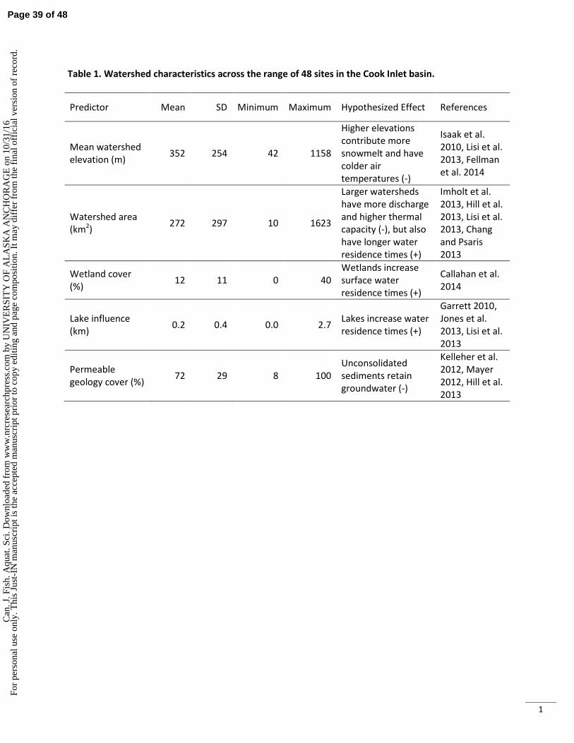
1
Table 1. Watershed characteristics across the range of 48 sites in the Cook Inlet basin.
Predictor Mean SD Minimum Maximum Hypothesized Effect References
Mean watershed
elevation (m) 352 254 42 1158
Higher elevations
contribute more
snowmelt and have
colder air
temperatures (-)
Isaak et al.
2010, Lisi et al.
2013, Fellman
et al. 2014
Watershed area
(km2)
272 297 10 1623
Larger watersheds
have more discharge
and higher thermal
capacity (-), but also
have longer water
residence times (+)
Imholt et al.
2013, Hill et al.
2013, Lisi et al.
2013, Chang
and Psaris
2013
Wetland cover
(%) 12 11 0 40
Wetlands increase
surface water
residence times (+)
Callahan et al.
2014
Lake influence
(km) 0.2 0.4 0.0 2.7
Lakes increase water
residence times (+)
Garrett 2010,
Jones et al.
2013, Lisi et al.
2013
Permeable
geology cover (%) 72 29 8 100
Unconsolidated
sediments retain
groundwater (-)
Kelleher et al.
2012, Mayer
2012, Hill et al.
2013
Page 39 of 48C
an. J
. Fis
h. A
quat
. Sci
. Dow
nloa
ded
from
ww
w.n
rcre
sear
chpr
ess.
com
by
UN
IVE
RSI
TY
OF
AL
ASK
A A
NC
HO
RA
GE
on
10/3
1/16
For
pers
onal
use
onl
y. T
his
Just
-IN
man
uscr
ipt i
s th
e ac
cept
ed m
anus
crip
t pri
or to
cop
y ed
iting
and
pag
e co
mpo
sitio
n. I
t may
dif
fer
from
the
fina
l off
icia
l ver
sion
of
reco
rd.
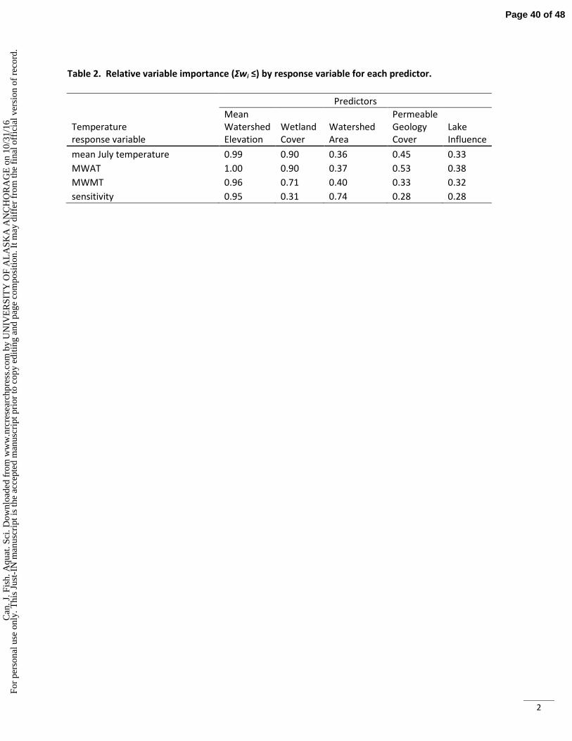
2
Table 2. Relative variable importance (Ʃwi ≤) by response variable for each predictor.
Predictors
Temperature
response variable
Mean
Watershed
Elevation
Wetland
Cover
Watershed
Area
Permeable
Geology
Cover
Lake
Influence
mean July temperature 0.99 0.90 0.36 0.45 0.33
MWAT 1.00 0.90 0.37 0.53 0.38
MWMT 0.96 0.71 0.40 0.33 0.32
sensitivity 0.95 0.31 0.74 0.28 0.28
Page 40 of 48C
an. J
. Fis
h. A
quat
. Sci
. Dow
nloa
ded
from
ww
w.n
rcre
sear
chpr
ess.
com
by
UN
IVE
RSI
TY
OF
AL
ASK
A A
NC
HO
RA
GE
on
10/3
1/16
For
pers
onal
use
onl
y. T
his
Just
-IN
man
uscr
ipt i
s th
e ac
cept
ed m
anus
crip
t pri
or to
cop
y ed
iting
and
pag
e co
mpo
sitio
n. I
t may
dif
fer
from
the
fina
l off
icia
l ver
sion
of
reco
rd.
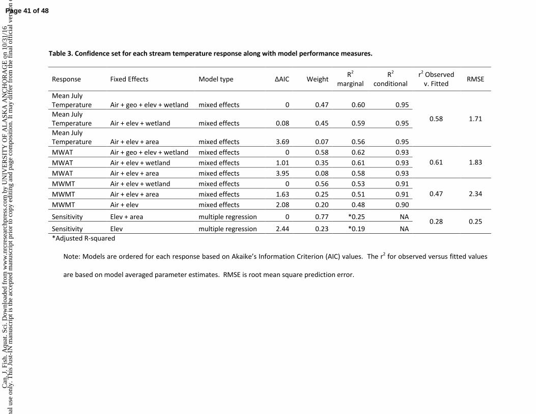
Table 3. Confidence set for each stream temperature response along with model performance measures.
Response Fixed Effects Model type ∆AIC Weight R
2
marginal
R2
conditional
r2 Observed
v. Fitted RMSE
Mean July
Temperature Air + geo + elev + wetland mixed effects 0 0.47 0.60 0.95
0.58 1.71 Mean July
Temperature Air + elev + wetland mixed effects 0.08 0.45 0.59 0.95
Mean July
Temperature Air + elev + area mixed effects 3.69 0.07 0.56 0.95
MWAT Air + geo + elev + wetland mixed effects 0 0.58 0.62 0.93
0.61 1.83 MWAT Air + elev + wetland mixed effects 1.01 0.35 0.61 0.93
MWAT Air + elev + area mixed effects 3.95 0.08 0.58 0.93
MWMT Air + elev + wetland mixed effects 0 0.56 0.53 0.91
0.47 2.34 MWMT Air + elev + area mixed effects 1.63 0.25 0.51 0.91
MWMT Air + elev mixed effects 2.08 0.20 0.48 0.90
Sensitivity Elev + area multiple regression 0 0.77 *0.25 NA 0.28 0.25
Sensitivity Elev multiple regression 2.44 0.23 *0.19 NA
*Adjusted R-squared
Note: Models are ordered for each response based on Akaike’s Information Criterion (AIC) values. The r2 for observed versus fitted values
are based on model averaged parameter estimates. RMSE is root mean square prediction error.
Page 41 of 48C
an. J
. Fis
h. A
quat
. Sci
. Dow
nloa
ded
from
ww
w.n
rcre
sear
chpr
ess.
com
by
UN
IVE
RSI
TY
OF
AL
ASK
A A
NC
HO
RA
GE
on
10/3
1/16
For
pers
onal
use
onl
y. T
his
Just
-IN
man
uscr
ipt i
s th
e ac
cept
ed m
anus
crip
t pri
or to
cop
y ed
iting
and
pag
e co
mpo
sitio
n. I
t may
dif
fer
from
the
fina
l off
icia
l ver
sion
of
reco
rd.
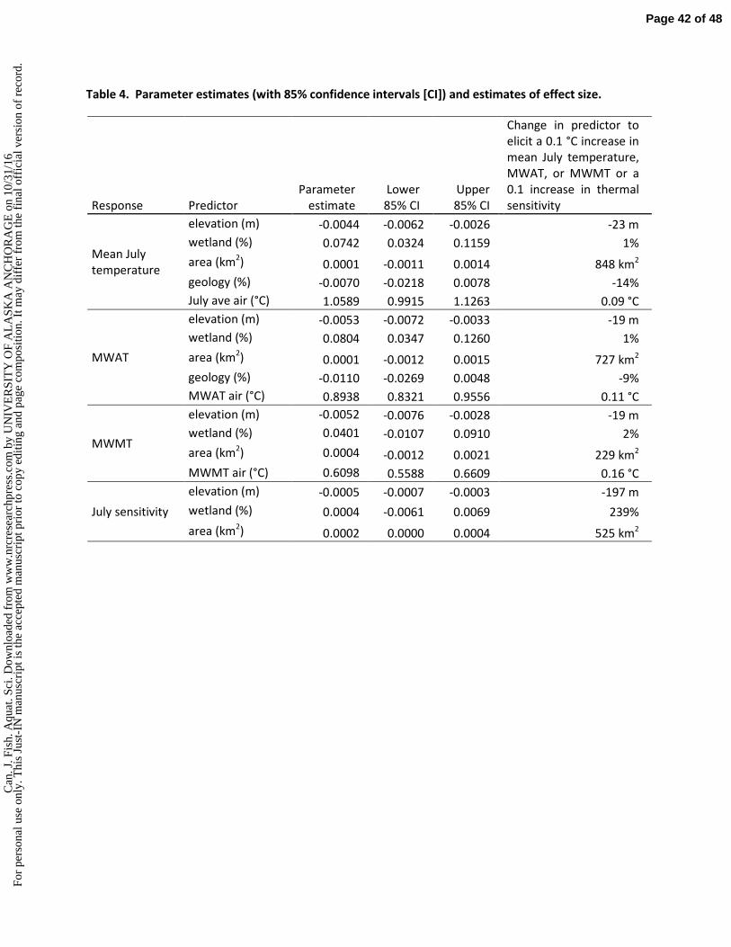
Table 4. Parameter estimates (with 85% confidence intervals [CI]) and estimates of effect size.
Response Predictor
Parameter
estimate
Lower
85% CI
Upper
85% CI
Change in predictor to
elicit a 0.1 °C increase in
mean July temperature,
MWAT, or MWMT or a
0.1 increase in thermal
sensitivity
Mean July
temperature
elevation (m) -0.0044 -0.0062 -0.0026 -23 m
wetland (%) 0.0742 0.0324 0.1159 1%
area (km2) 0.0001 -0.0011 0.0014 848 km
2
geology (%) -0.0070 -0.0218 0.0078 -14%
July ave air (°C) 1.0589 0.9915 1.1263 0.09 °C
MWAT
elevation (m) -0.0053 -0.0072 -0.0033 -19 m
wetland (%) 0.0804 0.0347 0.1260 1%
area (km2) 0.0001 -0.0012 0.0015 727 km
2
geology (%) -0.0110 -0.0269 0.0048 -9%
MWAT air (°C) 0.8938 0.8321 0.9556 0.11 °C
MWMT
elevation (m) -0.0052 -0.0076 -0.0028 -19 m
wetland (%) 0.0401 -0.0107 0.0910 2%
area (km2) 0.0004 -0.0012 0.0021 229 km
2
MWMT air (°C) 0.6098 0.5588 0.6609 0.16 °C
July sensitivity
elevation (m) -0.0005 -0.0007 -0.0003 -197 m
wetland (%) 0.0004 -0.0061 0.0069 239%
area (km2) 0.0002 0.0000 0.0004 525 km
2
Page 42 of 48C
an. J
. Fis
h. A
quat
. Sci
. Dow
nloa
ded
from
ww
w.n
rcre
sear
chpr
ess.
com
by
UN
IVE
RSI
TY
OF
AL
ASK
A A
NC
HO
RA
GE
on
10/3
1/16
For
pers
onal
use
onl
y. T
his
Just
-IN
man
uscr
ipt i
s th
e ac
cept
ed m
anus
crip
t pri
or to
cop
y ed
iting
and
pag
e co
mpo
sitio
n. I
t may
dif
fer
from
the
fina
l off
icia
l ver
sion
of
reco
rd.
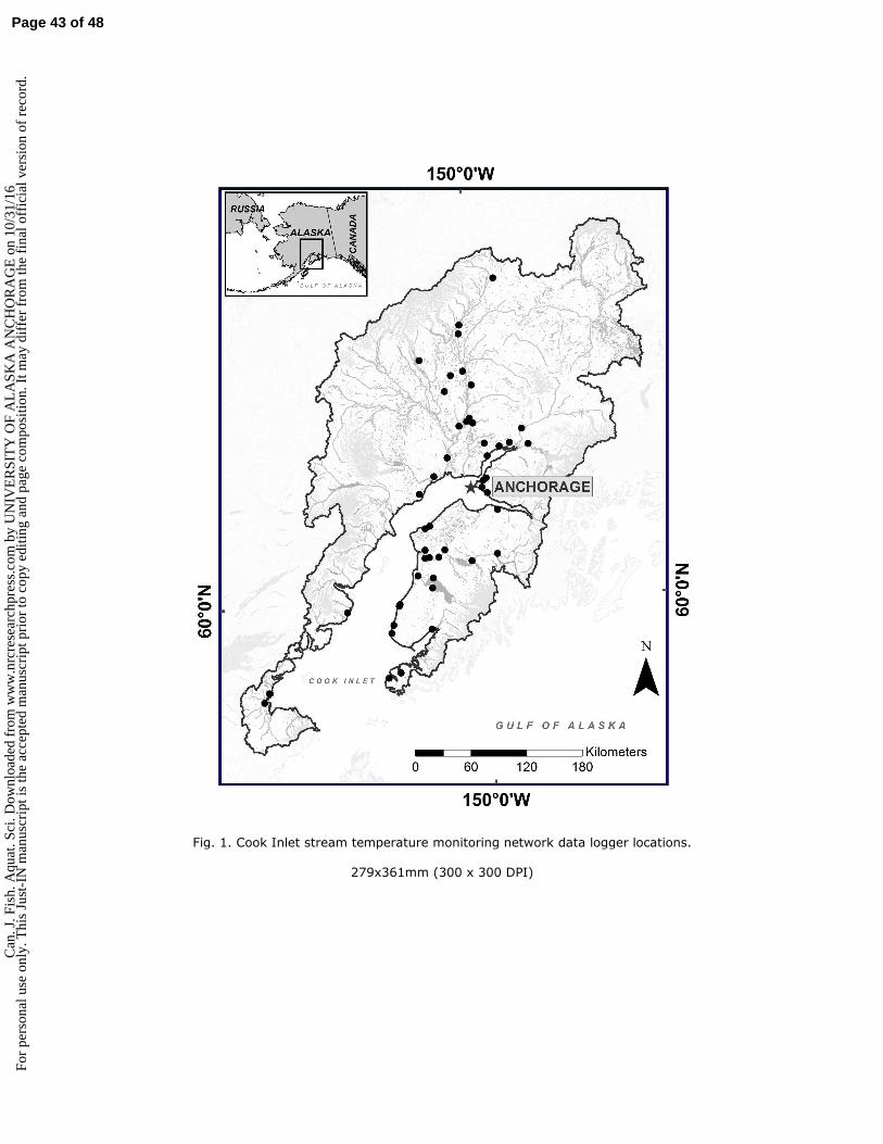
Fig. 1. Cook Inlet stream temperature monitoring network data logger locations.
279x361mm (300 x 300 DPI)
Page 43 of 48C
an. J
. Fis
h. A
quat
. Sci
. Dow
nloa
ded
from
ww
w.n
rcre
sear
chpr
ess.
com
by
UN
IVE
RSI
TY
OF
AL
ASK
A A
NC
HO
RA
GE
on
10/3
1/16
For
pers
onal
use
onl
y. T
his
Just
-IN
man
uscr
ipt i
s th
e ac
cept
ed m
anus
crip
t pri
or to
cop
y ed
iting
and
pag
e co
mpo
sitio
n. I
t may
dif
fer
from
the
fina
l off
icia
l ver
sion
of
reco
rd.
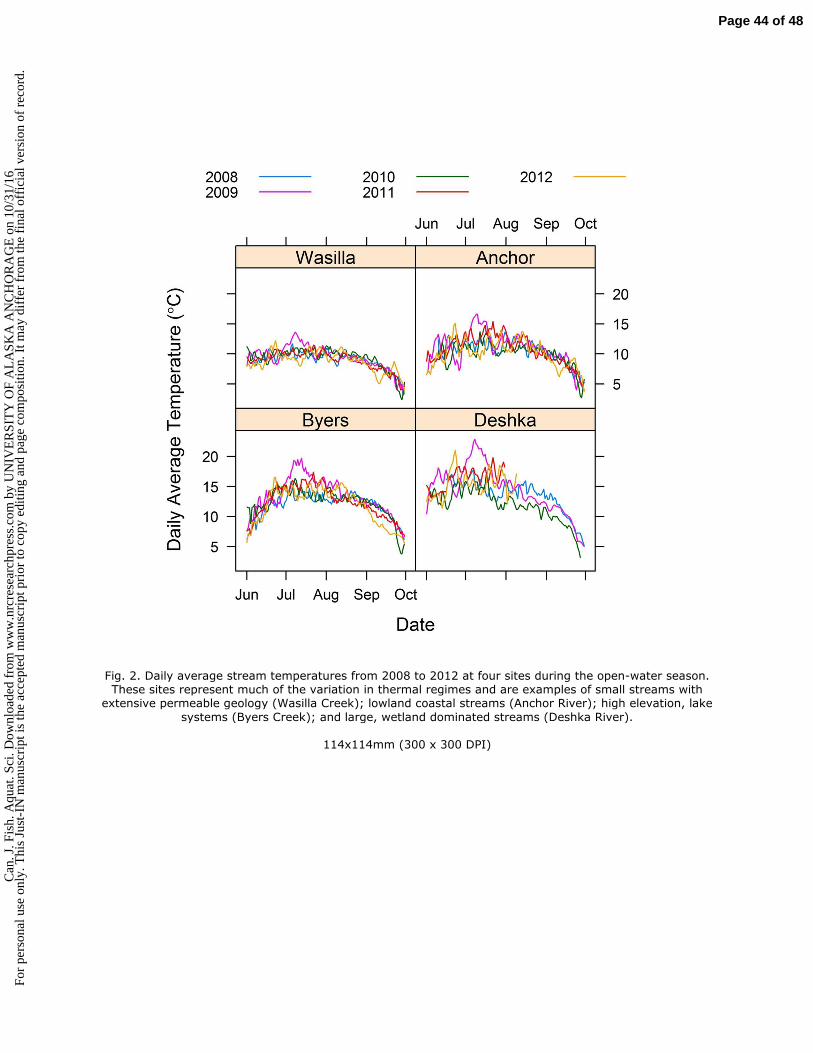
Fig. 2. Daily average stream temperatures from 2008 to 2012 at four sites during the open-water season. These sites represent much of the variation in thermal regimes and are examples of small streams with
extensive permeable geology (Wasilla Creek); lowland coastal streams (Anchor River); high elevation, lake
systems (Byers Creek); and large, wetland dominated streams (Deshka River).
114x114mm (300 x 300 DPI)
Page 44 of 48C
an. J
. Fis
h. A
quat
. Sci
. Dow
nloa
ded
from
ww
w.n
rcre
sear
chpr
ess.
com
by
UN
IVE
RSI
TY
OF
AL
ASK
A A
NC
HO
RA
GE
on
10/3
1/16
For
pers
onal
use
onl
y. T
his
Just
-IN
man
uscr
ipt i
s th
e ac
cept
ed m
anus
crip
t pri
or to
cop
y ed
iting
and
pag
e co
mpo
sitio
n. I
t may
dif
fer
from
the
fina
l off
icia
l ver
sion
of
reco
rd.
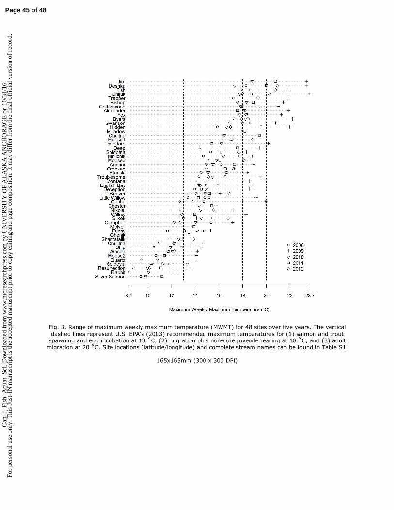
Fig. 3. Range of maximum weekly maximum temperature (MWMT) for 48 sites over five years. The vertical dashed lines represent U.S. EPA's (2003) recommended maximum temperatures for (1) salmon and trout spawning and egg incubation at 13 ˚C, (2) migration plus non-core juvenile rearing at 18 ˚C, and (3) adult migration at 20 ˚C. Site locations (latitude/longitude) and complete stream names can be found in Table S1.
165x165mm (300 x 300 DPI)
Page 45 of 48C
an. J
. Fis
h. A
quat
. Sci
. Dow
nloa
ded
from
ww
w.n
rcre
sear
chpr
ess.
com
by
UN
IVE
RSI
TY
OF
AL
ASK
A A
NC
HO
RA
GE
on
10/3
1/16
For
pers
onal
use
onl
y. T
his
Just
-IN
man
uscr
ipt i
s th
e ac
cept
ed m
anus
crip
t pri
or to
cop
y ed
iting
and
pag
e co
mpo
sitio
n. I
t may
dif
fer
from
the
fina
l off
icia
l ver
sion
of
reco
rd.
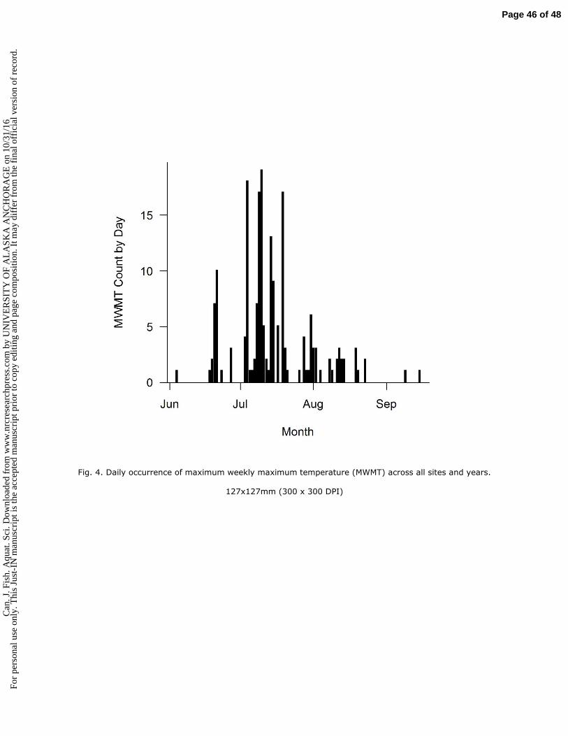
Fig. 4. Daily occurrence of maximum weekly maximum temperature (MWMT) across all sites and years.
127x127mm (300 x 300 DPI)
Page 46 of 48C
an. J
. Fis
h. A
quat
. Sci
. Dow
nloa
ded
from
ww
w.n
rcre
sear
chpr
ess.
com
by
UN
IVE
RSI
TY
OF
AL
ASK
A A
NC
HO
RA
GE
on
10/3
1/16
For
pers
onal
use
onl
y. T
his
Just
-IN
man
uscr
ipt i
s th
e ac
cept
ed m
anus
crip
t pri
or to
cop
y ed
iting
and
pag
e co
mpo
sitio
n. I
t may
dif
fer
from
the
fina
l off
icia
l ver
sion
of
reco
rd.
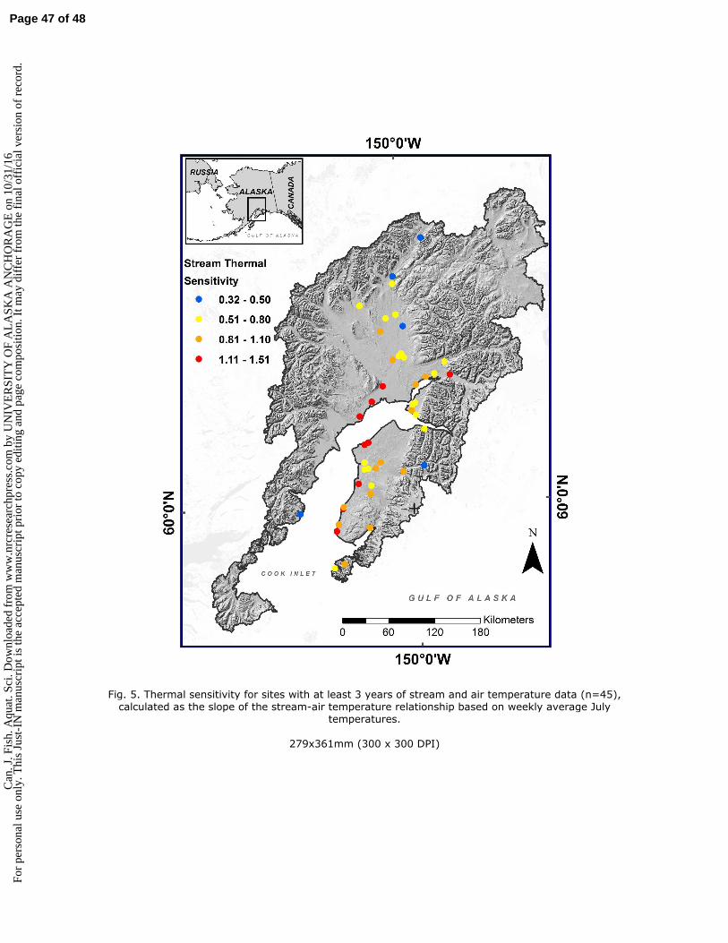
Fig. 5. Thermal sensitivity for sites with at least 3 years of stream and air temperature data (n=45), calculated as the slope of the stream-air temperature relationship based on weekly average July
temperatures.
279x361mm (300 x 300 DPI)
Page 47 of 48C
an. J
. Fis
h. A
quat
. Sci
. Dow
nloa
ded
from
ww
w.n
rcre
sear
chpr
ess.
com
by
UN
IVE
RSI
TY
OF
AL
ASK
A A
NC
HO
RA
GE
on
10/3
1/16
For
pers
onal
use
onl
y. T
his
Just
-IN
man
uscr
ipt i
s th
e ac
cept
ed m
anus
crip
t pri
or to
cop
y ed
iting
and
pag
e co
mpo
sitio
n. I
t may
dif
fer
from
the
fina
l off
icia
l ver
sion
of
reco
rd.
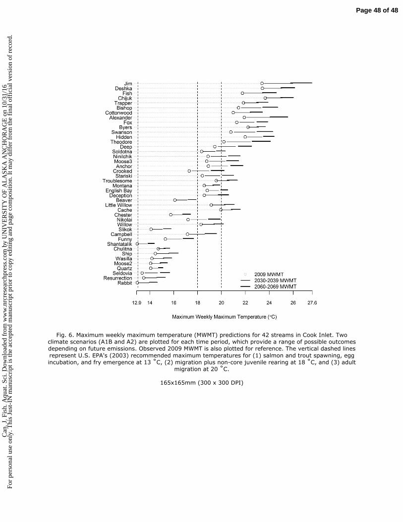
Fig. 6. Maximum weekly maximum temperature (MWMT) predictions for 42 streams in Cook Inlet. Two climate scenarios (A1B and A2) are plotted for each time period, which provide a range of possible outcomes depending on future emissions. Observed 2009 MWMT is also plotted for reference. The vertical dashed lines represent U.S. EPA's (2003) recommended maximum temperatures for (1) salmon and trout spawning, egg incubation, and fry emergence at 13 ˚C, (2) migration plus non-core juvenile rearing at 18 ˚C, and (3) adult
migration at 20 ˚C.
165x165mm (300 x 300 DPI)
Page 48 of 48C
an. J
. Fis
h. A
quat
. Sci
. Dow
nloa
ded
from
ww
w.n
rcre
sear
chpr
ess.
com
by
UN
IVE
RSI
TY
OF
AL
ASK
A A
NC
HO
RA
GE
on
10/3
1/16
For
pers
onal
use
onl
y. T
his
Just
-IN
man
uscr
ipt i
s th
e ac
cept
ed m
anus
crip
t pri
or to
cop
y ed
iting
and
pag
e co
mpo
sitio
n. I
t may
dif
fer
from
the
fina
l off
icia
l ver
sion
of
reco
rd.