P & I Design Ltd - CHEMCAD is a suite of chemical process ... · 1 Ideal Solution Txy Diagram ... R.C. Reid, J.M. Prausnitz, B.E. Poling,“The Properties of Gases ... based on a

P & I Design Ltd Process Instrumentation Consultancy & Design

2 Reed Street, Gladstone Industrial Estate, Thornaby, TS17 7AF, United Kingdom.

Tel. +44 (0) 1642 617444 Fax. +44 (0) 1642 616447 Web Site: www.pidesign.co.uk

PROCESS MODELLING

SELECTION OF

THERMODYNAMIC METHODS

by John E. Edwards

[email protected]

MNL031B 10/08 PAGE 1 OF 38

mailto:[email protected]�

Process Modelling Selection of Thermodynamic Methods

PAGE 2 OF 38

MNL 031B Issued November 2008, Prepared by J.E.Edwards of P & I Design Ltd, Teesside, UK www.pidesign.co.uk

3.2 Liquid Phase

Contents 1.0 Introduction 2.0 Thermodynamic Fundamentals 2.1 Thermodynamic Energies 2.2 Gibbs Phase Rule 2.3 Enthalpy 2.4 Thermodynamics of Real Processes 3.0 System Phases 3.1 Single Phase Gas

3.3 Vapour liquid equilibrium 4.0 Chemical Reactions 4.1 Reaction Chemistry 4.2 Reaction Chemistry Applied 5.0 Summary

Appendices

I Enthalpy Calculations in CHEMCAD II Thermodynamic Model Synopsis – Vapor Liquid Equilibrium III Thermodynamic Model Selection – Application Tables IV K Model – Henry’s Law Review V Inert Gases and Infinitely Dilute Solutions VI Post Combustion Carbon Capture Thermodynamics VII Thermodynamic Guidance Note VIII Prediction of Physical Properties

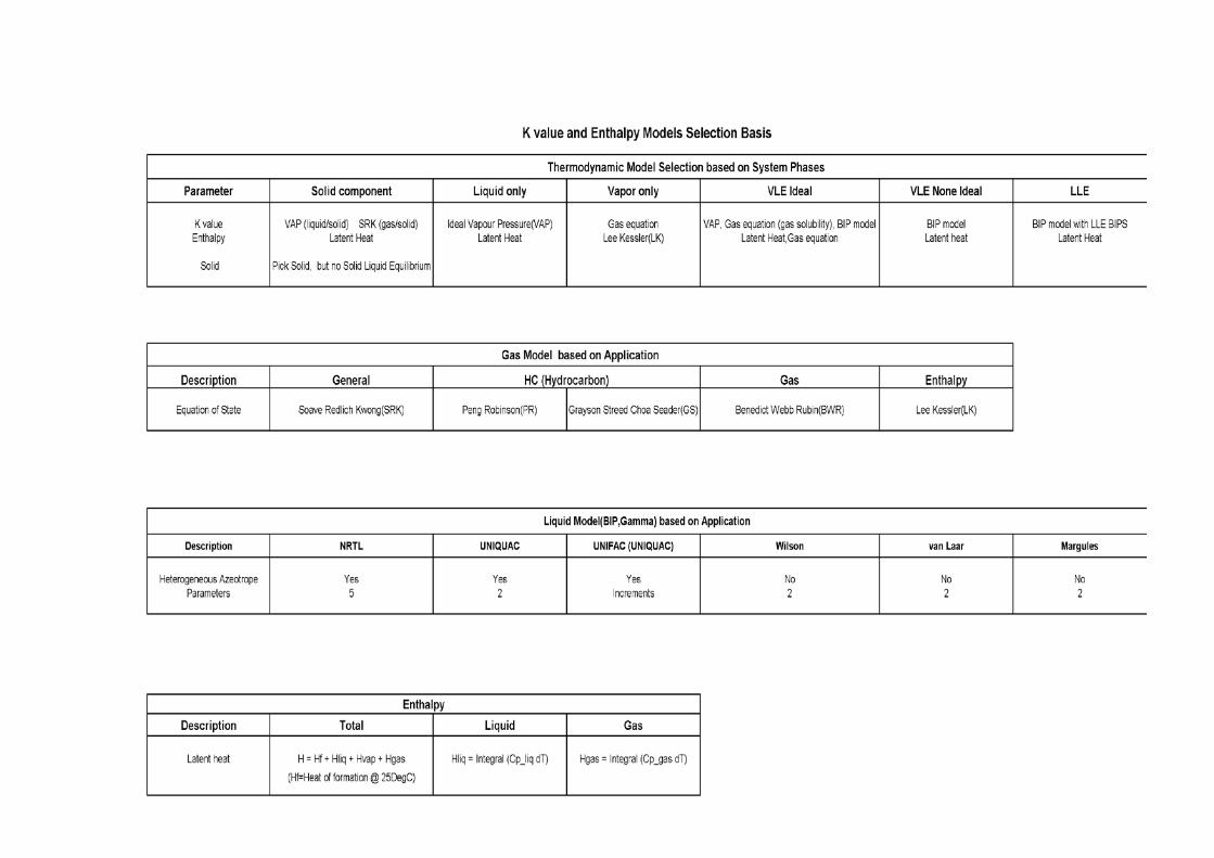
Figures 1 Ideal Solution Txy Diagram 2 Enthalpy Isobar 3 Thermodynamic Phases 4 van der Waals Equation of State 5 Relative Volatility in VLE Diagram 6 Azeotrope γ Value in VLE Diagram 7 VLE Diagram and Convergence Effects 8 CHEMCAD K and H Values Wizard 9 Thermodynamic Model Decision Tree 10 K Value and Enthalpy Models Selection Basis

http://www.pidesign.co.uk/�


PAGE 3 OF 38


References

1. C.C. Coffin, J.Chem.Education 23, 584-588 (1946), “A Presentation of the Thermodynamic Functions”.

2. R.M. Felder and R.W. Rousseau, “Elementary Principles of Chemical Processes”, 2nd Edition, John Wiley and Sons.

3. R.C. Reid, J.M. Prausnitz, B.E. Poling, “The Properties of Gases and Liquids”, 4th Edition, McGraw Hill.

4. I. Smallwood, “Solvent Recovery Handbook”, Edward Arnold, 1993. 5. R.H.Perry, “Chemical Engineers’ Handbook”, McGraw Hill. 6. R.Sander, “Compilation of Henry’s Law Constants for Inorganic and Organic Species of

Potential Importance in Environmental Chemistry”, Max-Planck Institute, Version 3, April 1999.

7. J.R.W.Warn, “Concise Chemical Thermodynamics”, van Rostrand Reinhold, 1969. 8. Kent, R. L. and Eisenberg, Hydrocarbon Processing, Feb. 1976, p. 87-92. 9. F.G. Shinskey, “Process Control Systems”, McGraw-Hill, 1967. 10. O.Levenspiel, “Chemical Reaction Engineering”, Wiley, 2nd Edition, 1972. 11. J.Wilday and J.Etchells, “Workbook for Chemical Reactor Relief Sizing”, HSE Contract

Research Report 136/1998. 12. H.S.Fogler, “Elements of Chemical Reaction Engineering”, 3rd Edition, Prentice Hall, p122. 13. K.J.Laidler, “Theories of Chemical Reaction Rates”, New York, R.E.Krieger, 1979, p38.

Acknowledgements

This paper has been developed from experience gained whilst working in the simulation field. This work has been supported throughout by Chemstations, Houston, Texas, TX77042 www.chemstations.com and the author is particularly indebted to Aaron Herrick and David Hill for their continued and unstinting help.


http://www.chemstations.com/�


PAGE 4 OF 38


1.0 INTRODUCTION

The selection of a suitable thermodynamic model for the prediction of the enthalpy-H and the phase equilibrium-K is fundamental to process modelling. An inappropriate model selection will result in convergence problems and erroneous results. Simulations are only valid when the appropriate thermodynamic model is being used. The selection process is based on a detailed knowledge of thermodynamics and practical experience. Most simulators are provided with Wizards to aid selection which should be used with caution. The selection process is guided by considering the following:-

Process species and compositions. Pressure and temperature operating ranges. System phases involved. Nature of the fluids. Availability of data.

There are four categories of thermodynamic models:-

Equations-of-State (E-o-S) Activity coefficient (γ) Empirical Special system specific

This paper is not intended to be a rigorous analysis of the methods available or in their selection but is offered as an “aide memoire” to the practicing engineer who is looking for rapid, realistic results from his process models. The study of complex systems invariably involves extensive research and considerable investment in manpower effort by specialists. There are extensive sources of physical property data available from organisations such as DECHEMA www.dechema.de, DIPPR www.aiche.org/dippr/ , TÜV NEL Ltd www.ppds.co.uk amongst others. This paper presents selection methods developed in discussions with engineers in the field. The validity of the thermodynamic models being used should be tested against known data whenever possible.


http://www.dechema.de/�

http://www.aiche.org/dippr/�

http://www.ppds.co.uk/�


PAGE 5 OF 38


2.0 THERMODYNAMIC FUNDAMENTALS 2.1 Thermodynamic Energies(1)

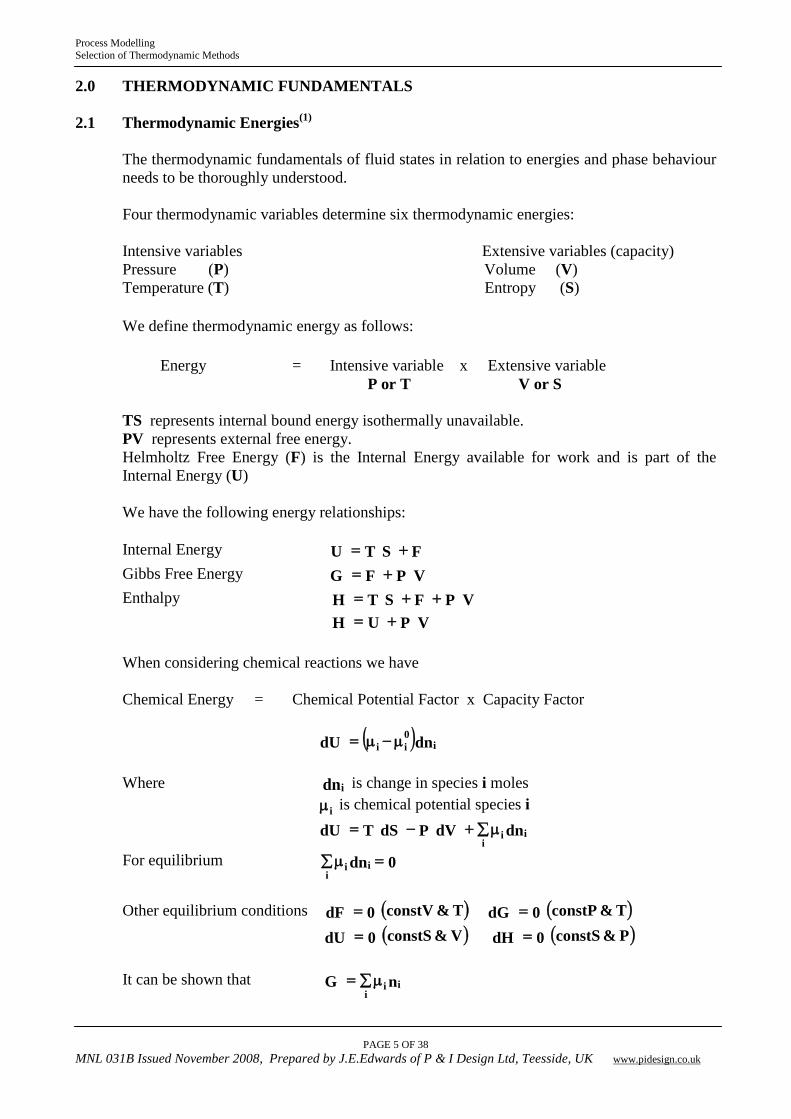
The thermodynamic fundamentals of fluid states in relation to energies and phase behaviour needs to be thoroughly understood. Four thermodynamic variables determine six thermodynamic energies: Intensive variables Extensive variables (capacity) Pressure (P) Volume (V) Temperature (T) Entropy (S) We define thermodynamic energy as follows: Energy = Intensive variable x Extensive variable P or T V or S TS represents internal bound energy isothermally unavailable. PV represents external free energy. Helmholtz Free Energy (F) is the Internal Energy available for work and is part of the Internal Energy (U) We have the following energy relationships: Internal Energy FSTU += Gibbs Free Energy VPFG += Enthalpy VPFSTH ++= VPUH += When considering chemical reactions we have Chemical Energy = Chemical Potential Factor x Capacity Factor ( )dndU i

0ii µ−µ=

Where dni is change in species i moles

µi is chemical potential species i dndVPdSTdU i

ii∑µ+−=

For equilibrium 0dnii

i =∑µ

Other equilibrium conditions ( )T&constV0dF = ( )T&constP0dG = ( )V&constS0dU = ( )P&constS0dH = It can be shown that nG i

ii∑µ=



PAGE 6 OF 38


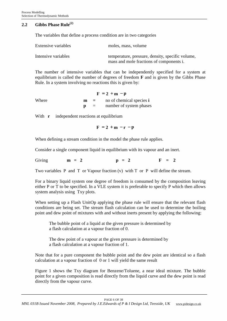
2.2 Gibbs Phase Rule(2)

The variables that define a process condition are in two categories Extensive variables moles, mass, volume Intensive variables temperature, pressure, density, specific volume, mass and mole fractions of components i. The number of intensive variables that can be independently specified for a system at equilibrium is called the number of degrees of freedom F and is given by the Gibbs Phase Rule. In a system involving no reactions this is given by: pm2F −+= Where m = no of chemical species i p = number of system phases With r independent reactions at equilibrium prm2F −−+= When defining a stream condition in the model the phase rule applies. Consider a single component liquid in equilibrium with its vapour and an inert. Giving m = 2 p = 2 F = 2 Two variables P and T or Vapour fraction (v) with T or P will define the stream. For a binary liquid system one degree of freedom is consumed by the composition leaving either P or T to be specified. In a VLE system it is preferable to specify P which then allows system analysis using Txy plots. When setting up a Flash UnitOp applying the phase rule will ensure that the relevant flash conditions are being set. The stream flash calculation can be used to determine the boiling point and dew point of mixtures with and without inerts present by applying the following:

The bubble point of a liquid at the given pressure is determined by a flash calculation at a vapour fraction of 0.

The dew point of a vapour at the given pressure is determined by a flash calculation at a vapour fraction of 1.

Note that for a pure component the bubble point and the dew point are identical so a flash calculation at a vapour fraction of 0 or 1 will yield the same result Figure 1 shows the Txy diagram for Benzene/Toluene, a near ideal mixture. The bubble point for a given composition is read directly from the liquid curve and the dew point is read directly from the vapour curve.



PAGE 7 OF 38


2.2 Gibbs Phase Rule(2)(Cont)

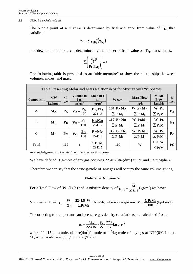
The bubble point of a mixture is determined by trial and error from value of Tbp that satisfies: The dewpoint of a mixture is determined by trial and error from value of Tdp that satisfies:

The following table is presented as an “aide memoire” to show the relationships between volumes, moles, and mass.

Table Presenting Molar and Mass Relationships for Mixture with “i” Species

Component MW % v/v

Volume in 1 m3

Mass in 1 m3 % w/w Mass Flow Molar

Flow % mol kg/kmol m3/m3 kg/m3 kg/h kmol/h

A MA PA 100PV A

A = 5.2241

MP AA ∑ MP

MP100

ii

AA ∑ MP

MPW

ii

AA ∑ MP

PW

ii

A PA

B MB PB 100PV B

B = 5.2241

MP BB ∑ MP

MP100

ii

BB ∑ MP

MPW

ii

BB ∑ MP

PW

ii

B PB

C MC PC 100PV C

C = 5.2241

MP CC ∑ MP

MP100

ii

CC ∑ MP

MPW

ii

CC ∑ MP

PW

ii

C PC

Total 100 1 5.2241

MP ii∑ 100 W ∑ MP

W100

ii 100

Acknowledgements to the late Doug Lindsley for this format. We have defined: 1 g-mole of any gas occupies 22.415 litre(dm3) at 0ºC and 1 atmosphere. Therefore we can say that the same g-mole of any gas will occupy the same volume giving:

Mole % = Volume %

For a Total Flow of W (kg/h) and a mixture density of 5.2241

M__

0G =ρ (kg/m3) we have:

Volumetric Flow ∑

==MP

W5.2241GW

QiiO

(Nm3/h) where average mw 100

MPM ii__ ∑= (kg/kmol)

To correcting for temperature and pressure gas density calculations are calculated from:

where 22.415 is in units of litre(dm3)/g-mole or m3/kg-mole of any gas at NTP(0ºC,1atm), Mw is molecular weight g/mol or kg/kmol.

( )TpxP bp*ii∑=

( ) 1TpPy

dp*i

i =

∑

m/kgT

273ZP

415.22M 3

ff

fWG ××=ρ



PAGE 8 OF 38


2.3 Enthalpy

Enthalpy is the sum of the internal energy (U) and the external free energy (PV) where: VPUH += The heat supplied is given by:

dVPdUdQ += The sign convention should be noted and is + for heat added and dU gain in internal energy dTCdU v= The specific heat at constant pressure Cp is related to heat input: dTCdQ p= The adiabatic index or specific ratio γ is defined:

CC

v

p=γ It can be shown that the following relationship holds

RCC vp =− The heating of a liquid at constant pressure e.g. water is considered in Figure 2. This shows the relationships between the enthalpies in the different phases namely the sensible heat in the liquid phase, the latent heat of vaporisation during the vapour liquid equilibrium phase and the superheat in the gas phase. Enthalpy is calculated using Latent Heat (LATE) in the liquid and vle phases and E-o-S (SRK) in the superheated or gas phase. Appendix I reviews the calculation methods adopted in CHEMCAD. A standard reference state of 298ºK for the liquid heat of formation is used providing the advantage that the pressure has no influence on the liquid Cp. The enthalpy method used will depend on the K-value method selected as detailed in Appendix II. CHEMCAD forces the following H-values from K-value selected.

Equilibrium-K Enthalpy-H Peng Robinson (PR) PR Grayson-Streed-Choa-Seeder(GS) Lee Kessler (LK) ESSO LK Benedict-Webb-Rubin-Starling (BWRS) BWRS AMINE AMINE

Special methods are used for: Enthalpy of water steam tables (empirical) Acid gas absorption by DEA and MEA Solid components



PAGE 9 OF 38


2.4 Thermodynamics of Real Processes(7)

To establish if a real process is possible we need to consider:

STHG ∆∆∆ −= The values for ∆H are determined from the heats of formation of the components and for ∆S from thermodynamic property tables. Superscript 0 indicates materials present in standard state at 298ºK. For isothermal processes at low temperature the ∆H term is dominant. At absolute zero ∆S and T are zero so ∆G = ∆H. The relationship shows ∆S becoming of increasing importance as the temperature increases. Adsorption Processes The enthalpy change is ∆H = ∆G + T∆S with ∆G being necessarily negative. All adsorptions with negative entropy change, which comprise all physical and the great majority of chemical adsorptions, are exothermic. Evaporation Processes When a liquid boils the vapour pressure is equal to the atmospheric pressure and the vapour is in equilibrium with the liquid. If there is no superheat the process is reversible and ∆G = 0 and the entropy change can be calculated:

TH

SB

onvaporisati∆∆ =

Entropies of vaporisation, at these conditions, have values near 88 J/molºK, and substitution in the above gives Trouton’s rule. However in the case of water, due to significant hydrogen bonding, the entropy change on evaporation is larger at 108.8 J/molºK. Endothermic Chemical Processes

The link between Gibbs free energy and the reaction equilibrium constant K is represented by the equation

∆G = -RT log K A reaction will proceed provided ∆G is negative. The reaction temperature can alter the sign and therefore the process feasibility. Chemical Equilibrium For a reaction at equilibrium (all reactions can be considered equilibrium since no reaction goes to completion) there is no net reaction in either direction and we have:

∆G = 0 In CHEMCAD the Gibbs reactor is based on the principal that at chemical equilibrium the total Gibbs free energy of the system is at its minimum value. The Gibbs reactor can be used in the study of combustion processes including adjustment of air to fuel ratios and calculation of the heats of reaction.



PAGE 10 OF 38


3.0 SYSTEM PHASES

There are three phase states namely solid, liquid and gas. Processes comprise either single phase or multiphase systems with separation processes involving at least two phases. Processes involving solids such as filtration and crystallisation, solid – liquid systems and drying, solid – gas system are special cases and receive no further consideration here. The primary area of interest for thermodynamic model selection involve two phases. Liquid – liquid systems, such as extraction and extractive distillation, where liquid – liquid equilibrium (LLE) is considered and vapour liquid systems, such as distillation, stripping and absorption, where vapour – liquid equilibrium (VLE) is considered. Figure 3 shows the inter-relationships between the system phases for a series of isotherms based on the Equation of State (E-o-S) due to van-der-Waal. This figure provides the first indication of the validity of making a thermodynamic model selection for the K-value on the basis of the system phases namely single phase gas by E-o-S and VLE by activity coefficient.

3.1 Single Phase Gas(2)

An E-o-S relates the quantity and volume of gas to the temperature and pressure. The ideal gas law is the simplest E-o-S

TRnVP =

Where P = absolute pressure of gas V = volume or volume of rate of flow n = number of moles or molar flowrate R = gas constant in consistent units T = absolute temperature In an ideal gas mixture the individual components and the mixture as a whole behave in an ideal manner which yields for component i the following relationships TRnVP ii =

ynn

Pp

iii == where yi is mole fraction of i in gas

Pyp ii = Pp

ii =∑ where P is the total system pressure

plnTR i0ii +µ=µ

Note that when pi = 1 we have µ=µ 0ii the reference condition

As the system temperature decreases and the pressure increases deviations from the ideal gas E-o-S result. There are many equation of state(3) available for predicting non-ideal gas behaviour and another method incorporates a compressibility factor into the ideal gas law.



PAGE 11 OF 38


3.1 Single Phase Gas(2) (Cont) To predict the behaviour of real gases the concept of fugacity f is introduced giving: flnTR i

0ii +µ=µ

Fugacity and pressure become identical at zero pressure, where limitP→0

→ 1

Pf

Fugacity is not the actual pressure. It has to account for the actual behaviour of real gases and to overcome the assumption of perfect behaviour being still part of the basic equation.

Fugacity is of importance when considering processes exhibiting highly non-ideal behaviour

involving vapour liquid equilibrium. Virial Equation of State is given by the following:

( ) ( )

+++=V

TCV

TB1

TRVP

2

Where B(T) is the second virial coefficient C(T) is the third virial coefficient Note if B = C = 0 the equation reduces to the ideal gas law. Benedict–Webb–Rubin (BWR) Equation of State This E-o-S is in the same form as the above equation extended to a fifth virial coefficient. BWR is accurate for gases containing a single species or a gas mixture with a dominant component e.g. natural gas, and provides considerable precision. Cubic Equations of State This represents an E-o-S linear in pressure and cubic in volume and is equivalent to the virial equation truncated at the third virial coefficient. One of the first E-o-S was that due to van der Waals (University of Leiden), developed in 1873, which is shown in Figure 4. This was based on two effects 1. The volume of the molecules reduces the amount of free volume in the fluid, (V-b) 2. Molecular attraction produces additional pressure. The fluid pressure is corrected by a term related to the attraction parameter a of the molecules, (P+a/V2) The resulting equation is:

( ) Va

bVTR

P 2−−

=

From the relationship: ( )dp

flndTRV = it can be shown for van der Waals equation:

( ) ( ) VTRa2

bVb

bVTR

lnfln −−

+−

=



PAGE 12 OF 38


3.1 Single Phase Gas(2) (Cont) The most widely used cubic E-o-S is the Soave modifications of the Redlich-Kwong (SRK) equation which is a modification to van der Waals original equation.

( ) ( )bVVa

bVTR

P+

α−

−=

Where α, a and b are system parameters. Parameters a and b are determined from the critical temperature Tc and critical Pressure Pc. Parameter α is determined from a correlation based on experimental data which uses a constant called the Pitzer Accentric Factor(3). At the critical point the two phases (gas and liquid) have exactly the same density (technically one phase). If T > Tc no phase change occurs. Refer to Figure 2. Appendix VIII reviews the prediction of physical properties in further detail.

Compressibility Factor Equation of State The Compressibility Factor E-o-S retains the simplicity of the ideal gas law but is applicable over a much wider range of conditions. TRnzVP = where z is the compressibility factor. The compressibility factor, dependent on the gas temperature and pressure, varies for different gases and is determined from reference data(5). If data is not available for the specific gas generalised compressibility charts can be used which require the critical temperature and critical pressure of the gas For single phase gas systems the following guidelines for thermodynamic model selection are proposed:

Process Application Equilibrium-K Enthalpy-H Hydrocarbon systems Pressure > 1 bar Soave-Redlich-Kwong (SRK) SRK or LATE

Non-polar hydrocarbons Pressure < 200 bar Temperature -18ºC to 430ºC

Grayson-Streed-Choa-Seeder(GS) Lee Kessler (LK)

Hydrocarbon systems Pressure > 10 bar Good for cryogenic systems

Peng Robinson (PR) PR

Single species gas system Gas compression Benedict-Webb-Rubin-Starling (BWRS) BWRS



PAGE 13 OF 38


3.2 Liquid Phase

On systems involving liquid phases the thermodynamic K-value selection is driven by the nature of the solution. Appendix II provides a summary of thermodynamic selection criteria considered in this section. The following five categories are considered: Ideal solution These solutions are non-polar and typically involve hydrocarbons in the same homologous series. Non-ideal solution – regular These solutions exhibit mildly non ideal behaviour and are usually non-polar in nature. Polar solutions – non-electrolyte These exhibit highly non-ideal behaviour and will use activity coefficient or special K-value models. Polar solutions – electrolyte Electrolytes are not considered in detail here. However, it should be noted that in modelling they can be treated as true species (molecules and ions) or apparent species (molecules only) There are two methods

MNRTL uses K-value NRTL and H LATE

Pitzer method has no restrictions Binary interaction parameters (BIPs) are required by both methods for accurate modelling. Special Special models have been developed for specific systems. In non-polar applications, such as hydrocarbon processing and refining, due to the complex nature of the mixtures and the large number of species pseudo components are created based on average boiling point, specific gravity and molecular weight. The alternative is to specify all species by molecular formula i.e. real components.



PAGE 14 OF 38


3.2 Liquid Phase (Cont.) Ideal Solutions(3)

In an ideal solution the chemical potential μi for species i is of the form: ( )xlnTR i

0ii +µ=µ

where µ0

i is the chemical potential of pure component i If an ideal solution is considered in equilibrium with a perfect gas the phase rule demonstrates that the two phases at a given T and P are not independent. Raoult’s Law describes the distribution of species i between the gas and the liquid phases pxPyp 0

iiii == at temperature T Raoult’s Law is valid when xi is close to 1 as in the case of a single component liquid and over the entire composition range for mixtures with components of similar molecular structure, size and chemical nature. The members of homologous series tend to form ideal mixtures in which the activity coefficient γ is close to 1 throughout the concentration range. The following systems can be considered suitable for Raoult’s Law. 1 Aliphatic hydrocarbons

Paraffins CnH2n+2 n-hexane (C6H14) n-heptane (C7H16) Olefines CnH2n Alcohols CnH2n+1•OH methanol (CH3•OH) ethanol (C2H5•OH)

2 Aromatic hydrocarbons benzene (C6H6) toluene (C6H5•CH3)

For ideal liquid systems the following guidelines for thermodynamic model selection are proposed

Equilibrium-K Enthalpy-H Ideal Vapour Pressure(VAP) SRK

In dilute solutions when xi is close to 0 and with no dissociation, ionisation or reaction in the liquid phase Henry’s law applies where: HxPyp iiii == at temperature T Henry’s law constants Hi for species i in given solvents are available. Typical applications include slightly soluble gases in aqueous systems. Refer Appendix IV for further details.



PAGE 15 OF 38


3.2 Liquid Phase (Cont.) Non-ideal solutions(3)

In a non ideal solution the chemical potential μi for species i is of the form:- ( )xlnTR i i

0ii γ+µ=µ

Where γi is the activity coefficient and component activity xa iii γ= Consider a non-ideal solution in equilibrium with a perfect gas we can derive an equation of the form: xkp iiii γ=

Raoult’s law when γi→1 and xi→1 pk 0ii = giving 1

xpp

i0i

ii ==γ

Henry’s law when γi→1 and xi→ 0 giving Hk ii = For vapour liquid equilibrium at temperature T and pressure P the condition of thermodynamic equilibrium for every component i in a mixture is given by: ff livi =

Where the fugacity coefficient Py

fi

vii=φ note 1i =φ for ideal gases

The fugacity of component i in the liquid phase is related to the composition of that phase by the activity coefficient γ as follows:

fx

fxa

0ii

li

i

ii ==γ

The standard state fugacity f 0i is at some arbitrarily chosen P and T and in non-electrolyte

systems is the fugacity of the pure component at system T and P. Regular solutions Regular solutions exhibit mildly non-ideal behaviour and occur in non-polar systems where the component molecular size, structure and chemical nature do not differ greatly. These systems can be modelled using an E-o-S.

K-values are calculated from the following relationships using fugacity coefficients

φφ

==vi

li

i

ii

xy

K where fugacity coefficients Pf vi

vi =φ and Px

fi

lili =φ

Process Application Equilibrium-K Enthalpy-H General hydrocarbon (same homologous series) System pressure > 10 bar PR PR

Branch chained hydrocarbon System pressure > 1 bar SRK SRK

Heavy end hydrocarbons System pressure < 7 bar Temperature 90C to430C ESSO LK

Branch-chained and halogenated hydrocarbon Some polar compounds MSRK SRK



PAGE 16 OF 38


3.2 Liquid Phase (Cont.) Polar non-electrolyte solutions These are systems where the liquid phase non-idealities arise predominantly from molecular associations. These systems must be modelled using activity coefficient methods which will require binary interaction parameters for accuracy. The vapor phase is taken to be a regular solution giving

Pf

xy

Kvi

0lii

vi

li

i

ii φ

γ=

φφ

==

Where f0li standard fugacity comp i

φvi fugacity coefficient vapour comp i γi activity coefficient

Models covered by the activity coefficient method include NRTL, UNIQUAC, Wilson, UNIFAC, HRNM, Van Laar, Margules and GMAC.

In making a selection the following should be considered

Wilson, NRTL, and UNIQUAC When sufficient data is available (>50%) UNIFAC When data is incomplete (<50%)



PAGE 17 OF 38


3.3 Vapour Liquid Equilibrium(4)

VLE diagrams provide a very useful source of information in relation to the suitability of the K-value selected and the problems presented for the proposed separation. Having selected a K-value method test the TPxy and VLE diagrams against known data for the pure components and azeotropes if present. Figure 5 in the attachments shows the VLE diagrams for N-Hexane systems. N-Hexane(1)/N-Heptane(2) can be considered close to representing ideal behaviour which is indicated by the curve symmetry (γ ≅ 1).The different binary systems presented in Figure 5 demonstrate the effect of an increasing α and its influence on ease of separation. We can investigate the effect of γ on α by considering the following

pxp 0

1111 γ= and pxp 02222 γ=

γγ

α=γ

γ=α

2

10022

011

pp

where α0 is the ideal mixture value

Since γ > 1 is the usual situation, except in molecules of a very different size, the actual relative volatility is very often much less than the ideal relative volatility particularly at the column top. Values of γ can be calculated throughout the concentration range using van Laar’s equation

+=γ

xAxA1

1Aln

221112

2

121 where γ= ∞112 lnA with ∞ representing infinite dilution

An extensive data bank providing values of parameter Axy are available from DECHEMA. Values of γ can also be calculated at an azeotrope which can be very useful due to the extensive azeotropic data available in the literature.

At an azeotrope we have yx 11 = giving pxPy 01111 γ= resulting in

pP

01

1 =γ

Figure 6 in the attachments shows the VLE diagrams for N-Hexane(1)/Ethyl Acetate(2) system. CHEMCAD Wizard selected K-value NRTL and H Latent Heat and it can be seen that the model is reasonably accurate against known data. The γ values are shown and their influence seen at the column bottom and top. Figure 7 in the attachments shows the VLE diagrams for Ethanol(1)/Water(2) using K-value method NRTL and SRK which clearly demonstrates the importance of model selection. To achieve convergence for high purity near the azeotropic composition it is recommended to start the simulation with “slack” parameters which can be loaded as initial column profile (set flag) and then tighten the specification iteratively.



PAGE 18 OF 38


4.0 CHEMICAL REACTIONS 4.1 Reaction Chemistry

The molecularity of a reaction is the number of molecules of reactant(s) which participate in a simple reaction consisting of one elementary step. Uni-molecular One molecule decomposes into two or more atoms/molecules A→B+C One molecule isomerizes into a molecule with a different structure A→B Bimolecular Two molecules can associate A+B→AB Two molecules can exchange A+B→C+D The reaction rate(9) depends on the reaction order. First order reaction conversion varies with time and second order reaction conversion varies with square of the reactant concentrations. First order reactions have the highest rate where the conversion is least, i.e. time zero. The kinetics of a reaction is determined from the Arrhenius rate law which states that the rate of a chemical reaction increases exponentially with absolute temperature and is given by:

−=TR

EexpAk a

where R = universal gas constant = 8.314 J / °K mol Ea = activation energy J / mol A = frequency factor or pre-exponential factor consistent units The values of Ea and A for a reaction can be determined experimentally by measuring the rate of reaction k at several temperatures and plotting ln k vs 1/T. Applying ln we have:

−=

T1

RE

Alnkln a

Ea is determined from the slope Ea/R and A from ln A the intercept of 1/T. In many applications the reaction kinetics will not be known. In these cases the overall heat of reaction ∆Hr and frequency factor f are required to establish reactor thermal design and stability. If the heat of reaction is not known it can be estimated from the standard heats of formation, H0

f∆(5), the stoichiometric coefficients νi of the reactant and product species i

involved, using Hess’s Law(2, page 428) as follows:

( ) ( )HHH 0f itstanacRe

i0f ioductsPr

ir ∆∑ ν−∆∑ ν=∆

In applying Hess’s Law it is important to correctly apply the heats of formation for the reaction phases involved. Appendix I reviews the CHEMCAD handling of the enthalpy of reactions in some detail.



PAGE 19 OF 38


4.1 Reaction Chemistry

The activation energy Ea cannot be derived logically from the heat of reaction ∆Hr but can be estimated using a thermodynamics analogy(10, pages 21-34), where we have: For liquids and solids: TRHE ra −= ∆

For gases: Ea = ∆Hr – (molecularity-1) RT The Polanyi-Semenov equation can also be used: Ea = C – α (-∆Hr), α and C are constants. For exothermic reactions α = -0.25 and C = 48 kJ/mol For endothermic reactions α = -0.75 and C = 48 kJ/mol. The values can vary with reaction type (12, 13)and should be validated from reference sources. The units for Ea and A are used in various forms so caution is required in their use. Ea is usually in the form energy/(mol reactant species) and A in mol/s referenced to reactant volume, depending on the units of k. In a reaction, where the total moles of reactant Nr is converted in reaction time θ, the conversion rate r given by:

θ= Nr r mol/s

Total heat of reaction H is given by: HNH rr∆= The frequency factor f in units of mol/m3s is derived from the reactant mix volume Vr

Vr

fr

= mol/m3s

The mean heat output from the reaction is given by: HrQ rr ∆= 4.2 Reaction Chemistry Applied

Endothermic reactions exhibit a marked degree of self regulation in regards to thermal stability and do not require further consideration. Exothermic reactions require a detailed understanding of the reaction kinetics to determine reaction rate and heat of reaction using screening tests using the appropriate calorimeter(11) or from references. For exothermic reactions to be carried out safely, the heat removal capability Q of the reaction system must exceed the maximum predicted heat output Qr by an acceptable margin. A thermal runaway (increasing reaction temperature increases rate of reaction) will occur if the heat cannot be removed fast enough, further accelerated by a reduction in heat transfer area due to a decrease in reactor contents. It may not always be possible to design for stability where not enough heat transfer area is available for the design temperature difference. However, stability will be assured if heat is removed by boiling one or more of the components since this tends to make the system isothermal. For a system U and design set ∆Tm there is an equilibrium heat transfer area where heat removal capability equals reaction heat output. This consideration determines an acceptable reactor size to ensure adequate heat transfer area under all reaction conditions.



PAGE 20 OF 38


5.0 SUMMARY

CHEMCAD provides a Wizard to assist in thermodynamic model selection. The selection is essentially based on the component list and operating temperature and pressure ranges. The Wizard decides on the model to use from E-o-S, activity coefficient, empirical and special. If inadequate BIP data is available for the activity coefficient method the Wizard defaults to UNIFAC. The key decision paths in the method are shown in Figure 8 in the attachments. When using the Wizard, initially exclude utility streams from the component list as the presence of water for example will probably lead to an incorrect selection. The following additional points should to be considered when setting the K-Value Vapour phase association typical systems acetic acid, formic acid, acrylic acid Vapour fugacity correction set when using an activity coefficient method P > 1bar Water/hydrocarbon solubility immiscibility valid only for non activity coefficient

methods for which water is assumed to be miscible Salt considers effect of dissolved salts when using the Wilson method A thermodynamic model decision tree based on system phases is shown in Figure 9. A synopsis on Thermodynamic Model Selection is presented in Appendix II and Tables for Thermodynamic Model Selection based on application are shown in Appendix III.



PAGE 21 OF 38


Appendix I

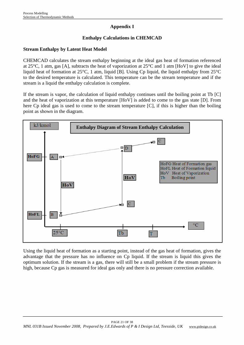
Enthalpy Calculations in CHEMCAD Stream Enthalpy by Latent Heat Model CHEMCAD calculates the stream enthalpy beginning at the ideal gas heat of formation referenced at 25°C, 1 atm, gas [A], subtracts the heat of vaporization at 25°C and 1 atm [HoV] to give the ideal liquid heat of formation at 25°C, 1 atm, liquid [B]. Using Cp liquid, the liquid enthalpy from 25°C to the desired temperature is calculated. This temperature can be the stream temperature and if the stream is a liquid the enthalpy calculation is complete. If the stream is vapor, the calculation of liquid enthalpy continues until the boiling point at Tb [C] and the heat of vaporization at this temperature [HoV] is added to come to the gas state [D]. From here Cp ideal gas is used to come to the stream temperature [C], if this is higher than the boiling point as shown in the diagram.

Using the liquid heat of formation as a starting point, instead of the gas heat of formation, gives the advantage that the pressure has no influence on Cp liquid. If the stream is liquid this gives the optimum solution. If the stream is a gas, there will still be a small problem if the stream pressure is high, because Cp gas is measured for ideal gas only and there is no pressure correction available.

Enthalpy Diagram of Stream Enthalpy Calculation



PAGE 22 OF 38


Appendix I Stream Enthalpy by Equation of State Model The gas enthalpy can also be calculated using an Equation of State. CHEMCAD begins in that case with the ideal gas heat of formation. This has the advantage for the gas phase that the pressure is part of the enthalpy. The gas models are SRK, PR, Lee Kessler, BWRS and others. In the liquid phase these models are not as good as the Cp liquid calculation using the latent heat model. In the case the liquid is highly non-ideal the user should select the Latent Heat model and not an Equation of State for the enthalpy calculation. This is the reason why the thermodynamic Wizard selects NRTL, or UNIQUAC or UNIFAC together only with Latent Heat as the best enthalpy model Calculating the stream enthalpy at 25°C, 1 atm which means the user goes from A to B to C to D to A. this should give the ideal gas heat of formation at 25°C, 1 atm. Theoretically the thermodynamic rules says that, but because of errors in the measured physical properties, which are used here, there will be a small deviation in comparison to the data of the databank if the model is latent heat.



PAGE 23 OF 38


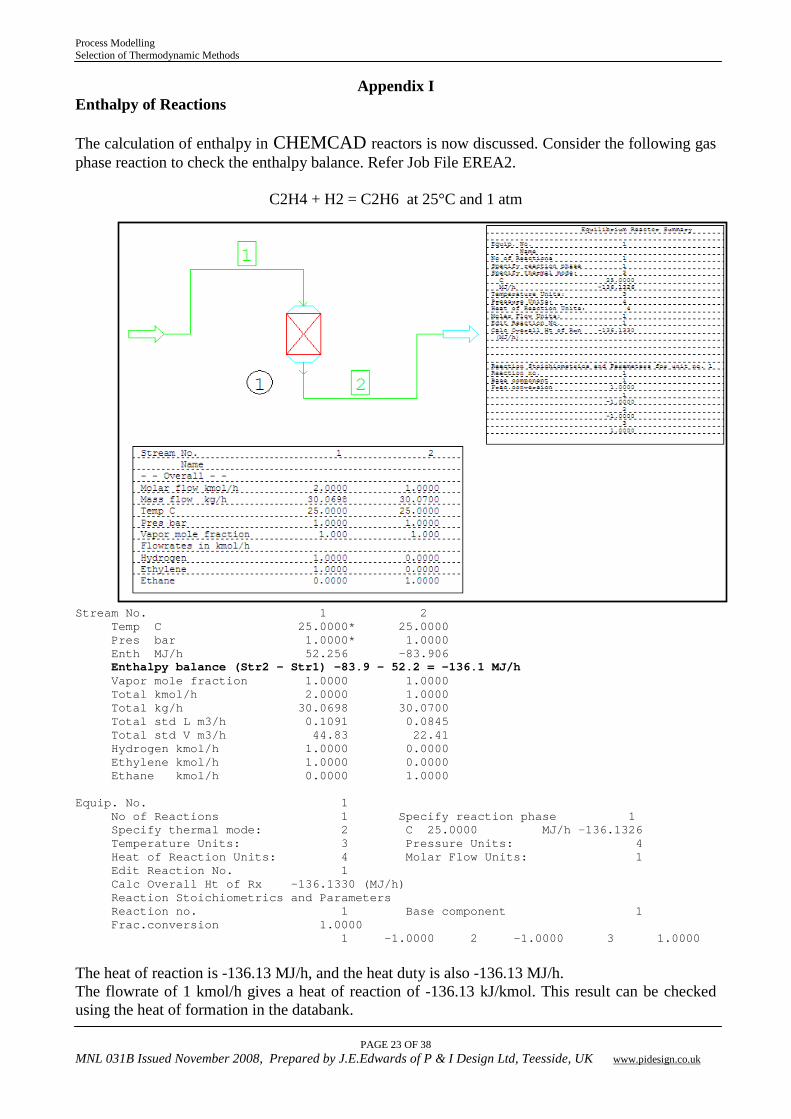
Appendix I Enthalpy of Reactions The calculation of enthalpy in CHEMCAD reactors is now discussed. Consider the following gas phase reaction to check the enthalpy balance. Refer Job File EREA2.

C2H4 + H2 = C2H6 at 25°C and 1 atm

Stream No. 1 2 Temp C 25.0000* 25.0000 Pres bar 1.0000* 1.0000 Enth MJ/h 52.256 -83.906 Enthalpy balance (Str2 – Str1) -83.9 - 52.2 = -136.1 MJ/h Vapor mole fraction 1.0000 1.0000 Total kmol/h 2.0000 1.0000 Total kg/h 30.0698 30.0700 Total std L m3/h 0.1091 0.0845 Total std V m3/h 44.83 22.41 Hydrogen kmol/h 1.0000 0.0000 Ethylene kmol/h 1.0000 0.0000 Ethane kmol/h 0.0000 1.0000 Equip. No. 1 No of Reactions 1 Specify reaction phase 1 Specify thermal mode: 2 C 25.0000 MJ/h -136.1326 Temperature Units: 3 Pressure Units: 4 Heat of Reaction Units: 4 Molar Flow Units: 1 Edit Reaction No. 1 Calc Overall Ht of Rx -136.1330 (MJ/h) Reaction Stoichiometrics and Parameters Reaction no. 1 Base component 1 Frac.conversion 1.0000 1 -1.0000 2 -1.0000 3 1.0000

The heat of reaction is -136.13 MJ/h, and the heat duty is also -136.13 MJ/h. The flowrate of 1 kmol/h gives a heat of reaction of -136.13 kJ/kmol. This result can be checked using the heat of formation in the databank.



PAGE 24 OF 38


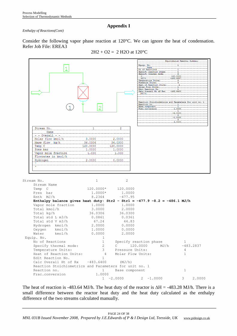
Appendix I Enthalpy of Reactions(Cont) Consider the following vapor phase reaction at 120°C. We can ignore the heat of condensation. Refer Job File: EREA3

2H2 + O2 = 2 H2O at 120°C

Stream No. 1 2 Stream Name Temp C 120.0000* 120.0000 Pres bar 1.0000* 1.0000 Enth MJ/h 8.2364 -477.95 Enthalpy balance gives heat duty: Str2 – Str1 = -477.9 -8.2 = -486.1 MJ/h Vapor mole fraction 1.0000 1.0000 Total kmol/h 3.0000 2.0000 Total kg/h 36.0306 36.0300 Total std L m3/h 0.0861 0.0361 Total std V m3/h 67.24 44.83 Hydrogen kmol/h 2.0000 0.0000 Oxygen kmol/h 1.0000 0.0000 Water kmol/h 0.0000 2.0000 Equip. No. 1 No of Reactions 1 Specify reaction phase 1 Specify thermal mode: 2 C 120.0000 MJ/h -483.2837 Temperature Units: 3 Pressure Units: 4 Heat of Reaction Units: 4 Molar Flow Units: 1 Edit Reaction No. 1 Calc Overall Ht of Rx -483.6400 (MJ/h) Reaction Stoichiometrics and Parameters for unit no. 1 Reaction no. 1 Base component 1 Frac.conversion 1.0000 1 -2.0000 2 -1.0000 3 2.0000 The heat of reaction is -483.64 MJ/h. The heat duty of the reactor is ∆H = -483.28 MJ/h. There is a small difference between the reactor heat duty and the heat duty calculated as the enthalpy difference of the two streams calculated manually.



PAGE 25 OF 38


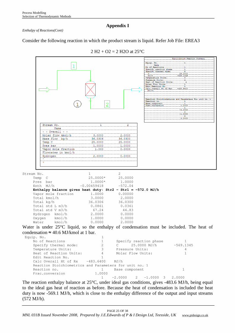
Appendix I Enthalpy of Reactions(Cont) Consider the following reaction in which the product stream is liquid. Refer Job File: EREA3

2 H2 + O2 = 2 H2O at 25°C

Stream No. 1 2 Temp C 25.0000* 25.0000 Pres bar 1.0000* 1.0000 Enth MJ/h -0.00459418 -572.04 Enthalpy balance gives heat duty: Str2 – Str1 = -572.0 MJ/h Vapor mole fraction 1.0000 0.00000 Total kmol/h 3.0000 2.0000 Total kg/h 36.0306 36.0300 Total std L m3/h 0.0861 0.0361 Total std V m3/h 67.24 44.83 Hydrogen kmol/h 2.0000 0.0000 Oxygen kmol/h 1.0000 0.0000 Water kmol/h 0.0000 2.0000 Water is under 25°C liquid, so the enthalpy of condensation must be included. The heat of condensation ≈ 40.6 MJ/kmol at 1 bar. Equip. No. 1 No of Reactions 1 Specify reaction phase 1 Specify thermal mode: 2 C 25.0000 MJ/h -569.1345 Temperature Units: 3 Pressure Units: 4 Heat of Reaction Units: 4 Molar Flow Units: 1 Edit Reaction No. 1 Calc Overall Ht of Rx -483.6400 MJ/h Reaction Stoichiometrics and Parameters for unit no. 1 Reaction no. 1 Base component 1 Frac.conversion 1.0000 1 -2.0000 2 -1.0000 3 2.0000

The reaction enthalpy balance at 25°C, under ideal gas conditions, gives -483.6 MJ/h, being equal to the ideal gas heat of reaction as before. Because the heat of condensation is included the heat duty is now -569.1 MJ/h, which is close to the enthalpy difference of the output and input streams (572 MJ/h).



PAGE 26 OF 38


Appendix I Enthalpy of Reactions(Cont)

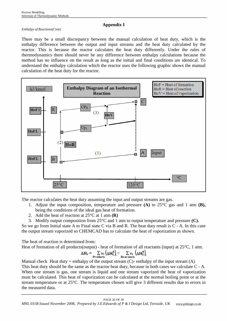
There may be a small discrepancy between the manual calculation of heat duty, which is the enthalpy difference between the output and input streams and the heat duty calculated by the reactor. This is because the reactor calculates the heat duty differently. Under the rules of thermodynamics there should never be any difference between enthalpy calculations because the method has no influence on the result as long as the initial and final conditions are identical. To understand the enthalpy calculation which the reactor uses the following graphic shows the manual calculation of the heat duty for the reactor.

The reactor calculates the heat duty assuming the input and output streams are gas.

1. Adjust the input composition, temperature and pressure (A) to 25°C gas and 1 atm (B), being the conditions of the ideal gas heat of formation.

2. Add the heat of reaction at 25°C at 1 atm (R) 3. Modify output composition from 25°C and 1 atm to output temperature and pressure (C).

So we go from Initial state A to Final state C via B and R. The heat duty result is C - A. In this case the output stream vaporized so CHEMCAD has to calculate the heat of vaporization as shown. The heat of reaction is determined from: Heat of formation of all products(output) - heat of formation of all reactants (input) at 25°C, 1 atm.

( ) ( )HHH 0f itstanacRe

i0f ioductsPr

ir ∆∑ ν−∆∑ ν=∆

Manual check Heat duty = enthalpy of the output stream (C)- enthalpy of the input stream (A) This heat duty should be the same as the reactor heat duty, because in both cases we calculate C - A. When one stream is gas, one stream is liquid and one stream vaporized the heat of vaporization must be calculated. This heat of vaporization can be calculated at the normal boiling point or at the stream temperature or at 25°C. The temperature chosen will give 3 different results due to errors in the measured data.

Enthalpy Diagram of an Isothermal Reaction



PAGE 27 OF 38


Appendix II Thermodynamic Model Synopsis – Vapor Liquid Equilibrium

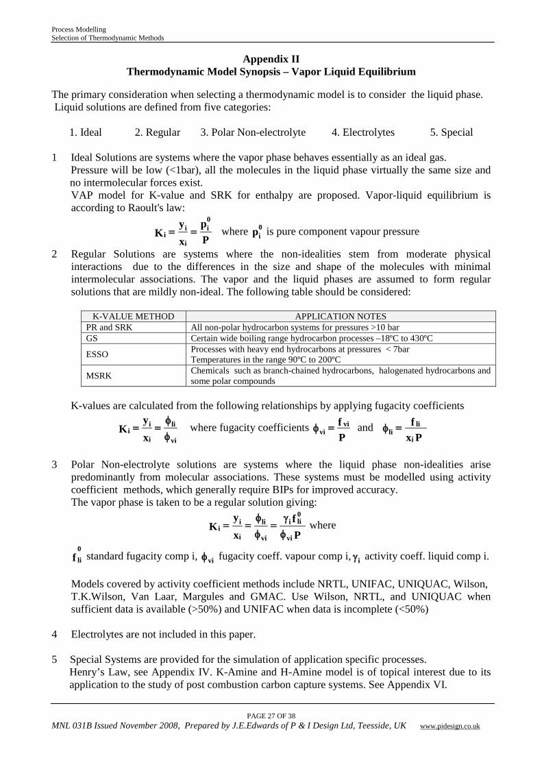
The primary consideration when selecting a thermodynamic model is to consider the liquid phase. Liquid solutions are defined from five categories:

1. Ideal 2. Regular 3. Polar Non-electrolyte 4. Electrolytes 5. Special 1 Ideal Solutions are systems where the vapor phase behaves essentially as an ideal gas. Pressure will be low (<1bar), all the molecules in the liquid phase virtually the same size and

no intermolecular forces exist. VAP model for K-value and SRK for enthalpy are proposed. Vapor-liquid equilibrium is according to Raoult's law:

Pp

xy

K0i

i

ii == where p0

i is pure component vapour pressure

2 Regular Solutions are systems where the non-idealities stem from moderate physical interactions due to the differences in the size and shape of the molecules with minimal intermolecular associations. The vapor and the liquid phases are assumed to form regular solutions that are mildly non-ideal. The following table should be considered:

K-VALUE METHOD APPLICATION NOTES

PR and SRK All non-polar hydrocarbon systems for pressures >10 bar GS Certain wide boiling range hydrocarbon processes –18ºC to 430ºC

ESSO Processes with heavy end hydrocarbons at pressures < 7bar Temperatures in the range 90ºC to 200ºC

MSRK Chemicals such as branch-chained hydrocarbons, halogenated hydrocarbons and some polar compounds

K-values are calculated from the following relationships by applying fugacity coefficients

φφ

==vi

li

i

ii

xy

K where fugacity coefficients Pf vi

vi =φ and Px

fi

lili =φ

3 Polar Non-electrolyte solutions are systems where the liquid phase non-idealities arise

predominantly from molecular associations. These systems must be modelled using activity coefficient methods, which generally require BIPs for improved accuracy. The vapor phase is taken to be a regular solution giving:

Pf

xy

Kvi

0lii

vi

li

i

ii φ

γ=

φφ

== where

f0li standard fugacity comp i, φvi fugacity coeff. vapour comp i, γi activity coeff. liquid comp i.

Models covered by activity coefficient methods include NRTL, UNIFAC, UNIQUAC, Wilson, T.K.Wilson, Van Laar, Margules and GMAC. Use Wilson, NRTL, and UNIQUAC when sufficient data is available (>50%) and UNIFAC when data is incomplete (<50%)

4 Electrolytes are not included in this paper. 5 Special Systems are provided for the simulation of application specific processes.

Henry’s Law, see Appendix IV. K-Amine and H-Amine model is of topical interest due to its application to the study of post combustion carbon capture systems. See Appendix VI.



PAGE 28 OF 38


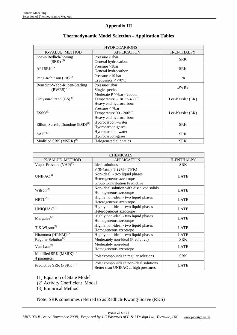
Appendix III

Thermodynamic Model Selection – Application Tables

HYDROCARBONS K-VALUE METHOD APPLICATION H-ENTHALPY

Soave-Redlich-Kwong (SRK) (1)

Pressure >1bar General hydrocarbon SRK

API SRK(1) Pressure >1bar General hydrocarbon SRK

Peng-Robinson (PR)(1) Pressure >10 bar Cryogenics < -70ºC PR

Benedict-Webb-Ruben-Starling (BWRS) (1)

Pressure>1bar Single species BWRS

Grayson-Streed (GS) (1) Moderate P >7bar <200bar Temperature –18C to 430C Heavy end hydrocarbons

Lee-Kessler (LK)

ESSO(3) Pressure < 7bar Temperature 90 - 200ºC Heavy end hydrocarbons

Lee-Kessler (LK)

Elliott, Suresh, Donohue (ESD)(1) Hydrocarbon –water Hydrocarbon-gases SRK

SAFT(1) Hydrocarbon –water Hydrocarbon-gases SRK

Modified SRK (MSRK)(1) Halogenated aliphatics SRK

CHEMICALS K-VALUE METHOD APPLICATION H-ENTHALPY

Vapor Pressure (VAP)(3) Ideal solutions SRK

UNIFAC(2)

P (0-4atm) T (275-475ºK) Non-ideal - two liquid phases Heterogeneous azeotrope Group Contribution Predictive

LATE

Wilson(2) Non-ideal solution with dissolved solids Homogeneous azeotrope LATE

NRTL(2) Highly non-ideal - two liquid phases Heterogeneous azeotrope LATE

UNIQUAC(2) Highly non-ideal - two liquid phases Heterogeneous azeotrope LATE

Margules(2) Highly non-ideal - two liquid phases Homogeneous azeotrope LATE

T.K.Wilson(2) Highly non-ideal - two liquid phases Homogeneous azeotrope LATE

Hiranuma (HRNM)(2) Highly non-ideal - two liquid phases LATE Regular Solution(2) Moderately non-ideal (Predictive) SRK

Van Laar(2) Moderately non-ideal Homogeneous azeotrope LATE

Modified SRK (MSRK)(1) 4 parameter Polar compounds in regular solutions SRK

Predictive SRK (PSRK)(1) Polar compounds in non-ideal solutions Better than UNIFAC at high pressures LATE

(1) Equation of State Model (2) Activity Coefficient Model (3) Empirical Method Note: SRK sometimes referred to as Redlich-Kwong-Soave (RKS)



PAGE 29 OF 38


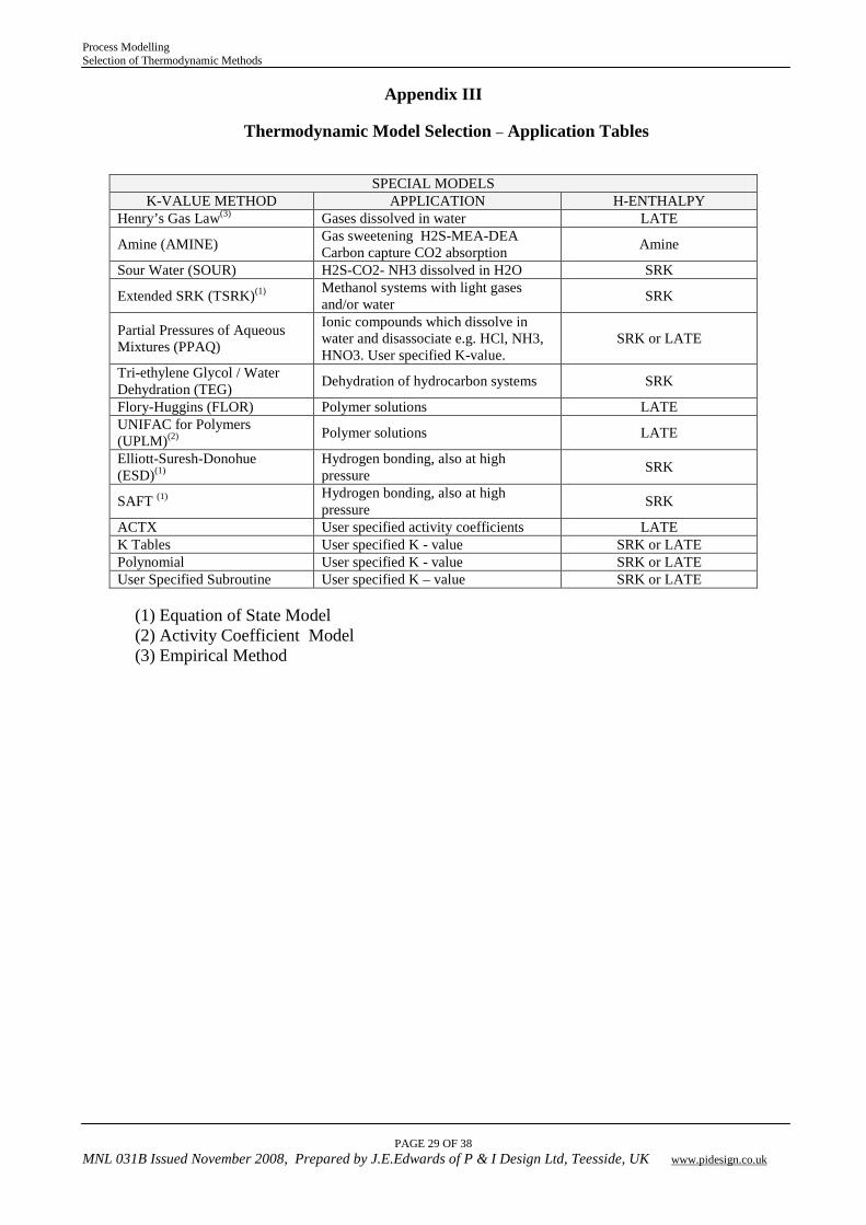
Appendix III

Thermodynamic Model Selection – Application Tables

SPECIAL MODELS K-VALUE METHOD APPLICATION H-ENTHALPY

Henry’s Gas Law(3) Gases dissolved in water LATE

Amine (AMINE) Gas sweetening H2S-MEA-DEA Carbon capture CO2 absorption Amine

Sour Water (SOUR) H2S-CO2- NH3 dissolved in H2O SRK

Extended SRK (TSRK)(1) Methanol systems with light gases and/or water SRK

Partial Pressures of Aqueous Mixtures (PPAQ)

Ionic compounds which dissolve in water and disassociate e.g. HCl, NH3, HNO3. User specified K-value.

SRK or LATE

Tri-ethylene Glycol / Water Dehydration (TEG) Dehydration of hydrocarbon systems SRK

Flory-Huggins (FLOR) Polymer solutions LATE UNIFAC for Polymers (UPLM)(2) Polymer solutions LATE

Elliott-Suresh-Donohue (ESD)(1)

Hydrogen bonding, also at high pressure SRK

SAFT (1) Hydrogen bonding, also at high pressure SRK

ACTX User specified activity coefficients LATE K Tables User specified K - value SRK or LATE Polynomial User specified K - value SRK or LATE User Specified Subroutine User specified K – value SRK or LATE

(1) Equation of State Model (2) Activity Coefficient Model (3) Empirical Method



PAGE 30 OF 38


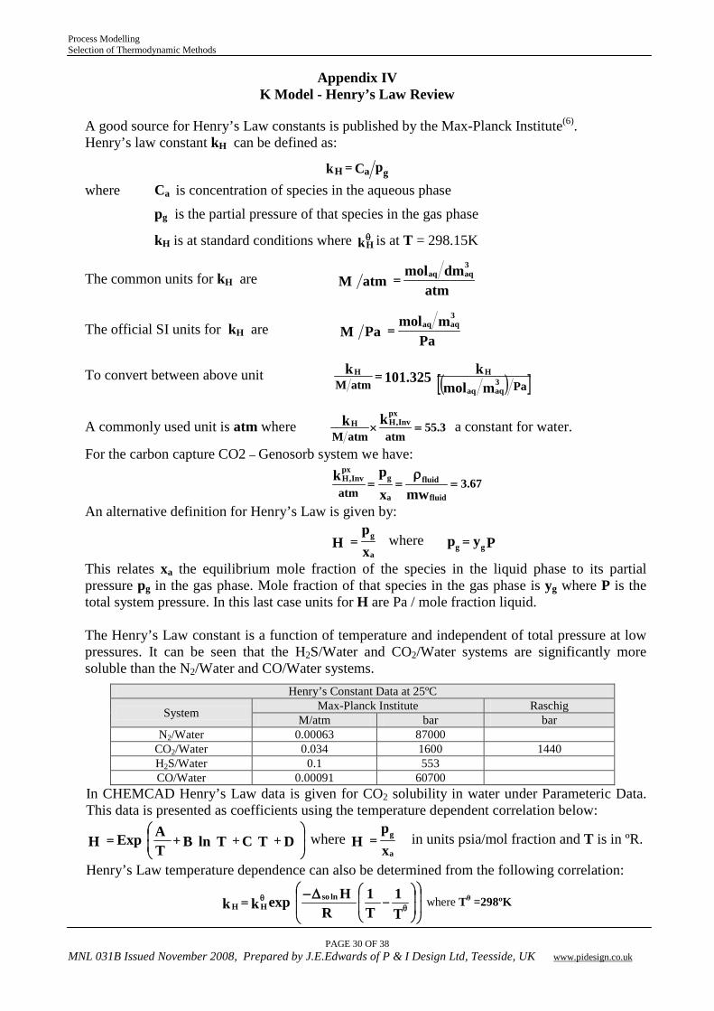
Appendix IV K Model - Henry’s Law Review

A good source for Henry’s Law constants is published by the Max-Planck Institute(6). Henry’s law constant kH can be defined as:

where Ca is concentration of species in the aqueous phase

pg is the partial pressure of that species in the gas phase

kH is at standard conditions where kHθ is at T = 298.15K

The common units for kH are atm

dmmolatmM

3aqaq=

The official SI units for kH are Pa

mmolPaM

3aqaq=

To convert between above unit ( )[ ]PaatmM mmolk325.101k

3aqaq

HH =

A commonly used unit is atm where 3.55atmatmM

kk pxInv,HH =× a constant for water.

For the carbon capture CO2 – Genosorb system we have:

67.3atm mwx

pkfluid

fluid

a

gpx

Inv,H ===ρ

An alternative definition for Henry’s Law is given by:

xp

Ha

g= where Pyp gg =

This relates xa the equilibrium mole fraction of the species in the liquid phase to its partial pressure pg in the gas phase. Mole fraction of that species in the gas phase is yg where P is the total system pressure. In this last case units for H are Pa / mole fraction liquid. The Henry’s Law constant is a function of temperature and independent of total pressure at low pressures. It can be seen that the H2S/Water and CO2/Water systems are significantly more soluble than the N2/Water and CO/Water systems.

Henry’s Constant Data at 25ºC

System Max-Planck Institute Raschig M/atm bar bar

N2/Water 0.00063 87000 CO2/Water 0.034 1600 1440 H2S/Water 0.1 553 CO/Water 0.00091 60700

In CHEMCAD Henry’s Law data is given for CO2 solubility in water under Parameteric Data. This data is presented as coefficients using the temperature dependent correlation below:

+++= DTCTlnBT

AExpH where xp

Ha

g= in units psia/mol fraction and T is in ºR.

Henry’s Law temperature dependence can also be determined from the following correlation:

−= θ

θ ∆−T1

T1

RHexpkk lnso

HH where Tθ =298ºK

pCk gaH =



PAGE 31 OF 38


Appendix V Inert Gases and Infinitely Dilute Solutions

When inert gases, such as CO2, N2, H2 etc., are present with non-ideal chemicals, they present some computational difficulties when using activity models. The K-value is calculated using:

PpV

K iii

ν=

The problem with this method, as far as inert gases are concerned, is that the system is very often operating above the critical point of the pure inert gas. The standard vapor pressure correlation cannot be accurately extrapolated into this region. It is necessary, for the inert gas only, to switch to the Henry's Gas Law method for vapor pressure representation whenever the system temperature is above the critical temperature of a given compound. Each time the vapor pressure is calculated, CHEMCAD compares the critical temperature of each compound to the system temperature. If the system temperature is greater than the critical temperature of one or more of the compounds, then the program will check to see if the Henry's constants are present for the components in question. If the Henry's constants are present, then, for the "inert" compounds only, CHEMCAD will represent the vapor pressure using the Henry's method. All other components will use the regular vapor pressure equation. If the Henry's constants are not present, then the program remains with the regular default vapor pressure method. In certain unusual cases, this approach can cause some numerical difficulties. If the system happens to be operating right in the vicinity of the critical point of one of the components, then it is possible that on one iteration the calculation will be above the critical temperature and on the next it will be below the critical temperature. This will cause the program to switch back and forth between vapor pressure methods, causing numerical discontinuities and non-convergence. This problem can be overcome by telling the program to use the Henry's method globally for certain components. This is done on the K-value screen.

Infinitely Dilute Solutions

The thermodynamic properties of infinitely dilute solutions is acknowledged as being very difficult to predict and systems involving these conditions should always have the results from process simulation work validated by experimental data. The Predictive Soave-Redlich-Kwong (PSRK) equation is a group contribution equation-of-state which combines the SRK and UNIFAC models. This concept makes use of recent developments and has the main advantage that vapour-liquid-equilibrium (VLE) can be predicted for a large number of systems without introducing new model parameters that must be fitted to experimental VLE data. The PSRK equation of state can be used for VLE predictions over a much larger temperature and pressure range than the UNIFAC approach and is easily extended to mixtures containing supercritical compounds. Additional PSRK parameters, including light gases, allows the calculation of gas/gas and gas/ alkane phase equilibrium. The modified UNIFAC model (Dortmund) introduces temperature dependent interaction parameters. This allows a more reliable description of phase behaviour as a function of temperature. The modified UNIFAC (Dortmund) method also uses van der Waals (Q and R) properties which are slightly different than those used in the original UNIFAC method. The main advantages of the modified UNIFAC method are a better description of the temperature dependence and the real behaviour in the dilute region and that it can be applied more reliably for systems involving molecules very different in size.



PAGE 32 OF 38


Appendix VI

Post Combustion Carbon Capture Thermodynamics(8)

In the study of post combustion carbon capture the K-Amine and H-Amine CHEMCAD model has been successfully applied in the study of the absorption and desorption of CO2 in ethanolamine solutions. Aqueous solutions of ethanolamines are used for the reactive absorption of CO2 at atmospheric pressure. The reaction mechanisms are as follows:

2 R-NH2 + CO2 ↔ R-NH3

+ + R-NH-COO-

R-NH2 + CO2 + H2O ↔ R-NH3

+ + HCO3-

In CHEMCAD Amine model uses the Kent Eisenberg method to model the reactions. The following amines are included in the Amine model allowing for further investigation as required.

Diethanolamine (DEA) Monoethanolamine (MEA) Methyl diethanolamine (MDEA)

The chemical reactions in the CO2-Amine system are described by the following reactions:

RR'NH2+ ↔ H+ + RR'NH RR'NCOO + H2O ↔ RR'NH + HCO3 CO2 + H2O ↔ HCO3- + H+ HCO3- ↔ CO3- - + H+ H2O ↔ H+ + OH-

where R and R' represent alcohol groups. The reaction equations are solved simultaneously to obtain the free concentration of CO2. The partial pressure of CO2 is calculated by the Henry's constants and free concentration in the liquid phase. The heat of reaction is also accurately predicted to allow thermal studies to be carried out.

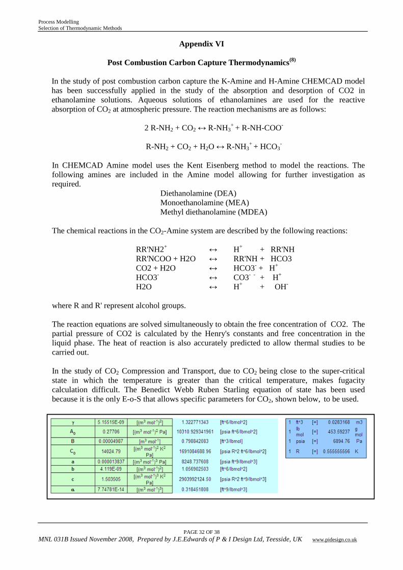
In the study of CO2 Compression and Transport, due to CO2 being close to the super-critical state in which the temperature is greater than the critical temperature, makes fugacity calculation difficult. The Benedict Webb Ruben Starling equation of state has been used because it is the only E-o-S that allows specific parameters for CO2, shown below, to be used.



PAGE 33 OF 38


Appendix VII Thermodynamic Guidance Note

Water - organic Systems 1. If no data is available UNIFAC / UNIFAC LLE is a 'reasonable' model to try. It will predict results that are consistent and it is not unreasonable to trust UNIFAC to be near the results. The more non-ideal the organic the less accurate the results. If using NRTL / UNIQUAC, for other reasons, regress the behaviour of water-organic from UNIFAC. 2. If some data is available, try to validate the UNIFAC results. 3. If some data is available and sufficiently reliable, regress binary interaction parameters (BIPs) without UNIFAC. 4. If working in ppm concentration range regress infinite dilution activity coefficients. Only use UNIFAC if it matched data and there were difficulties regressing the data into NRTL or if wanting to use UNIFAC for some other reason. If there are NRTL/UNIQUAC parameters and some data for validation, use the data to validate BIPs. UNIFAC Group Contribution Method for Hydrocarbons. The two uses of the group contribution method are: 1. To determine pure component properties (Tb, Tc, Pc) for hydrocarbons, 15% accuracy is typical for straight branch, C8 and lower hydrocarbons. See Appendix VIII for predictive methods. 2. Determining non-real binary behaviour due to size and shape of the two molecules. The UNIFAC groups and their interactions are used to calculate the liquid fugacity and to determine the size and shape of a 'part' of the molecule. Regressing BIPs for UNIFAC makes it more useful. When UNIFAC is insufficient for the components you can still use it for the vapor phase, but it fails on the liquid phase and on TPxy behaviour. Interaction parameters between groups dictate the interaction between groups. The overall behaviour is the sum of partial interactions. If the interactions between some of the groups for two components are not available, it means that the groups are being ignored. For example acetic acid and xylene have groups that do not have known interaction parameters, which means that part of the shape of the two is being ignored. There is no H2O group. This means that water is considered to be an ideal circle of ideal gas law size when interacting with another component. H2O is not a sphere, so the liquid fugacity calculation is wrong. The liquid fugacity for xylene-water and xylene-acetic acid is assumed to be 'regular solution,' and the liquid fugacity for xylene-acetic acid is an incomplete result.

UNIQUAC or NRTL with vapor phase association. UNIFAC is not suitable due to lack of interaction parameters for the main groups acetic acid and xylene and there is no water subgroup.



PAGE 34 OF 38



Liquid Liquid Extraction To select a K model that will support the calculation of two liquid phases, set the vapor/ liquid/liquid/solid option on the K value screen. Models NRTL, UNIQUAC, UNIFAC LLE are suitable. It is possible to regress Txy data for a pair of components but be sure to set the K flag V/L/L/S option before regressing, because different regressions are used. Txy data can also be regressed for a ternary system, such as data from a binodal. For a discussion on alpha functions influence on the calculation of activity coefficients for the two liquid phases reference: Smith and Van Ness, “Introduction to Chemical Engineering Thermodynamics”. When using an activity coefficient model to determine equilibrium between two liquid phases, the SCDS UnitOp can be used to determine separation and gamma1, gamma2 show separation regardless of what the two phases are. The calculations for LLE on a stage are the same that would be used for VLE on a stage. There is a special UnitOp, the extractor (EXTR) which is nothing more than an SCDS unit modified to work for two liquid phases rather than one liquid phase and one vapor phase. Whenever your data is expressed as an activity coefficient, you could use the gamma regression. The Flash UnitOp will always bring the vapor and liquid to equilibrium, which is equivalent to a Murphree Efficiency of 1.0. Binodal plots should be obtained for verification of partitioning behaviour. To do a single stage liquid - liquid extraction with Murphree efficiency applied Excel UnitOp can be used to design a special UnitOp. For such low extractions set 2 stages with efficiencies of around 0.2 to 0.3 LLE UnitOp needs a minimum of 2 stages and a single flash gives equilibrium. To generate rectangular coordinate(x-solute in raffinate, y-solute in extract) diagram showing the equilibrium and operating lines export a binodal plot and tower profile plot to Excel, then combine the data. Regressing BIPs for NRTL( K flag set for V/L/L/S) for LLE when using UNIFAC LLE with water present is acceptable provided the water is forming a second phase, it is always best to check with data though. General Rules Liquid phase water with “anything else” most times use NRTL. You can regress NRTL BIPs for the other components from UNIQUAC or UNIFAC if you don't have NRTL bips. SRK is an equation of state which uses the accentric factor of a component and some 'general curve fit' parameters from “lots of lab studies” to calculate the fugacity on the basis that both molecules in the binary mixture are spheres, the only difference is how big they are. Again, water is not a sphere and it's non-ideal behavior stems from its shape as well as its size. Peng Robinson and SRK Equations of State are good for non-water mixtures of gases and excellent for light gases and refrigerants. However they cannot handle two phase water but are good for two phase hydrocarbons. Great for non-polar, not so good for polar solutions.



PAGE 35 OF 38



You can regress a BIP for binary behaviour which is really just a mixing bip (Kij=Ki/Kj=A+B*T) If using an EOS with water there are two methods: 1. Use NRTL and turn on either Vapor Fugacity Correction (use SRK for the vapor phase fugacity) 2. Use NRTL with Henry's component set for near supercritical light gases. Activity coefficients are good for polar solutions, if you have activity coefficient bips regressed. UNIFAC is good for hydrocarbons, even polar hydrocarbons, if you have subgroups. Not good if there is a liquid phase. Batch Distillation For a multi-component organic-water system, with regressed vapor pressure data, the first choice would be NRTL. An equation of state is unsuitable unless the accentric factor is tuned; more details are available in the Help section. When using the pseudo binary method to correlate the behaviour of a mixture based on the behaviour of pairs of components to each other, the situation may occur where this isn't valid (phase partitioning, ternary azeotropes) because the ternary, quaternary system behaves significantly different than pseudo binary predicts. When guessing BIPs from UNIFAC this can be a danger. When uncertain of BIPs it is not wise to make column specifications based on composition. VLE data is available from DECHEMA. Regression of User Component Data Enter the User Component screen for the physical property to be regressed and enter the upper and lower limit temperatures with the relevant physical property data in the correct units. Note the regression equation on this “screen is not set in stone” and may be changed. Density is particularly difficult to achieve a regression and changing the equation to 100 the straight line function may help as density approximates to this over a narrow range. Successful results can be achieved with two data points only, but ensure that data at 0°C is not entered. Key data points can be weighted e.g. 10000 to force regression through the point. Pseudo component method is for hydrocarbons to calculate Tc and Pc ie assumes component is a hydrocarbon. Use pseudo components for hydrocarbons. If it is not a hydrocarbon use Joback or UNIFAC depending on the compound and do not enter an SG; note this should have no effect on pure component regressions. If user component below mp at 60ºF do not enter SG. Joback is easier to get halogens into, more flexible groups, but UNIFAC does a better job characterizing Poly Cyclic compounds. When using UNIFAC if error message saying "UNIFAC groups unspecified for component" there are no groups and the activity coefficient for that component is set = 1 ie basis will be taken as ideal behaviour The most important thing is to try it several ways, and understand that these estimation methods DO NOT replace the need for actual lab data on your compound. Once laboratory data is available the issue is resolved.



PAGE 36 OF 38


APPENDIX VIII

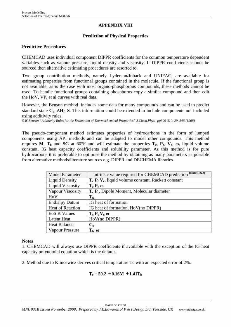
Prediction of Physical Properties Predictive Procedures

CHEMCAD uses individual component DIPPR coefficients for the common temperature dependent variables such as vapour pressure, liquid density and viscosity. If DIPPR coefficients cannot be sourced then alternative estimating procedures are resorted to.

Two group contribution methods, namely Lyderson/Joback and UNIFAC, are available for estimating properties from functional groups contained in the molecule. If the functional group is not available, as is the case with most organo-phosphorous compounds, these methods cannot be used. To handle functional groups containing phosphorus copy a similar compound and then edit the HoV, VP, et al curves with real data.

However, the Benson method includes some data for many compounds and can be used to predict standard state Cp, ∆Hf, S. This information could be extended to include components not included using additivity rules. S.W.Benson “Additivity Rules for the Estimation of Thermochemical Properties” J.Chem.Phys., pp309-310, 29, 546 (1968)

The pseudo-component method estimates properties of hydrocarbons in the form of lumped components using API methods and can be adapted to model other compounds. This method requires M, Tb and SG at 60°F and will estimate the properties Tc, Pc, Vc, ω, liquid volume constant, IG heat capacity coefficients and solubility parameter. As this method is for pure hydrocarbons it is preferable to optimise the method by obtaining as many parameters as possible from alternative methods/literature sources e.g. DIPPR and DECHEMA libraries.

Model Parameter Intrinsic value required for CHEMCAD prediction (Notes 1&2)

Liquid Density Tc Pc Vc, liquid volume constant, Rackett constant Liquid Viscosity Tc Pc ω Vapour Viscosity Tc Pc, Dipole Moment, Molecular diameter HoV Tb Enthalpy Datum IG heat of formation Heat of Reaction IG heat of formation, HoV(no DIPPR) EoS K Values Tc Pc Vc ω Latent Heat HoV(no DIPPR) Heat Balance Cp Vapour Pressure Tb ω

Notes 1. CHEMCAD will always use DIPPR coefficients if available with the exception of the IG heat capacity polynomial equation which is the default. 2. Method due to Klincewicz derives critical temperature Tc with an expected error of 2%.

T41.1M16.02.50T bc +−=



PAGE 37 OF 38


APPENDIX VIII

Prediction of Physical Properties

Component Properties for Process Simulation:- For modelling reactions in the liquid phase the following component properties are required:-

• Chemical formula. • Molecular weight M. • Liquid heat capacity Cp.

Two data points in operating range preferred. Less important if reaction is isothermal. If the problem component is very dilute the solution Cp can be used since enthalpy is a partial molar property and if xi is small you can assume the solution Cp will not be significantly influenced.

• Specific gravity at 20°C. If the problem component is very dilute the solution liquid density ρf can be used.

• Ideal Gas (IG) Heat of Formation or Heat of Reaction. For component flashing process:-

• Normal boiling point Tb • Heat of Vaporisation (HoV) at normal boiling point hfg • The HoV at other temperatures can be found by correlation from HoV at Tb but this is

not the most accurate prediction. HoV can be estimated from Tr and ω • Accentric factor ω • Vapour pressure can be estimated using Tb, Tc and M using Gomez Thodos method but

regression from several data points is to be preferred. For mixed phase process:-

• VLE data of the component in the reaction mixture

It is doubtful that Ideal will apply, and UNIFAC VLE will also not suitable for this case.

For solids formation:-

• Solubility data over operating temperature range



PAGE 38 OF 38


APPENDIX VIII

Prediction of Physical Properties

Useful References for Physical Property Predictions

• S. W. Benson, F.R. Cruickskank, D.M. Golden. G.R. Haugon, H.E. O’Neal, A.S. Rodgers, R. Shaw, and R. Walsh, Chem. Rev. 69, 279-324 (1969).

• S. W. Benson, ‘Thermochemical Kinetics, 2nd Edition, ‘John Wiley and Sons, New York (1976).

• S. W. Benson and J. H. Buss, J. Chem. Phys. 19, 279 (1968).

• F. N. Fritsch and R. E. Carlson, SIAM J. Numerical Analysis 17, 258-46 (1980).

• F. N. Fritsch and J. Butland, UCRL-85104, Lawrence Livermore Laboratory, October, 1980.

• B. K. Harrison and W. H. Seaton, ‘A solution to the missing group problem for estimation of ideal gas heat capacities,’ Ind. Eng. Chem. Res. 27, 1536-40 (1988).

• J. E. Hurst, Jr., and B. K. Harrison, ‘Estimation of liquid and solid heat capacities using a modified Kopp’s rule,’ Chem. Eng. Commun, 112, 21-30 (1992).

• C. D. Ratkey and B. K. Harrison, ‘Prediction of enthalpies of formation for ionic compound,’ Ind. Eng. Chem. Res. 31 (10), 2362-9 (1992).

• W. H. Seaton, ‘Group Contribution Method for Predicting the Potential of a chemical composition to cause an explosion, J. Chem. Educ. 66, A137-40 (1989).

• C. A. Davies, D .J. Frurip, E. Freedman, G.R. Hertel, W.H. Seaton, and D. N. Treweek, ‘CHETAH 4.4: the ASTM chemical thermodynamic and energy release program,’ 2nd edition, ASTM Publication DS 51A (1990).

• J. R. Downey, D. J. Frurip, M. S. LaBarge, A. N. Syverud, N. K. Grant, M. D. Marks, B. K. Harrison, W.H. Seaton, D. N. Treweek, and T. B. Selover, ‘CHETAH 7.0 Users Manuals: the ASTM Computer program for chemical thermodynamic and energy release evaluation,’ NIST Special Database 16, ASTM, ISBN 0-8031-1800-7, Philadelphia, PA (1994).

• Gustin, J.L., "Thermal Stability Screening and Reaction Calorimetry. Application to Runaway Reaction Hazard Assessment at Process Safety Management, J. Loss Prev. Process Inc., Vol. 6, No. 5, (1993).

• Ching-Li Huang, Dr. Keith Harrison, Jeffry Madura, and Jan Dolfing, Gibbs Free Energies of Formation of PCDDS: Evaluation of Estimation Methods and Application for Predicting Dehalogenation Pathways, Environmental Toxicology and Chemistry, Vo. 15, No. 6, pp. 824-836, 1996.


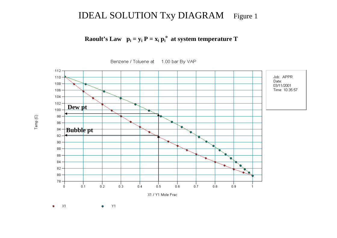
IDEAL SOLUTION Txy DIAGRAM Figure 1

Bubble pt

Dew pt

Raoult’s Law pi = yi P = xi pio at system temperature T

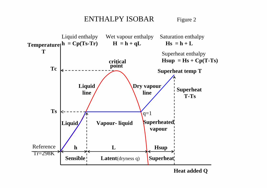
ENTHALPY ISOBAR Figure 2

Temperature

T

Heat added Q

critical

Ts

Tc

Vapour- liquid Liquid

point

Dry vapour line

h L

Liquid line

Hsup

Superheat temp T

q=1 Superheated

vapour

Reference Tr=298K

Liquid enthalpy h = Cp(Ts-Tr)

Saturation enthalpy Hs = h + L

Wet vapour enthalpy H = h + qL

Superheat enthalpy Hsup = Hs + Cp(T-Ts)

Sensible Latent(dryness q) Superheat

Superheat T-Ts

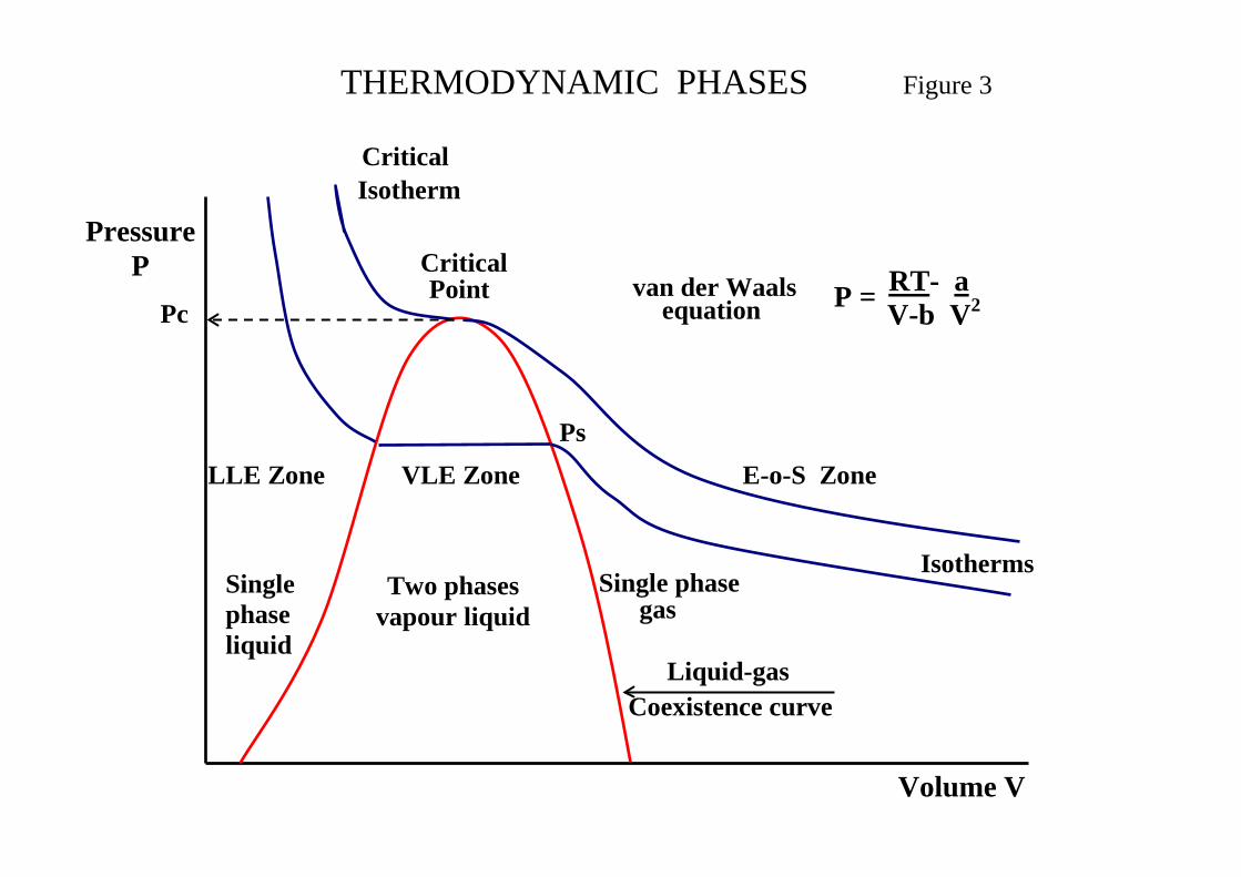
THERMODYNAMIC PHASES Figure 3

Critical

Isotherms

Pressure P

Volume V

Single phase

RT- a V-b V2

van der Waals

Ps

Pc

VLE Zone

Two phases vapour liquid gas

Single phase liquid

LLE Zone

Liquid-gas Coexistence curve

P = equation

E-o-S Zone

Isotherm Critical Point

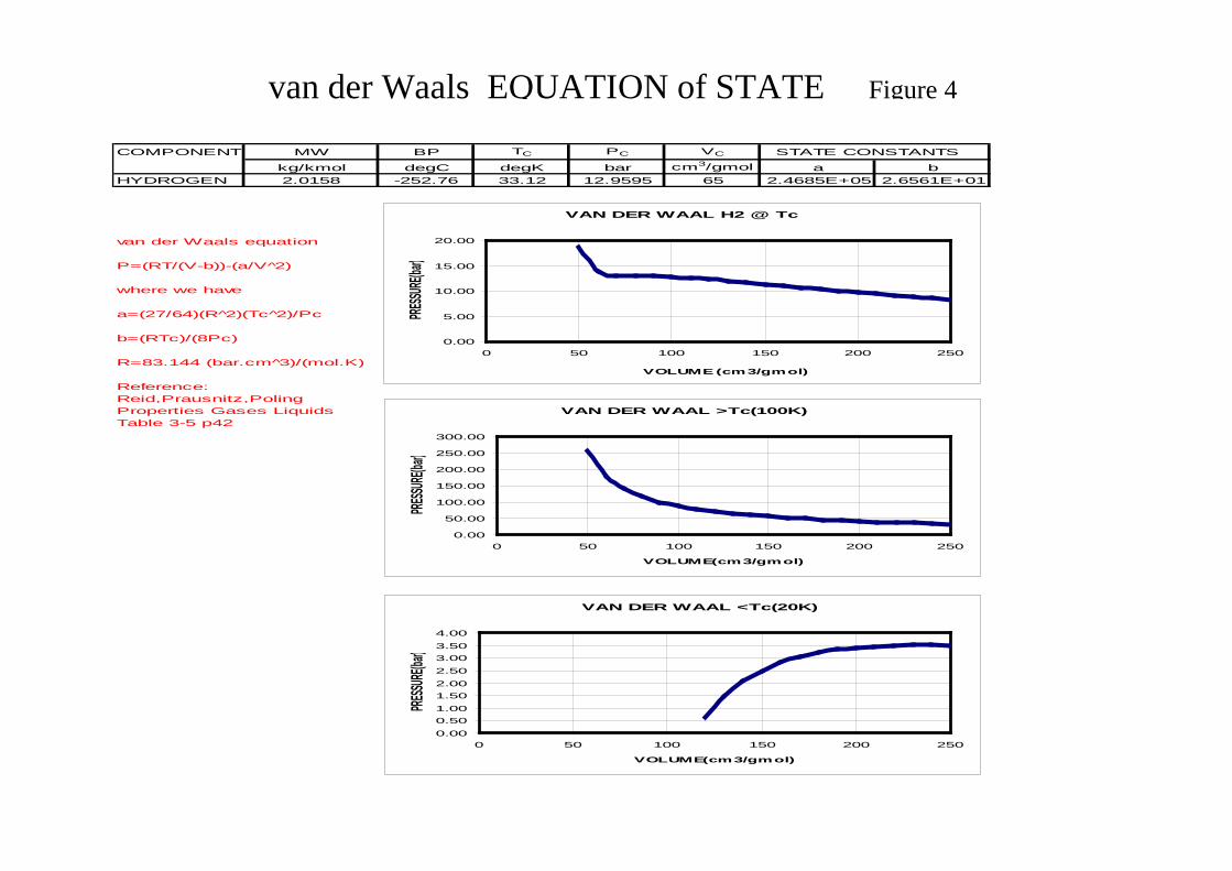
COMPONENT MW BP TC PC VC STATE CONSTANTS

kg/kmol degC degK bar cm3/gmol a bHYDROGEN 2.0158 -252.76 33.12 12.9595 65 2.4685E+05 2.6561E+01

van der Waals equation

P=(RT/(V-b))-(a/V 2̂)

where we have

a=(27/64)(R 2̂)(Tc 2̂)/Pc

b=(RTc)/(8Pc)

R=83.144 (bar.cm 3̂)/(mol.K)

Reference:Reid,Prausnitz,PolingProperties Gases LiquidsTable 3-5 p42

VAN DER WAAL H2 @ Tc

0.00

5.00

10.00

15.00

20.00

0 50 100 150 200 250

VOLUME (cm3/gmol)

PRESSU

RE(bar

)VAN DER WAAL >Tc(100K)

0.00

50.00

100.00

150.00

200.00

250.00

300.00

0 50 100 150 200 250

VOLUME(cm3/gmol)

PRESSU

RE(bar

)

VAN DER WAAL <Tc(20K)

0.000.501.001.502.002.503.003.504.00

0 50 100 150 200 250

VOLUME(cm3/gmol)

PRESSU

RE(bar

)

van der Waals EQUATION of STATE Figure 4

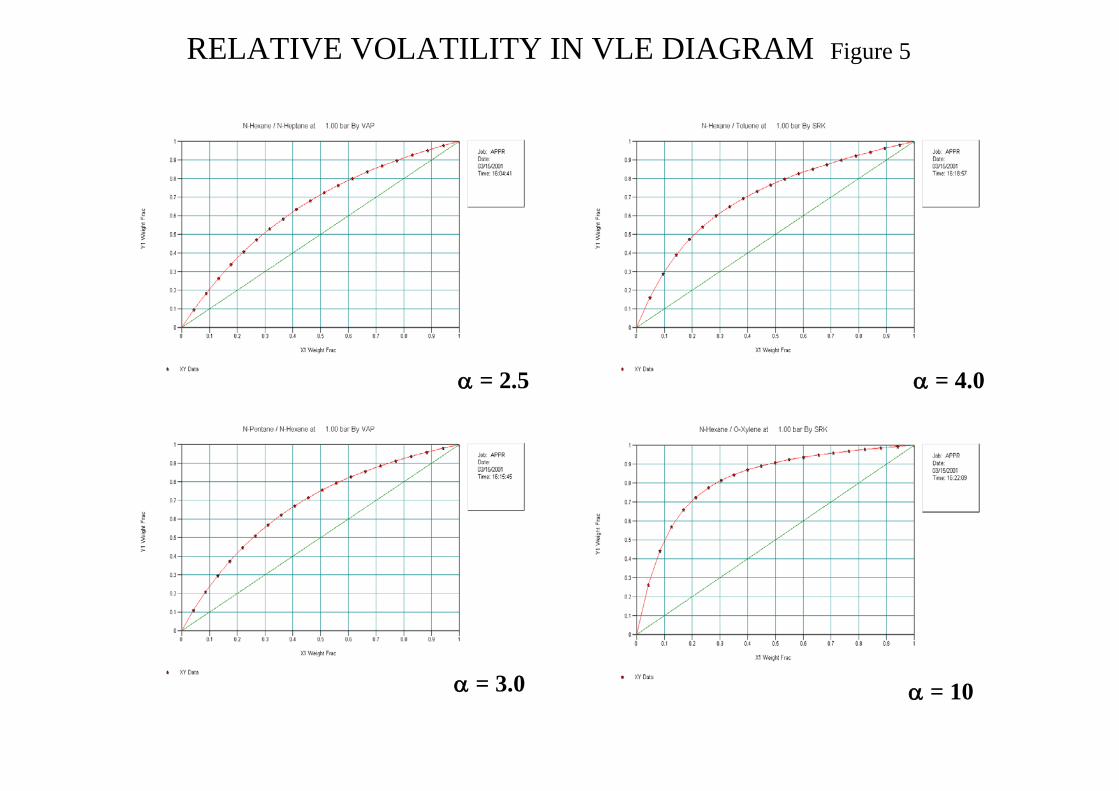
RELATIVE VOLATILITY IN VLE DIAGRAM Figure 5

α = 2.5

α = 10

α = 4.0

α = 3.0

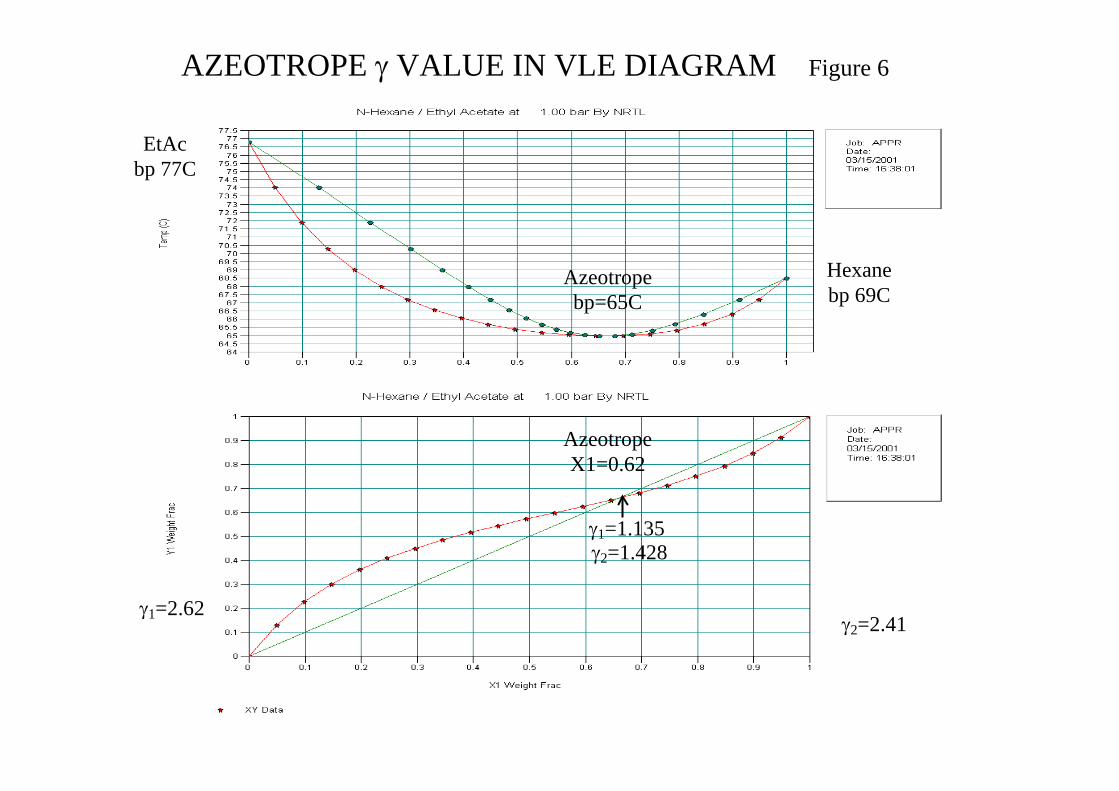
AZEOTROPE γ VALUE IN VLE DIAGRAM Figure 6

Hexane bp 69C

EtAc bp 77C

Azeotrope X1=0.62

Azeotrope bp=65C

γ1=2.62 γ2=2.41

γ2=1.428 γ1=1.135

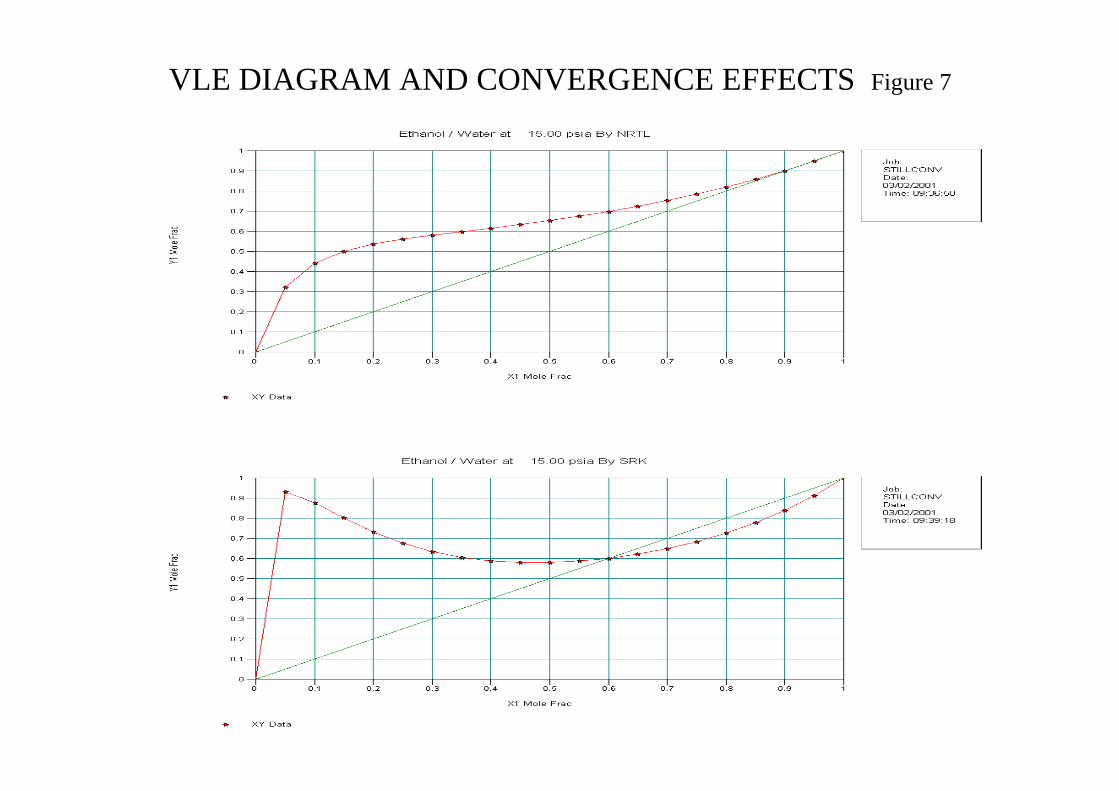
VLE DIAGRAM AND CONVERGENCE EFFECTS Figure 7

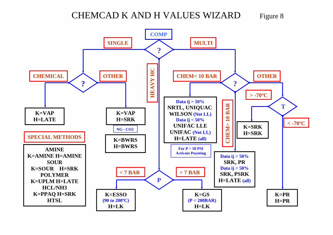
CHEMCAD K AND H VALUES WIZARD Figure 8

?

?

P

Data ij > 50% SRK, PR

Data ij < 50% SRK, PSRK

H=LATE (all)

?

K=VAP H=SRK

K=VAP H=LATE

SINGLE

CHEMICAL OTHER

MULTI

CHEM< 10 BAR OTHER

CH

EM

> 10

BA

R

< 7 BAR

HE

AV

Y H

C

> 7 BAR

AMINE K=AMINE H=AMINE

SOUR K=SOUR H=SRK

POLYMER K=UPLM H=LATE

HCL/NH3 K=PPAQ H=SRK

HTSL

K=ESSO (90 to 200ºC)

H=LK

K=GS (P < 200BAR)

H=LK

Data ij > 50% NRTL, UNIQUAC WILSON (Not LL)

Data ij < 50% UNIFAC LLE

UNIFAC (Not LL) H=LATE (all)

T

K=PR H=PR

K=SRK H=SRK

> -70ºC

SPECIAL METHODS

COMP

K=BWRS H=BWRS

NG - CO2

For P > 50 PSI Activate Poynting

< -70ºC

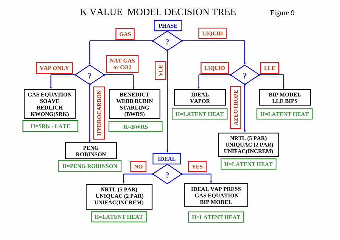
K VALUE MODEL DECISION TREE Figure 9

?

?

? IDEAL VAP PRESS GAS EQUATION

BIP MODEL

BIP MODEL LLE BIPS

NRTL (5 PAR) UNIQUAC (2 PAR) UNIFAC(INCREM)

?

PENG ROBINSON

BENEDICT WEBB RUBIN

STARLING (BWRS)

GAS EQUATION SOAVE

REDLICH KWONG(SRK)

GAS

VAP ONLY NAT GAS

or CO2

LIQUID

LIQUID LLE

HY

DR

OC

AR

BO

N

AZ

EO

TR

OPE

NO V

LE

YES

NRTL (5 PAR) UNIQUAC (2 PAR) UNIFAC(INCREM)

H=LATENT HEAT

H=LATENT HEAT H=LATENT HEAT

H=LATENT HEAT

H=BWRS

H=PENG ROBINSON

H=SRK - LATE

IDEAL VAPOR

PHASE

IDEAL H=LATENT HEAT

Documents

P & I Design Ltd - CHEMCAD is a suite of chemical process ... · 1 Ideal Solution Txy Diagram ... R.C. Reid, J.M. Prausnitz, B.E. Poling,“The Properties of Gases ... based on a