Embed Size (px)
Citation preview
The Center for Satellite and Hybrid Communication Networks is a NASA-sponsored Commercial SpaceCenter also supported by the Department of Defense (DOD), industry, the State of Maryland, the University
of Maryland and the Institute for Systems Research. This document is a technical report in the CSHCNseries originating at the University of Maryland.
Web site http://www.isr.umd.edu/CSHCN/
PH.D. THESIS
Routing and Scheduling Algorithms in Resource-Limited Wireless Multi-Hop Networks
by Anastassios MichailAdvisor: Anthony Ephremides
CSHCN PhD 2001-1(ISR PhD 2001-1)
ABSTRACT
Title of Dissertation: Routing and Scheduling Algorithms in Resource-limited
Wireless Multi-hop Networks
Anastassios Michail, Doctor of Philosophy, 2001
Dissertation directed by: Professor Anthony Ephremides
Department of Electrical and Computer Engineering
The recent advances in the area of wireless networking present novel oppor-
tunities for network operators to expand their services to infrastructure-less wire-
less systems. Such networks, often referred to as ad-hoc or multi-hop or peer-
to-peer networks, require architectures which do not necessarily follow the cellular
paradigm. They consist of entirely wireless nodes, fixed and/or mobile, that require
multiple hops (and hence relaying by intermediate nodes) to transmit their mes-
sages to the desired destinations. The distinguishing features of such all-wireless
network architectures give rise to new trade-offs between traditional concerns in
wireless communications (such as spectral efficiency, and energy conservation) and
the notions of routing, scheduling and resource allocation. The purpose of this
work is to identify and study some of these novel issues, propose solutions in the
context of network control and evaluate the usual network performance measures
as functions of the new trade-offs.
To these ends, we address first the problem of routing connection-oriented
traffic with energy efficiency in all-wireless multi-hop networks. We take advantage
of the flexibility of wireless nodes to transmit at different power levels and define a
framework for formulating the problem of session routing from the perspective of
energy expenditure. A set of heuristics are developed for determining end-to-end
unicast paths with sufficient bandwidth and transceiver resources, in which nodes
use local information in order to select their transmission power and bandwidth
allocation. We propose a set of metrics that associate each link transmission with a
cost and consider both the cases of plentiful and limited bandwidth resources, the
latter jointly with a set of channel allocation algorithms. Performance is measured
by call blocking probability and average consumed energy and a detailed simulation
model that incorporates all the components of our algorithms has been developed
and used for performance evaluation of a variety of networks.
In the sequel, we propose a ”blueprint” for approaching the problem of link
bandwidth management in conjunction with routing, for ad-hoc wireless networks
carrying packet-switched traffic. We discuss the dependencies between routing,
access control and scheduling functions and propose an adaptive mechanism for
solving the capacity allocation (at both the node-level and the flow-level) and
the route assignment problems, that manages delays due to congestion at nodes
and packet loss due to error prone wireless links, to provide improved end-to-end
delay/throughput. The capacity allocations to the nodes and flows and the route
assignments are iterated periodically and the adaptability of the proposed approach
allows the network to respond to random channel error bursts and congestion

arising from bursty and new flows.
Routing and Scheduling Algorithms in Resource-limited Wireless Multi-hop Networks
by
Anastassios Michail
Dissertation submitted to the Faculty of the Graduate School of theUniversity of Maryland, College Park in partial fulfillment
of the requirements for the degree ofDoctor of Philosophy
2001
Advisory Committee:
Professor Anthony Ephremides, Chairman/AdvisorDr. M. Scott CorsonProfessor Evaggelos GeraniotisProfessor Steven MarcusProfessor A. Udaya Shankar

c©Copyright by
Anastassios Michail
2001

ACKNOWLEDGEMENTS
I would like to express my gratitude to my advisor, Professor Anthony
Ephremides. His valuable support and exceptional guidance through-
out my graduate school years have helped me achieve much more than
I had expected when I came to Maryland. He made me believe in
myself and without his persistence and encouragement I would have
never felt confident to pursue the Doctoral program. I gained a lot of
knowledge and valuable experience while working with him. His unique
personality turned every single moment of interaction into a learning
experience.
I am thankful to the members of the dissertation committee, Dr. Scott
Corson and Professors Evaggelos Geraniotis, Steve Marcus and Udaya
Shankar for kindly reviewing my dissertation and consenting to serve on
the defense committee. I also wish to specially thank Professors Steve
Marcus and Leandros Tassiulas for their valuable comments and advice
on my research proposal. They provided me with constructive criticism
that helped improve my work. Unfortunately Professor Tassiulas was
on leave at the time of the defense and could not participate in the
committee.
ii

I had the opportunity to work closely on one of the research problems
with Dr. Deepak Ayyagari. Deepak has been a very good friend and
having known each other very well made it easier to collaborate. I wish
to thank him for several discussions we had and for his valuable help.
It is extremely hard to find words that express my gratitude to my
parents Tolis and Dora and my sister Nadia for their invaluable help
over all these years. They gave me courage and strength whenever
I needed it and supported me in every possible way throughout the
course of my studies. I am also grateful to Marianna who has been very
supportive and patient all this time and with her love and dedication
she gave me the extra courage and confidence I needed to accomplish
this work.
Throughout the six years I spent in Maryland I had the chance to meet
a lot of new friends. They made life easier and I wish them all luck
in their future plans. It would be a very long list if I had to mention
names but I ought to express my special thanks to all my roommates
for sharing a house with me most of these years and for bearing with
me during both the good and the bad times.
Least, but not last, I wish to thank my fellow graduate students, all
my officemates and the members of the Systems Engineering and Inte-
gration Lab for creating a pleasant working environment.
This work wouldn’t have been possible without the financial support of
the Institute for Systems Research. Funding was provided by the Ad-
vanced Telecommunications/Information Distribution Research Pro-
gram (ATIRP) Consortium sponsored by the U.S. Army Research Lab-
iii

oratory under Cooperative Agreement DAAL01-96-2-0002.
iv

TABLE OF CONTENTS
List of Tables ix
List of Figures x
1 Introduction 1
1.1 Summary and organization of dissertation . . . . . . . . . . . . . . 5
2 Energy-Efficient Routing of Connection-Oriented Traffic, Part I:
Limited Transceiver Resources 7
2.1 Motivation and objectives . . . . . . . . . . . . . . . . . . . . . . . 7
2.1.1 Related work . . . . . . . . . . . . . . . . . . . . . . . . . . 9
2.1.2 Research contributions . . . . . . . . . . . . . . . . . . . . . 10
2.1.3 Outline of the chapter . . . . . . . . . . . . . . . . . . . . . 12
2.2 Wireless network model . . . . . . . . . . . . . . . . . . . . . . . . 13
2.3 Proposed algorithms . . . . . . . . . . . . . . . . . . . . . . . . . . 16
2.3.1 Overview . . . . . . . . . . . . . . . . . . . . . . . . . . . . 16
2.3.2 Link metrics . . . . . . . . . . . . . . . . . . . . . . . . . . . 18
2.4 Simulation model . . . . . . . . . . . . . . . . . . . . . . . . . . . . 24
2.5 Performance results . . . . . . . . . . . . . . . . . . . . . . . . . . . 26
2.5.1 Blocking probability (Pb) . . . . . . . . . . . . . . . . . . . . 26
v

2.5.2 Average energy per session (Es) . . . . . . . . . . . . . . . . 31
2.5.3 Effect of node density on performance . . . . . . . . . . . . 33
2.5.4 Effect of average node degree on performance . . . . . . . . 39
2.5.5 Energy versus blocking trade-off and yardstick (Y ) perfor-
mance . . . . . . . . . . . . . . . . . . . . . . . . . . . . . . 42
2.5.6 Effect of receive and processing power on energy consumption 43
2.5.7 Network “lifetime” . . . . . . . . . . . . . . . . . . . . . . . 46
2.6 Conclusions . . . . . . . . . . . . . . . . . . . . . . . . . . . . . . . 50
3 Energy-Efficient Routing of Connection-Oriented Traffic, Part II:
Limited Bandwidth Resources 53
3.1 Introduction . . . . . . . . . . . . . . . . . . . . . . . . . . . . . . . 53
3.2 Interference model . . . . . . . . . . . . . . . . . . . . . . . . . . . 58
3.3 Algorithmic considerations . . . . . . . . . . . . . . . . . . . . . . . 61
3.4 Heuristic algorithms . . . . . . . . . . . . . . . . . . . . . . . . . . 65
3.4.1 Link metrics for determining minimum cost path . . . . . . 65
3.4.2 Frequency allocation algorithms . . . . . . . . . . . . . . . . 67
3.5 Exhaustive search mechanisms . . . . . . . . . . . . . . . . . . . . . 71
3.5.1 Complete exhaustive search implementation (ExSrch) . . . . 71
3.5.2 Exhaustive search of minimum-cost path (ESMP) . . . . . . 73
3.6 Performance analysis . . . . . . . . . . . . . . . . . . . . . . . . . . 74
3.6.1 Comparison of frequency allocation heuristics versus exhaus-
tive search mechanisms . . . . . . . . . . . . . . . . . . . . . 75
3.6.2 Performance comparison of LLG versus MCLF for random
topologies . . . . . . . . . . . . . . . . . . . . . . . . . . . . 80
vi
3.6.3 Performance characteristics of link metrics for use with link-
by-link greedy frequency allocation scheme . . . . . . . . . . 83
3.7 Conclusions . . . . . . . . . . . . . . . . . . . . . . . . . . . . . . . 87
4 A “Blueprint” towards an Integrated Scheduling, Access Control
and Routing Scheme in Wireless Ad-Hoc Networks 91
4.1 Motivation . . . . . . . . . . . . . . . . . . . . . . . . . . . . . . . . 91
4.2 Background . . . . . . . . . . . . . . . . . . . . . . . . . . . . . . . 94
4.2.1 Scheduling disciplines for wire-line networks . . . . . . . . . 94
4.2.2 Scheduling disciplines for cellular wireless networks . . . . . 98
4.2.3 Scheduling in wireless LANs . . . . . . . . . . . . . . . . . . 101
4.2.4 Scheduling in wireless multi-hop networks . . . . . . . . . . 102
4.3 A unified approach to scheduling, access-control and routing in ad-
hoc networks . . . . . . . . . . . . . . . . . . . . . . . . . . . . . . 103
4.3.1 Overview . . . . . . . . . . . . . . . . . . . . . . . . . . . . 103
4.3.2 Proposed model . . . . . . . . . . . . . . . . . . . . . . . . . 104
4.3.3 Link error adjusted rate (LEAR) measure . . . . . . . . . . 107
4.3.4 Routing updates . . . . . . . . . . . . . . . . . . . . . . . . 109
4.4 Description of algorithms . . . . . . . . . . . . . . . . . . . . . . . . 110
4.4.1 Notation . . . . . . . . . . . . . . . . . . . . . . . . . . . . . 110
4.4.2 Node-level scheduling . . . . . . . . . . . . . . . . . . . . . . 111
4.4.3 Flow-level scheduling . . . . . . . . . . . . . . . . . . . . . . 112
4.4.4 Routing . . . . . . . . . . . . . . . . . . . . . . . . . . . . . 113
4.5 Performance results . . . . . . . . . . . . . . . . . . . . . . . . . . . 114
4.5.1 Network and traffic patterns . . . . . . . . . . . . . . . . . . 114
4.5.2 Performance measures . . . . . . . . . . . . . . . . . . . . . 115
vii
4.5.3 Simulation results . . . . . . . . . . . . . . . . . . . . . . . . 115
4.6 Future directions . . . . . . . . . . . . . . . . . . . . . . . . . . . . 116
5 Conclusions 119
Appendix 122
A Simulation model for energy-efficient routing algorithms 122
Bibliography 132
viii
LIST OF TABLES
2.1 Average number of hops and standard deviation per admitted ses-
sion for N = 20 . . . . . . . . . . . . . . . . . . . . . . . . . . . . . 31
2.2 Consumed energy per node for low traffic . . . . . . . . . . . . . . . 51
2.3 Consumed energy per node for high traffic . . . . . . . . . . . . . . 51
3.1 Frequency blocking status for example of figure 3.2 . . . . . . . . . 62
3.2 Blocking probabilities for topology of Example 1 . . . . . . . . . . . 76
3.3 Energy per session for topology of Example 1 . . . . . . . . . . . . 77
3.4 Blocking probabilities for topology of Example 2 . . . . . . . . . . . 81
3.5 Energy per session for topology of Example 2 . . . . . . . . . . . . 82
3.6 Simulation parameters for comparing LLG with MCLF . . . . . . . 83
3.7 Simulation parameters for comparing MPM with PIM . . . . . . . . 86
4.1 Performance results for average slot error rate Pe = 0.1 . . . . . . . 116
4.2 Performance results for average slot error rate Pe = 0.2 . . . . . . . 117
A.1 Input parameters for simulation iteration . . . . . . . . . . . . . . . 130
ix
LIST OF FIGURES
2.1 Connectivity properties and maximum transmission range . . . . . 14
2.2 Path cost computation . . . . . . . . . . . . . . . . . . . . . . . . . 17
2.3 Example illustrating properties of M3 . . . . . . . . . . . . . . . . . 21
2.4 Blocking probability vs per node arrival rate, N = 20, dmax = 30 . . 28
2.5 Blocking probability vs per node arrival rate, N = 20, dmax = 50 . . 28
2.6 Blocking probability vs per node arrival rate for N = 10, dmax = 30. 29
2.7 Blocking probability vs per node arrival rate for N = 10, dmax = 50. 29
2.8 Blocking probability vs per node arrival rate for N = 50, dmax = 30. 30
2.9 Blocking probability vs per node arrival rate for N = 50, dmax = 50. 30
2.10 Energy per session vs per node arrival rate for N = 10, dmax = 30. . 32
2.11 Energy per session vs per node arrival rate for N = 10, dmax = 50. . 33
2.12 Energy per session vs per node arrival rate for N = 20, dmax = 30. . 34
2.13 Energy per session vs per node arrival rate for N = 20, dmax = 50. . 34
2.14 Energy per session vs per node arrival rate for N = 50, dmax = 30. . 35
2.15 Energy per session vs per node arrival rate for N = 50, dmax = 50. . 35
2.16 Blocking probability vs arrival rate for variable network sizes and M1 37
2.17 Blocking probability vs arrival rate for variable network sizes and M3 37
2.18 Energy per session vs arrival rate for variable network sizes and M1 38
2.19 Energy per session vs arrival rate for variable network sizes and M3 38
x

2.20 Blocking prob. vs average node degree, N = 20, dmax = 50, λ = 0.5 . 40
2.21 Energy per session vs average node degree, N = 20, dmax = 50, λ = 0.5 40
2.22 Blocking probability for all samples, N = 20, dmax = 50, λ = 0.5 . . 41
2.23 Energy per session for all samples, N = 20, dmax = 50, λ = 0.5 . . . 41
2.24 Energy-Blocking trade-off . . . . . . . . . . . . . . . . . . . . . . . 42
2.25 Yardstick Y vs. per node arrival rate for N = 20, dmax = 30. . . . . 43
2.26 Yardstick Y vs. per node arrival rate for N = 50, dmax = 30. . . . . 44
2.27 Effect of processing power on Es . . . . . . . . . . . . . . . . . . . . 45
2.28 Sample network connectivities with N=10 for studying effects of
energy exhaustion . . . . . . . . . . . . . . . . . . . . . . . . . . . . 46
2.29 Number of accepted calls vs time; N = 10, dmax = 40 and λ = 0.3 . 48
2.30 Number of accepted calls vs time; N = 10, dmax = 40 and λ = 0.9 . 48
2.31 Number of accepted calls vs time; N = 10, dmax = 50 and λ = 0.3 . 49
2.32 Number of accepted calls vs time; N = 10, dmax = 50 and λ = 0.9 . 49
3.1 Example: Route selection involves power and frequency selection . . 57
3.2 Example network to illustrate interference model . . . . . . . . . . 61
3.3 Two instances of the same path showing the available frequencies . 64
3.4 Example of purely greedy scheme operation . . . . . . . . . . . . . 68
3.5 Network topologies of example 1 . . . . . . . . . . . . . . . . . . . . 73
3.6 Network topology of Example 2 . . . . . . . . . . . . . . . . . . . . 80
3.7 Comparison of LLG, MCLF through blocking probability, dmax = 30 84
3.8 Comparison of LLG, MCLF through blocking probability, dmax = 50 84
3.9 Comparison of LLG, MCLF through blocking probability and num-
ber of frequency channels, N = 20, dmax = 50 . . . . . . . . . . . . . 85
3.10 Comparison of MPM and PIM in terms of Pb (dmax = 30). . . . . . 87
xi
3.11 Comparison of MPM and PIM in terms of Pb (dmax = 50). . . . . . 88
3.12 Comparison of MPM and PIM in terms of Es (dmax = 30). . . . . . 88
3.13 Comparison of MPM and PIM in terms of Es (dmax = 50). . . . . . 89
3.14 Comparison of MPM and PIM in terms of Y (dmax = 30). . . . . . 89
3.15 Comparison of MPM and PIM in terms of Y (dmax = 50). . . . . . 90
4.1 A node with several flows sharing a common channel . . . . . . . . 95
4.2 Example network topology organized into “clusters” . . . . . . . . . 105
4.3 Sample network topology for simulation . . . . . . . . . . . . . . . . 114
xii
Chapter 1
Introduction
The abundance and variety of information services provided by the Internet along
with the possibility to access such services via light, hand-held, cord-less devices
such as portable computers, mobile phones and personal digital assistants (PDAs),
have transformed wireless communication systems into a prominent part of any
state of the art network. The studies and the developments in wireless networking
have primarily been driven by the success of the dominant cellular architecture
model. Thus, although significant progress has been achieved in the thorough
understanding of wireless networking characteristics through the study of cellular
systems, many of the developments are still not directly applicable to satisfy the
needs of wireless systems that require network architectures which may not follow
the cellular paradigm. Such networks, sometimes referred to as wireless ad-hoc, or
peer-to-peer, or multi-hop networks, consist entirely of wireless and often mobile
nodes that may communicate either directly or via multiple hop paths that require
the support of intermediate nodes to achieve connectivity.
Wireless ad-hoc networks are autonomous systems of fixed or mobile wireless
nodes with routing capabilities, that may operate in a stand-alone fashion or as
1
part of a larger heterogeneous network (e.g. in hybrid configurations). Although
their development was initially driven by the needs of military networks (prior
term used to describe them was packet radio networks), they are expected to em-
brace commercial systems as well, especially with the evolving use of personal
communication services systems. It is envisioned that future applications will not
be limited to the needs of the military (wireless digital battlefield, war-fighter’s
wireless internet etc.) but will include several civilian applications as well. For in-
stance they can be deployed in collaborative network scenarios (e.g. conferences or
company meetings) where individual users need to share or exchange information
without depending on a local network of access points. They are a viable solution
in situations of emergency and rescue operations where the infrastructure-based
network may not be available. Ad-hoc networks can also serve as platforms for
micro-sensor networks that can be deployed in remote or inaccessible areas to col-
lect, process and transmit various signals (e.g. acoustic, seismic etc.) for multiple
purposes. And there are many more potential applications such as home networks
of heterogeneous devices, industrial robotics and others.
The all-wireless architectures studied here exhibit several noticeable character-
istics that make them quite different from existing cellular systems and wireless
LANs ([1]). In wireless ad-hoc networks the existence of a link between any two
nodes depends on a multitude of parameters, such as transmission power level, dis-
tance from the receiver, interference from other transmitters, propagation effects
(e.g. multipath, shadowing etc.), type of antennas being used (e.g. omnidirec-
tional or highly-directional) etc. Nodes may move frequently and in an arbitrary
fashion and/or may select to turn their power “OFF” at any time in order to
conserve their battery reserves. Thus, the ad-hoc network topology is not stable,
2
may change randomly and unpredictably and consists of varying capacity links.
Moreover, even if the physical locations of the nodes are fixed, the availability of
a link is not only a function of the signal transmission parameters and the prop-
agation effects, but also depends on the status of node resources, such as radio
transceivers (ie. transmitter-receiver pairs), available bandwidth and energy re-
serves. In fact, in most of the situations, wireless ad-hoc networks have to operate
under the stringent constraint of limited network resources. For example, wire-
less nodes cannot be equipped with large numbers of transceivers since this would
increase dramatically their cost and restrict their portability. At the same time,
nodes operating on battery power will possibly have as their primary objective the
conservation of their energy reserves rather than routing performance. In addition
to these constraints, bandwidth is typically scarce and must be used efficiently so
that effects such as co-channel interference or link congestion, which have direct
impact on network performance, are avoided.
Another crucial issue in wireless ad-hoc networks is the lack of a central coor-
dinator node. Although in some situations there may or may not be certain nodes
in role of local coordinators (similar to that of a base station), protocols designed
to perform network control and signaling functions must operate in a distributed
fashion. The overhead associated with collecting and maintaining global network
state information prohibits the use of schemes that control operation through a
central controller node. Moreover, distributed algorithms that do not depend on
the status of a single node are not directly affected by individual node/link failures
that occur quite often in such environments.
The distinguishing features of multi-hop wireless network architectures give rise
to new trade-offs between traditional concerns in wireless communications (such as
3

spectral efficiency, and energy conservation) and the notions of routing, scheduling
and resource allocation. It is the purpose of this work to identify and study some
of these novel trade-offs and propose solutions in the context of network control.
To these ends our work focuses on the following issues:
• Energy-constrained operation: Wireless ad-hoc networks must fulfill
their communication requirements under the constraint of finite battery life.
The fact that most nodes are likely to play the role of a relay node, having
to draw on their energy resources even when they do not need to engage in
communication activity themselves, illustrates the importance of energy ef-
ficiency. Although energy conservations are really important, improvements
in battery technology are not always sufficient to support the demand for
wireless devices with enhanced capabilities (support of multimedia traffic
for example). Therefore the possibility to design network control functions
(such as routing, scheduling and resource reservation) in a way that takes
into consideration energy expenditures presents a novel opportunity.
• Shared medium and limited bandwidth: Due to the broadcast nature of
the wireless channel, communication is “node-based”; when omnidirectional
antennas are being used every transmission by a node can be received by
all nodes that lie within its transmission range. Nodes need to use efficient
channel access mechanisms to schedule their transmissions effectively so that
the parallel objectives of minimizing interference and utilizing the bandwidth
efficiently are satisfied. Moreover, the consequences of signal power levels on
bandwidth allocation schemes must be thoroughly investigated.
• Fairness and link bandwidth management: Ad-hoc networks will be ex-
4
pected to provide integrated services and support heterogeneous users with
different Quality-of-Service (QoS) requirements. Therefore, packet schedul-
ing and access control mechanisms must be developed that provide fair access
to the available bandwidth and at the same time are capable of adapting to
channel and topology characteristics, such as location-dependent and bursty
channel errors and local congestion. The possibility to develop such schemes
that interact with the routing algorithms and adjust their schedules based on
the current route assignments as well as the flexibility to adjust the routes
upon changes in traffic requirements and/or network conditions must be in-
vestigated.
Throughout this work, we explore these new networking trade-offs and pro-
pose solutions, in the context of network control, that have a direct impact on the
performance and functionality of wireless multi-hop networks. In certain cases,
our approach departs from the traditional layered structure in that we jointly ad-
dress connectivity properties and transmission power selection (a physical layer
function), bandwidth reservation, (a MAC layer functions) and route discovery
(network layer). Our ultimate objective is to quantify and analyze the new net-
working trade-offs that arise in this type of wireless systems and evaluate network
performance measures as functions of these trade-offs.
1.1 Summary and organization of dissertation
With this background, the dissertation is organized in three chapters. In the first
chapter we present a detailed study of the problem of routing connection-oriented
traffic with energy efficiency. We assume that bandwidth resources are plentiful
5
and propose a framework for developing algorithms that determine appropriate
connection paths relying only on local information. A simulation tool, developed
for the purposes of this work, is used to model the proposed algorithms for a variety
of network examples. Performance is captured by the average blocking probability
and the average energy expenditures and our performance analysis illustrates the
trade-offs between these two measures and leads to important conclusions on the
design of energy-efficient wireless systems.
In the second chapter, we study the effects of limited bandwidth resources on
energy-efficient routing algorithms, again for the case of session-oriented traffic. We
assume that nodes must schedule their transmissions in a “conflict-free” fashion,
by selecting frequency channels among a limited set and develop algorithms that
address the problem of efficient channel allocation over selected routes. The algo-
rithms are compared via simulations and are also evaluated against mechanisms
that exhaustively search the state space for the optimum solutions.
Finally, the third chapter describes a ”blueprint” towards a unified approach to
the problem of fair scheduling, access control and routing in ad-hoc networks carry-
ing packet-switched traffic. We review related research work on fair scheduling and
capacity allocation for various networking environments and discuss the difficul-
ties in adapting existing algorithms to wireless ad-hoc networks. A methodology of
addressing the dependencies between the scheduling and the routing mechanisms
is proposed and a preliminary performance analysis of an algorithm based on this
methodology is provided.
6
Chapter 2
Energy-Efficient Routing of Connection-Oriented
Traffic, Part I: Limited Transceiver Resources
2.1 Motivation and objectives
Energy efficiency is important in the design of battery-operated wireless devices
that are used in wireless networks. While users’ demand for improved and more
sophisticated functionalities of wireless devices increases rapidly, improvements in
battery technology come at a slower pace. Therefore the possibility to design
and evaluate network control functions (such as routing, scheduling and resource
allocation mechanisms) in a way that takes into consideration energy expenditures
presents a novel opportunity.
This chapter addresses the problem of energy-efficient routing of connection-
oriented traffic in wireless ad-hoc networks, a typical paradigm of networks whose
performance and functionality depends crucially on battery power. The fact that
most nodes are likely to play the role of a relay node, having to draw on their energy
resources even when they do not need to engage in communication themselves,
illustrates the importance of energy efficiency.
7

A crucial choice in wireless transmission is that of RF power level. Due to the
nonlinear attenuation of the received signal power with distance, a transmission
over multiple short hops may require less total power than a single transmission
over one long hop. On the other hand, multiple short transmissions could result
in significant overhead and routing complexity along with utilization of a larger
amount of network resources, thereby potentially increasing the overall energy con-
sumption. Note also that nodes consume energy not only during transmission, but
also when they receive, store and process information. The use of sophisticated
algorithms that deal with congestion, or of more efficient coding schemes that
perform better in bandwidth constrained links, results in needs for additional pro-
cessing by the wireless routers and hence in demand for more energy. Nodes that
have to relay information have to dedicate part of their transceivers for this pur-
pose. Therefore, it is quite possible that some nodes will be over-used for routing
functionalities, while other will remain idle for longer intervals, due to the topology
characteristics. Such an “unfair” utilization could cause certain users to exhaust
their energy reserves and be forced to turn their radios “OFF” which could invoke
severe performance degradation or even network partitioning.
Another crucial issue associated with the choice of the transmission power level
is the interference caused to non-intended recipient nodes located in the vicinity
of the transmitter, unlike wire-line networks where a link connecting two nodes is
exclusively used by them. Hence, transmitting at higher power reduces the effi-
ciency of bandwidth re-use and causes increased interference for a fixed allocation
of bandwidth resources. On the other hand, if a path consisting of multiple short
hops is used, the total power required for transmission may be lower, but there is
need for efficient scheduling mechanisms to avoid conflicts among consecutive links
8
of a path.
The focus of this work is on source initiated unicast (single source and single
destination) connection-oriented traffic. Our objective is to develop routing algo-
rithms that are capable of identifying paths connecting the source to the destina-
tion that provide the required resources from end to end, and subsequently keep
them reserved until the completion of the session. Such resources in a wireless
environment are represented by node transceivers, energy reserves and bandwidth
availability (frequency channels, time slots or orthogonal CDMA codes, depending
on the multiple access scheme assumed).
In order to assess the already complex trade-offs one at a time, we start this
study by assuming plentiful bandwidth resources and we focus our attention to the
case of limited number of transceivers. Once a good framework has been defined
for our algorithms, we incorporate the effects of limited bandwidth (in chapter 3).
The rest of the introductory discussion continues with a brief overview of related
work in the area of energy-efficient routing, followed by a summary of our approach
and our assumptions.
2.1.1 Related work
Related work on multi-hop networks that support connection-oriented traffic is for
multicast routing. In [2], Wieselthier et. al. study the effects of wireless network
characteristics and of energy constraints on multicast protocol operation and pro-
pose an algorithm that exploits the node-based nature of wireless communications
for multicasting. In [3], a set of algorithms is proposed for the construction of min-
imum energy broadcast and multicast trees, which is extended in [4] to capture the
9
effects of limited bandwidth resources. In [5], multicast routing algorithms that
use capacity results for multiuser detectors are developed. A variety of approaches
for energy efficiency in packet-switched networks have been presented in [6], [7], [8]
and [9]. In [6], an algorithm is proposed that given a randomly deployed ad-hoc
topology finds a graph that contains the minimum power paths from each node
to a master site. In [7] and [8], the authors propose a suite of algorithms that
based on network flow theory try to balance the minimum lifetime of each flow
path, by redirecting or augmenting the flow of certain paths and by identifying
traffic splits that optimize energy consumption. However, these principles cannot
be applied in the case of sessions where a path must be reserved end-to-end for the
whole duration of a session. A different approach is taken in [9] where a model is
presented that overcomes the complication that arises with the interference caused
by increasing the traffic on a link. This model allows extension of optimal routing
methodology for wire-based networks to do minimum-energy-and-delay routing for
packet radio networks.
2.1.2 Research contributions
The ultimate objective in traditional circuit-switched networks (e.g. telephony
networks) is to route the traffic in a way that the overall blocking probability is
minimized. In our study, in addition to minimizing blocking probability, we want
to achieve it with the minimal energy expenditures and our equivalent objectives
are (i) to maximize communication performance subject to limited energy and (ii)
to minimize required energy to meet prescribed communication performance.
The algorithms we propose jointly address the issues of transmission power lev-
els (a physical layer function), route discovery (a network layer function) and re-
10
source reservation (a MAC layer function). In particular, each node determines its
transmission power and next-hop neighbor, based on local information of network
parameters (ie., transmission power, energy reserves, availability of transceivers
and frequency channels), with the objective of identifying unicast routes that opti-
mize performance as captured by the overall blocking probability and the average
energy expenditures. Our approach is characterized by three innovative features.
First, we address the unicast problem which is not characterized by the combina-
torial complexity of multicasting; in fact under simplifying assumptions regarding
interference and node resources minimum-energy solutions can be found. However,
the reduced amount of complexity allows us to extend our approach to study also
the effects of local interference and limited node resources (e.g. transceivers) with-
out the additional requirements that multicasting would impose. Moreover, even
though some objectives may be parallel to those encountered in the multicasting
problems, the actual algorithms, metrics and trade-offs are quite different as we
will see in the sequel. Secondly, we convert session routing to link metric based,
even though algorithms based on minimum-distance paths are normally intended
for packet-switched networks (where the cost of using a link is typically the esti-
mated packet delay). In particular, in telephony networks it is hard to define such
metrics since energy is not a concern and delay is not an appropriate metric. Unlike
telephone networks, we are able to map the overall objectives (blocking probability
and energy consumption) to individual link metrics. Finally we evaluate the effects
of receive and processing power in addition to transmission power. Even though
processing power typically depends on a set of network parameters, we consider
constant energy depletion rate per node (for receiving and signal processing) and
observe its effects on the performance of our algorithms.
11
We concentrate our effort on developing algorithms for wireless static topolo-
gies, without considering the effects of mobility. As we have seen in our prior work
([10],[11]), mobility effects can be addressed through the use of soft-failure mech-
anisms. In a sense, the efficiency of an algorithm is determined by how effectively
it reacts in the event of topological changes by rerouting ongoing sessions to new
paths. The possibility to use the transmission power (or the residual energy) as
a factor to decide on selecting a path adds a new degree of flexibility. In fact, in
the case of a link failure we may either adjust the power to maintain connectivity
or choose to reroute along an alternative path, depending on the current circum-
stances. A similar approach has been presented in [10],[11] and has been shown to
yield satisfactory results in the case of relatively low mobility. Nonetheless, there
are wireless ad-hoc networks (such as sensor networks) that are inherently static
and involve no mobility.
2.1.3 Outline of the chapter
Following the introductory discussion, the rest of the chapter is organized as fol-
lows. In the next section we define our wireless network model and discuss some
basic assumptions on link existence and resource modeling. In the sequel, we give
an initial high level description of our algorithm and discuss the difficulties in ob-
taining exact optimal solutions. We continue with a detailed discussion of our
heuristic approach and analyze the properties of the proposed link metrics that
are used towards route selection. Following the algorithm description, we describe
our simulation model (a more detailed section on the simulation model has been
placed in the appendix) and then proceed to a detailed analysis and discussion
of performance results. We conclude the chapter with a summary of the most
12

significant results along with ideas for future research.
2.2 Wireless network model
We consider a network consisting of N nodes randomly deployed over a given area.
Connectivity of the network depends on the Euclidean distance between nodes, the
maximum transmission power level and the minimum required received power at a
node. Throughout our study, we assume that all nodes may transmit at any power
level P which may not exceed a maximum value Pmax, equal for all nodes. Received
signal power varies as d−α, where d is the Euclidean distance between transmitting
and receiving node and α is the path-loss exponent. Assume here that the path
loss depends only on the distance between transmitter and receiver ignoring for
simplicity any possible antenna height difference which would make the dependence
three-dimensional. Note also that our algorithms will be independent of the value
of α, so that they are applicable in various propagation environments. Additionally,
α is considered constant throughout the region of interest, there are no obstacles
and the antennas are omnidirectional so that all nodes within communication range
of the transmitting node can successfully receive the transmission.
Given the value of Pmax, the distances between nodes and the minimum re-
quired received power for error-free communication, we can determine the com-
munication range of all nodes and the connectivity of the network. For notation
purposes we define the set R(i) of node i to be the set of nodes within transmission
range of i. We assume that the existence of a link depends solely on the distance
the transmission power and the path-loss exponent, therefore all links can be con-
sidered bi-directional and the set R(i) of node i can be thought of as the set of
13

nodes to which i can transmit or from which it can receive. For example in the
topology depicted in figure 2.1, R(3) = {1, 2, 4, 5} and R(6) = {4, 5, 7, 8}. Note
that different values of Pmax result in different connectivity maps and for node i
all nodes in R(i) are considered one-hop neighbors of i. Node i may successfully
transmit to node j ∈ R(i) provided Pij < Pmax.
1
3
2
4
5
7
6
8
Figure 2.1: Connectivity properties and maximum transmission range
Complete knowledge of the set of neighbors located within transmission range
indicates the potential recipients of a transmission but is not sufficient for deter-
mining whether a connection can be established, since the required resources must
also be available. Recall that in this chapter we have assumed no interference
conditions (ie unlimited bandwidth resources) and therefore nodal resources are
modeled by:
(a) Transceivers: node i has Ci communication transceivers and can therefore
support up to Ci sessions simultaneously. The number of “reserved” or “oc-
cupied” transceivers (Bi) varies with time according to the network state.
We denote by Ri the residual capacity of each node, ie the number of free
transceivers; thus Ri = Ci −Bi.
14
(b) Energy: at time t, node i has a residual amount of energy ERi (t), which may
be used for transmission or processing of information. The initial amount of
energy available to node i is denoted by Eoi = ER
i (0). We assume that all
nodes keep track of their residual energy at all times and only nodes with
nonzero residual energy can participate in the network.1
Sessions are source-initiated and all nodes generate connection requests accord-
ing to independent Poisson distributions with average rate λ. The durations of the
sessions are exponentially distributed with average value µ and the destination of
every session is chosen uniformly among the remaining nodes. In order to admit a
session request, a path p must exist from the source to the destination that meets
the following requirements:
– all nodes i ∈ p must have one transceiver available for use at the time of
the request, which will be reserved throughout the duration of the session,
ie ∀i ∈ p, Ri 6= 0,
– all nodes i ∈ p must have nonzero residual energy, ie ∀i ∈ p, ERi (t) 6= 0.
Each node maintains up-to-date information about the identities of its one-
hop neighbors, its required transmission power levels, its residual capacity and
residual energy. All nodes periodically broadcast updates of the above information
to the nodes that are located within transmission range, so that they are used
by the routing protocol. This can be implemented via an underlying link-level
mechanism that is not the purpose of this study.
1modern battery-monitoring technology permits accurate knowledge of battery energy reserves
15
2.3 Proposed algorithms
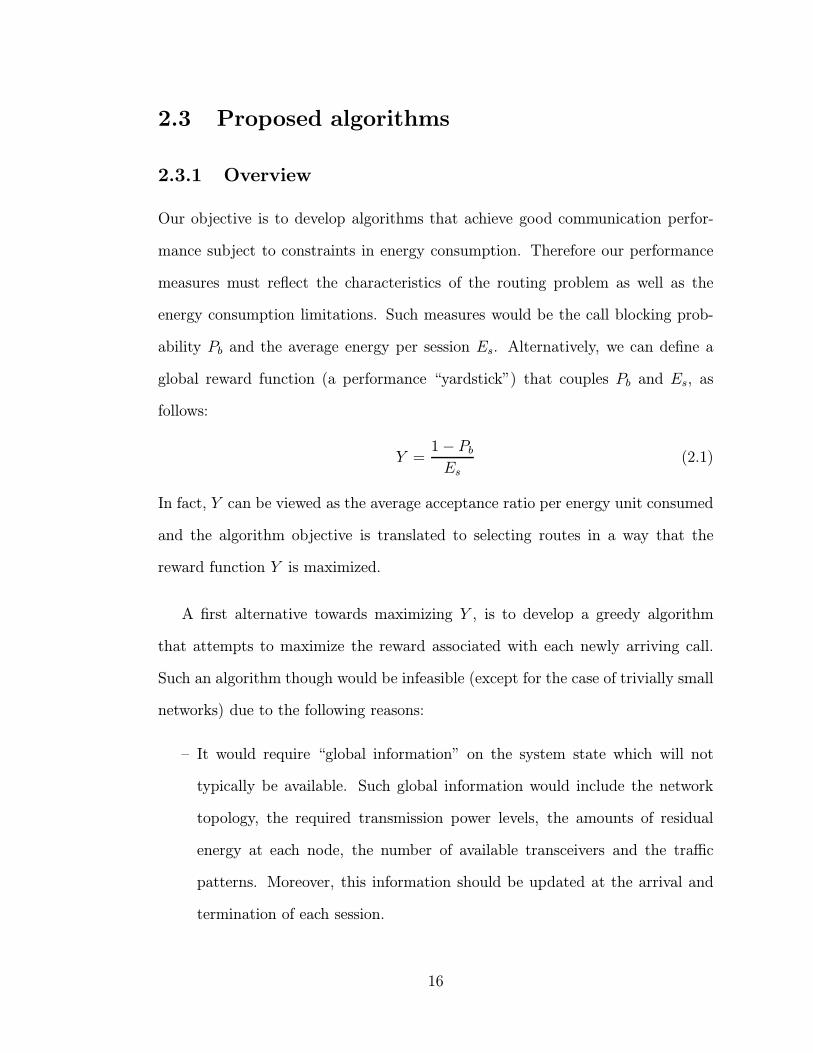
2.3.1 Overview
Our objective is to develop algorithms that achieve good communication perfor-
mance subject to constraints in energy consumption. Therefore our performance
measures must reflect the characteristics of the routing problem as well as the
energy consumption limitations. Such measures would be the call blocking prob-
ability Pb and the average energy per session Es. Alternatively, we can define a
global reward function (a performance “yardstick”) that couples Pb and Es, as
follows:
Y =1− PbEs
(2.1)
In fact, Y can be viewed as the average acceptance ratio per energy unit consumed
and the algorithm objective is translated to selecting routes in a way that the
reward function Y is maximized.
A first alternative towards maximizing Y , is to develop a greedy algorithm
that attempts to maximize the reward associated with each newly arriving call.
Such an algorithm though would be infeasible (except for the case of trivially small
networks) due to the following reasons:
– It would require “global information” on the system state which will not
typically be available. Such global information would include the network
topology, the required transmission power levels, the amounts of residual
energy at each node, the number of available transceivers and the traffic
patterns. Moreover, this information should be updated at the arrival and
termination of each session.
16
– Even if we assumed that we had a centralized mechanism that could collect
“global information”, the greedy maximization approach would have to per-
form an exhaustive search of all possible paths (given the current network
state) if the true optimal solution was to be found. Such an exhaustive search
is infeasible unless we consider trivially small topologies.
The second alternative is to concentrate our efforts on developing distributed
heuristics that rely only on local information to select a route. Each link (i, j) is
associated with a distance metric that indicates the cost of using that link and
may incorporate local information of the transmission power, the residual energy
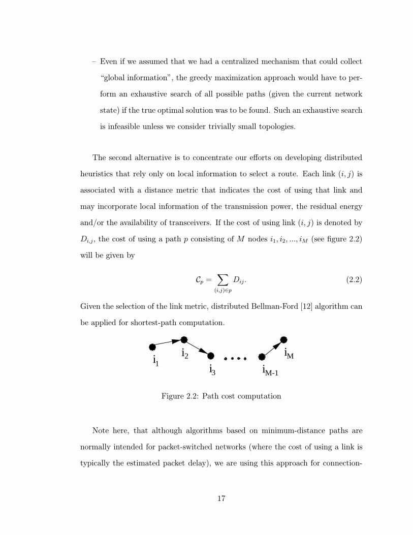
and/or the availability of transceivers. If the cost of using link (i, j) is denoted by
Di,j, the cost of using a path p consisting of M nodes i1, i2, ..., iM (see figure 2.2)
will be given by
Cp =∑
(i,j)∈p
Dij . (2.2)
Given the selection of the link metric, distributed Bellman-Ford [12] algorithm can
be applied for shortest-path computation.
����
����
����
����
���
���
��������������������������������i
ii i
i1
2
3 M-1
M
Figure 2.2: Path cost computation
Note here, that although algorithms based on minimum-distance paths are
normally intended for packet-switched networks (where the cost of using a link is
typically the estimated packet delay), we are using this approach for connection-
17

oriented traffic, by defining a cost for each link that involves various local param-
eters. In telephony networks such a metric is hard to define since energy is not
a concern and delay is not an appropriate metric. Therefore, in the telephone
network the overall objective (blocking probability) cannot be directly mapped to
individual link metrics.
It is very difficult to predict a priori which link metric will result in better
performance. This can only be done by extensive simulation comparison. In the
subsequent sections we define a set of candidate link metrics and compare them
via simulation.
2.3.2 Link metrics
A call request is rejected only if no path exists between source and destination with
available transceivers at each node. Note that if the number of transceivers per
node was large enough, so that availability was always guaranteed (ie no blocking
at all), the problem of minimum energy routing would reduce to determining the
minimum total power path and all calls would be admitted and completed with
minimum energy expenditures 2. When the nodal capacity is finite (as it is in
our case) some nodes have temporarily no transceivers available and they cannot
route or place any new calls. Since the minimum power path will not always be
available, we can search for the lowest total power path in the subgraph defined
by the nodes with nonzero residual capacity and energy and their corresponding
links. In all the proposed metrics, a link that consists of at least one node with
zero residual capacity or residual energy will have an infinite cost.
2provided that all nodes had still some energy reserves
18
(a) Metric M1
Based on the above remarks, we first define link metric M1 which is a direct
measure of the power needed to transmit over a link, provided both nodes have
nonzero residual capacity and energy. Hence the cost of using link (i, j) is defined
by:
D(1)ij =
Pij if Ri, Rj 6= 0 and ERi , E
Rj 6= 0
∞ otherwise(2.3)
where Pij is the power that i needs to transmit to j.
M1 will always provide the minimum power path available, which might not
always be advantageous in terms of overall network performance. A minimum
power path will usually be a multi-hop path as we previously observed and therefore
will occupy more network resources, which could result in blocking of more new
calls. It is also possible, depending on the traffic patterns, that some paths get
heavily utilized and act as bottlenecks (in a static topology the minimum power
path will be the same until any node is blocked), while others consist of lightly
used nodes. Finally, if processing power is not negligible compared to transmitter
power, multi-hop paths could sometimes result in larger energy expenditures.
(b) Metric M2
To address the problem of congested nodes, we define link metric M2 which at-
tempts to discourage use of heavily used paths. Metric M2 is defined by:
D(2)ij =
Pij
min{Ri,Rj}if Ri, Rj 6= 0 and ER
i , ERj 6= 0
∞ otherwise(2.4)
19

M2 favors links that are not heavily utilized by increasing the cost of links that
connect nodes with smaller residual capacity, trying this way to spread the offered
traffic evenly over all paths.
(c) Metric M3
Both M1 and M2 rely on the power level required to successfully transmit to a
one-hop neighbor but ignore an important parameter of the receiving node: its
residual energy. Under certain circumstances, it may be preferable to route a call
over a path that consists of nodes with larger amounts of residual energy, even
though this may result in additional energy consumption by the session. Such a
feature could be used to avoid loading nodes that are low on energy reserves and
we wish to make conservative usage of the remaining energy in order to prolong
their lifetime.
To these ends we propose the use of link metric M3 which is defined by:
D(3)ij =
WpPijPmax
+WeEojERj
if Ri, Rj 6= 0 and ERi , E
Rj 6= 0
∞ otherwise(2.5)
Wp and We are weights that may be adjusted to favor either of the two terms.
Note that in the beginning of network operation the second term is equal for all
nodes (with value 1) and therefore our metric is similar to M1. As the residual
energy of every node begins to drop, the second term will increase and when the
amount of residual energy is low the cost of using the link will become very high.
M3 attempts to introduce some fairness considerations in node usage, so that the
contribution of each node to the aggregate energy consumed by the network is as
even as possible, provided the traffic requirements are uniform.
20
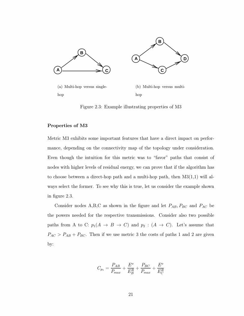
A
B
C
(a) Multi-hop versus single-
hop
A
B
D
C
(b) Multi-hop versus multi-
hop
Figure 2.3: Example illustrating properties of M3
Properties of M3
Metric M3 exhibits some important features that have a direct impact on perfor-
mance, depending on the connectivity map of the topology under consideration.
Even though the intuition for this metric was to “favor” paths that consist of
nodes with higher levels of residual energy, we can prove that if the algorithm has
to choose between a direct-hop path and a multi-hop path, then M3(1,1) will al-
ways select the former. To see why this is true, let us consider the example shown
in figure 2.3.
Consider nodes A,B,C as shown in the figure and let PAB, PBC and PAC be
the powers needed for the respective transmissions. Consider also two possible
paths from A to C: p1(A → B → C) and p2 : (A → C). Let’s assume that
PAC > PAB + PBC . Then if we use metric 3 the costs of paths 1 and 2 are given
by:
Cp1 =PABPmax
+Eo
ERB
+PBCPmax
+Eo
ERC
21
Cp2 =PACPmax
+Eo
ERC
To compare the path costs:
DC = Cp2 − Cp1 =PAC − (PAB + PBC)
Pmax−Eo
ERB
But
0 ≤PAC − (PAB + PBC)
Pmax≤ 1
and
1 ≤Eo
ERB
<∞
Therefore
DC = Cp2 − Cp1 < 0→ Cp2 < Cp1
The above example can be easily generalized in the case when the comparison is
between a path with a direct link versus a path with M links where M ∈ [2, N−1].
Proposition: Let p1 denote a multiple hop path from A to B (p1 : (A → X1 →
X2 → · · · → XN−1 → B) and p2 a direct path (single link) from A to B (p2 : (A→
B)) and let PAB > PAX1 +∑N−2
i=1 PXiXi+1 + PXN−1B. If the link cost is given by
metric M3(1,1) (equation 2.5) then Cp1 > Cp2 will always hold.
Proof: Applying the definitions we have:
Cp1 =PAX1 +
∑i=N−2i=1 PXiXi+1 + PXN−1B
Pmax+ Eo(
N−1∑i=1
1
ERi
+1
ERB
)
22

Cp2 =PABPmax
+Eo
ERB
To compare the path costs:
DC = Cp2 − Cp1 =PAB − (PAX1 +
∑i=N−2i=1 PXiXi+1 + PXN−1B)
Pmax−
N−1∑i=1
Eo
ERi
But
0 ≤PAB − (PAX1 +
∑i=N−2i=1 PXiXi+1 + PXN−1B)
Pmax≤ 1
and
N ≤N−1∑i=1
Eo
ERi
<∞
Therefore
DC = Cp2 − Cp1 < 0→ Cp2 < Cp1
Q.E.D.
Despite this limitation, M3 is very appropriate in situations when the com-
parison is between multiple multi-hop paths. In that case the above proposition
does not apply and the factor which has a large impact on the decision in the
residual energy of the relay nodes. To illustrate this better, consider for exam-
ple the case of two multi-hop paths p1 and p2 as shown in figure 2.3, where both
paths have the same number of hops (2-hops). Hence let p1 : (A → B → D)
and p2 : (A → C → D). Here the critical parameter is the residual energy of
23
the intermediate node of each path and of course the difference in the sum of the
transmission powers of each path.
DC = Cp2 − Cp1 =(PAC + PCD)− (PAB + PBD)
Pmax+ (
Eo
ERC
−Eo
ERB
)
Even though the first term of the above equation will be ∈ [−2, 2] we cannot
determine for sure whether DC will be positive or negative unless we know the
values of ERB and ER
C .
2.4 Simulation model
We have evaluated the performance of the proposed algorithms for a variety of
network parameters such as network size, node density, traffic load, transmission
power level and initial energy resources. We consider random network topologies,
by generating each node’s location randomly within a square region of size 100×100
units. We assume that the existence of a link between any two nodes depends solely
on their Euclidean distance and the propagation loss exponent is taken α = 2.
All links are full-duplex and error-free and without loss of generality, let a node
transmitting at a power level of Po = 0.1 be received by all nodes located within
distance d ≤ do = 10 units. Using this value as a reference, we may compute the
transmission range dmax corresponding to a given Pmax by,
Pmax
Po= (
dmax
do)2 (2.6)
For example if we want a node’s transmission range not to exceed 30 units, its
maximum transmission power level must not exceed Pmax = 0.9.
24
In order to model both sparse and dense topologies, we present results for
networks of N = 10, 20 and 50 nodes and for transmission range values (dmax)
between 30 and 70 units, which as we will show have a direct effect on the resulting
average node degree and the connectivity of the network.
For every network size, we generate 100 random topologies. Note that we
are only interested in connected topologies (performance of a partitioned network
in which not all nodes may communicate with each other was not considered).
Each simulation runs until 20000 call requests have been scheduled, which was
determined to be a sufficient amount of offered load in all the experiments, so that
transient effects can be neglected.
All nodes have equal amounts of initial energy Eo and unless otherwise specified
this energy level is sufficient for the duration of the simulation. We assume initially
that energy is only consumed during transmission and for the whole duration of
a session. For example, a session from node i to node k via node j that lasts for
t time units would consume E = (Pij + Pjk) × t units of energy. The effects of
receive and processing power are incorporated in a separate section. Finally each
node is assumed to have a total of five transceivers (C = 5).
We have assumed in all the simulations that calls arrive independently at each
node following a Poisson distribution with average rate λ such that 0 ≤ λ ≤ 1.
Average session durations are exponentially distributed with µ = 1. For every new
call arrival, the destination is uniformly selected among the remaining nodes.
Performance is measured by the blocking probability Pb, the average energy per
session Es and the performance yardstick Y that we defined in equation 2.1. In
some of the experiments we were also interested in additional performance metrics,
25
such as the the average lifetime of the nodes and the network or the average number
of links per path.
A discrete-event simulation tool has been developed in ANSI C for the pur-
pose of performance measurements. An overview of the model structure and a
description of the main routines and components is provided in the appendix.
2.5 Performance results
2.5.1 Blocking probability (Pb)
In this section we examine the algorithm performance in terms of blocking probabil-
ity versus network parameters, such as the average call arrival rate, the maximum
transmission power, the network size and the node density. We compare M1, M2
and two different cases of M3; one which accounts only for the residual energy of
the receiver (Wp = 0,We = 1) and one that equally considers transmission power
and residual energy (Wp = 1,We = 1).
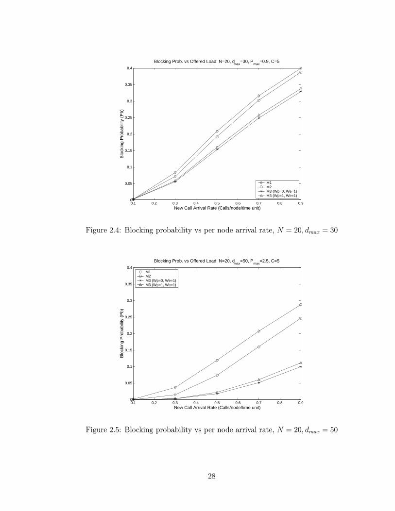
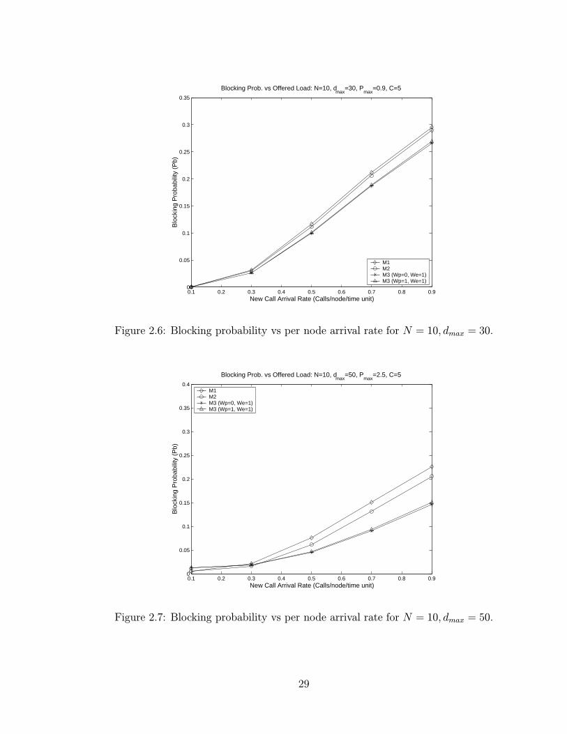
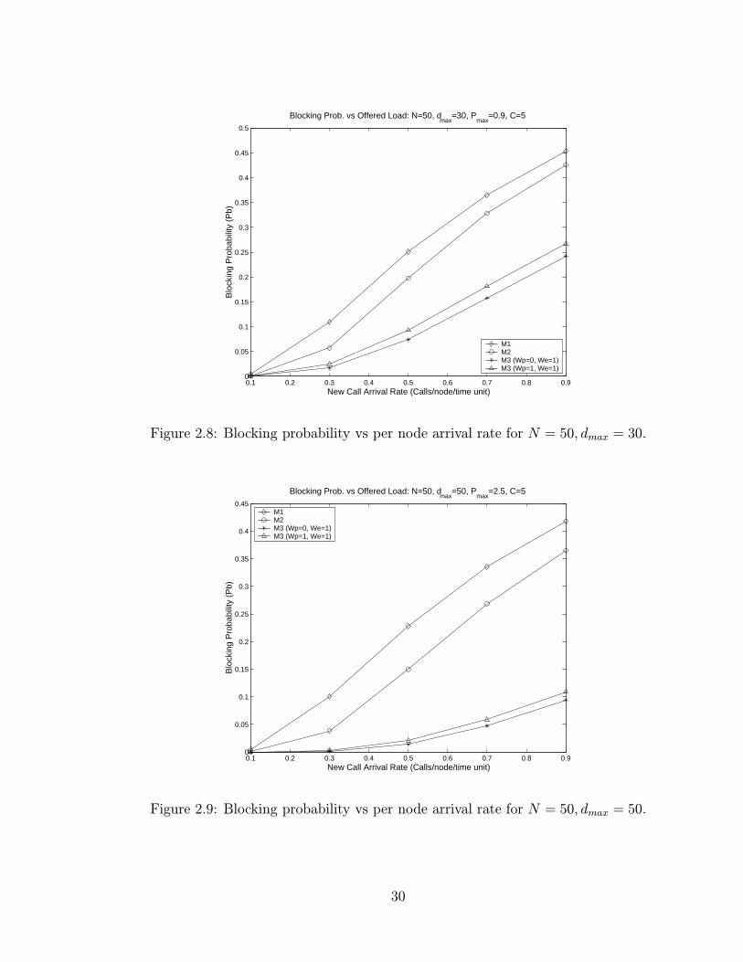
Figures 2.4 and 2.5 illustrate graphically the blocking probability Pb as a func-
tion of the offered load per node, for N = 20 and the cases of dmax = 30 and 50
respectively. The curves plotted in these graphs lead to the following observations:
– In all cases Pb increases as the offered load increases.
– In both graphs M1 exhibits the worst performance among all metrics. The
reason is that M1 always searches for the lowest total power path available,
which is usually a path with a larger number of hops, and therefore it results
in utilization/reservation of larger number of transceivers.
26
– Use of M1 results also in heavier utilization of some paths while at the same
time others may consist of idle nodes. M2 partially solves this problem
and the improvement in Pb is larger especially for the case of larger dmax =
50 (figure 2.5) since increased connectivity provides additional paths and
incoming traffic can be spread over the network more effectively.
– M3 achieves much lower Pb, especially when the transmission range increases,
mainly because of the inherent property of M3 to favor a direct link from
source to destination (if such a link exists which is often the case for high
dmax), but also because of the property to spread the traffic more evenly
among paths in order to balance energy expenditures among all nodes. How-
ever, this comes at the cost of higher amounts of energy expenditures as we
will see in subsequent results.
Similar conclusions, as far as the relative performance comparison of our metrics
is concerned, can be drawn from figures 2.6, 2.7, 2.8 and 2.9, which depict blocking
probability versus offered traffic for networks with N = 10 and N = 50 nodes.
To verify our intuition that M1 and M2 provide on average paths with larger
number of hops, we computed the average number of hops per accepted session
for the above simulations. Our results are summarized in table 2.1 for the cases of
λ = 0.1 and 0.5. Each cell in the table consists of the average number of hops per
session and the corresponding standard deviation. These results clearly indicate
that M1 and M2 tend to utilize paths with larger number of hops.
27
0.1 0.2 0.3 0.4 0.5 0.6 0.7 0.8 0.90
0.05
0.1
0.15
0.2
0.25
0.3
0.35
0.4
Blocking Prob. vs Offered Load: N=20, dmax
=30, Pmax
=0.9, C=5
Blo
ckin
g P
roba
bilit
y (P
b)
New Call Arrival Rate (Calls/node/time unit)
M1 M2 M3 (Wp=0, We=1)M3 (Wp=1, We=1)
Figure 2.4: Blocking probability vs per node arrival rate, N = 20, dmax = 30
0.1 0.2 0.3 0.4 0.5 0.6 0.7 0.8 0.90
0.05
0.1
0.15
0.2
0.25
0.3
0.35
0.4
Blocking Prob. vs Offered Load: N=20, dmax
=50, Pmax
=2.5, C=5
Blo
ckin
g P
roba
bilit
y (P
b)
New Call Arrival Rate (Calls/node/time unit)
M1 M2 M3 (Wp=0, We=1)M3 (Wp=1, We=1)
Figure 2.5: Blocking probability vs per node arrival rate, N = 20, dmax = 50
28
0.1 0.2 0.3 0.4 0.5 0.6 0.7 0.8 0.90
0.05
0.1
0.15
0.2
0.25
0.3
0.35
Blocking Prob. vs Offered Load: N=10, dmax
=30, Pmax
=0.9, C=5
Blo
ckin
g P
roba
bilit
y (P
b)
New Call Arrival Rate (Calls/node/time unit)
M1 M2 M3 (Wp=0, We=1)M3 (Wp=1, We=1)
Figure 2.6: Blocking probability vs per node arrival rate for N = 10, dmax = 30.
0.1 0.2 0.3 0.4 0.5 0.6 0.7 0.8 0.90
0.05
0.1
0.15
0.2
0.25
0.3
0.35
0.4
Blocking Prob. vs Offered Load: N=10, dmax
=50, Pmax
=2.5, C=5
Blo
ckin
g P
roba
bilit
y (P
b)
New Call Arrival Rate (Calls/node/time unit)
M1 M2 M3 (Wp=0, We=1)M3 (Wp=1, We=1)
Figure 2.7: Blocking probability vs per node arrival rate for N = 10, dmax = 50.
29
0.1 0.2 0.3 0.4 0.5 0.6 0.7 0.8 0.90
0.05
0.1
0.15
0.2
0.25
0.3
0.35
0.4
0.45
0.5
Blocking Prob. vs Offered Load: N=50, dmax
=30, Pmax
=0.9, C=5
Blo
ckin
g P
roba
bilit
y (P
b)
New Call Arrival Rate (Calls/node/time unit)
M1 M2 M3 (Wp=0, We=1)M3 (Wp=1, We=1)
Figure 2.8: Blocking probability vs per node arrival rate for N = 50, dmax = 30.
0.1 0.2 0.3 0.4 0.5 0.6 0.7 0.8 0.90
0.05
0.1
0.15
0.2
0.25
0.3
0.35
0.4
0.45
Blocking Prob. vs Offered Load: N=50, dmax
=50, Pmax
=2.5, C=5
Blo
ckin
g P
roba
bilit
y (P
b)
New Call Arrival Rate (Calls/node/time unit)
M1 M2 M3 (Wp=0, We=1)M3 (Wp=1, We=1)
Figure 2.9: Blocking probability vs per node arrival rate for N = 50, dmax = 50.
30
λ = 0.1 λ = 0.5
Metric dmax = 30 dmax = 50 dmax = 30 dmax = 50
M1 4.06 ; 0.59 3.89 ; 0.44 3.62 ; 0.44 3.51 ; 0.36
M2 4.10 ; 0.58 3.98 ; 0.41 3.62 ; 0.42 3.46 ; 0.31
M3(0,1) 2.87 ; 0.38 2.79 ; 0.30 1.59 ; 0.14 1.59 ; 0.14
M3(1,1) 2.87 ; 0.38 2.80 ; 0.30 1.60 ; 0.14 1.60 ; 0.14
Table 2.1: Average number of hops and standard deviation per admitted session
for N = 20
2.5.2 Average energy per session (Es)
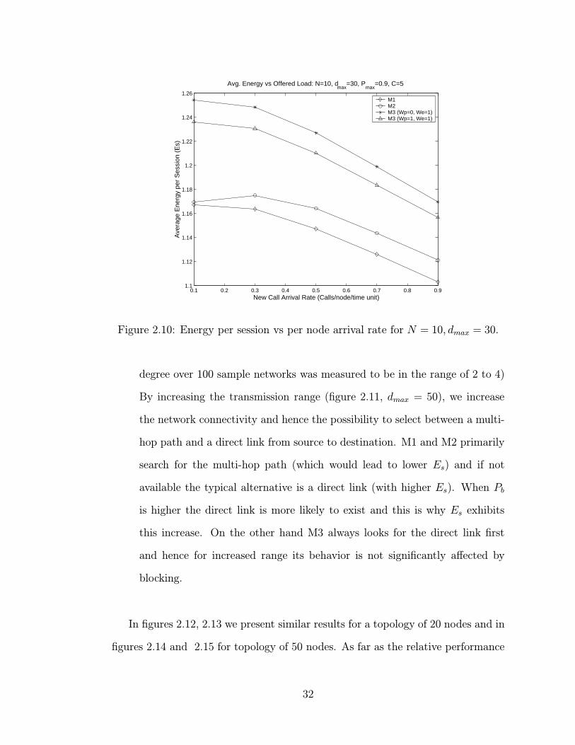
Figures 2.10 and 2.11 depict the average energy per accepted session (Es) versus
the arrival rate λ, again for N = 20 and the cases of dmax = 30 and dmax = 50.
We can draw the following remarks from these plots:
– M1 and M2 result in lower energy consumption, since by definition they
admit sessions in the lowest transmission power path available. Nonetheless,
this comes at the cost of higher Pb as we pointed out in the previous section.
The inherent trade-off between Pb and Es is rather clear from these results
and is evaluated separately by examining the behavior of the yardstick Y .
– For the case of lower dmax (figure 2.10) we observe that Es starts exhibiting
some decrease with higher values of λ. The reason for such a behavior is that
when traffic load (and therefore blocking) is high, calls that require fewer hops
from source to destination (ie fewer node resources) have a higher chance of
being admitted. For N = 10 (sparse topologies) and for low transmission
range we do not have significant route redundancy (in fact, the average node
31
0.1 0.2 0.3 0.4 0.5 0.6 0.7 0.8 0.91.1
1.12
1.14
1.16
1.18
1.2
1.22
1.24
1.26
Avg. Energy vs Offered Load: N=10, dmax
=30, Pmax
=0.9, C=5
New Call Arrival Rate (Calls/node/time unit)
Ave
rage
Ene
rgy
per
Ses
sion
(E
s)
M1 M2 M3 (Wp=0, We=1)M3 (Wp=1, We=1)
Figure 2.10: Energy per session vs per node arrival rate for N = 10, dmax = 30.
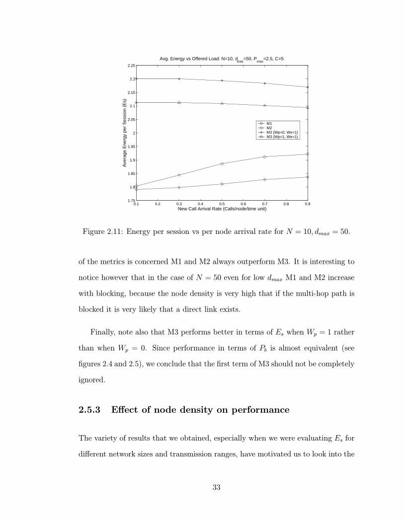
degree over 100 sample networks was measured to be in the range of 2 to 4)
By increasing the transmission range (figure 2.11, dmax = 50), we increase
the network connectivity and hence the possibility to select between a multi-
hop path and a direct link from source to destination. M1 and M2 primarily
search for the multi-hop path (which would lead to lower Es) and if not
available the typical alternative is a direct link (with higher Es). When Pb
is higher the direct link is more likely to exist and this is why Es exhibits
this increase. On the other hand M3 always looks for the direct link first
and hence for increased range its behavior is not significantly affected by
blocking.
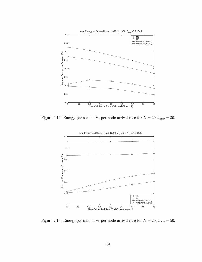
In figures 2.12, 2.13 we present similar results for a topology of 20 nodes and in
figures 2.14 and 2.15 for topology of 50 nodes. As far as the relative performance
32
0.1 0.2 0.3 0.4 0.5 0.6 0.7 0.8 0.91.75
1.8
1.85
1.9
1.95
2
2.05
2.1
2.15
2.2
2.25
Avg. Energy vs Offered Load: N=10, dmax
=50, Pmax
=2.5, C=5
New Call Arrival Rate (Calls/node/time unit)
Ave
rage
Ene
rgy
per
Ses
sion
(E
s)M1 M2 M3 (Wp=0, We=1)M3 (Wp=1, We=1)
Figure 2.11: Energy per session vs per node arrival rate for N = 10, dmax = 50.
of the metrics is concerned M1 and M2 always outperform M3. It is interesting to
notice however that in the case of N = 50 even for low dmax M1 and M2 increase
with blocking, because the node density is very high that if the multi-hop path is
blocked it is very likely that a direct link exists.
Finally, note also that M3 performs better in terms of Es when Wp = 1 rather
than when Wp = 0. Since performance in terms of Pb is almost equivalent (see
figures 2.4 and 2.5), we conclude that the first term of M3 should not be completely
ignored.
2.5.3 Effect of node density on performance
The variety of results that we obtained, especially when we were evaluating Es for
different network sizes and transmission ranges, have motivated us to look into the
33
0.1 0.2 0.3 0.4 0.5 0.6 0.7 0.8 0.91.2
1.25
1.3
1.35
1.4
1.45
1.5
1.55
1.6
Avg. Energy vs Offered Load: N=20, dmax
=30, Pmax
=0.9, C=5
New Call Arrival Rate (Calls/node/time unit)
Ave
rage
Ene
rgy
per
Ses
sion
(E
s)
M1 M2 M3 (Wp=0, We=1)M3 (Wp=1, We=1)
Figure 2.12: Energy per session vs per node arrival rate for N = 20, dmax = 30.
0.1 0.2 0.3 0.4 0.5 0.6 0.7 0.8 0.91
1.2
1.4
1.6
1.8
2
2.2
Avg. Energy vs Offered Load: N=20, dmax
=50, Pmax
=2.5, C=5
New Call Arrival Rate (Calls/node/time unit)
Ave
rage
Ene
rgy
per
Ses
sion
(E
s)
M1 M2 M3 (Wp=0, We=1)M3 (Wp=1, We=1)
Figure 2.13: Energy per session vs per node arrival rate for N = 20, dmax = 50.
34

0.1 0.2 0.3 0.4 0.5 0.6 0.7 0.8 0.90.8
0.9
1
1.1
1.2
1.3
1.4
1.5
Avg. Energy vs Offered Load: N=50, dmax
=30, Pmax
=0.9, C=5
New Call Arrival Rate (Calls/node/time unit)
Ave
rage
Ene
rgy
per
Ses
sion
(E
s)
M1 M2 M3 (Wp=0, We=1)M3 (Wp=1, We=1)
Figure 2.14: Energy per session vs per node arrival rate for N = 50, dmax = 30.
0.1 0.2 0.3 0.4 0.5 0.6 0.7 0.8 0.90.8
1
1.2
1.4
1.6
1.8
2
2.2
2.4
2.6
Avg. Energy vs Offered Load: N=50, dmax
=50, Pmax
=2.5, C=5
New Call Arrival Rate (Calls/node/time unit)
Ave
rage
Ene
rgy
per
Ses
sion
(E
s)
M1 M2 M3 (Wp=0, We=1)M3 (Wp=1, We=1)
Figure 2.15: Energy per session vs per node arrival rate for N = 50, dmax = 50.
35
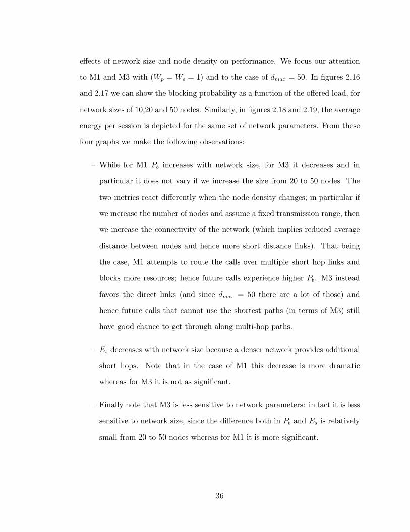
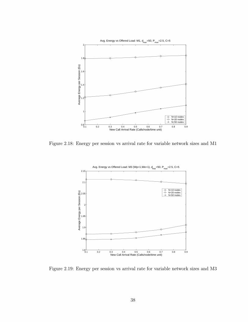
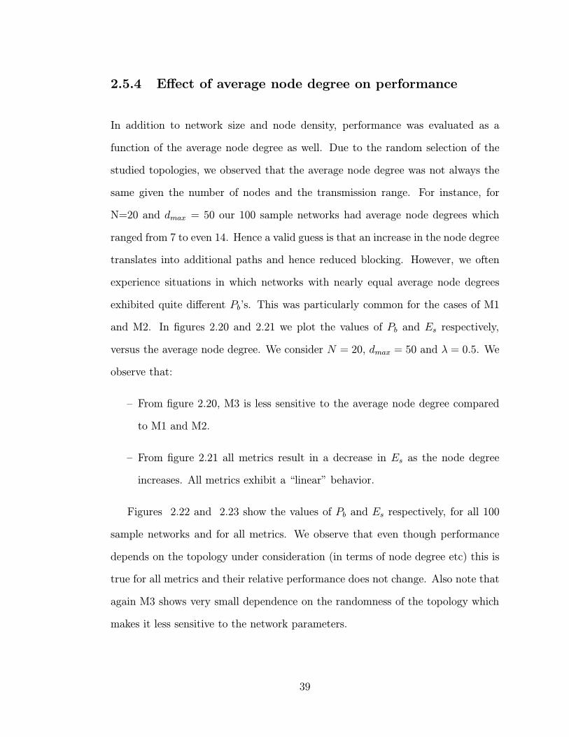
effects of network size and node density on performance. We focus our attention
to M1 and M3 with (Wp = We = 1) and to the case of dmax = 50. In figures 2.16
and 2.17 we can show the blocking probability as a function of the offered load, for
network sizes of 10,20 and 50 nodes. Similarly, in figures 2.18 and 2.19, the average
energy per session is depicted for the same set of network parameters. From these
four graphs we make the following observations:
– While for M1 Pb increases with network size, for M3 it decreases and in
particular it does not vary if we increase the size from 20 to 50 nodes. The
two metrics react differently when the node density changes; in particular if
we increase the number of nodes and assume a fixed transmission range, then
we increase the connectivity of the network (which implies reduced average
distance between nodes and hence more short distance links). That being
the case, M1 attempts to route the calls over multiple short hop links and
blocks more resources; hence future calls experience higher Pb. M3 instead
favors the direct links (and since dmax = 50 there are a lot of those) and
hence future calls that cannot use the shortest paths (in terms of M3) still
have good chance to get through along multi-hop paths.
– Es decreases with network size because a denser network provides additional
short hops. Note that in the case of M1 this decrease is more dramatic
whereas for M3 it is not as significant.
– Finally note that M3 is less sensitive to network parameters: in fact it is less
sensitive to network size, since the difference both in Pb and Es is relatively
small from 20 to 50 nodes whereas for M1 it is more significant.
36

0.1 0.2 0.3 0.4 0.5 0.6 0.7 0.8 0.90
0.05
0.1
0.15
0.2
0.25
0.3
0.35
0.4
0.45
Blocking Prob. vs Offered Load: M1, dmax
=50, Pmax
=2.5, C=5
New Call Arrival Rate (Calls/node/time unit)
Blo
ckin
g P
roba
bilit
y (P
b)
N=10 nodesN=20 nodesN=50 nodes
Figure 2.16: Blocking probability vs arrival rate for variable network sizes and M1
0.1 0.2 0.3 0.4 0.5 0.6 0.7 0.8 0.90
0.02
0.04
0.06
0.08
0.1
0.12
0.14
0.16
Blocking Prob. vs Offered Load: M3 (Wp=1,We=1), dmax
=50, Pmax
=2.5, C=5
New Call Arrival Rate (Calls/node/time unit)
Blo
ckin
g P
roba
bilit
y (P
b)
N=10 nodesN=20 nodesN=50 nodes
Figure 2.17: Blocking probability vs arrival rate for variable network sizes and M3
37
0.1 0.2 0.3 0.4 0.5 0.6 0.7 0.8 0.90.8
1
1.2
1.4
1.6
1.8
2
Avg. Energy vs Offered Load: M1, dmax
=50, Pmax
=2.5, C=5
New Call Arrival Rate (Calls/node/time unit)
Ave
rage
Ene
rgy
per
Ses
sion
(E
s)
N=10 nodesN=20 nodesN=50 nodes
Figure 2.18: Energy per session vs arrival rate for variable network sizes and M1
0.1 0.2 0.3 0.4 0.5 0.6 0.7 0.8 0.91.8
1.85
1.9
1.95
2
2.05
2.1
2.15
Avg. Energy vs Offered Load: M3 (Wp=1,We=1), dmax
=50, Pmax
=2.5, C=5
New Call Arrival Rate (Calls/node/time unit)
Ave
rage
Ene
rgy
per
Ses
sion
(E
s)
N=10 nodesN=20 nodesN=50 nodes
Figure 2.19: Energy per session vs arrival rate for variable network sizes and M3
38
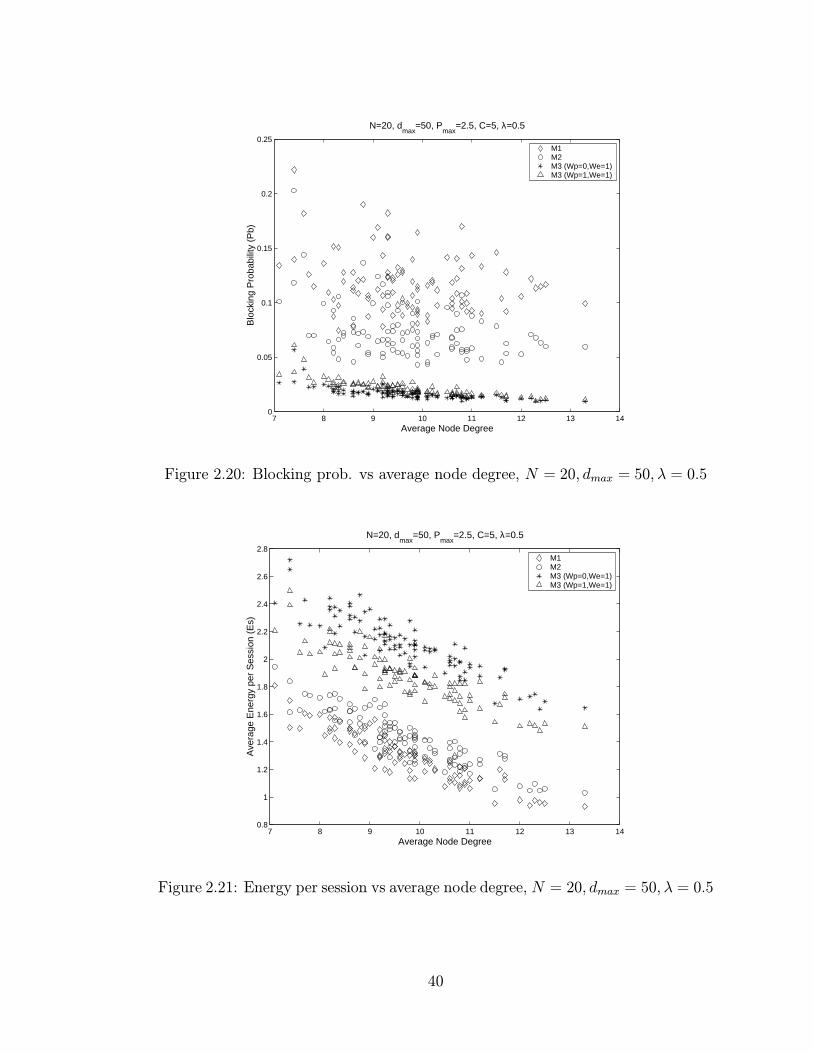
2.5.4 Effect of average node degree on performance
In addition to network size and node density, performance was evaluated as a
function of the average node degree as well. Due to the random selection of the
studied topologies, we observed that the average node degree was not always the
same given the number of nodes and the transmission range. For instance, for
N=20 and dmax = 50 our 100 sample networks had average node degrees which
ranged from 7 to even 14. Hence a valid guess is that an increase in the node degree
translates into additional paths and hence reduced blocking. However, we often
experience situations in which networks with nearly equal average node degrees
exhibited quite different Pb’s. This was particularly common for the cases of M1
and M2. In figures 2.20 and 2.21 we plot the values of Pb and Es respectively,
versus the average node degree. We consider N = 20, dmax = 50 and λ = 0.5. We
observe that:
– From figure 2.20, M3 is less sensitive to the average node degree compared
to M1 and M2.
– From figure 2.21 all metrics result in a decrease in Es as the node degree
increases. All metrics exhibit a “linear” behavior.
Figures 2.22 and 2.23 show the values of Pb and Es respectively, for all 100
sample networks and for all metrics. We observe that even though performance
depends on the topology under consideration (in terms of node degree etc) this is
true for all metrics and their relative performance does not change. Also note that
again M3 shows very small dependence on the randomness of the topology which
makes it less sensitive to the network parameters.
39
7 8 9 10 11 12 13 140
0.05
0.1
0.15
0.2
0.25
Average Node Degree
Blo
ckin
g P
roba
bilit
y (P
b)
N=20, dmax
=50, Pmax
=2.5, C=5, λ=0.5
M1 M2 M3 (Wp=0,We=1)M3 (Wp=1,We=1)
Figure 2.20: Blocking prob. vs average node degree, N = 20, dmax = 50, λ = 0.5
7 8 9 10 11 12 13 140.8
1
1.2
1.4
1.6
1.8
2
2.2
2.4
2.6
2.8
Average Node Degree
Ave
rage
Ene
rgy
per
Ses
sion
(E
s)
N=20, dmax
=50, Pmax
=2.5, C=5, λ=0.5
M1 M2 M3 (Wp=0,We=1)M3 (Wp=1,We=1)
Figure 2.21: Energy per session vs average node degree, N = 20, dmax = 50, λ = 0.5
40
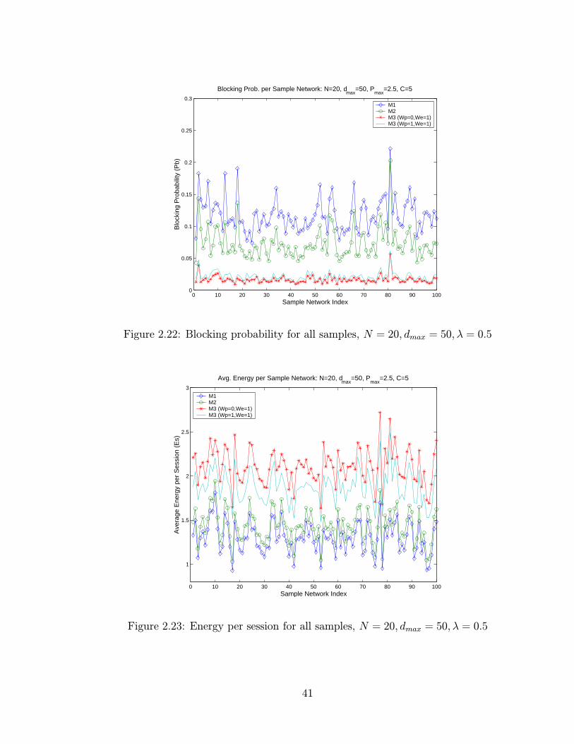
0 10 20 30 40 50 60 70 80 90 1000
0.05
0.1
0.15
0.2
0.25
0.3
Sample Network Index
Blo
ckin
g P
roba
bilit
y (P
b)
Blocking Prob. per Sample Network: N=20, dmax
=50, Pmax
=2.5, C=5
M1 M2 M3 (Wp=0,We=1)M3 (Wp=1,We=1)
Figure 2.22: Blocking probability for all samples, N = 20, dmax = 50, λ = 0.5
0 10 20 30 40 50 60 70 80 90 100
1
1.5
2
2.5
3
Sample Network Index
Ave
rage
Ene
rgy
per
Ses
sion
(E
s)
Avg. Energy per Sample Network: N=20, dmax
=50, Pmax
=2.5, C=5
M1 M2 M3 (Wp=0,We=1)M3 (Wp=1,We=1)
Figure 2.23: Energy per session for all samples, N = 20, dmax = 50, λ = 0.5
41
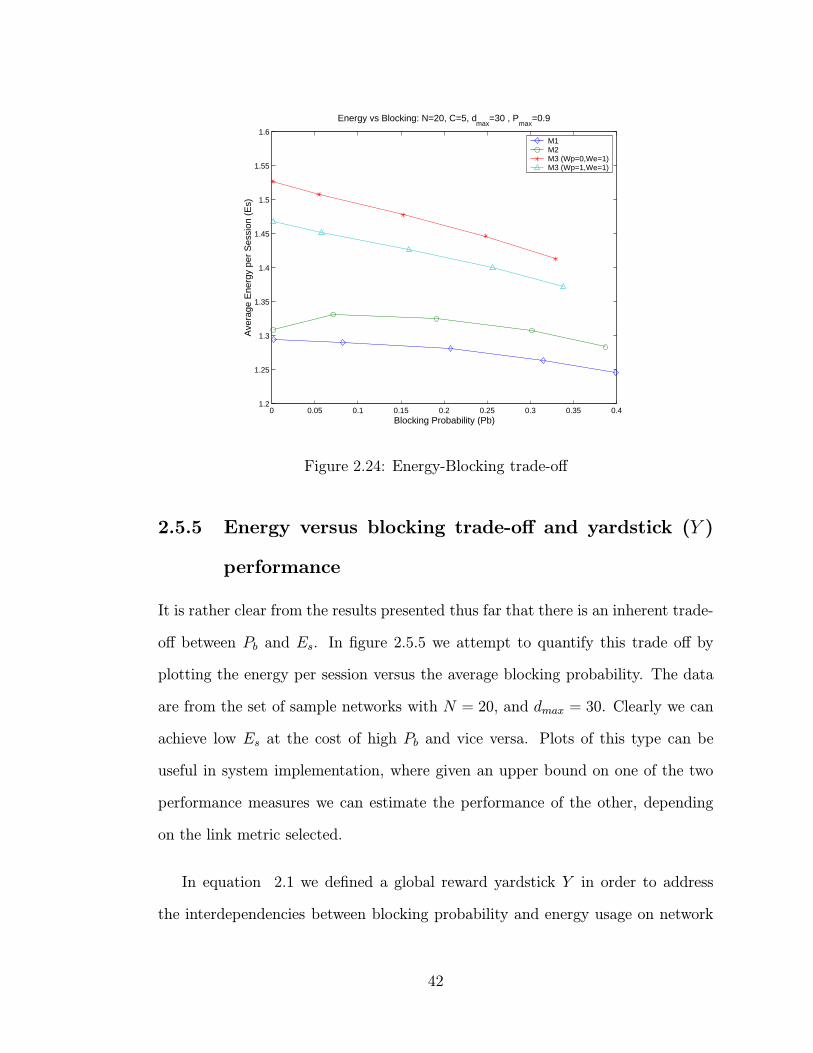
0 0.05 0.1 0.15 0.2 0.25 0.3 0.35 0.41.2
1.25
1.3
1.35
1.4
1.45
1.5
1.55
1.6
Blocking Probability (Pb)
Ave
rage
Ene
rgy
per
Ses
sion
(E
s)
Energy vs Blocking: N=20, C=5, dmax
=30 , Pmax
=0.9
M1 M2 M3 (Wp=0,We=1)M3 (Wp=1,We=1)
Figure 2.24: Energy-Blocking trade-off
2.5.5 Energy versus blocking trade-off and yardstick (Y )
performance
It is rather clear from the results presented thus far that there is an inherent trade-
off between Pb and Es. In figure 2.5.5 we attempt to quantify this trade off by
plotting the energy per session versus the average blocking probability. The data
are from the set of sample networks with N = 20, and dmax = 30. Clearly we can
achieve low Es at the cost of high Pb and vice versa. Plots of this type can be
useful in system implementation, where given an upper bound on one of the two
performance measures we can estimate the performance of the other, depending
on the link metric selected.
In equation 2.1 we defined a global reward yardstick Y in order to address
the interdependencies between blocking probability and energy usage on network
42
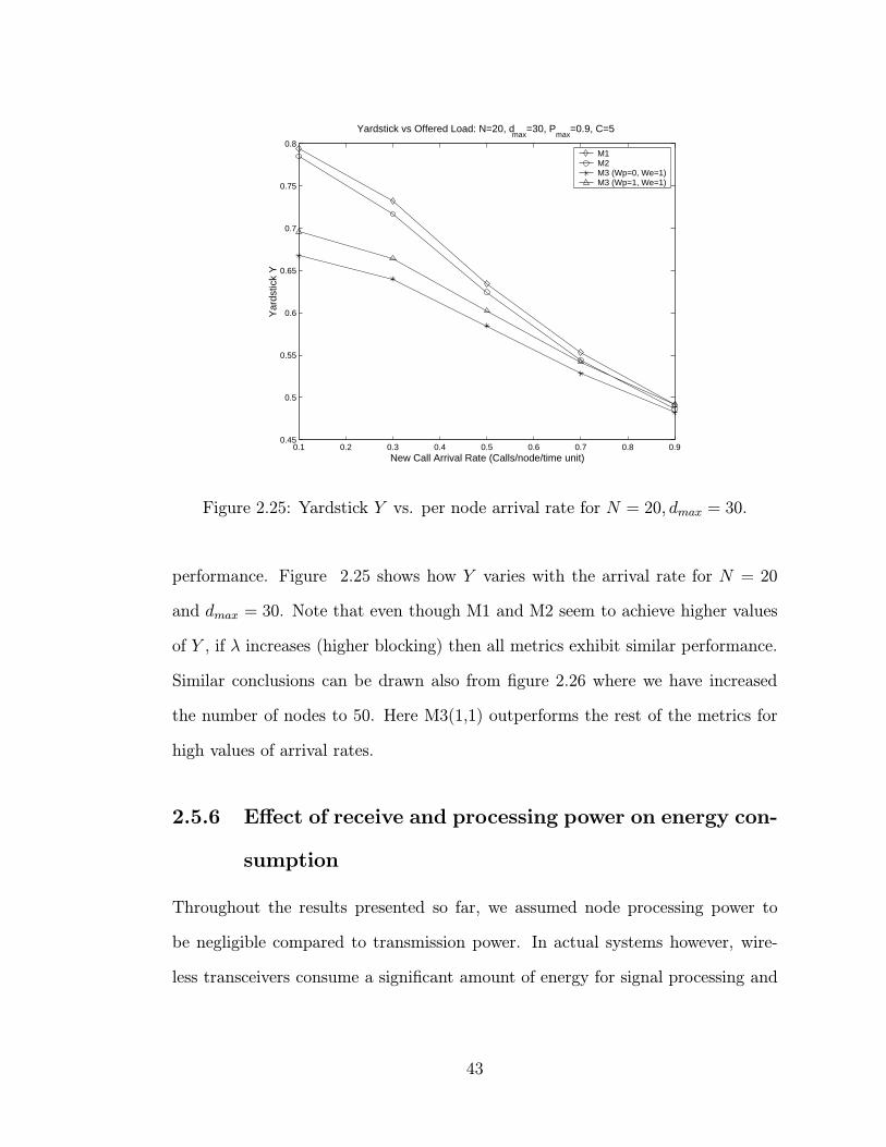
0.1 0.2 0.3 0.4 0.5 0.6 0.7 0.8 0.90.45
0.5
0.55
0.6
0.65
0.7
0.75
0.8
Yardstick vs Offered Load: N=20, dmax
=30, Pmax
=0.9, C=5
New Call Arrival Rate (Calls/node/time unit)
Yar
dstic
k Y
M1 M2 M3 (Wp=0, We=1)M3 (Wp=1, We=1)
Figure 2.25: Yardstick Y vs. per node arrival rate for N = 20, dmax = 30.
performance. Figure 2.25 shows how Y varies with the arrival rate for N = 20
and dmax = 30. Note that even though M1 and M2 seem to achieve higher values
of Y , if λ increases (higher blocking) then all metrics exhibit similar performance.
Similar conclusions can be drawn also from figure 2.26 where we have increased
the number of nodes to 50. Here M3(1,1) outperforms the rest of the metrics for
high values of arrival rates.
2.5.6 Effect of receive and processing power on energy con-
sumption
Throughout the results presented so far, we assumed node processing power to
be negligible compared to transmission power. In actual systems however, wire-
less transceivers consume a significant amount of energy for signal processing and
43

0.1 0.2 0.3 0.4 0.5 0.6 0.7 0.8 0.90.5
0.6
0.7
0.8
0.9
1
1.1
1.2
1.3
Yardstick vs Offered Load: N=50, dmax
=30, Pmax
=0.9, C=5
Yar
dstic
k Y
New Call Arrival Rate (Calls/node/time unit)
M1 M2 M3 (Wp=0, We=1)M3 (Wp=1, We=1)
Figure 2.26: Yardstick Y vs. per node arrival rate for N = 50, dmax = 30.
other tasks that are critical for performing relaying of sessions. A key feature of
our simulation model enables us to quantify the effects of non-negligible processing
power. Although it is extremely hard to capture the actual energy depletion pat-
tern, we have assumed that each wireless transceiver consumes a constant amount
of power (for processing and receiving), denoted by Pproc, whenever it is being used
to ”serve” an active session. Such an assumption is not unreasonable as in fact
receive and processing power do not depend on distance from the transmitter.
For simulation purposes we consider 100 random topologies with N = 20 nodes
We have pre-calculated the average transmission power for all sample networks in
the case of Pmax = 2.5. The average value of the transmitted power was equal to
P̄tr1.1. Given a fixed arrival rate (λ = 0.5) we ran simulations for all metrics for
different values of processing power. In fact we chose Pproc to be 0, 1%, 10%, 30%
44

0 0.05 0.1 0.15 0.2 0.25 0.3 0.35 0.4 0.45 0.51
1.5
2
2.5
3
3.5
Avg. Energy vs Processing Power: N=20, dmax
=50, Pmax
=2.5, C=5, λ=0.5
Processing Power (% of average transmission power)
Ave
rage
Ene
rgy
per
Ses
sion
(E
s)
M1 M2 M3 (Wp=0, We=1)M3 (Wp=1, We=1)
Figure 2.27: Effect of processing power on Es
and 50% of the average transmission power and nodes consume energy at a rate of
Pproc throughout the duration of the sessions they serve. The results are depicted
in figure 2.5.6. We observe that Es has a higher slope for M1 and M2 rather for
M3. Even though for Pproc ≤ 0.2 × P̄tr M1 and M2 perform better, after Pproc
exceeds 25% of P̄tr M3 starts performing better. This is because M1 and M2 favor
the use of multiple small hops which at the same time involve operation of more
nodes. Clearly these results indicate that the contribution of processing power to
the overall expenditures (and therefore to system performance) should not at all
be neglected.
45
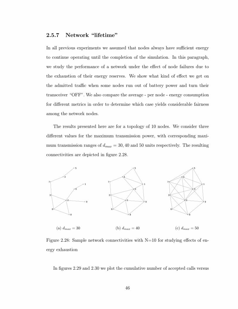
2.5.7 Network “lifetime”
In all previous experiments we assumed that nodes always have sufficient energy
to continue operating until the completion of the simulation. In this paragraph,
we study the performance of a network under the effect of node failures due to
the exhaustion of their energy reserves. We show what kind of effect we get on
the admitted traffic when some nodes run out of battery power and turn their
transceiver “OFF”. We also compare the average - per node - energy consumption
for different metrics in order to determine which case yields considerable fairness
among the network nodes.
The results presented here are for a topology of 10 nodes. We consider three
different values for the maximum transmission power, with corresponding maxi-
mum transmission ranges of dmax = 30, 40 and 50 units respectively. The resulting
connectivities are depicted in figure 2.28.
0
1
2
3
4
5
6
7
8
9
(a) dmax = 30
0
1
2
3
4
5
6
7
8
9
(b) dmax = 40
0
1
2
3
4
5
6
7
8
9
(c) dmax = 50
Figure 2.28: Sample network connectivities with N=10 for studying effects of en-
ergy exhaustion
In figures 2.29 and 2.30 we plot the cumulative number of accepted calls versus
46
the simulation time for the case of the network of figure 2.28(b) and for λ = 0.3
and 0.9 respectively. We compare performance of M1 versus M3 (Wp = 1,We = 1)
and observe the following:
– As nodes begin to switch to OFF state, the rate of accepted calls starts de-
creasing. Therefore, in order to maintain acceptable performance, an algo-
rithm should try to balance the energy consumption evenly among all nodes
so that the time until the first node turns OFF is maximized. Metric M3
achieves that to some significant extent, since the interval from the beginning
of the simulation until the first node turns its power OFF is longer.
– The results are not sensitive to the rate of offered traffic, as far as the rela-
tive performance of the metrics is concerned. Obviously, higher λ results in
shorter network lifetime.
When we increase the maximum transmission range to dmax = 50 (see fig-
ure 2.28(c)), we observe that M3 results in more rapid network partitioning. In
figures 2.31 and 2.32, we plot the cumulative number of accepted calls versus
the simulation time for the case of the network of figure 2.28(c) (dmax = 50 and
for λ = 0.3 and 0.9 respectively). Due to the nature of M1 to “favor” lower
power paths, certain nodes get over-loaded and the time until the first node turns
its power OFF is shorter as compared with M3. However, due to the increased
transmission range, we observe from the connectivity map that there exist a lot of
direct links between nodes which will be “favored” by M3. Even though M3 tries
to maintain a balance among all nodes in terms of energy consumption, most of
its nodes will turn OFF shortly after the first node does so, and the average time
until the network gets partitioned is shorter compared to the case of M1.
47

0 1000 2000 3000 4000 5000 6000 70000
2000
4000
6000
8000
10000
12000
Time t
Agg
rega
te N
umbe
r of
Acc
epte
d C
alls
dmax
=40, Pmax
=1.6, λ = 0.3, C=5
M1
M3 (Wp=W
e=1)
o
o
M1:1st node goes OFF
M3:1st node goes OFF
Figure 2.29: Number of accepted calls vs time; N = 10, dmax = 40 and λ = 0.3
0 500 1000 1500 2000 25000
2000
4000
6000
8000
10000
12000
Time t
Agg
rega
te N
umbe
r of
Acc
epte
d C
alls
dmax
=40, Pmax
=1.6, λ = 0.9, C=5
M1
M3 (Wp=W
e=1)
o
o
M1:1st node goes OFF
M3:1st node goes OFF
Figure 2.30: Number of accepted calls vs time; N = 10, dmax = 40 and λ = 0.9
48
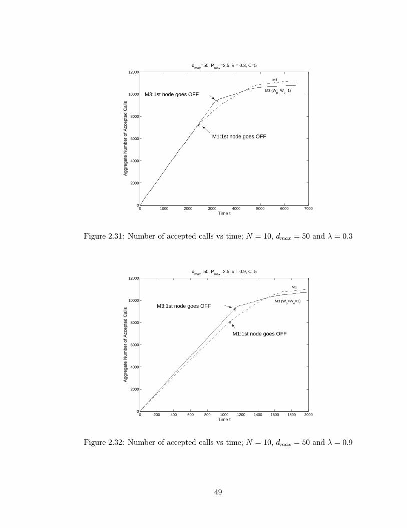
0 1000 2000 3000 4000 5000 6000 70000
2000
4000
6000
8000
10000
12000
Time t
Agg
rega
te N
umbe
r of
Acc
epte
d C
alls
dmax
=50, Pmax
=2.5, λ = 0.3, C=5
M3 (Wp=W
e=1)
M1
o
o
M1:1st node goes OFF
M3:1st node goes OFF
Figure 2.31: Number of accepted calls vs time; N = 10, dmax = 50 and λ = 0.3
0 200 400 600 800 1000 1200 1400 1600 1800 20000
2000
4000
6000
8000
10000
12000
Time t
Agg
rega
te N
umbe
r of
Acc
epte
d C
alls
dmax
=50, Pmax
=2.5, λ = 0.9, C=5
M3 (Wp=W
e=1)
M1
o
o
M1:1st node goes OFF
M3:1st node goes OFF
Figure 2.32: Number of accepted calls vs time; N = 10, dmax = 50 and λ = 0.9
49

To verify our intuition that M3 produces some amount of fairness among
nodes, we ran some experiments for all three connectivity maps of figure 2.28
and examined the energy reserves of all nodes in each case. In particular, let
E = [E0, E1, · · · , EN−1] represent a vector of energy expenditures, with Ei being
the ratio of energy spent versus initial energy for node i. Our simulations termi-
nate before any node runs out of energy and in tables 2.2 and 2.3 we summarize
the statistics of our measurements. Each cell contains four quantities, the mean
value (averaged over all N nodes) the standard deviation, the minimum and the
maximum amounts of energy consumed by any node in the following format:
Mean(E) ; StDev(E)
Min(E) - Max(E)
We make the following observations:
– The average energy per node for the case of M1 does not vary by increasing
the transmission range, whereas this is not the case for M3.
– For M3, Es exhibits smaller standard deviation, which means that the energy
levels are more balanced among all nodes.
2.6 Conclusions
We compared a set of link metrics that can be used for selecting routes in a wire-
less static ad-hoc network where the objective is to minimize blocking probability
subject to energy constraints. We illustrated the trade-offs between blocking and
energy consumption and compared these metrics under different values of the net-
work parameters. Metric M3 combines local information of the transmission power
50
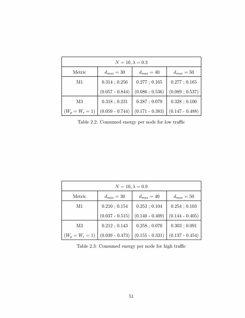
N = 10, λ = 0.3
Metric dmax = 30 dmax = 40 dmax = 50
M1 0.314 ; 0.256 0.277 ; 0.165 0.277 ; 0.165
(0.057 - 0.844) (0.086 ; 0.536) (0.089 ; 0.537)
M3 0.318 ; 0.231 0.287 ; 0.079 0.328 ; 0.100
(Wp = We = 1) (0.059 - 0.744) (0.171 - 0.383) (0.147 - 0.488)
Table 2.2: Consumed energy per node for low traffic
N = 10, λ = 0.9
Metric dmax = 30 dmax = 40 dmax = 50
M1 0.210 ; 0.154 0.253 ; 0.104 0.254 ; 0.103
(0.037 - 0.515) (0.140 - 0.409) (0.144 - 0.405)
M3 0.212 ; 0.143 0.258 ; 0.070 0.303 ; 0.091
(Wp = We = 1) (0.039 - 0.473) (0.155 - 0.331) (0.137 - 0.454)
Table 2.3: Consumed energy per node for high traffic
51
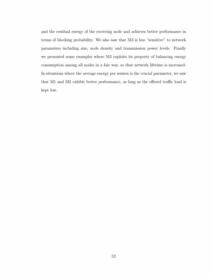
and the residual energy of the receiving node and achieves better performance in
terms of blocking probability. We also saw that M3 is less “sensitive” to network
parameters including size, node density and transmission power levels. Finally
we presented some examples where M3 exploits its property of balancing energy
consumption among all nodes in a fair way, so that network lifetime is increased.
In situations where the average energy per session is the crucial parameter, we saw
that M1 and M2 exhibit better performance, as long as the offered traffic load is
kept low.
52

Chapter 3
Energy-Efficient Routing of Connection-Oriented
Traffic, Part II: Limited Bandwidth Resources
3.1 Introduction
In the first part of our study on energy-efficient routing (chapter 2) we assumed
infinite bandwidth resources so that any node could access the wireless channel on
demand, without any need for contention and without causing any interference to
other neighboring nodes. A call request would be admitted to the system provided
a path existed with at least one transceiver available at every node. In a realistic
wireless system however, spectrum is scarce and links are bandwidth constrained
making the problem of efficient and interference-free sharing of common bandwidth
resources very crucial for the overall network performance. Depending on the
base technology used to isolate traffic from different stations, bandwidth resources
may be modeled by either transmission time-slots or frequency channels or CDMA
orthogonal codes. In this chapter, our focus is on the development of algorithms for
routing connection-oriented traffic under energy and bandwidth limitations. Every
node is assumed to have a sufficiently large number of transceivers so that calls are
53

never blocked due to unavailability of a transmitter or a receiver. We propose a
reservation-based scheme that supports end-to-end sessions based on the efficient
sharing of a set of distinct frequency channels and we investigate techniques of
jointly addressing the problem of power-sensitive route discovery and conflict-free
allocation of frequency channels to transmitting nodes.
Recall that wireless ad-hoc networks differ from other types of wireless archi-
tectures (e.g. cellular systems, wireless LANs, etc.) in that communication is not
always possible via a direct-hop link from the origin to the destination; in fact it
is very common to route traffic over multi-hop paths. A transmission by a node
gets received by all its one-hop neighbors causing interference to non-intended re-
cipients. By contrast, in wire-line networks where a link connecting two nodes is
exclusively used by these nodes without interfering with neighboring transmissions.
Hence, a channel access mechanism is required for the interference-free schedul-
ing of transmissions. However, the lack of complete connectivity among all nodes
allows more than one nodes to simultaneously use the channel without causing
conflicts, provided they are spatially separated. Notice though, that the number
of simultaneous transmissions that can take place interference-free is not known a
priori and can only be determined by complete knowledge of the set of network pa-
rameters consisting of the topology map, transmission power, number of available
frequency channels, transceivers per node and other information.
A fundamental design choice on the multiple access scheme to be used depends
on the type of workload that is carried by the network. Multiple access techniques
that have been extensively used in packet-based networks are generally classified
into two broad categories: random access schemes and reservation-based mecha-
nisms. Random access schemes (e.g. Aloha, CSMA, etc.) are more appropriate
54

for single hop access and are typically based on a simple or modified “free-for-
all” approach, in which nodes send packets either immediately or after sensing
the carrier and utilize sophisticated algorithms for retransmitting collided packets.
On the other extreme, reservation-based schemes (TDMA, FDMA, CDMA, etc.)
utilize a perfectly scheduled approach (it could be static or dynamic) in which
according to some rules nodes may transmit or receive at specific intervals and on
reserved frequencies. Random access schemes are more appropriate for networks
carrying datagram traffic (in which for example it is more efficient to negotiate link
access on a packet by packet basis). By contrast, in systems carrying connection-
oriented traffic stations generate steady streams of information and it is preferable
to allocate part of the link to the source for its exclusive use, thus avoiding the
additional overhead of negotiating link access for every packet in the stream. At
the same time, and in order to support connection-oriented traffic, nodes must be
capable of receiving and transmitting simultaneously, necessitating therefore the
use of sufficiently separated frequency channels.
Although the use of a frequency division multiple access scheme (FDMA) in-
troduces the difficult problem of assigning non-interfering frequencies to trans-
mitting nodes, it is the most appropriate for our problem. We could possibly
eliminate this difficulty by considering a system based on code division multi-
ple access (CDMA), in which quasi-orthogonal codes would be used. However,
in direct-sequence CDMA systems nodes are not allowed to handle simultaneous
transmission and reception in the same frequency band. It would also be of inter-
est to study systems that use time-division multiple access (TDMA), rather than
multiple transceivers, to support multiple sessions simultaneously. In fact such
systems have been studied [13, 14] in the context of scheduling problems and for
55
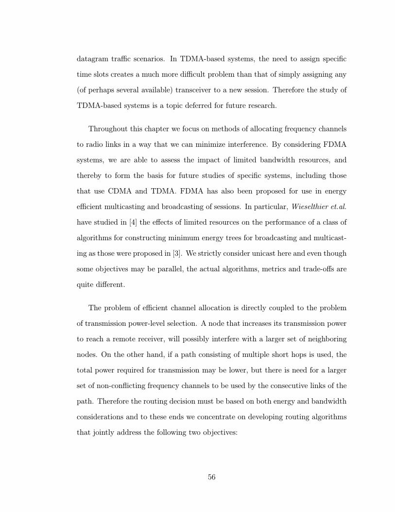
datagram traffic scenarios. In TDMA-based systems, the need to assign specific
time slots creates a much more difficult problem than that of simply assigning any
(of perhaps several available) transceiver to a new session. Therefore the study of
TDMA-based systems is a topic deferred for future research.
Throughout this chapter we focus on methods of allocating frequency channels
to radio links in a way that we can minimize interference. By considering FDMA
systems, we are able to assess the impact of limited bandwidth resources, and
thereby to form the basis for future studies of specific systems, including those
that use CDMA and TDMA. FDMA has also been proposed for use in energy
efficient multicasting and broadcasting of sessions. In particular, Wieselthier et.al.
have studied in [4] the effects of limited resources on the performance of a class of
algorithms for constructing minimum energy trees for broadcasting and multicast-
ing as those were proposed in [3]. We strictly consider unicast here and even though
some objectives may be parallel, the actual algorithms, metrics and trade-offs are
quite different.
The problem of efficient channel allocation is directly coupled to the problem
of transmission power-level selection. A node that increases its transmission power
to reach a remote receiver, will possibly interfere with a larger set of neighboring
nodes. On the other hand, if a path consisting of multiple short hops is used, the
total power required for transmission may be lower, but there is need for a larger
set of non-conflicting frequency channels to be used by the consecutive links of the
path. Therefore the routing decision must be based on both energy and bandwidth
considerations and to these ends we concentrate on developing routing algorithms
that jointly address the following two objectives:
56
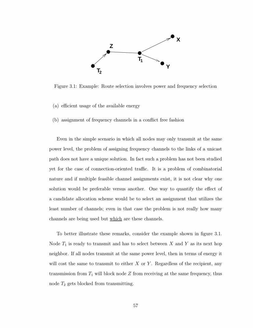
��������
���
���
����
����
��������
��������������������
��������������������
��������������
T
X
Y
Z
T
1
2
Figure 3.1: Example: Route selection involves power and frequency selection
(a) efficient usage of the available energy
(b) assignment of frequency channels in a conflict free fashion
Even in the simple scenario in which all nodes may only transmit at the same
power level, the problem of assigning frequency channels to the links of a unicast
path does not have a unique solution. In fact such a problem has not been studied
yet for the case of connection-oriented traffic. It is a problem of combinatorial
nature and if multiple feasible channel assignments exist, it is not clear why one
solution would be preferable versus another. One way to quantify the effect of
a candidate allocation scheme would be to select an assignment that utilizes the
least number of channels; even in that case the problem is not really how many
channels are being used but which are these channels.
To better illustrate these remarks, consider the example shown in figure 3.1.
Node T1 is ready to transmit and has to select between X and Y as its next hop
neighbor. If all nodes transmit at the same power level, then in terms of energy it
will cost the same to transmit to either X or Y . Regardless of the recipient, any
transmission from T1 will block node Z from receiving at the same frequency, thus
node T2 gets blocked from transmitting.
57
If we allow the transmitting node to adjust its power depending on the intended
receiver, we can associate each candidate link with a cost metric that captures both
the energy and the interference cost. Consider again the example of figure 3.1 but
now with the possibility to transmit at multiple power levels depending on the
distance from the intended recipient. Denote by d(A,B) the distance between
any two nodes A and B. If d(T1, Y ) < d(T1, X) the transmission power is lower
if Y is selected as the receiver. Additionally, if d(T1, Y ) < d(T1, Z) < d(T1, X)
a transmission from T1 to Y does not prohibit T2 from transmitting at the same
frequency, whereas this is not the case if T1 transmits to X. Clearly, such situations
occur frequently in the context of wireless ad-hoc topologies and our objective is
to define a method for modeling interference which also takes into account the
transmission power level.
The remaining of the chapter is organized as follows. In the next section we
extend our wireless network model of chapter 2 to address interference effects. We
define a set of rules regarding conflict avoidance situations and in the sequel we
discuss the difficulties encountered in developing an optimized solution and we
provide an overview of our approach. We continue with a detailed description of
our proposed algorithms and study their properties and implementation require-
ments. In the final section we present a detailed performance analysis, based on
our simulation model and wrap up the chapter with a summary of conclusions.
3.2 Interference model
The network topology is modeled by a directed graph G = (V,E) where the ele-
ments of V represent the network nodes and each directed edge (i, j) ∈ E denotes
58
a radio communication link between the communication nodes i and j. Similarly
to our model defined in chapter 2 we denote by R(x) all one hop neighbors of node
x, ie all nodes that are located within the transmission range of x defined as a
circle centered in x with radius equal to dmax.
A total of m frequency channels are available for use, denoted by f1, f2, · · · , fm.
Each node i maintains a set of channel status vectors, one for each node j ∈ R(i).
These vectors consist of 0’s and 1’s that indicate whether a channel is free or
blocked respectively. Therefore the channel-status vector of node i for transmission
to node j will be given by:
f (i,j) = [f (i,j)(1), · · · , f (i,j)(m)] (3.1)
where for all k we define:
f (i,j)(k) =
1 if kth channel is available
0 otherwise(3.2)
In order to admit a new session request, a path p must exist from the source
to the destination, such that all nodes i ∈ p have at least one frequency channel
available for transmission; moreover a conflict free channel allocation must exist
that satisfies the following requirements:
– A node cannot transmit and receive in the same frequency
– A node cannot simultaneously receive more than one signals in the same
frequency
– A node cannot transmit simultaneously to more than one neighboring nodes
(we strictly consider unicast here; in a broadcast scenario this would an
acceptable and in fact encouraged situation).
59
As a result of these conditions, a transmission over any link may prevent a subset
of neighboring nodes from transmitting at the same frequency and at a certain
power level. In order to determine conflict-free channel assignments, nodes must
be aware of the frequencies they are allowed to use (along with the allowable power
levels). We define a simplified interference model in which a receiver is assumed
to ignore interference from simultaneous neighboring transmissions if the distance
from the location of the interfering source exceeds dmax. In particular, we make
a binary decision of whether we can allow or not a transmission, without detailed
calculation of SIR at every node, since such a task would increase the complexity
of an already difficult problem. Nonetheless, in principle, a more accurate model
for interference can be incorporated in our model.
Under these considerations, a transmission over link (A,B) using frequency fk
results in the blocking of the following neighboring links:
– Primary conflicts:
P1: Any link (v, A), v ∈ R(A), because A cannot receive and transmit at
the same frequency.
P2: Any link (A, v), v ∈ R(A), because A cannot transmit to more than
one nodes simultaneously.
P3: Any link (v, B), v ∈ R(B), because B cannot receive from more than
one nodes simultaneously.
P4: Any link (B, v), v ∈ R(B), because B cannot transmit and receive at
the same frequency.
– Secondary conflicts:
60
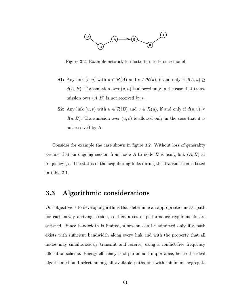
A B
C
D L
K
Figure 3.2: Example network to illustrate interference model
S1: Any link (v, u) with u ∈ R(A) and v ∈ R(u), if and only if d(A, u) ≥
d(A,B). Transmission over (v, u) is allowed only in the case that trans-
mission over (A,B) is not received by u.
S2: Any link (u, v) with u ∈ R(B) and v ∈ R(u), if and only if d(u, v) ≥
d(u,B). Transmission over (u, v) is allowed only in the case that it is
not received by B.
Consider for example the case shown in figure 3.2. Without loss of generality
assume that an ongoing session from node A to node B is using link (A,B) at
frequency fk. The status of the neighboring links during this transmission is listed
in table 3.1.
3.3 Algorithmic considerations
Our objective is to develop algorithms that determine an appropriate unicast path
for each newly arriving session, so that a set of performance requirements are
satisfied. Since bandwidth is limited, a session can be admitted only if a path
exists with sufficient bandwidth along every link and with the property that all
nodes may simultaneously transmit and receive, using a conflict-free frequency
allocation scheme. Energy-efficiency is of paramount importance, hence the ideal
algorithm should select among all available paths one with minimum aggregate
61
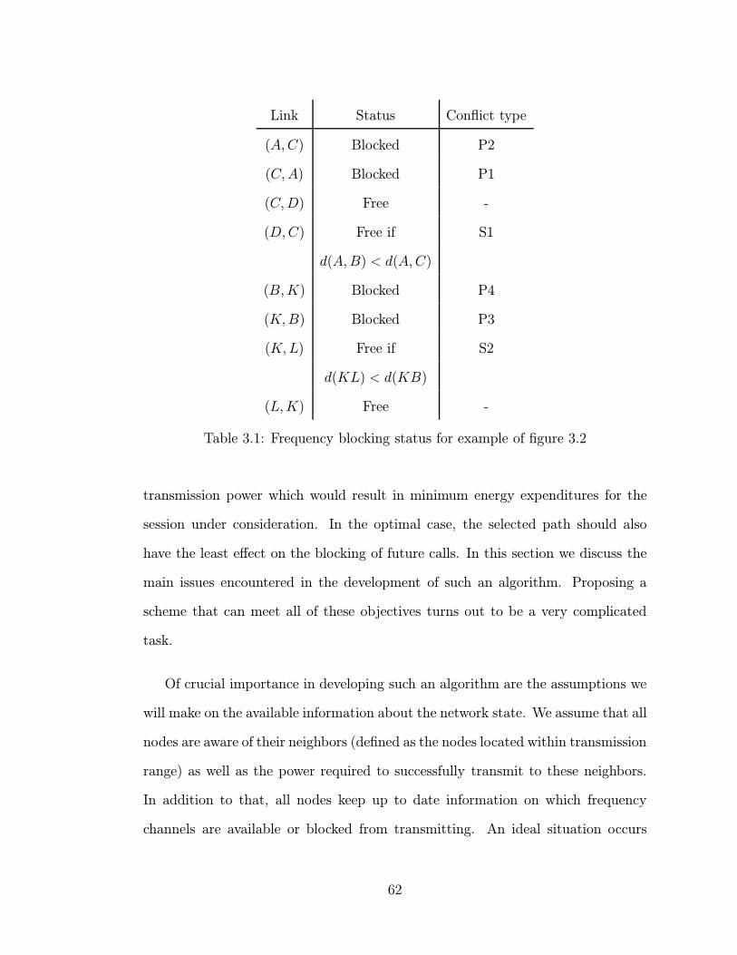
Link Status Conflict type
(A,C) Blocked P2
(C,A) Blocked P1
(C,D) Free -
(D,C) Free if S1
d(A,B) < d(A,C)
(B,K) Blocked P4
(K,B) Blocked P3
(K,L) Free if S2
d(KL) < d(KB)
(L,K) Free -
Table 3.1: Frequency blocking status for example of figure 3.2
transmission power which would result in minimum energy expenditures for the
session under consideration. In the optimal case, the selected path should also
have the least effect on the blocking of future calls. In this section we discuss the
main issues encountered in the development of such an algorithm. Proposing a
scheme that can meet all of these objectives turns out to be a very complicated
task.
Of crucial importance in developing such an algorithm are the assumptions we
will make on the available information about the network state. We assume that all
nodes are aware of their neighbors (defined as the nodes located within transmission
range) as well as the power required to successfully transmit to these neighbors.
In addition to that, all nodes keep up to date information on which frequency
channels are available or blocked from transmitting. An ideal situation occurs
62
when “complete” information on the network state is available. Such information
includes the full connectivity map with detailed transmission power levels and the
frequency channels being used or blocked by every node. At the establishment
or termination of a call this information must be updated and be made available
either to all nodes or to some central coordinator. Even if we neglect the cost of
obtaining and maintaining complete information, the best possible solution would
involve the use of a greedy algorithm that would maximize an expected reward
function on a per call basis. In that case for example, the reward can be defined
either as the total transmission power required, or as a linear combination of total
power and number of blocked resources. Such a method requires the exhaustive
search of a large state space which grows exponentially with the network size and
therefore it is impractical except for trivially small networks.
Since it is extremely costly (in terms of overhead and time complexity) to main-
tain complete state information, an alternative approach would look for suboptimal
solutions that rely on local information in order to determine the routes to be used.
Local information can be acquired through the periodic exchange of control packets
between neighboring nodes. Similarly to the mechanisms developed for the case of
unlimited frequency channels (chapter 2), we examine heuristic algorithms that do
not require a complete information map and restrict the search to a significantly
smaller space. In particular, we can define link metrics that capture local param-
eters and use the Bellman-Ford algorithm to determine the minimum cost path.
Nevertheless, there is no direct way of predicting what blocking impact a specific
frequency channel might have on future calls. In fact the set of neighboring nodes
that get blocked is the same regardless of the choice of transmission frequency. In
the case of plentiful bandwidth resources, the existence of one transceiver along
63

����
������
������
���
���
��������
������
������
��������
���
���
��������
SD
f f f1 1 1
SD
f f f1 2 3
Figure 3.3: Two instances of the same path showing the available frequencies
every node in the path was sufficient to guarantee the availability of the path. By
incorporating such information into the link metrics (link cost was set to infinite
if one of the two edge nodes of the links had no transceivers available), the algo-
rithm would always determine a feasible path. Apparently, any finite cost path
was a candidate path for admitting the new session. If we were to follow a similar
approach for the case of limited frequency bands, there would be no guarantee
that a finite cost path would also be appropriate for establishing the session. The
existence of at least one available frequency channel in each link of a path does not
guarantee call admission; instead an interference-free allocation of channels must
be determined. Such an allocation is not directly related to the number of channels
available for each node but rather to which are these channels. We illustrate our
point through a simple example shown in figure 3.3, where two instances of the
same path are depicted as well as the available channels of each link. We define our
link metric to be equal to the inverse of the number of available channels so that
we favor links with multiple free bands. Both cases result in the same path cost;
however, only for the path on the left can we have interference-free transmission.
Another limitation is that the nodes of a path cannot select which frequency
to use (among the set of available channels) independently. For every channel
assignment made over one link, neighboring nodes that experience interference
must update their blocked-frequency table before they make their assignment.
64
Therefore a channel allocation algorithm must generate the frequency assignments
on a hop-by-hop basis.
Based on the above discussion and remarks our approach continues as follows.
We first present a class of heuristic algorithms that are easier to implement but
their performance has to be evaluated. We then discuss complexity issues of ex-
haustive search methods and propose two schemes that can be used as a common
comparison basis in relatively small network examples. A detailed performance
evaluation section follows in which the algorithms are compared and their most
significant features are discussed.
3.4 Heuristic algorithms
The heuristics we have proposed evolve in the following two stages:
– a minimum cost path (as measured by energy and blocked resources) is first
determined (referred to as the candidate path)
– if an interference-free channel assignment can be determined along that path,
the call request is admitted to the system.
3.4.1 Link metrics for determining minimum cost path
In this section, we propose the minimum power metric (MPM) and the power and
interference based metric (PIM) for determining the cost of the links.
(a) Minimum power metric (MPM)
MPM accounts for energy requirements only and is a direct measure of the
power needed to transmit over the specific link, provided that at least one frequency
65
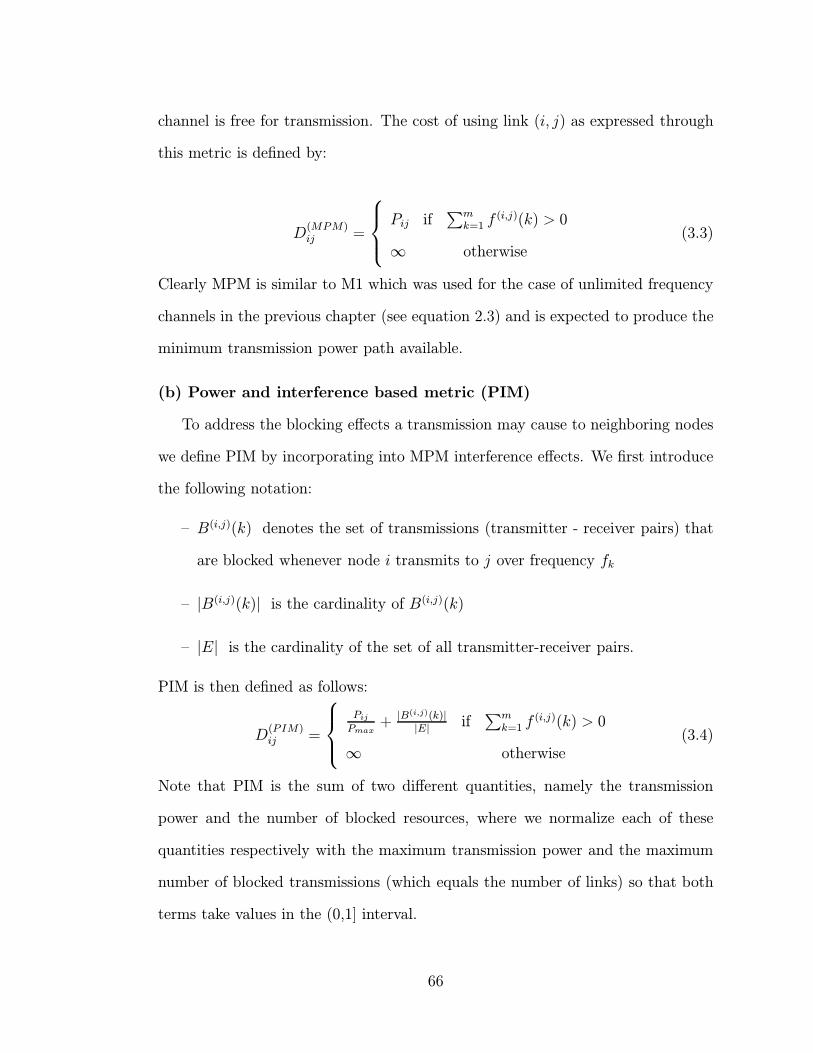
channel is free for transmission. The cost of using link (i, j) as expressed through
this metric is defined by:
D(MPM)ij =
Pij if∑m
k=1 f(i,j)(k) > 0
∞ otherwise(3.3)
Clearly MPM is similar to M1 which was used for the case of unlimited frequency
channels in the previous chapter (see equation 2.3) and is expected to produce the
minimum transmission power path available.
(b) Power and interference based metric (PIM)
To address the blocking effects a transmission may cause to neighboring nodes
we define PIM by incorporating into MPM interference effects. We first introduce
the following notation:
– B(i,j)(k) denotes the set of transmissions (transmitter - receiver pairs) that
are blocked whenever node i transmits to j over frequency fk
– |B(i,j)(k)| is the cardinality of B(i,j)(k)
– |E| is the cardinality of the set of all transmitter-receiver pairs.
PIM is then defined as follows:
D(PIM)ij =
PijPmax
+ |B(i,j)(k)||E| if
∑mk=1 f
(i,j)(k) > 0
∞ otherwise(3.4)
Note that PIM is the sum of two different quantities, namely the transmission
power and the number of blocked resources, where we normalize each of these
quantities respectively with the maximum transmission power and the maximum
number of blocked transmissions (which equals the number of links) so that both
terms take values in the (0,1] interval.
66

3.4.2 Frequency allocation algorithms
Once a candidate minimum cost path has been identified, an interference-free chan-
nel allocation must be determined for those nodes that will be transmitting. In
this section we discuss the details of two frequency allocation mechanisms:
– a heuristic that allocates channels to the links of the candidate path starting
from the origin and proceeding link-by-link towards the destination. We will
refer to it as the link-by-link greedy (LLG) frequency allocation algorithm
– a second heuristic that assumes complete knowledge of the candidate path
and allocates channels to its links starting with the most congested. We
will refer to it as the most congested link first (MCLF) frequency allocation
algorithm.
(a) Link-by-link greedy frequency allocation (LLG)
The motivation for the link-by-link greedy allocation scheme comes from the
use of similar greedy channel allocation schemes in linear cellular networks. Chan-
nel allocation is performed along the candidate path in a hop-by-hop manner,
starting from the origin node and moving towards the destination, selecting an
available channel for each link (and updating blocked frequencies after each allo-
cation). Since the candidate path is a finite cost path, all its nodes have initially
at least one frequency channel available for use. However, as the step by step
reservation proceeds, a node may run out of frequencies due to blocking by neigh-
boring transmissions and if a link is not allocated a frequency successfully the call
is blocked.
We first illustrate how this scheme operates by providing a simple example.
Consider an isolated path from the source node S to the destination D as shown
67
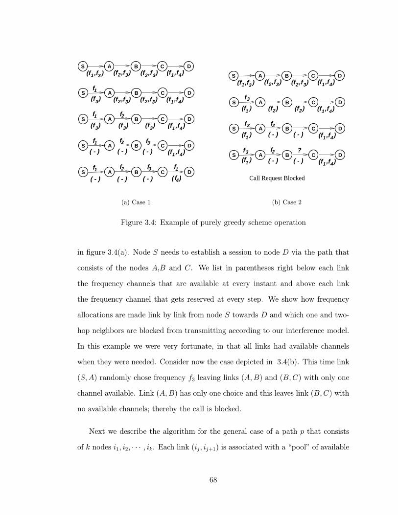
A B C DS
A B C DS
A B C DS
1f
1f
1f 1f
1f
f2
f2
f2
f3
f3
(f ,f )2 3
(f ,f )2 3 (f ,f )2 3
A B C DS
(f ,f )1 4
(f ,f )1 4(f )3
(f )3 (f )3 (f )3
(f ,f )1 4
(f ,f )1 4
f4( )A B C DS
(f ,f )(f ,f )1 3 2 3
( - ) ( - ) ( - )
( - )( - )( - )
(a) Case 1
A B C DS
A B C DS
f2
f2
(f ,f )2 3 (f ,f )1 4
(f ,f )1 4
(f ,f )1 4
(f ,f )1 4
A B C DS
A B C DS
2(f ) 2(f )
3f
3f
(f )1
(f )1
3f(f )1
(f ,f )(f ,f )1 3 2 3
( - ) ( - )
( - )( - )
?
Call Request Blocked
(b) Case 2
Figure 3.4: Example of purely greedy scheme operation
in figure 3.4(a). Node S needs to establish a session to node D via the path that
consists of the nodes A,B and C. We list in parentheses right below each link
the frequency channels that are available at every instant and above each link
the frequency channel that gets reserved at every step. We show how frequency
allocations are made link by link from node S towards D and which one and two-
hop neighbors are blocked from transmitting according to our interference model.
In this example we were very fortunate, in that all links had available channels
when they were needed. Consider now the case depicted in 3.4(b). This time link
(S,A) randomly chose frequency f3 leaving links (A,B) and (B,C) with only one
channel available. Link (A,B) has only one choice and this leaves link (B,C) with
no available channels; thereby the call is blocked.
Next we describe the algorithm for the general case of a path p that consists
of k nodes i1, i2, · · · , ik. Each link (ij , ij+1) is associated with a “pool” of available
68
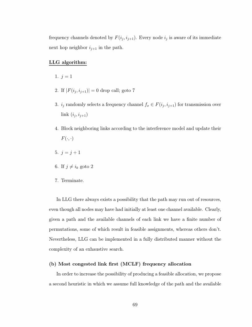
frequency channels denoted by F (ij, ij+1). Every node ij is aware of its immediate
next hop neighbor ij+1 in the path.
LLG algorithm:
1. j = 1
2. If |F (ij, ij+1)| = 0 drop call; goto 7
3. ij randomly selects a frequency channel fx ∈ F (ij, ij+1) for transmission over
link (ij , ij+1)
4. Block neighboring links according to the interference model and update their
F (·, ·)
5. j = j + 1
6. If j 6= ik goto 2
7. Terminate.
In LLG there always exists a possibility that the path may run out of resources,
even though all nodes may have had initially at least one channel available. Clearly,
given a path and the available channels of each link we have a finite number of
permutations, some of which result in feasible assignments, whereas others don’t.
Nevertheless, LLG can be implemented in a fully distributed manner without the
complexity of an exhaustive search.
(b) Most congested link first (MCLF) frequency allocation
In order to increase the possibility of producing a feasible allocation, we propose
a second heuristic in which we assume full knowledge of the path and the available
69
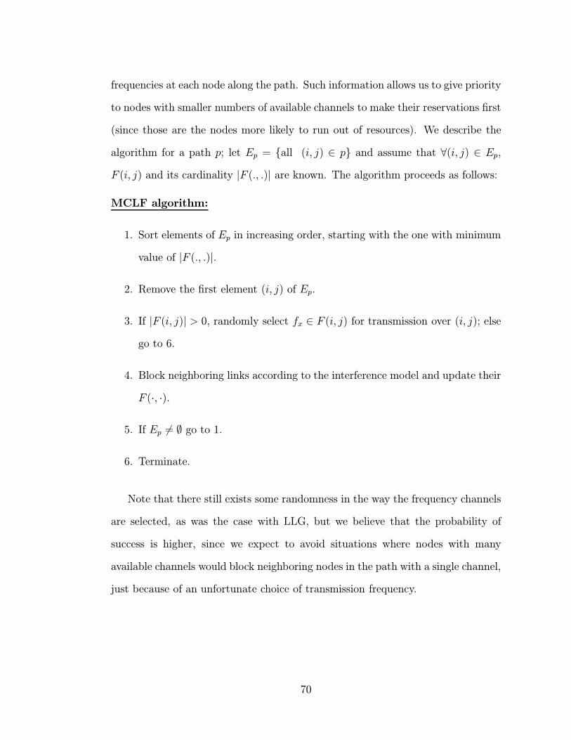
frequencies at each node along the path. Such information allows us to give priority
to nodes with smaller numbers of available channels to make their reservations first
(since those are the nodes more likely to run out of resources). We describe the
algorithm for a path p; let Ep = {all (i, j) ∈ p} and assume that ∀(i, j) ∈ Ep,
F (i, j) and its cardinality |F (., .)| are known. The algorithm proceeds as follows:
MCLF algorithm:
1. Sort elements of Ep in increasing order, starting with the one with minimum
value of |F (., .)|.
2. Remove the first element (i, j) of Ep.
3. If |F (i, j)| > 0, randomly select fx ∈ F (i, j) for transmission over (i, j); else
go to 6.
4. Block neighboring links according to the interference model and update their
F (·, ·).
5. If Ep 6= ∅ go to 1.
6. Terminate.
Note that there still exists some randomness in the way the frequency channels
are selected, as was the case with LLG, but we believe that the probability of
success is higher, since we expect to avoid situations where nodes with many
available channels would block neighboring nodes in the path with a single channel,
just because of an unfortunate choice of transmission frequency.
70
3.5 Exhaustive search mechanisms
As was discussed in section 3.3, if complete network state information is considered
an exhaustive search among all possible allocations can determine the path and as-
signment that maximizes a per-call reward function. A path from the source to the
destination node is characterized as available if an interference-free frequency chan-
nel assignment exists. If the reward function is defined as the total transmission
power for using the path, our mechanism should search among all available paths
and return the minimum power path. Alternatively, we could consider a reward
function as a combination of power and amount of blocked resources. In any case,
such a technique is still greedy in that it optimizes the reward produced by a given
call, based on the current network state. We describe next an implementation of
an exhaustive search, referred to as ExSrch, that determines the available path
with the maximum reward. We also consider a scheme that restricts the search to
the candidate path. Note that both schemes are useful for performance evaluation
purposes but their huge complexity prohibits their implementation in an actual
system.
3.5.1 Complete exhaustive search implementation (ExS-
rch)
1. A call arrives at node i ∈ V destined for node j ∈ V
2. Given the network state consider the subgraph G′ = (V,E′) where E′ ⊂ E
such that: E′ = {(i, j) ∈ E|∑m
k=1 f(i,j)(k) > 0} .
3. Find all available paths ∈ G′ from i to j (with their corresponding frequency
allocations).
71
4. If no path can be found drop the call and go to 7; otherwise assign the call
to the path that maximizes the reward.
5. According to the interference model block the nodes that should not transmit
at the same frequency.
6. Update network state.
7. Terminate.
The main advantage of the exhaustive search is that it always determines the
minimum cost path among all available paths at the time the new session arrives to
the system. However, performing an exhaustive search over a random (and possibly
varying) network topology is an extremely complex task. It is rather impractical
to think of it as a possible solution to our problem and will only be used as a basis
for comparison. Even in that case it can only be applied to simple examples with
few nodes, therefore it can not lead to significant conclusions. However, in order
to illustrate how complex it may be to get to the optimal solution consider the
following example:
Example:
Consider the topologies shown in figure 3.5. If these nodes are deployed in a
100 × 100 square grid and the transmission range is set to dmax = 35 units (fig-
ure 3.5.a), the total number of paths between all possible source-destination pairs
is 642. Assume that a new call arrives at node 4 destined for node 6. There exist
9 possible paths connecting node 4 to node 6. Of these paths, 2 consist of 3 links,
4 of 4 links and 3 of 5 links. If the number of frequency channels in the network
were 5, we could have a total number of 35× 2 + 45× 4 + 55× 3 = 13957 frequency
72

0
1
2
3
4
5
6
7
8
9
(a) dmax = 35
0
1
2
3
4
5
6
7
8
9
(b) dmax = 40
Figure 3.5: Network topologies of example 1
allocations along these paths. Due to interference constraints, some of these allo-
cations are not permissible and of course a lot of them might not be feasible due
to blocked frequencies or other on going transmissions, but we still have to search
and evaluate a large number of possibilities. If the network connectivity is denser,
the search space increases rapidly. For example the maximum transmission power
is augmented to make the transmission range equal to dmax = 40 (figure 3.5.b),
the total number of paths for all origin-destination pairs in the network becomes
6090. For the same source and destination (4,6) we now have 93 paths and nearly
one million combinations.
3.5.2 Exhaustive search of minimum-cost path (ESMP)
Exhaustive search can also be limited in the minimum cost path in order to reduce
the size of the solution space. We propose the Exhaustive Search of Minimum-cost
Path (ESMP) scheme, which searches among all possible channel allocations of the
73
candidate path and selects an interference-free assignment to carry the session.
Oftentimes there may exist multiple such allocations and ESMP will select the
first one to be discovered, for no allocation is classified as better or worse than
any other. Since the whole state space is searched, if no allocation can be found
there doesn’t exist one along the specific path, given the current network state;
hence the session is not admitted to the system. In a sense, ESMP operates as
an admission control algorithm which admits a new session only if it can route it
along the minimum cost path. Moreover, since ESMP only examines the minimum
cost path, it can form an important comparison metric for the evaluation of LLG
and MCLF.
Compared to ExSrch, ESMP is less complex, even though it still has to perform
a search among all possible frequency permutations. Given the number of nodes N
in the network and the number of frequency channels m, the worst case scenario
would occur for a path of maximum length (N − 1 links) if the search had to
examine all possible allocations, ie a total of (N−1)m possibilities. ESMP remains
an impractical method for large topologies especially since the search space grows
exponentially with the network size. Thereby, our comparison between ExSrch,
ESMP, LLG and MCLF is limited to small-sized topologies.
3.6 Performance analysis
For the purposes of performance evaluation of the algorithms presented in this
chapter, we have extended the simulation model developed for the algorithms in
chapter 2 (described in appendix A) to support the case of limited frequency chan-
nels as well. We have incorporated the interference model and have implemented
74
all the algorithms presented in this current chapter.
The assumptions that were made in chapter 2 regarding the traffic models, the
node topologies (randomly generated networks) and the performance measures
continue to hold. The enhanced model differs from before in that there is no limit
in the number of transceivers per node and as a consequence a call may be blocked
only due to unavailability of frequency channels.
3.6.1 Comparison of frequency allocation heuristics versus
exhaustive search mechanisms
We have evaluated the performance of the heuristics for frequency channel alloca-
tion and compared the results against those provided by an exhaustive search. Due
to the enormous amount of computation that is required for the case of exhaustive
search, we have limited our comparison to two sample topologies of 10 nodes. In
each example we consider use of the MPM metric for link cost assignment and
evaluate the heuristics for the cases of mf = 3 and mf = 6 frequency channels.
Example 1
In this example we consider the topology examined in section 3.5.1, shown
in figure 3.5, which consists of 10 nodes. We evaluate two different instances of
the same network that correspond to maximum transmission range of dmax = 35
(fig. 3.5(a)) and dmax = 40 (fig. 3.5(b)) units respectively. Performance results for
this example are summarized in Tables 3.2 (blocking probability) and 3.3 (energy
per session).
We do observe that in most of the situations the exhaustive search (ExSrch)
provides better performance in terms of blocking probability, which would be ex-
75

mf = 3 mf = 6
λ dmax = 35 dmax = 40 dmax = 35 dmax = 40 Algorithm
0.193 0.129 0.006 0.005 ExSrch
0.1 0.220 0.190 0.013 0.009 ESMP
0.224 0.187 0.013 0.010 MCLF
0.226 0.197 0.015 0.013 LLG
0.442 0.373 0.110 0.075 ExSrch
0.3 0.442 0.399 0.122 0.093 ESMP
0.446 0.409 0.129 0.101 MCLF
0.457 0.413 0.134 0.104 LLG
0.556 0.506 0.258 0.202 ExSrch
0.5 0.555 0.519 0.250 0.208 ESMP
0.559 0.521 0.253 0.218 MCLF
0.565 0.528 0.262 0.209 LLG
0.634 0.593 0.357 0.297 ExSrch
0.7 0.627 0.594 0.359 0.304 ESMP
0.626 0.589 0.362 0.297 MCLF
0.629 0.595 0.368 0.325 LLG
Table 3.2: Blocking probabilities for topology of Example 1
76

mf = 3 mf = 6
λ dmax = 35 dmax = 40 dmax = 35 dmax = 40 Algorithm
1.409 1.472 1.416 1.393 ExSrch
0.1 1.329 1,326 1.406 1,387 ESMP
1.336 1.306 1.389 1.376 MCLF
1.315 1.309 1.403 1.382 LLG
1.364 1.489 1.430 1.454 ExSrch
0.3 1.252 1.287 1.379 1.371 ESMP
1.276 1.278 1.396 1.374 MCLF
1.236 1.237 1.346 1.380 LLG
1.290 1.454 1.466 1.596 ExSrch
0.5 1.194 1.274 1.361 1.391 ESMP
1.170 1.252 1.352 1.401 MCLF
1.177 1.235 1.324 1.370 LLG
1.232 1.457 1.426 1.393 ExSrch
0.7 1.148 1.250 1.355 1.396 ESMP
1.143 1.236 1.344 1.381 MCLF
1.108 1.189 1.342 1.377 LLG
Table 3.3: Energy per session for topology of Example 1
77
pected since for every incoming request this method explores all routing possibili-
ties and blocks the call only if no path and frequency allocation exists. Of course
this comes at the cost of higher Es since the call admission is now restricted to the
minimum cost path.
It is remarkable to point out that in some isolated situations we have observed
that either the ESMP scheme or one of the heuristics (LLG or MCLF) resulted
in better performance than the ExSrch. For example, in the case of dmax = 35,
λ = 0.5 and m = 6, ESMP and MCLF provided lower blocking than ExSrch. Simi-
larly, for dmax = 35, λ = 0.7 and m = 3, ExSrch had the worst performance among
all methods. Even though such a behavior was not expected, it is a consequence
of the fact that the ExSrch does not guarantee a global optimum since it works on
a per call basis. In fact, a global optimum would be obtainable only if complete
knowledge of the traffic pattern was available prior to the beginning of the simula-
tion. Of course, for a certain call and given the current network state, no heuristic
can provide a better solution than the ExSrch. Sometimes however, there may ex-
ist more than one valid frequency assignments along the minimum cost path; every
valid assignment though, has the same effect on blocking of neighboring nodes (ie
the number of blocked transmissions does not depend on the selected channel but
it depends only on the power level and the receiving node) but may have different
effect on future calls, depending on the future traffic characteristics. Hence, it is
possible that by accepting a call via the exhaustive search (a call that would have
been otherwise blocked via one of the heuristics) future calls may be adversely
affected (ie in a way worse than that of the heuristic). Of course, all the heuristics
work on a per call basis, so on the average scale such situations are not very likely
to happen and as our results indicate they do happen only in few cases, which is
78

consistent with the above explanation.
Although our performance results have indicated so far that in terms of blocking
probability ExSrch has on an average scale the best performance, it is interesting
to analyze how well or how bad the heuristics perform compared to it. Note that
on an average scale ESMP performs better than the two heuristics, with MCLF
coming next and LLG exhibiting the highest values of Pb. The results of table 3.2
indicate that when the transmission range increases, ESMP and the two heuristics
perform much worse than ExSrch. Such a behavior could be expected since even
a small increase in the transmission range results in a large number of new paths
and ExSrch is the only scheme that explores all possible paths between the origin
and the destination.
It is also of interest to observe the difference between the worst and best per-
forming algorithm for each set of arrival rates. For the case of m = 3, when the
traffic load is light there is significant difference in the values of Pb between ExSrch
and the rest, whereas for heavy traffic they are pretty close. On the other hand for
m = 6 the difference seems to be greater for heavy traffic, which is more intuitive
since it would be expected that the heuristics would perform less poorly when
traffic is light. An explanation that can be applicable for the case of m = 3 is that
because of the very small number of channels, it becomes less likely to determine
a feasible assignment along the minimum power path, since typically this would
rather be a multiple hop path; by contrast the ExSrch has the flexibility of using
higher power paths, even the highest available (which could be a long direct trans-
mission) as long as a channel assignment can be found. If we look at the values of
Es (table 3.3) our explanation is verified from the increased values of Es that the
ExSrch causes.
79
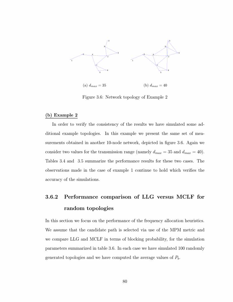
0
1
2
3
4
5
6
7
8
9
(a) dmax = 35
0
1
2
3
4
5
6
7
8
9
(b) dmax = 40
Figure 3.6: Network topology of Example 2
(b) Example 2
In order to verify the consistency of the results we have simulated some ad-
ditional example topologies. In this example we present the same set of mea-
surements obtained in another 10-node network, depicted in figure 3.6. Again we
consider two values for the transmission range (namely dmax = 35 and dmax = 40).
Tables 3.4 and 3.5 summarize the performance results for these two cases. The
observations made in the case of example 1 continue to hold which verifies the
accuracy of the simulations.
3.6.2 Performance comparison of LLG versus MCLF for
random topologies
In this section we focus on the performance of the frequency allocation heuristics.
We assume that the candidate path is selected via use of the MPM metric and
we compare LLG and MCLF in terms of blocking probability, for the simulation
parameters summarized in table 3.6. In each case we have simulated 100 randomly
generated topologies and we have computed the average values of Pb.
80
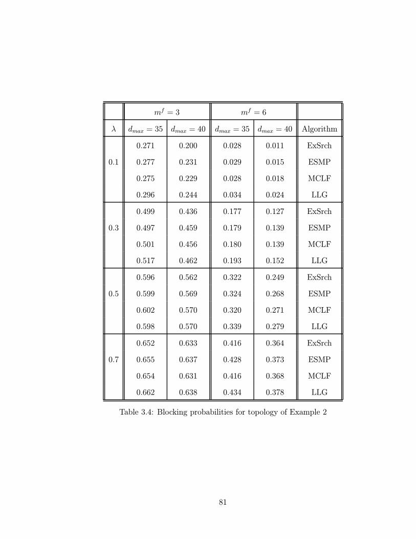
mf = 3 mf = 6
λ dmax = 35 dmax = 40 dmax = 35 dmax = 40 Algorithm
0.271 0.200 0.028 0.011 ExSrch
0.1 0.277 0.231 0.029 0.015 ESMP
0.275 0.229 0.028 0.018 MCLF
0.296 0.244 0.034 0.024 LLG
0.499 0.436 0.177 0.127 ExSrch
0.3 0.497 0.459 0.179 0.139 ESMP
0.501 0.456 0.180 0.139 MCLF
0.517 0.462 0.193 0.152 LLG
0.596 0.562 0.322 0.249 ExSrch
0.5 0.599 0.569 0.324 0.268 ESMP
0.602 0.570 0.320 0.271 MCLF
0.598 0.570 0.339 0.279 LLG
0.652 0.633 0.416 0.364 ExSrch
0.7 0.655 0.637 0.428 0.373 ESMP
0.654 0.631 0.416 0.368 MCLF
0.662 0.638 0.434 0.378 LLG
Table 3.4: Blocking probabilities for topology of Example 2
81
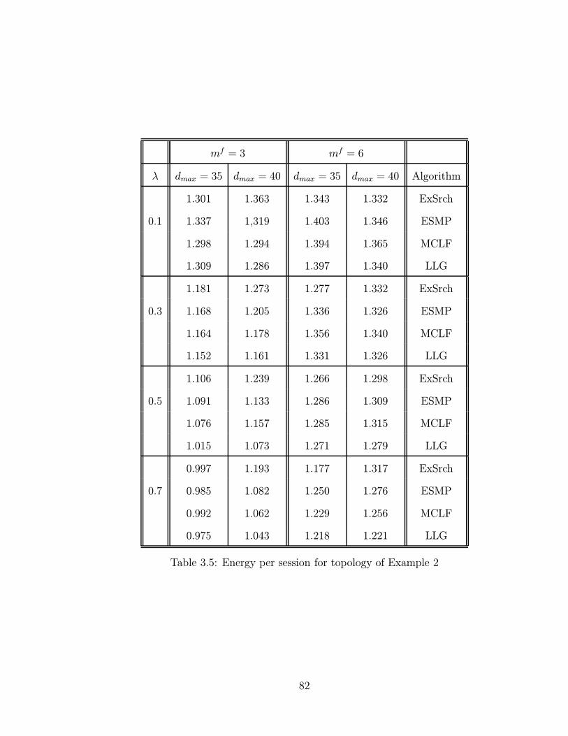
mf = 3 mf = 6
λ dmax = 35 dmax = 40 dmax = 35 dmax = 40 Algorithm
1.301 1.363 1.343 1.332 ExSrch
0.1 1.337 1,319 1.403 1.346 ESMP
1.298 1.294 1.394 1.365 MCLF
1.309 1.286 1.397 1.340 LLG
1.181 1.273 1.277 1.332 ExSrch
0.3 1.168 1.205 1.336 1.326 ESMP
1.164 1.178 1.356 1.340 MCLF
1.152 1.161 1.331 1.326 LLG
1.106 1.239 1.266 1.298 ExSrch
0.5 1.091 1.133 1.286 1.309 ESMP
1.076 1.157 1.285 1.315 MCLF
1.015 1.073 1.271 1.279 LLG
0.997 1.193 1.177 1.317 ExSrch
0.7 0.985 1.082 1.250 1.276 ESMP
0.992 1.062 1.229 1.256 MCLF
0.975 1.043 1.218 1.221 LLG
Table 3.5: Energy per session for topology of Example 2
82
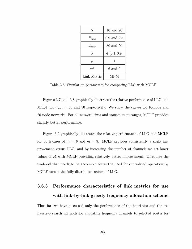
N 10 and 20
Pmax 0.9 and 2.5
dmax 30 and 50
λ ∈ [0.1, 0.9]
µ 1
mf 6 and 9
Link Metric MPM
Table 3.6: Simulation parameters for comparing LLG with MCLF
Figures 3.7 and 3.8 graphically illustrate the relative performance of LLG and
MCLF for dmax = 30 and 50 respectively. We show the curves for 10-node and
20-node networks. For all network sizes and transmission ranges, MCLF provides
slightly better performance.
Figure 3.9 graphically illustrates the relative performance of LLG and MCLF
for both cases of m = 6 and m = 9. MCLF provides consistently a slight im-
provement versus LLG, and by increasing the number of channels we get lower
values of Pb with MCLF providing relatively better improvement. Of course the
trade-off that needs to be accounted for is the need for centralized operation by
MCLF versus the fully distributed nature of LLG.
3.6.3 Performance characteristics of link metrics for use
with link-by-link greedy frequency allocation scheme
Thus far, we have discussed only the performance of the heuristics and the ex-
haustive search methods for allocating frequency channels to selected routes for
83

0.1 0.2 0.3 0.4 0.5 0.6 0.7 0.8 0.90
0.1
0.2
0.3
0.4
0.5
0.6
0.7
New Call Arrival Rate (Calls/node/time unit)
Blo
ckin
g P
roba
bilit
y (P
b)
Blocking Prob. vs Offered Load: dmax
=30, Pmax
=0.9, mf=6
LLG, N=10 MCLF, N=10LLG, N=20 MCLF, N=20
N=10
N=20
Figure 3.7: Comparison of LLG, MCLF through blocking probability, dmax = 30
0.1 0.2 0.3 0.4 0.5 0.6 0.7 0.8 0.90
0.1
0.2
0.3
0.4
0.5
0.6
0.7
New Call Arrival Rate (Calls/node/time unit)
Blo
ckin
g P
roba
bilit
y (P
b)
Blocking Prob. vs Offered Load: dmax
=50, Pmax
=2.5, mf=6
LLG, N=10 MCLF, N=10LLG, N=20 MCLF, N=20
N=10
N=20
Figure 3.8: Comparison of LLG, MCLF through blocking probability, dmax = 50
84
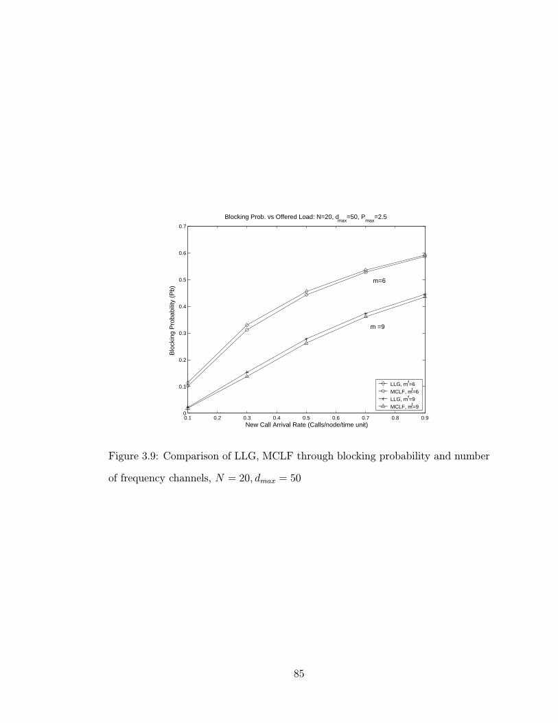
0.1 0.2 0.3 0.4 0.5 0.6 0.7 0.8 0.90
0.1
0.2
0.3
0.4
0.5
0.6
0.7
New Call Arrival Rate (Calls/node/time unit)
Blo
ckin
g P
roba
bilit
y (P
b)
Blocking Prob. vs Offered Load: N=20, dmax
=50, Pmax
=2.5
LLG, mf=6 MCLF, mf=6LLG, mf=9 MCLF, mf=9
m =9
m=6
Figure 3.9: Comparison of LLG, MCLF through blocking probability and number
of frequency channels, N = 20, dmax = 50
85
admitting new calls. In all the experiments we considered the link metric to be
given by MPM (equation 3.3). In this section we evaluate the relative perfor-
mance of MPM and PIM metrics for joint use with LLG as a channel allocation
algorithm. Figures 3.10 – 3.15 illustrate graphically the relative performance of
MPM and PIM. For each set of values of λ, dmax and N , we have run simulations
for 100 randomly generated topologies and we have computed the average values
of our performance measures, namely Pb, Es and Y . Table 3.7 summarizes the
simulation parameters for the results presented in this section.
N 10 and 20
Pmax 0.9 and 2.5
dmax 30 and 50
λ ∈ [0.1, 0.9]
µ 1
mf 6
Table 3.7: Simulation parameters for comparing MPM with PIM
From the graphs shown in figures 3.10 and 3.11 we observe that use of PIM
provides better performance in terms of blocking probability in all of the cases.
Note that when the network becomes denser (larger N), Pb increases. It is also
of interest to point out that PIM achieves better improvement in Pb relatively to
MPM for larger dmax.
By contrast, MPM performs better when the performance metric is the average
energy per session (figures 3.12 and 3.13). Clearly, this improved performance
can be attributed to the fact that MPM’s only criterion for selecting the candidate
86

0.1 0.2 0.3 0.4 0.5 0.6 0.7 0.8 0.90
0.1
0.2
0.3
0.4
0.5
0.6
0.7
New Call Arrival Rate (Calls/node/time unit)
Blo
ckin
g P
roba
bilit
y (P
b)
Blocking Prob. vs Offered Load: dmax
=30, Pmax
=0.9, mf=6
MPM, N=10PIM, N=10MPM, N=20PIM, N=20
Figure 3.10: Comparison of MPM and PIM in terms of Pb (dmax = 30).
path is the minimum power consumption. Notice again that when the transmission
range increases, for equal sized networks MPM provides much better improvement
in the values of Es.
Finally, figures 3.14 and 3.15 show the performance yardstick versus the call
arrival rate. Except for the case of N = 20, dmax = 30, MPM seems to outperform
PIM.
3.7 Conclusions
We developed a set of algorithms that jointly address the problem of routing and
frequency allocation for connection oriented traffic under the case of limited band-
width resources. We approached the problem in two stages, first with the selection
87

0.1 0.2 0.3 0.4 0.5 0.6 0.7 0.8 0.90
0.1
0.2
0.3
0.4
0.5
0.6
0.7
New Call Arrival Rate (Calls/node/time unit)
Blo
ckin
g P
roba
bilit
y (P
b)
Blocking Prob. vs Offered Load: dmax
=50, Pmax
=2.5, mf=6
MPM, N=10PIM, N=10MPM, N=20PIM, N=20
Figure 3.11: Comparison of MPM and PIM in terms of Pb (dmax = 50).
0.1 0.2 0.3 0.4 0.5 0.6 0.7 0.8 0.90.85
0.9
0.95
1
1.05
1.1
1.15
1.2
1.25
1.3
1.35
New Call Arrival Rate (Calls/node/time unit)
Ave
rage
Ene
rgy
per
Ses
sion
(E
s)
Avg. Energy vs Offered Load: dmax
=30, Pmax
=0.9, mf=6
MPM, N=10PIM, N=10MPM, N=20PIM, N=20
Figure 3.12: Comparison of MPM and PIM in terms of Es (dmax = 30).
88
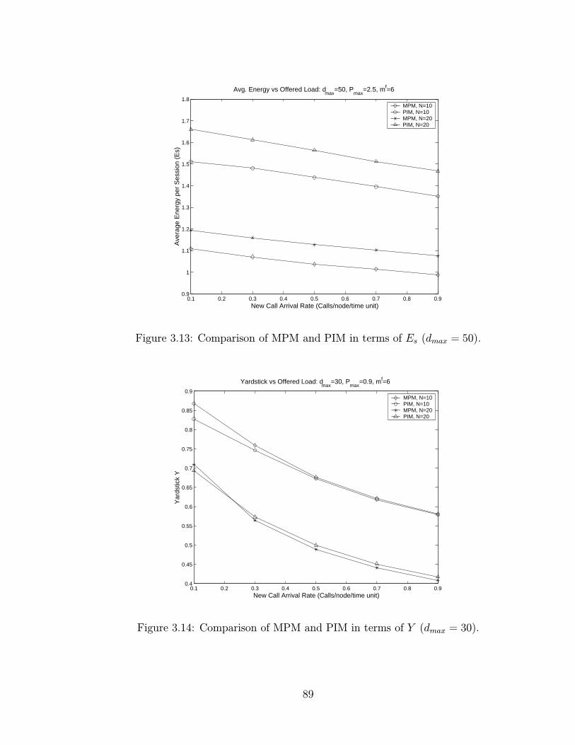
0.1 0.2 0.3 0.4 0.5 0.6 0.7 0.8 0.90.9
1
1.1
1.2
1.3
1.4
1.5
1.6
1.7
1.8
New Call Arrival Rate (Calls/node/time unit)
Ave
rage
Ene
rgy
per
Ses
sion
(E
s)
Avg. Energy vs Offered Load: dmax
=50, Pmax
=2.5, mf=6
MPM, N=10PIM, N=10MPM, N=20PIM, N=20
Figure 3.13: Comparison of MPM and PIM in terms of Es (dmax = 50).
0.1 0.2 0.3 0.4 0.5 0.6 0.7 0.8 0.90.4
0.45
0.5
0.55
0.6
0.65
0.7
0.75
0.8
0.85
0.9
New Call Arrival Rate (Calls/node/time unit)
Yar
dstic
k Y
Yardstick vs Offered Load: dmax
=30, Pmax
=0.9, mf=6
MPM, N=10PIM, N=10MPM, N=20PIM, N=20
Figure 3.14: Comparison of MPM and PIM in terms of Y (dmax = 30).
89
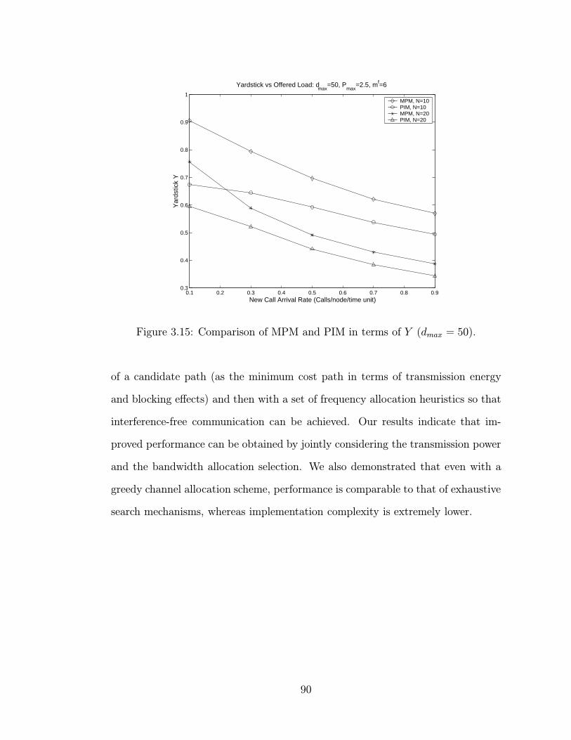
0.1 0.2 0.3 0.4 0.5 0.6 0.7 0.8 0.90.3
0.4
0.5
0.6
0.7
0.8
0.9
1
New Call Arrival Rate (Calls/node/time unit)
Yar
dstic
k Y
Yardstick vs Offered Load: dmax
=50, Pmax
=2.5, mf=6
MPM, N=10PIM, N=10MPM, N=20PIM, N=20
Figure 3.15: Comparison of MPM and PIM in terms of Y (dmax = 50).
of a candidate path (as the minimum cost path in terms of transmission energy
and blocking effects) and then with a set of frequency allocation heuristics so that
interference-free communication can be achieved. Our results indicate that im-
proved performance can be obtained by jointly considering the transmission power
and the bandwidth allocation selection. We also demonstrated that even with a
greedy channel allocation scheme, performance is comparable to that of exhaustive
search mechanisms, whereas implementation complexity is extremely lower.
90
Chapter 4
A “Blueprint” towards an Integrated Scheduling,
Access Control and Routing Scheme in Wireless
Ad-Hoc Networks
4.1 Motivation
While the Internet is evolving into a true integrated services network, wireless
data networks are becoming an integral part of the new global communication
infrastructure. In order to support a variety of applications with a wide range of
Quality-of-Service (QoS) requirements (e.g., audio and video conferencing, multi-
media information retrieval, ftp, telnet, WWW, etc.), efficient link management
and scheduling algorithms are necessary. In this chapter, we review state-of-the
art work on fair resource allocation/packet scheduling for wireline and wireless
networks and address the unique issues that arise when similar schemes must be
applied to wireless ad-hoc environments.
In wireline networks, a popular model for providing fairness and bounded de-
lay link access is the fluid fair queuing model ([15, 16]). A variety of fair queuing
91
algorithms have been proposed ([16, 17, 18]) that are based on the notion of ap-
proximating the fluid model, in which packet flows are modeled as fluids that
traverse a shared pipe. Although algorithms that follow this model perform well
in wireline networks, they do not carry over their properties to the wireless envi-
ronment. In fact, most have been shown to lose their desirable properties such as
fairness and tight delay bounds in varying capacity links. Moreover, the unique
characteristics of the wireless channel such as location-dependent and bursty errors
and location-dependent capacity often lead to situations of unfairness.
The adaptation of packet fair queuing algorithms to wireless networks has mo-
tivated a significant amount of research work [19, 20, 21, 22, 23]. Most of these
proposed algorithms are designed for a wireless cellular environment (with the
base station acting as a coordinator node) and are capable of achieving long-term
fairness by arbitrating among flows with good and bad channel error attributes
differently, and suggesting mechanisms for compensating ”lagging” flows at the
expense of ”leading” flows. However, they rely on the existence of a base station
which plays the role of the local arbitrator and thus are not appropriate for other
types of network architectures such as ad-hoc networks.
Wireless ad-hoc networks present some key characteristics that necessitate a
modified approach to the problem of fair scheduling. Channel access is not always
controlled by a central arbitrator node but has to be achieved in a distributed fash-
ion and in a way that collisions are avoided (to the degree this is feasible). At the
same time, the possibility to re-use bandwidth gives rise to the trade-off between
fair scheduling and maximum resource utilization. Most important, loading and
congestion at each node is not dependent on the scheduling discipline only but
also on routing decisions. If the routing algorithm and the metrics used to make
92
routing decisions do not adequately capture the effects of the radio link quality
and the capacity assignment by the access control and scheduling mechanisms, in-
efficient route assignments may result that could lead to increased congestion and
lost throughput. On the other hand, methods of assigning the bandwidth need to
be based on the traffic requirements at each node (based on new traffic originating
and flows being routed through the node) as well as the quality of the links from
a given node. Last, but not least, channel errors which are location-dependent
and bursty in nature may affect flows selectively. Therefore, mechanisms to com-
pensate for nodes and flows that experience poor channel quality must be part of
every scheduling discipline.
Based on these remarks, we argue upon the fact that the design of efficient
protocols for wireless multi-hop networks must address the dependencies between
routing, access control and scheduling, and radio link functions. We propose a
preliminary unified scheme which performs node-level access control (also called
node-level scheduling), flow-level scheduling and route assignment in a hierarchi-
cal framework with interactions among the three protocol solutions. Our approach
can be regarded as a ”blueprint” towards the future development of more detailed
unified solutions. The variety and the complexity of issues that arise due to the
numerous trade-offs involved in such a design will become apparent as we discuss
our methodology in the following sections. However, even with a simplified pre-
liminary performance evaluation, useful conclusions on the interdependencies of
our protocols are drawn that reveal the potential and the possibilities that exist
towards these directions.
The rest of the chapter is organized as follows. In the next section we review
a class of scheduling disciplines, used for scheduling best-effort traffic in wire-line
93
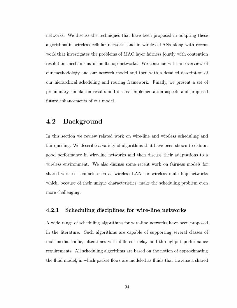
networks. We discuss the techniques that have been proposed in adapting these
algorithms in wireless cellular networks and in wireless LANs along with recent
work that investigates the problems of MAC layer fairness jointly with contention
resolution mechanisms in multi-hop networks. We continue with an overview of
our methodology and our network model and then with a detailed description of
our hierarchical scheduling and routing framework. Finally, we present a set of
preliminary simulation results and discuss implementation aspects and proposed
future enhancements of our model.
4.2 Background
In this section we review related work on wire-line and wireless scheduling and
fair queuing. We describe a variety of algorithms that have been shown to exhibit
good performance in wire-line networks and then discuss their adaptations to a
wireless environment. We also discuss some recent work on fairness models for
shared wireless channels such as wireless LANs or wireless multi-hop networks
which, because of their unique characteristics, make the scheduling problem even
more challenging.
4.2.1 Scheduling disciplines for wire-line networks
A wide range of scheduling algorithms for wire-line networks have been proposed
in the literature. Such algorithms are capable of supporting several classes of
multimedia traffic, oftentimes with different delay and throughput performance
requirements. All scheduling algorithms are based on the notion of approximating
the fluid model, in which packet flows are modeled as fluids that traverse a shared
94
����
����
����
flow 1
flow 2
flow n
output link
Figure 4.1: A node with several flows sharing a common channel
pipe. Consider for example the system shown in figure 4.1, where packets from
several flows are stored in different queues of the same node before being trans-
mitted to an output link. A fair scheduling algorithm is required for determining
which flow to serve at every time so that a set of fairness criteria are satisfied. We
describe the most fundamental of these schedulers and discuss their main principles
of operation.
Generalized Processor Sharing (GPS)
The fair queuing algorithms proposed in the literature attempt to approximate
the Generalized Processor Sharing discipline proposed in [15]. GPS is an ideal
scheduling discipline that visits each nonempty queue in turn and serves an in-
finitesimally small amount of data, so that in any finite time interval, it can visit
each logical queue at least once. Moreover, connections can be associated with ser-
vice weights and receive service in proportion to their weights whenever they have
data in their queue. However, GPS is not implementable because it is supposed
to serve an infinitesimal amount from each nonempty queue. In actual systems,
packets must be transmitted as a whole and this has motivated research in the
area of packet fair queuing algorithms.
95

Round-Robin and Weighted Round-Robin (WRR)
The simplest emulation of GPS is a round-robin scheduler which serves one
packet from each non-empty logical queue instead of an infinitesimal amount. If
connections have different weights, a Weighted Round-Robin scheduler serves a
connection in proportion to its weight. However, WRR approximates GPS rea-
sonably well only if all packets have the same size. If packets have different sizes,
the WRR scheduler divides each connection’s weight by its mean packet size to
normalize the weights. In some situations, a server may not know in advance the
mean packet size of a connection (for example in the case of compressed video
transmission) and then WRR cannot allocate bandwidth in a fair way. Another
problem is that WRR is unfair over short time scales (some connections may get
more service than others in one round-time) and if a connection has a small weight
or if the number of connections is large, this may lead to long periods of unfairness.
Deficit Round-Robin (DRR)
Deficit Round-Robin [18] is a modification to WRR so that it can handle vari-
able packet sizes without knowledge of the mean packet size of each connection in
advance. In DRR implementation, each back-logged connection is associated with
a deficit counter which is initially set to zero. The scheduler visits each back-logged
connection in turn and tries to serve one quantum worth of bits from it. The only
difference from the traditional round-robin is that if a queue is not able to send
a packet in a previous round because its packet size was too large, the remainder
from the previous quantum is added to the quantum for the next round. Thereby,
queues that were short-changed in a round are compensated in the next round.
Weighted Fair Queuing (WFQ)
In Weighted Fair Queuing [16] (also referred to as Packet-by-Packet GPS [15])
96
packets are served in order of their service tags which are computed by simulating
a hypothetical GPS on the side. Since packets must be served as a whole (and
not a bit at a time), WFQ computes the start tag and then the finish tag of every
new packet, the latter being the time the packet would have completed service if
a GPS server was being used. Packets are then served in order of their finish tags.
The finish tag computation depends on a variable called the round number, which
increases at a rate inversely proportional to the number of active connections. In
particular, if pjf and ljf denote the jth packet of flow f and its length, respectively,
and if A(pjf ) denotes the arrival time of packet pjf at node i, then the start tag
S(pjf) and finish tag F (pjf) of packet pjf are defined as:
S(pjf) = max{v[A(pjf)], F (pj−1f )}, j ≥ 1 (4.1)
F (pjf) = S(pjf) +ljfφj
(4.2)
where F (pof) = 0 and v(t) is defined as:
dv(t)
dt=
C∑j∈B(t) φj
(4.3)
where C is the capacity of the server, B(t) is the set of back-logged flows at time
t in the bit-by-bit round-robin server and φj is the weight associated with flow j.
WFQ then schedules packets in the increasing order of their finish tags.
Although WFQ achieves fairness comparable to GPS, it is complex (in terms
of implementation) because it needs to maintain per connection scheduler state
which may be expensive for schedulers that serve large numbers of connections.
Moreover, as it is demonstrated in [24], the computation of v(t) requires simulation
of a bit-by-bit round-robin server in real time which may in turn require processing
97
of O(Q) events per packet transmission, where Q is the number of active queues.
With the current definition of virtual time though, it has been shown in [17] that
WFQ becomes unfair over variable rate servers and hence is not a reliable option.
Start-Time Fair Queuing (SFQ)
The Start-time Fair Queuing algorithm proposed in [17] overcomes some of the
deficiencies of WFQ. It differs from WFQ in that packets are scheduled in order of
their start-tags (computed by equation 4.1) instead of the finish-tags. Furthermore,
v(t) is defined as the start tag of the packet in service at time t. As is evident
from this definition, the computation of v(t) is inexpensive (in fact complexity is
O(logQ) per packet where Q is the number of flows at the server). In addition to
that, SFQ has been shown to retain fairness even when the capacity of the link is
variable. However, the delay properties of SFQ for high throughput applications
are not as good as those for the WFQ algorithm; it outperforms WFQ though for
low throughput applications.
4.2.2 Scheduling disciplines for cellular wireless networks
Scheduling algorithms that work well in wire-line networks do not always carry
over to the wireless environment and in most situations they have been known to
lose their desirable properties, such as fairness and tight delay bounds. Part of this
behavior is attributed to the following three characteristics of the wireless channel:
– capacity is severely limited and time varying
– channel errors are location-dependent and bursty in nature
– need for channel access control mechanisms in shared medium configurations.
98
Although the problem of varying capacity channels is partially addressed by use
of SFQ schedulers, the problem of location- dependent and bursty channel errors
may lead to undesirable situations. For example, sessions that experience errors
may receive significantly less service than what they would be entitled to, whereas
sessions that have access to error-free channels take advantage. In order to ac-
count for channel errors, wireless scheduling algorithms usually adapt a wire-line
scheduling algorithm to the situation where flow specific errors are present. This
means that wireless scheduling algorithms differentiate between flows experiencing
channel errors from those with a clean channel. Each flow is labeled as being lead-
ing, lagging or in sync depending on whether its actual received service is ahead
of, behind of, or in accordance to its error-free service which it would have received
if a clean-channel was available all the time. Typically, flows that are scheduled
and are experiencing channel errors are taken offline (and hence are considered
as lagging) and the scheduler instead may choose to allocate the excess capacity
to flows with clean wireless channels (resulting in their service leading the ideal
service).
Different wireless algorithms choose to address the issue of lag and lead in
different ways. In addition, almost all wireless algorithms require an estimate of
the per flow channel characteristics (error, capacity). Since any estimate is prone
to error, given the random nature of a wireless channel, wireless scheduling and
admission control algorithms will under-perform the ideal wire-line scheduler when
channel errors reduce per flow capacity. In order to compensate for the ambigu-
ity and error in capacity estimates, wireless algorithms must have compensatory
mechanisms such as the lag/lead compensation system or a method where buffer
capacity is always reserved to help accommodate flows with poor channel quality.
99
A brief summary of the main wireless scheduling algorithms is given below:
– Channel State Dependent Packet Scheduling (CSDPS), in [21]: A weighted
round-robin (WRR) scheduling discipline is used to schedule flows which
are error free. There is no lag/lead measurement for flows and hence no
compensation. Implementation complexity is low.
– Idealized Wireless Fair Queuing (IWFQ), in [19]: WFQ is used for error free
service. The lag is upper bounded and the scheduler maintains lag and lead
for each flow and favors lagging flows by allowing them to capture the channel
as soon as they perceive error free channels. This algorithm has poor short
term fairness properties and throughput bounds while long term fairness and
bounds are provided.
– Wireless Packet Scheduling (WPS), in [19]: A modified version of WRR
is used where the bandwidth allocation is as per the weights, but spread
out rather than continuous. The algorithm maintain lag and lead measures
and compensates for lags in two ways: changing weights of lagging flows in
subsequent frames, or exchanging slots between error prone and error free
flows in the same frame. The performance is similar to IWFQ.
– Channel Condition Independent Fair Queuing (CIF-Q), in [22]: STFQ is the
error free service model. Lags and leads are computed and lagging flows are
compensated only when leading flows relinquish slots. CIF-Q has the best
short term and long term fairness and throughput properties though lagging
flows may suffer poor short term fairness.
– Enhanced Class Based Queuing with Channel State Dependent Packet Schedul-
ing, in [25]: This model combines the CSDPS scheduling with Class based
100

Queuing. Lag/lead compensation is similar to IWFQ.
– Wireless Fair Service (WFS), in [23]: An enhanced version of WFQ is used
for error free service. Lead and lag are bounded for each flow. A leading flow
with a lead l and a lead bound lmax relinquishes 1lmax
slots. WFS is shown
to achieve the tightest short term fairness and throughput bounds among all
algorithms. It also provides good long term performance. Lag compensation
may be slow.
The idea of lag/lead compensation while temporarily subverting priorities and
fairness provides ways of compensating for errors which are flow specific. Note that
lag and lead bounds can be used to control the extent to which this mechanism
actually redistributes bandwidth among lagging and leading flows.
4.2.3 Scheduling in wireless LANs
None of the scheduling algorithms listed above addresses explicitly the problem
of channel access in a distributed topology. In all situations it is assumed that a
central coordinator node exists (e.g. a base station) which performs the scheduling
functions and allocates bandwidth to the contending uplink flows. Early work in
medium access control (MAC) protocols for wireless LANs has focused on provid-
ing fully distributed schemes for channel access. Protocols such as MACA [26]
and MACAW [27] were based on Request-to-Send (RTS), Clear-to-Send (CTS)
packet exchange and binary exponential back-off mechanisms to mitigate collision
effects. They were limited though in that they attempted to provide equal share
of bandwidth to different nodes, without differentiating among classes of service
with different bandwidth requirements and without taking into account channel
101

errors. In a later work [28], Vaidya et. al. proposed a distributed fair scheduling
algorithm motivated by the collision avoidance mechanisms of the IEEE 802.11
standard for wireless LANs. Their work suggests an emulation of start-time fair
queuing in a distributed manner, by modifying the back-off interval mechanism,
so that nodes ready to transmit packets with smaller tags have smaller back-off
intervals. Even though in the performance evaluation location dependent channel
errors were considered, there was no explicit mechanism on how to react or take
into account poor quality link situations.
4.2.4 Scheduling in wireless multi-hop networks
Most of the features encountered in a wireless LAN environment are also present
in wireless multi-hop networks. In fact, a single logical channel is again shared
among many contending users and there is lack of global knowledge of the traf-
fic flows in each node, since information is distributed. However, in multi-hop
wireless networks, spatial reuse of the channel bandwidth is possible and thereby
there is an inherent trade-off between achieving fairness among contending flows
and at the same time maximizing channel utilization. In [29] a model is presented
that addresses this trade-off. A centralized algorithm is first proposed that pro-
vides a minimum fair allocation of bandwidth for each packet flow and attempts
to maximize spatial bandwidth reuse. A distributed implementation is then dis-
cussed based on a back-off channel contention scheme. Some relevant work is also
presented in [30], where only the fairness problem is studied without taking into
account channel utilization issues. This work focuses mostly on the MAC-layer
aspects of the problem and on developing contention resolution algorithms that
execute independently at each node and are translated into a sophisticated back-
102
off algorithm for achieving proportional fairness.
Although both [29] and [30] present some novel features on how to model
fairness in a multi-hop network architecture, their focus remains on the implemen-
tation issues of contention resolution mechanisms in a distributed fashion. The
effects of channel errors which, as was discussed earlier, constitute a significant
hurdle in achieving fairness in wireless environments are not directly addressed.
Moreover none of these studies, and no other study that we know of, considers
the dependencies between scheduling algorithms and route assignments. Methods
of assigning the bandwidth however, need to be based on the traffic requirements
at each node as well as routing information and vice-versa. With this in mind,
we propose in the next section a hierarchical scheduling scheme and a method of
addressing the dependencies between capacity allocation and route assignments.
4.3 A unified approach to scheduling, access-control
and routing in ad-hoc networks
4.3.1 Overview
We propose a hierarchical scheme that considers a wireless channel shared by
multiple nodes. Capacity allocation is made at the node-level and the flow level
based on link and flow-level error characteristics and the routing assignments. The
routing algorithm is shortest-path based with the link-distance metrics calculated
based on congestion information and the current node and flow-level schedules.
A two-tier scheduling mechanism is proposed, namely node-level and flow-level
scheduling. Each node is associated with an adaptive metric/weight which is up-
103
dated periodically and is a function of the traffic requirements at the node (based
on new traffic originating and flows being routed through the node) as well as the
quality of the links from a given node (captured by number of lost packets due to
channel errors). Once all the nodes have determined their bandwidth allocations,
they schedule their flows individually using a similar mechanism with the differ-
ence that the metrics are now per-flow and depend on the traffic requirements and
lost throughput of individual flows. With this multi-level approach we can han-
dle errors that are flow-selective in nature and compensate flows that are lagging
because they have been experiencing poor quality channels.
In order to address the dependencies between routing and scheduling, the rout-
ing assignments should be updated periodically. The concept of least-resistance
routing (LRR), described in [31], can be used to determine link-distance metrics
that depend on the link-quality. By updating the route assignments, flows that
have been experiencing poor links due to location-dependent errors have the chance
of re-negotiating their paths. Note that a flow is defined by its source-destination
pair and therefore even if a link in the routing path suffers the whole flow will be
affected. On the other hand, node-level and flow-level schedules always adapt to
the most current routing vectors since they are determined as functions of the new
traffic requirements.
4.3.2 Proposed model
We consider an ad-hoc network where nodes are organized into a number of over-
lapping clusters. Nodes that belong to the same cluster are connected with each
other via direct links. For example, in the network of figure 4.2, nodes A,B and
E belong to the same cluster; nodes B,C and D belong to a different cluster.
104
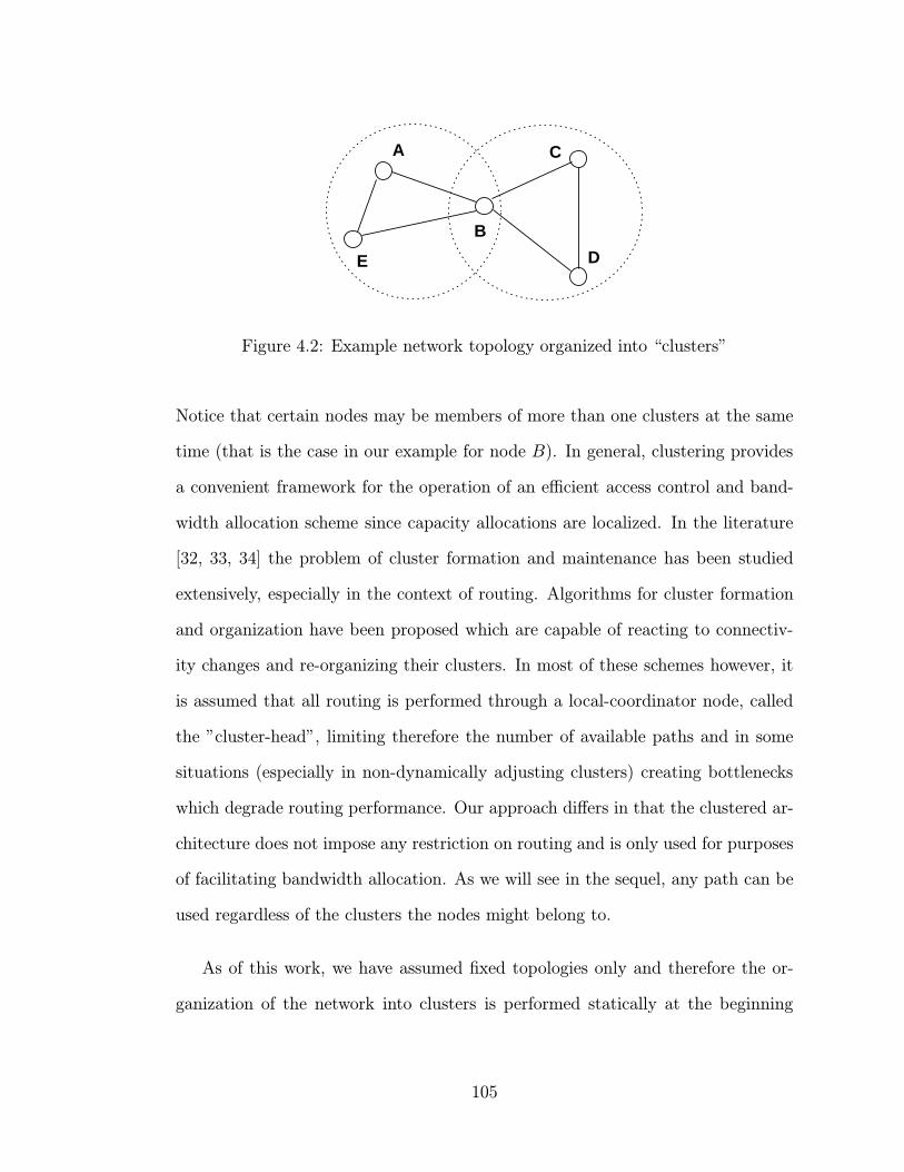
A
E
B
C
D
Figure 4.2: Example network topology organized into “clusters”
Notice that certain nodes may be members of more than one clusters at the same
time (that is the case in our example for node B). In general, clustering provides
a convenient framework for the operation of an efficient access control and band-
width allocation scheme since capacity allocations are localized. In the literature
[32, 33, 34] the problem of cluster formation and maintenance has been studied
extensively, especially in the context of routing. Algorithms for cluster formation
and organization have been proposed which are capable of reacting to connectiv-
ity changes and re-organizing their clusters. In most of these schemes however, it
is assumed that all routing is performed through a local-coordinator node, called
the ”cluster-head”, limiting therefore the number of available paths and in some
situations (especially in non-dynamically adjusting clusters) creating bottlenecks
which degrade routing performance. Our approach differs in that the clustered ar-
chitecture does not impose any restriction on routing and is only used for purposes
of facilitating bandwidth allocation. As we will see in the sequel, any path can be
used regardless of the clusters the nodes might belong to.
As of this work, we have assumed fixed topologies only and therefore the or-
ganization of the network into clusters is performed statically at the beginning
105
of network operation. Dynamic topologies necessitate the use of sophisticated
clustering algorithms that react to topological changes by adjusting the cluster-
memberships and dependencies and are beyond the scope and objectives of this
study.
Nodes do not need to maintain global knowledge of the network parameters;
instead, they rely on selected information that is exchanged periodically among
members of a cluster to determine their weights and make the scheduling decisions
in a distributed fashion. The operational environment consists of shared radio links
with nodes operating in half duplex mode: they can either transmit or receive but
not both simultaneously. Nodes belonging to more than one clusters can receive
packets from only a single node in each cluster but not from multiple clusters
simultaneously. For example, in the topology shown in figure 4.2, node B can
receive packets from nodes A and C, but not from C and D in the same time
slot. Multiple packet receptions from different clusters may be possible if nodes
use directional/smart antennas, have multiple receiver elements and if the clusters
are organized to isolate interference.
Time is slotted and slots are grouped into fixed length frames. We assume
a single packet can be transmitted per slot. Allocations of slots to nodes and
flows, and route selection of the flows can only be performed at the beginning of a
frame. Since our focus is on the bandwidth sharing principles rather than on the
implementation details of the MAC-layer protocol, we assume that every node’s
allocated slots get assigned to the appropriate portion of each time-frame by a
mechanism that is not the purpose of this study. Nonetheless, the development of
a MAC-layer protocol that implements our scheme can be performed at a future
time.
106
Under these considerations, the approach to solving the node access, flow
scheduling and routing problem jointly evolves as an iterative procedure between
the following three steps:
Step 1. Node-level scheduling: Determine the capacity allocation to each node
in the cluster based on a weighted round-robin scheme using fixed routing
assignments for all flows in each node.
Step 2. Flow-level scheduling: Determine the capacity allocation to each flow
in the node based on a weighted round-robin scheme using fixed routing
assignments for all flows in that node.
Step 3. Route-updates: Determine the routes of the flows at each node: i.e., for
all the flows in a particular node determine which of the nearest neighbors
the flow must be directed to.
4.3.3 Link error adjusted rate (LEAR) measure
The node and flow-level scheduling is performed by a modified weighted round-
robin algorithm in which the nodes and their serviced flows determine their weights
in proportion to a measure called the link error adjusted rate (LEAR).
Nodes are aware of the number of packets buffered for transmission at the
beginning of every frame. Moreover, each node estimates the channel quality
on each of its flows in terms of loss in throughput (ie. number of packets lost per
frame). Assume for example that node C in figure 4.2 has packets to be transmitted
to both B and D. Node C estimates loss in capacity due to channel errors for the
flows directed to B and to D. A link error adjusted rate (LEAR) required by node
107
C is then computed by adding the average error free service rates required by all
flows plus the lost throughput of all its links weighted in the proportion of flows
directed to that destination. In particular, for this example, if Xt(CD) represents
the number of packets waiting to be transmitted from C to D at the beginning of
frame t and Yt−1(CD) represents the lost packets for frame (t− 1) on link C to D
and similarly Xt(CB) are the packets to be transmitted from C to B and Yt(CB)
are the lost packets on link C to B, the LEAR value is computed as follows:
LEARt(C) = Xt(CB) +Xt(CD) +
Yt−1(CD)×Xt(CD)
Xt(CD) +Xt(CB)+ Yt−1(CB)×
Xt(CB)
Xt(CB) +Xt(CD)
(4.4)
The weights of the WRR scheduler are then determined in proportion to the
LEAR values of each node rather than the average rate required. The two vari-
ables X and Y capture two different effects. While X models the congestion level
at each node, Y estimates the link quality between a node and its neighbors. As
congestion increases in a node, the values of the X variable increase and the node
demands a higher share of the bandwidth. Also, the LEAR value increases as
Y increases or the link quality decreases. The node thus tries to compensate for
lost throughput by using higher bandwidth. This appears to be inefficient since
nodes with poor quality links might hog bandwidth and throughput is lost. This
is prevented though if the link metrics for the routing mechanisms are selected
carefully to discourage use of links with poor quality and excessive delays. Also, as
the queues in neighboring nodes increase, their X values increase and they obtain
more bandwidth preventing starvation. This is a method for lag-lead compen-
sation, as flows which are lagging have higher values of the LEAR measure and
108
obtain higher bandwidth.
4.3.4 Routing updates
In the determination of the node and flow capacity allocations, the route assign-
ments are fixed, i.e. each node knows the immediate next-hop neighbor for each
flow. At the beginning of each time frame, routes may be recomputed based on the
current schedules, and used in the subsequent time frame. In order to determine
the route for each flow, we associate each link with an adaptive distance-metric
(cost of transmitting over that link) and use a distributed version of Bellman-Ford
[12] algorithm for shortest-path computation. Link metrics should be selected in a
way that preference is given to neighboring nodes with lower congestion (smaller
aggregate queue size) and links with lower estimated service time. The metric we
propose is proportional to an estimate of the average packet delay, which can be
obtained if a packet is stamped when buffered at node so that upon departure
its delay can be computed. More sophisticated metrics that may capture link
congestion can be plugged in without having to modify the algorithm.
An appropriate update interval must be determined for periodically re-computing
the link metrics and adjusting the route assignments. In practice, it cannot hap-
pen at the beginning of every frame, for the following reasons. First, the overhead
of updating the link metrics, running the shortest-path algorithm and adjusting
all the routing tables is too large. Second, if the routing tables are updated very
frequently, oscillations may occur, affecting the great majority of packets that
will have to travel along “loops” before reaching their intended destinations. The
problem of determining a good update interval is re-visited in the performance
analysis where we run experiments for a range of different intervals and examine
109
their effects on performance.
4.4 Description of algorithms
4.4.1 Notation
As was mentioned above, nodes are organized into clusters as in the example shown
in figure 4.2 and each node may handle multiple traffic flows each of which has a
specific source and destination. Note here that we define a flow from end-to-end
unlike other schemes where a flow denotes a transmitter-receiver pair. We shall
use the following notation:
• Xt(i): total number of packets waiting for transmission at node i at the
beginning of frame t.
• Xt(i, j): total number of packets waiting to be transmitted from node i to
node j at the beginning of frame t.
• Xft (i, j): total number of packets from flow f waiting to be transmitted from
node i to node j at the beginning of frame t.
• Yt(i, j): lost throughput (packets/frame) from node i to j during frame t,
due to channel errors.
• Y ft (i, j): lost throughput (packets/frame) of flow f from node i to j during
frame t, due to channel errors.
• Nt(i): set of neighbors of node i
• Rt(i, f): neighbor receiving flow f from node i.
110
• C: number of slots per frame.
4.4.2 Node-level scheduling
Node-level scheduling refers to the access control mechanism of nodes sharing the
radio link in the same cluster. At the beginning of every frame, and in order to
determine their slot allocations, these nodes compute their LEAR measures based
on the following equation:
LEARt(i) =∑
j∈Nt(i)
Xt(i, j) +∑
j∈Nt(i)
Yt−1(i, j)×X(i, j)∑
k∈Nt(i)X(i, k)
(4.5)
Each node then calculates its weight as the ratio of its LEAR to the sum of the
LEARs of all the nodes belonging to the same cluster:
W (i) =LEARt(i)∑
j∈cluster LEARt(j)(4.6)
The capacity allocation Ct(i) of node i is then given by:
Ct(i) = bC ×W (i)c (4.7)
Since the sum of the Ct(i) may be less than the frame capacity C and in order not
to waste slots, each node i maintains a deficit weight Wd(i) equal to:
Wd(i) = C ×W (i)− Ct(i) (4.8)
Clearly the number of unused slots will be less than the number of nodes in the
cluster. If these excess slots are equal to m, then they will be allocated to the nodes
with the m larger values of Wd(i). The notion of the deficit weight is similar to the
way the deficit round-robin works (described in section 4.2) and is utilized because
packets must be transmitted as a whole, but no slots should remain unused.
111

Nodes that belong to multiple overlapping clusters need to perform an extra
step. These nodes (for example node B in figure 4.2) will end up with more
than one allocations from the above scheme, namely one for each cluster they
are members of. To resolve this conflict, they choose as their final allocation
that with the minimum number of slots. For example, if node i is a member
of n different clusters, then it will come up with n different allocations, denoted
by Ct,l(i), l = 1, · · · , n. According to our proposed ”tie-breaker” rule, the final
allocation will be given by:
Ct(i) = min1≤l≤nCt,l(i) (4.9)
The tie-breaker rule in a sense guarantees that the aggregate number of slots
allocated to the nodes of a single cluster never exceeds the size of a single frame.
On the other hand, it may result in wasting some bandwidth in clusters where the
”common” node was entitled to additional slots that it had to give up. This can
be avoided by modifying the algorithm to proceed to a second round of scheduling
where the unused slots are re-negotiated between the rest of the nodes in the
cluster.
4.4.3 Flow-level scheduling
Once the node-level scheduling is complete, nodes must arbitrate among multiple
flows they are serving. The task of the flow level scheduling mechanism is to divide
the allocated bandwidth Ct(i) of node i among its contending flows. We are using
LEAR-based measures again, this time for determining the weights of the flows,
similarly as we did in the previous section for the nodes. The LEAR measure of
112
flow f at node i is computed based on the following formula:
LEAR(i, f) = Xft (i, R(i, f)) + Y f
t−1(i, R(i, f))×Xft (i, R(i, f))∑
kXkt (i, R(i, k))
(4.10)
The individual flow weights can be obtained by dividing each flow’s LEAR measure
with the sum of the LEARs of one node’s flows:
W (i, f) =LEARt(i, f)∑
k∈ flow in node i LEARt(i, k)(4.11)
The capacity allocation of flow f is then given by
Cft (i) = bCt(i)×W (i, f)c (4.12)
Once again, as the sum of the Cft (i) may be less than the node’s allocated capacity
Ct each flow f maintains a deficit weight Wd(i, f) equal to:
Wd(i, f) = Ct(i)×W (i, f)− Cft (i) (4.13)
and the excess slots are again allocated to the flows with the larger values of deficit
weights Wd(i, f).
4.4.4 Routing
Routing is based on the periodic execution of the shortest-path computation al-
gorithm; in particular a distributed version of Bellman-Ford [12] algorithm is em-
ployed. Each link is associated with an adaptive distance metric (the cost of using
a particular link) which is updated periodically. The update interval (UI) is a
parameter of the algorithm and indicates how often (in number of frames) the link
metrics must be updated and the Bellman-Ford must be executed so that rout-
ing assignments are revised. The link distance-metrics are direct estimates of the
average delay per packet transmitted over each link.
113
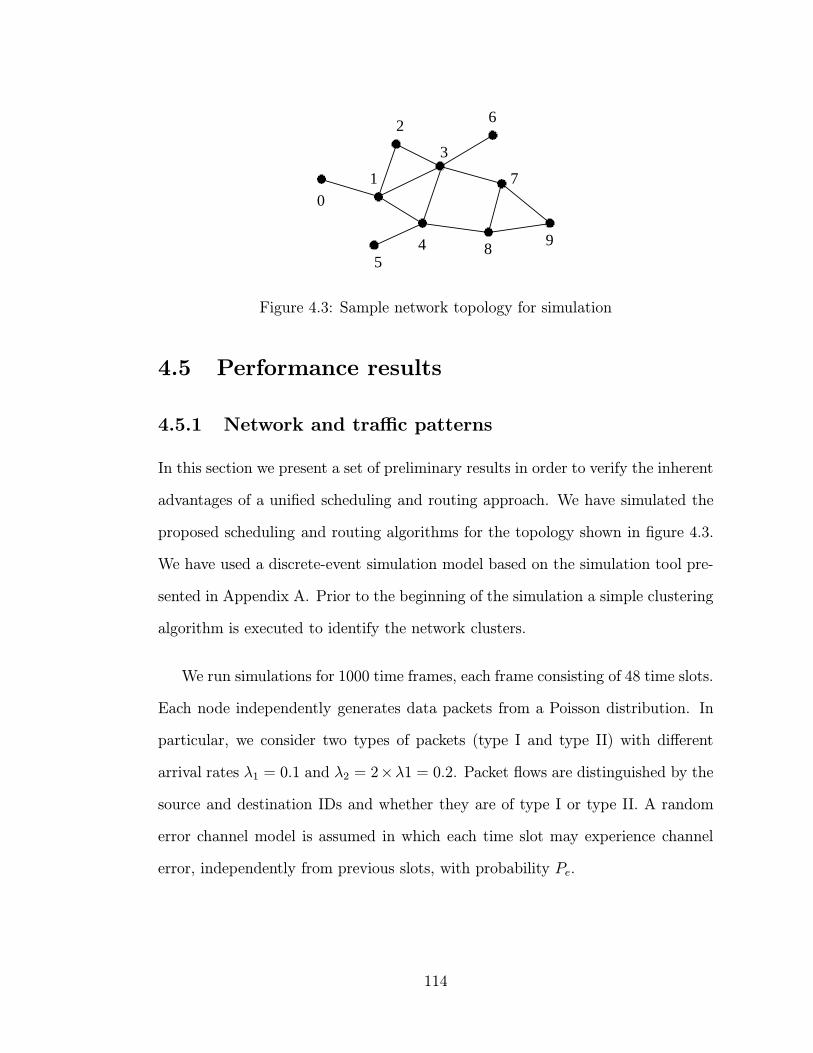
������
������
���
���
��������
������
������
����
�������� ��
������
����
������
������
��������
01
2
3
6
54 8 9
7
Figure 4.3: Sample network topology for simulation
4.5 Performance results
4.5.1 Network and traffic patterns
In this section we present a set of preliminary results in order to verify the inherent
advantages of a unified scheduling and routing approach. We have simulated the
proposed scheduling and routing algorithms for the topology shown in figure 4.3.
We have used a discrete-event simulation model based on the simulation tool pre-
sented in Appendix A. Prior to the beginning of the simulation a simple clustering
algorithm is executed to identify the network clusters.
We run simulations for 1000 time frames, each frame consisting of 48 time slots.
Each node independently generates data packets from a Poisson distribution. In
particular, we consider two types of packets (type I and type II) with different
arrival rates λ1 = 0.1 and λ2 = 2×λ1 = 0.2. Packet flows are distinguished by the
source and destination IDs and whether they are of type I or type II. A random
error channel model is assumed in which each time slot may experience channel
error, independently from previous slots, with probability Pe.
114
4.5.2 Performance measures
Performance is measured in terms of average throughput (TP ) and average packet
delay D. Average throughput is computed as the percentage of generated packets
delivered to their destinations during the simulation time. Average packet delay
is the average time spent by all packets in the network. Note though, that for
those packets delivered to the destination, the delay contribution is the complete
end-to-end delay, whereas for packets not reaching the destination, the contribu-
tion is the amount of time from generation to the end of the simulation. Although
this contribution may negatively bias the results as these packets never reach the
destination, it is included since they contribute to the delay and the ratio of un-
delivered to delivered packets is not always negligible. For each packet received
by the intended destination we calculate the packet delay and use it towards the
computation of average packet delay. For each flow we calculate the number of
delivered and undelivered packets and use them towards the calculation of the
average throughput.
4.5.3 Simulation results
Tables 4.1 and 4.2 summarize performance results for the cases of “slot-error”
rates of Pe = 0.1 and Pe = 0.2 respectively. The first column of each table lists
the values of the update interval (UI) (the period, in number of frame, that we
adjust the routing assignments). The last row F corresponds to the case of static
routing, where the routing assignments did not change during the simulation. The
average packet delays are normalized with respect to the minimum value obtained
for each table.
115
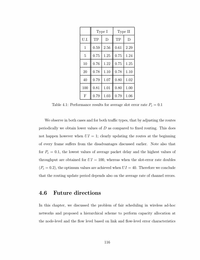
Type I Type II
U.I. TP D TP D
1 0.59 2.56 0.61 2.29
5 0.75 1.25 0.75 1.24
10 0.76 1.22 0.75 1.25
20 0.78 1.10 0.78 1.10
40 0.79 1.07 0.80 1.02
100 0.81 1.01 0.80 1.00
F 0.79 1.03 0.79 1.06
Table 4.1: Performance results for average slot error rate Pe = 0.1
We observe in both cases and for both traffic types, that by adjusting the routes
periodically we obtain lower values of D as compared to fixed routing. This does
not happen however when UI = 1; clearly updating the routes at the beginning
of every frame suffers from the disadvantages discussed earlier. Note also that
for Pe = 0.1, the lowest values of average packet delay and the highest values of
throughput are obtained for UI = 100, whereas when the slot-error rate doubles
(Pe = 0.2), the optimum values are achieved when UI = 40. Therefore we conclude
that the routing update period depends also on the average rate of channel errors.
4.6 Future directions
In this chapter, we discussed the problem of fair scheduling in wireless ad-hoc
networks and proposed a hierarchical scheme to perform capacity allocation at
the node-level and the flow level based on link and flow-level error characteristics
116
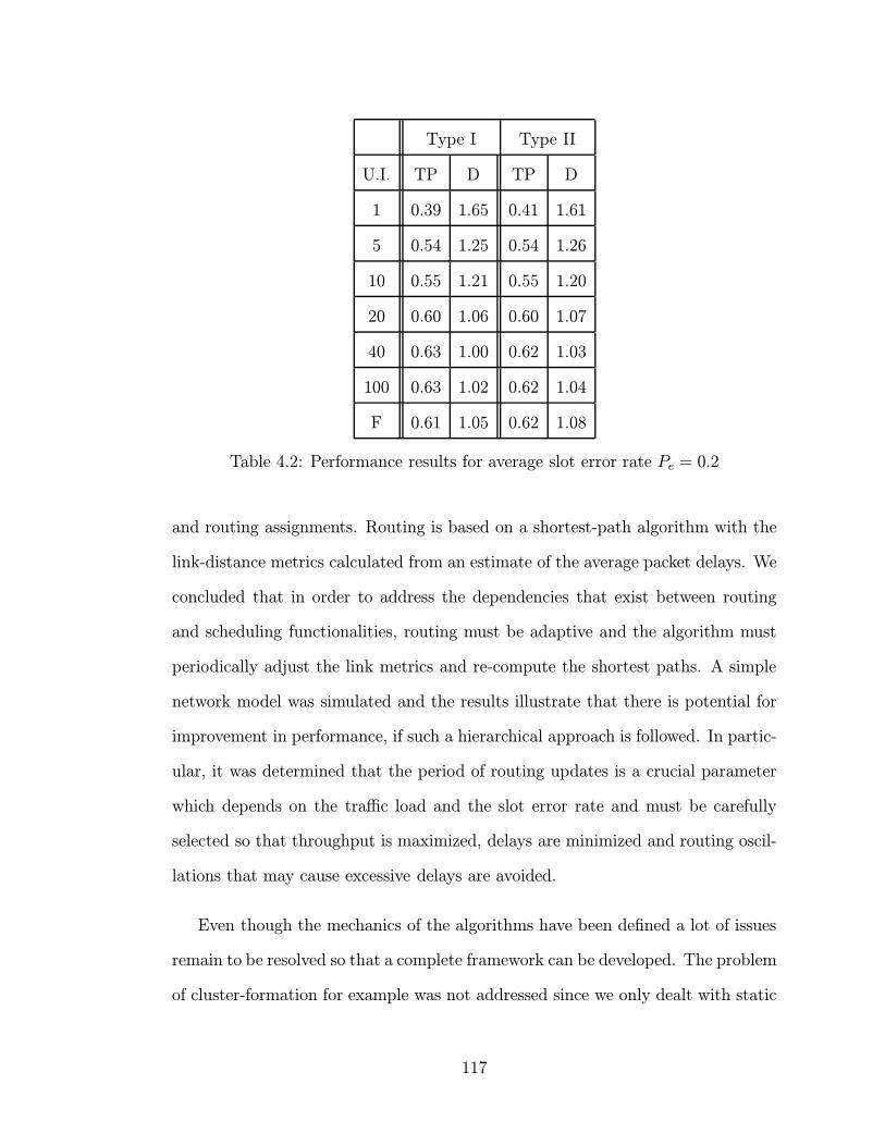
Type I Type II
U.I. TP D TP D
1 0.39 1.65 0.41 1.61
5 0.54 1.25 0.54 1.26
10 0.55 1.21 0.55 1.20
20 0.60 1.06 0.60 1.07
40 0.63 1.00 0.62 1.03
100 0.63 1.02 0.62 1.04
F 0.61 1.05 0.62 1.08
Table 4.2: Performance results for average slot error rate Pe = 0.2
and routing assignments. Routing is based on a shortest-path algorithm with the
link-distance metrics calculated from an estimate of the average packet delays. We
concluded that in order to address the dependencies that exist between routing
and scheduling functionalities, routing must be adaptive and the algorithm must
periodically adjust the link metrics and re-compute the shortest paths. A simple
network model was simulated and the results illustrate that there is potential for
improvement in performance, if such a hierarchical approach is followed. In partic-
ular, it was determined that the period of routing updates is a crucial parameter
which depends on the traffic load and the slot error rate and must be carefully
selected so that throughput is maximized, delays are minimized and routing oscil-
lations that may cause excessive delays are avoided.
Even though the mechanics of the algorithms have been defined a lot of issues
remain to be resolved so that a complete framework can be developed. The problem
of cluster-formation for example was not addressed since we only dealt with static
117

topologies. In mobile, dynamic networks however, a clustering scheme, capable of
reacting quickly to connectivity changes by reorganizing its clusters is necessary.
Furthermore, it would be interesting to examine the performance for a variety of
channel error models (bursty, location-dependent, etc.) and for different types of
traffic (variable rates).
118
Chapter 5
Conclusions
We have studied a set of different problems that arise in the context of wireless
ad-hoc networks. Our focus was on identifying issues related to several unique
characteristics of multi-hop networks and on proposing solutions in the context of
network control. In particular, we concentrated on problems related to the need for
energy and bandwidth- efficient operation and a class of algorithms were proposed
for achieving routing and bandwidth allocation of session-oriented traffic. The
algorithms were evaluated through extensive simulations, using a simulation tool
developed for the purposes of this study.
During the performance analysis, the existing trade-off between energy con-
sumption and blocking probability became apparent. We were also able to convert
session routing to link metric based, even though algorithms based on minimum
distance paths are normally intended for packet-switched networks. Another key
element was the monitoring of processing power and its effects to the overall energy
consumptions. Other studies have been considering this quantity as negligible but
our simulations indicated that its effects are quite important. Additional conclu-
sions were drawn on the effects of node density and network size on performance
119

and on how to extend the network lifetime by carefully choosing link metrics that
average energy expenditures over the whole set of network nodes.
The next step was a study of the problem of energy efficient routing under lim-
ited frequency resources, where we concluded that a two-step approach is most ap-
propriate. A minimum-cost candidate path is first determined and an interference-
free channel assignment is then searched. We proposed a set of heuristics for
achieving channel allocation and our results showed that even a simple greedy
heuristic, which has the advantage of ease of implementation and low complexity,
can achieve performance which is not significantly worse than exhaustive search
mechanisms. Another key point in this problem was the selection of an appro-
priate metric for determining the minimum cost path. We concluded that such a
metric has to combine information on the power requirements as well as a term
that indicates the number of blocked frequency channels by every transmission.
Last, we looked into the problem of fair scheduling and access control in wireless
multi-hop networks carrying packet-switched traffic. Our focus was on addressing
the dependencies between a two-level hierarchical approach to scheduling and route
assignments. We proposed an adaptive scheme that iterates between scheduling
and routing and adapts to traffic requirements, congestion and channel errors by
periodically adjusting the capacity allocation at both the node and flow-level and
the routing assignments (the latter at a different time scale). A preliminary per-
formance evaluation indicated that there are a lot of possibilities for improving
performance if a unified approach is followed.
Our studies were characterized by a tendency towards the vertical integration
of protocol layer functions. We noticed for example that improved performance
120
can be obtained by jointly considering physical layer, MAC and network layer
issues. This observation suggests that novel opportunities exist if we depart from
the traditional protocol-layer approaches and jointly address the issues that arise in
new types of network topologies with new requirements and innovative integrated
services.
Further studies on energy-efficient network control could also examine in detail
the problem of routing packet-switched traffic. In particular, a joint objective can
be defined in the context of minimizing energy and delay. Moreover, significant
amount of work has been exhibited in minimum energy wireless multicasting of
sessions, which can also be extended to datagram traffic where the concept of
minimizing delay adds a new dimension to the problem. And even though some
of the objectives may be parallel, the actual algorithms, metrics and trade-offs are
quite different.
121
Appendix A
Simulation model for energy-efficient routing
algorithms
We have developed a discrete-event simulation model for evaluating the algorithms
presented in chapters 2 and 3 of the dissertation. The programs are written in
ANSI C code and many of the simulation components have been developed from
scratch so that with minor modifications they can be reused in other simulations
(for example part of the programs were useful in the simulations of chapter 4). In
this section we provide an overview of our model, its main components and the
routines which handle the algorithmic functions.
Event scheduler
An event scheduler has been implemented that keeps a linked list of events
waiting to happen. Two types of events are considered; new call arrivals (New
Call) and call terminations (Term Call). Every event is associated with a specific
time instant t at which it is scheduled to occur and a pointer to the routines that
will be executed. During one event the scheduler may be called to schedule future
events. In particular when a New Call event occurs, the scheduler must schedule
the next arriving call for the node under consideration and if the call is admitted
122
to the system it must also schedule its termination (Term Call).
Event scheduling is performed by keeping an ordered linked list (Event List) of
future event notices. The first entry in the list represents the next earliest event
and therefore removal from the list is straightforward. Inserting a new event in the
list requires some search since the right place for the entry must be identified. Even
though this approach may not be optimal (the worst case scenario requires a full
search of the list), its implementation is simpler and for networks not exceeding a
few tens of nodes we have to maintain a New Call event per node (the next arrival)
and all the Term Call events (for the ongoing calls), hence the length of the list
does not increase in an uncontrolled way.
Simulation clock and time advancing mechanism
A global variable is maintained representing the simulated time, referred to
as the global-time. We follow an event-driven approach in which the scheduler
increments the global-time automatically to the time of the next earliest occurring
event. Thus there is no need for a unit-time approach in which the clock would be
incremented in constant time intervals.
Session representation
Each session is represented by a unique triple that consists of the source node
ID, the destination node ID and a counter that gets incremented by one for ev-
ery newly arriving session between the same source destination pair. Hence the
sessionID structure is represented as follows:
sessionID.source source node of session
sessionID.dest destination node of session
sessionID.index counter of sessions between each source-destination pair
123
Network model
The network is represented by a graph. Since the number of nodes for a simula-
tion run remains constant (ie no nodes may be added or deleted from the topology)
we declare a structure that represents a graph and consists of two entities: nodes
and arcs. Each node is a structure that consists of the appropriate identification
information (node id and location coordinates) as well as routing information that
is discussed in the next paragraph. The field arcs is a two-dimensional array repre-
senting every possible ordered pair of nodes. The value of each array element will
be either True or False depending on whether or not the two nodes are adjacent to
each other.
Node model
In addition to ID and location information that was mentioned above, each
node must maintain the following structures:
– an array of transceiver status which indicates whether a transceiver k is free or
in use; if a transceiver is in use, the corresponding sessionID along with the
incoming and outgoing links are stored in a one-dimensional array of size
equal to the number of transceivers, referred to as the connectivity table and
consisting of the following fields (each element of the array corresponds to a
unique transceiver):
connectivity-table[k].sessionID session in service
connectivity-table[k].in-node node from which session is received
connectivity-table[k].out-node node to which session is transmitted
connectivity-table[k].transceiver-status status of transceiver
– an array of frequency channel status which indicates whether a frequency channel
k is free or blocked from transmission for every potential next-hop receiver; if
124
a frequency channel is in use, information about the next-hop neighbor and
the ongoing sessionID is stored in the frequency-based routing table as follows
(each element of the array corresponds to a unique frequency channel):
routing[k].sessionID
routing[k].next-node
– information about the minimum cost path. In particular each node i main-
tains an array with the minimum cost to reach every possible destination
(node[i].min-distance[dest]) and the immediate neighbor that leads to that
destination (node[i].next-hop[dest]).
Routines
We summarize hereafter in pseudocode the routines that are used for estab-
lishing and terminating sessions over the selected routes, for both cases of limited
number of transceivers (Establish, Terminate) and limited number of frequency
channels (EstablishF, TerminateF and ClearPathF). Note that both Establish and
EstablishF routines return the total power consumed by the nodes in the path if
the call is admitted, whereas Terminate, TerminateF and ClearPath are called to
”tear-down” admitted or partially admitted sessions and do not return any value.
establish(sessionID)
{
power = 0;
tr-node = sessionID.source;
if (tr-node.min-distance[sessionID.dest] <∞)
/* ie a feasible path exists */
while(tr-node 6= sessionID.dest)
125
{
rc-node = node.next-hop[sessionID.dest];
reserve(tr-node,rc-node);
/* reserve updates the connectivity table and */
/* transceiver status */
power += power for transmission from tr-node to
rc-node;
tr-node = rc-node;
}
return(power);
}
terminate(sessionID)
{
tr-node = sessionID.source;
while((tr-node 6= sessionID.dest) AND
(∃ k s.t. tr-node.connectivity-table[k].session==sessionID))
{
rc-node = tr-node.connectivity-table[k].rc;
clear(tr-node, rc-node);
current-node = rc-node;
}
}
126
establishF(sessionID)
{
power = 0;
tr-node = sessionID.source;
if (tr-node.min-distance[sessionID.dest] <∞)
/* ie a feasible path may exist */
while(tr-node 6= sessionID.dest)
{
rc-node = node.next-hop[sessionID.dest];
if (∃k s.t. frequency channel[k] == free)
{
reserve(tr-node,rc-node,k);
/* reserve updates the frequency-based */
/* routing table */
blocking(tr-node,rc-node,k)
/* block neighboring nodes in accordance to */
/* interference model */
power += power for transmission from tr-node
to rc-node;
tr-node = rc-node;
}
else
{
clogged-node = tr-node;
clearpathF(sessionID, clogged-node)
127

power = 0;
break;
}
}
return(power)
}
terminateF(sessionID)
{
tr-node = sessionID.source;
while((tr-node 6= sessionID.dest) AND
(∃ k s.t. tr-node.routing[k].session==sessionID))
{
rc-node = tr-node.routing[k].rc;
clear(tr-node, rc-node,k);
unblocking(tr-node,rc-node,k);
tr-node = rc-node;
}
}
clearpathF(sessionID, clogged-node)
{
tr-node = sessionID.source;
128
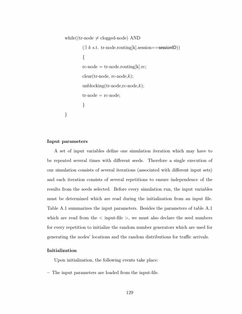
while((tr-node 6= clogged-node) AND
(∃ k s.t. tr-node.routing[k].session==sessionID))
{
rc-node = tr-node.routing[k].rc;
clear(tr-node, rc-node,k);
unblocking(tr-node,rc-node,k);
tr-node = rc-node;
}
}
Input parameters
A set of input variables define one simulation iteration which may have to
be repeated several times with different seeds. Therefore a single execution of
our simulation consists of several iterations (associated with different input sets)
and each iteration consists of several repetitions to ensure independence of the
results from the seeds selected. Before every simulation run, the input variables
must be determined which are read during the initialization from an input file.
Table A.1 summarizes the input parameters. Besides the parameters of table A.1
which are read from the < input-file >, we must also declare the seed numbers
for every repetition to initialize the random number generators which are used for
generating the nodes’ locations and the random distributions for traffic arrivals.
Initialization
Upon initialization, the following events take place:
– The input parameters are loaded from the input-file.
129

λ new call arrival rate per node per time unit
µ average call service time
metric type for minimum cost path computation
dmax maximum transmission range
max-requests cumulative number of simulated call arrivals
out-file name of file to store performance measures
preset-net set this to 0 for simulating a randomly generated network
Wp coefficient for metric M3
We coefficient for metric M3
Table A.1: Input parameters for simulation iteration
– Network graph initialization; set location of nodes and determine set of network
links based on given dmax.
– Each node schedules its first New Call event and places it in the event list.
Event reaction
As we mentioned above, we have two types of events, namely New Call and Term
Call. Both types of events result in execution of some routines upon occurence.
Depending on the assumptions (limited transceivers or limited frequencies) replace
establish and terminate with establishF and terminateF respectively.
if (event type == New Call)
{
execute Bellman-Ford for sessionID.dest
power = establish(sessionID);
130
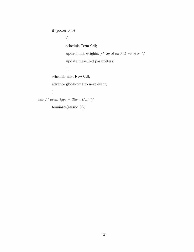
if (power > 0)
{
schedule Term Call;
update link weights; /* based on link metrics */
update measured parameters;
}
schedule next New Call;
advance global-time to next event;
}
else /* event type = Term Call */
terminate(sessionID);
131
BIBLIOGRAPHY
[1] M.S. Corson, J. Macker, and S.G. Batsell. Architectural considerations for
mobile mesh networking. In Proceedings IEEE MILCOM’96, 1996.
[2] J. E. Wieselthier, G. D. Nguyen, and A. Ephremides. Algorithms for energy-
efficient multicasting in static ad hoc wireless networks. To Appear in Mobile
Networks and Applications (MONET), 2000.
[3] J. E. Wieselthier, G. D. Nguyen, and A. Ephremides. Energy-efficient broad-
cast and multicast trees in wireless networks. To Appear in Mobile Networks
and Applications (MONET), 2000.
[4] J. E. Wieselthier, G. D. Nguyen, and A. Ephremides. Algorithms for
bandwidth-limited energy-efficient wireless broadcasting and multicasting. In
Proceedings Milcom 2000, Los Angeles, October 2000.
[5] C. Sankaran and A. Ephremides. Multicasting with multiuser detection in
ad-hoc wireless networks. In Proceedings of the 2000 International Zurich
Seminar on Broadband Communications, February 2000.
[6] V. Rodoplu and T. Meng. Minimum energy wireless networks. IEEE JSAC,
17, August 1999.
132
[7] J. H. Chang and L. Tassiulas. Routing for maximum system lifetime in wireless
ad-hoc networks. In Proceedings of the 37th Annual Allerton Conference on
Communications, Control and Computing, Monticello, IL, September 1999.
[8] J. H. Chang and L. Tassiulas. Energy conserving routing in wireless ad-hoc
networks. In Proceedings Infocom 2000, Tel-Aviv, Israel, March 2000.
[9] R. Berry, S. Finn, R. Gallager, H. Kassab, and J. Mills. Minimum energy
and delay routing in packet radio networks. In Proceedings of the 3rd Annual
FEDLAB Symposium, February 1999.
[10] A. Michail and A. Ephremides. A distributed routing algorithm for supporting
connection-oriented service in wireless networks with time-varying connectiv-
ity. In Proceedings 3rd IEEE Symposium on Computer and Communications
(ISCC 98), Athens, Greece, June 1998.
[11] A. Michail, W. Chen, and A. Ephremides. Distributed routing and resource
allocation for connection-oriented traffic in ad-hoc wireless networks. In Pro-
ceedings of the Conference on Information Sciences and Systems, Princeton,
New Jersey, March 1998.
[12] D. Bertsekas and R. Gallager. Data Networks. Prentice-Hall, 1992.
[13] A. Ephremides and T. V. Truong. Scheduling broadcasts in multihop radio
networks. IEEE Transactions on Communications, 38:456–460, 1990.
[14] I. Cidon and M. Sidi. Distributed assignement algorithms for multihop packet
radio networks. IEEE Transactions on Computing, 11:1110–1118, 1988.
133

[15] A. Parekh and R. G. Gallager. A generalized processor sharing approach
to flow control in integrated services networks. IEEE/ACM Transactions on
Networking, 1:344–357, June 1993.
[16] A. Demers, S. Keshav, and S. Shenker. Analysis and simulation of a fair queue-
ing algorithm. In Proceedings ACM SIGCOMM’89, pages 1–12, September
1989.
[17] P. Goyal, H. M. Vin, and H. Cheng. Start-time fair queueing: A schedul-
ing algorithm for integrated services packet switching networks. IEEE/ACM
Transactions on Networking, 5:690–703, 1997.
[18] M. Shreedhar and Varghese G. Efficient fair queueing using deficit round
robin. In Proceedings ACM SIGCOMM’95, pages 231–242, October 1995.
[19] S. Lu, V. Bharghavan, and R. Srikant. Fair scheduling in wireless packet
networks. In Proceedings ACM SIGCOM’97, August 1997.
[20] T. Nandagopal, S. Lu, and V. Bharghavan. A unified architecture for the
design and evaluation of wireless fair queueing algorithms. In Proceedings of
of ACM Mobicom 99, Hungary, 1999.
[21] P. Bhagwat, P. Bhattacharya, A. Krishma, and S. Tripathi. Enhancing
throughput over wireless lans using channel state dependent packet schedul-
ing. In Proceedings IEEE INFOCOM’97, April 1997.
[22] T.S. Ng, I. Stoica, and H. Zhang. Packet fair queueing algorithms for wireless
networks with location dependent errors. In Proceedings IEEE INFOCOM’98,
March 1998.
134
[23] S. Lu, T. Nandagopal, and V. Bharghavan. Fair scheduling in wireless packet
networks. In Proceedings ACM MOBICOM’98, October 1998.
[24] S. J. Golestani. A self-clocked fair queueing scheme for high speed applications.
In Proceedings INFOCOM’94, pages 636–646, April 1994.
[25] M. Srivastava, C. Fragouli, and V. Sivaraman. Controlled multimedia wireless
link sharing via enhanced class-based queueing with channel-state-dependent
packet scheduling. In Proceedings IEEE INFOCOM’98, March 1998.
[26] P. Karn. Maca - a new channel access method for packet radio. In
ARRL/CRRL Amateur Radio 9th Computer Networking Conference, Septem-
ber 1990.
[27] V. Bharghavan, A. Demers, S. Shenker, and L. Zhang. Macaw: A media
access control protocol for wireless lans. In Proceedings ACM SIGCOMM’94,
1998.
[28] N. H. Vaidya, P. Bahl, and S. Gupta. Distributed fair scheduling in a wireless
lan. In Proceedings of ACM Mobicom 2000, Boston MA, August 2000.
[29] H. Luo, S. Lu, and V. Bharghavan. A new model for packet scheduling in
multihop wireless networks. In Proceedings of ACM Mobicom 2000, Boston
MA, August 2000.
[30] T. Nandagopal, T. Kim, X. Gao, and V. Bharghavan. Achieving mac layer
fairness in wireless packet networks. In Proceedings of ACM Mobicom 2000,
Boston MA, August 2000.
135
[31] M. B. Pursley, H. B. Russel, and P.E. Staples. Routing multimedia packets
in a frequency-hop packet radio network. In Proceedings IEEE MILCOM 96,
November 1996.
[32] D.J. Baker, A. Ephremides, and J.A. Flynn. The design and simulation of
a mobile radio network with distributed control. IEEE JSAC, 2:226–237,
January 1984.
[33] P. Krishna, N. H. Vaidya, M. Chatterjee, and D. K. Pradhan. A cluster-
based approach for routing in dynamic networks. In Proceedings ACM SIG-
COMM’97, 1997.
[34] M. Gerla, J. Tzu, and C. Tsai. Multicluster, mobile, multimedia radio net-
work. Wireless Networks, 1:255–265, January 1995.
136