�������������������������

THE POSSIBILITY OF A PIGOVIAN CRASH TAX

Michael Andrews

Abstract

This paper explores the possibilities of using Pigovian taxes to internalize the costs of

automobile crashes. Automobile crashes cause significant externalities. This would seem to

provide a justification for a Pigovian tax. This paper constructs a model in which drivers

calculate costs of crashes as a fraction of their ability to pay. Under this model, Pigovian taxes

will not be able to influence behavior once a driver’s expected costs equal everything he or she

can pay.

1

�������������������������

Introduction

The act of driving creates a number of externalities. The most notable of these are

pollution, congestion, and traffic accidents.1 This paper will focus on externalities caused by

traffic accidents.2 In particular, this paper will determine under what circumstances a Pigovian

tax will align private and social accident costs.

Parry, Walls, and Harrington (2007) report that total costs of crashes, in quality-life

years, amount to $433 billion a year, or about 4.3 percent of annual GDP. The US Department of

Transportation concludes that 16,352,041 accidents occurred in the United States in 2000.3 These

crashes involved 27,551,503 vehicles and 5,309,288 injuries. Clearly, the costs of crashes are

significant and widespread.

The external costs of traffic accidents are likewise quite significant. When two cars are

involved in an accident, the vehicle damage to the other car and the costs of injury to the other

drivers and passengers are external. Since insurance premiums are based on the expected costs of

insuring a driver, an accident involving one driver will also raise premiums for other drivers

uninvolved in the accident.4 Finally, the costs incurred by emergency personnel are collected

through taxes and are not paid by the individuals involved in an accident.

Traffic accidents increase other externalities as well. By blocking travel lanes, crashes

create congestion, which costs other motorists’ time. Congestion, by forcing vehicles to travel

1 Parry, Walls, and Harrington (2007) distinguish between local and global pollution. They also cite oil dependence as an additional externality caused by driving. 2 Throughout this paper, the terms “accident” and “crash” are used interchangeably. 3 Blincoe et al. (2002). 4 Insurance companies mitigate this by classifying drivers and vehicles. Thus, a crash involving one driver will increase costs for other drivers and vehicles that exhibit similar characteristics.

2

�������������������������

slower, reduces fuel efficiency. This creates more pollution than would exist in the absence of

the congestion.5

A Pigovian tax is often advocated to force individuals to internalize external costs of

driving. A tax on gasoline will raise the marginal private cost of driving to equal the marginal

social cost at the socially optimal level. This will reduce the quantity of gasoline consumed to the

socially optimal level. Parry and Small (2005), Edlin and Karaca-Mandic (2006), and Mankiw

(2008) all promote this approach.

A gasoline tax, while administratively expedient, has a number of drawbacks. For one

thing, higher gasoline taxes encourage people to drive smaller, more fuel-efficient cars. Smaller

cars are more dangerous to their drivers than are larger vehicles, such as SUVs, vans, and pickup

trucks.6

A gasoline tax will also fall on all drivers equally, regardless of their driving ability and

whether or not they drive in high congestion areas.7 While a Pigovian tax on gasoline may

reduce aggregate demand of driving, it is very imprecise at targeting specific externality-causing

activities.

5See, for example, Davis and Diegel (2002). 6 Gayer (2004) writes, “The results strongly suggest that no matter what type of vehicle one drives, crashing into a sport-utility vehicle, van, or pickup poses a greater risk than does crashing into a car. The results also suggest that no matter what type of vehicle one crashes in to, one is at a significantly greater risk if one is in a car rather than a light truck.” However, studies such as Gayer (2004) and White (2004) conclude that heavier vehicles cause more fatalities than they avoid. Parry, Walls, and Harrington (2007) survey the literature that examines the relationship between vehicle size and weight and total highway fatalities. The literature reaches mixed conclusions, providing no clear answers as to whether smaller or larger vehicles are more dangerous. 7 Edlin and Karaca-Mandic (2006) note this drawback. They advocate a gasoline tax only because states already have such a tax and it is relatively easy to levy. The authors also suggest a per-mile or per-driver tax in addition to per-gallon. The authors also propose an insurance premium that is levied per-mile.

3

�������������������������

Many economists favor congestion charges. Unlike a Pigovian tax on gasoline,

congestion pricing matches the cost paid by drivers to the externality generated at any given

time. Only drivers who contribute to the congestion will pay the charge. Congestion pricing has

already been successfully implemented in London.8

While congestion pricing is a favorable alternative to the gas tax, no similar proposal

exists to address the externalities caused by crashes. A gasoline tax falls on all drivers equally,

rather than targeting only those individuals who cause an accident. Even a tax on insurance

premiums will tax individuals based on their likelihood of getting into an accident, rather than

taxing only the individuals who actually are involved in crashes.9

In theory, it should be possible to impose an ex post tax on drivers who cause accidents.

The tax would be equal to the amount of external costs that the crash causes. No one has given

this possibility serious consideration.

This paper lays out a model, consistent with standard externality models, in which a crash

tax will correct the externalities of traffic accidents. The model is then modified so that drivers’

costs are calculated as a fraction of what they are able to pay. In this new model, Pigovian taxes

will not have any effect for any point after which drivers expect a crash to cost them everything.

This paper then considers how plausible this new model is, considering existing crash data.

8 See Leape (2006) and Santos (2008) for a discussion of the London congestion charge. 9 Even assuming that insurance companies can perfectly determine a driver’s level of skill, a tax on insurance premiums will not necessarily be “fair.” Two drivers with the same skill level may not cause the same number of accidents. Consider two equally bad drivers. One is lucky, the other is not. The lucky driver, whose driving skills are just as bad as the other’s, may go through life without causing a single crash and thus imposing no accident externalities on society. However, a tax on insurance premiums, which are based exclusively on a driver’s skill, will charge both individuals equally.

4

�������������������������

Making the Case for a Pigovian Crash Tax

Presumably, “accidents” are called such for a reason. Obviously, drivers don’t intend to

get into crashes10; they happen by mistake. But just because crashes are not premeditated does

not mean that a driver’s choice of behavior has no impact on the chances of being in an accident.

A National Highway Traffic Safety Administration report (2008) credits decision errors

with causing 34.1% of crashes. Recognition errors, which result from distraction or inattention,

account for another 40.6%. Sleep caused 3.2% of crashes. Driver performance errors, which can

reasonably be assumed to be independent of a driver’s conscious decisions, accounted for only

10.3% of crashes.11 Clearly, drivers make decisions—such as how fast to drive, how much

attention to allocate to the roadway, or how much sleep to get the night before—that affect the

chances that they will be in an accident.

For simplicity, we will aggregate all possible decisions a driver makes into one variable

that measures how recklessly an individual drives. This variable captures the effects of all other

variables that can influence the probability of a driver getting into an accident and the expected

severity of a crash. The costs of an accident can be written as a function of the driver’s

recklessness.

How does a driver decide on this level of recklessness? Like all situations involving risk,

a driver examines the expected costs and benefits of reckless driving. The driver then chooses

how recklessly to drive based on his or her risk preference.

10 This ignores the negligible fraction of crashes caused by individuals looking to commit suicide. 11 Other factors measured in the report include “Other/unknown critical nonperformance” error and “Other/unknown driver error” Unavoidable physical impairments, such as a heart attack, account for only 2.4% of crashes.

5

�������������������������

To be sure, drivers do not know with any precision what their expected costs are if they

drive in a particular manner and become involved in an accident. Drivers do have intimate

knowledge of their own driving ability, however, and through past experience they can construct

a subjective probability of accidents and an expected cost given that an accident occurs.

Sitkin and Pablo (1992) describe a framework in which risk propensity and risk

perception determine how an individual makes decisions in the presence of risks. For simplicity,

this paper will assume that all drivers are risk neutral and their decisions are based exclusively on

the expected costs and benefits of reckless behavior.

For this model, assume that a driver derives benefits from driving proportional to how

recklessly he or she drives. It is easy to see why this would be the case. Driving recklessly can

include driving faster or swerving in and out of traffic. This will decrease travel time and avoid

the aggravation of sitting in traffic. Reckless driving can also include being more inattentive,

saving the driver from the mental costs of caution. Neither time nor attention are free; both are

scarce resources. Perhaps an individual simply derives utility from going fast.

In a world where there is zero crash risk (and no enforcement of traffic laws), it pays to

be as reckless as possible. We can also assume that the benefits from reckless driving exhibit

diminishing marginal returns.

Determining the costs of reckless driving is a far more interesting exercise. Reckless

driving will lead to both a higher probability of a crash and a greater crash severity.

Consequently, the cost of accident increases as the recklessness increases.

In examining costs, an individual will first consider the probable costs of a crash, given

that he or she is involved in an accident. The individual will then look at the probability of the

accident occurring.

6

�������������������������

In an accident, a driver must pay for his or her own property damage and private medical

costs. Depending on the liability laws and insurance plans possessed, the at-fault drive may also

have to pay for the property damage and medical costs of other individuals involved. Under

compulsory insurance and no-fault liability regimes, which many states have,12 a driver will not

have to pay directly for damage to the other driver.13

Thus, an individual’s private costs can be written in this way:

,

where Cprivate|accident=total private costs given that an accident occurs at a certain level of

recklessness, PD=property damage, Med=medical costs, and LP=lost productivity.

The social costs include the private costs plus all of the externalities associated with

traffic accidents. These include all costs to individuals involved in the accident that are not

covered by insurance (including lost productivity), congestion costs, and the costs incurred by

emergency responders. Social costs can be written in this way:

,

where Csocial|accident=the net social costs given that an accident occurs, Cuncovered=all costs to people

involved in the accident not covered by insurance, Cong=social costs of congestion, and

Emer=costs of emergency responders.

12 Cohen and Dehejia (2003) compile a list of which states have compulsory insurance and/or no-fault liability laws and when those laws were enacted. 13 The at-fault driver’s insurance should pay for the costs incurred by the victim(s). While the at-fault driver does pay for the premiums for that insurance, those payments are sunk costs at the time when he or she decides how recklessly to drive. Cohen and Dehejia (2003) find that automobile insurance produces significant moral hazard costs.

7

�������������������������

To calculate expected private costs, an individual multiplies the private costs he or she

will incur if a crash takes place by the probability of the crash occurring. Algebraically,

,

where Cprivate is the net private cost.

Likewise, the expected social costs are equal to the social costs given an accident times

the probability of an accident.

,

where Csocial is the net social cost.

Looking at these equations, it is obvious that the social cost will be at least equal to the

private cost.14 With only an elementary understanding of Pigovian taxes, one can see that there

exists an optimal tax such that the private degree of recklessness will equal the social degree (see

Figure I).

From the equations constructed here, there is no reason that a “crash tax”—levied after

the fact on individuals who cause accidents—will not be as effective in mitigating externalities

as a congestion tax. Individuals will take the tax into account when calculating the expected costs

of an accident and will adjust their driving behavior accordingly. This will result in people

driving less recklessly, leading to fewer and less costly accidents.

14 I say “at least equal to the private cost” instead of “greater than the private cost” because it is possible that an accident could occur in which the at-fault party is required to pay for all damages to the other involved parties, no congestion is caused, and no one requires the services of emergency personnel. In such a situation, all terms in the social cost equation are zero except for the term Cprivate. Such a situation is possible, but rather trivial and not particularly likely.

8

�������������������������

Modifying the Model

One glaring cost is missing from the private and social cost calculations explained above.

The equations above do not factor in the fact than an individual may die in a crash. How does an

individual factor in the possibility of a fatality when making a risky decision?

In its study The Economic Impact of Motor Vehicle Crashes 2000, the US Department of

Transportation uses the Consumer Product Safety Commission’s Injury Cost Model to calculate

future work losses. Lifetime wage losses are calculated using a standard age-earner model

described by Rice et al (1989) and Miller et al (1998).

The problem with this approach is that it only measures the economic losses resulting

from a fatality. The models only calculate foregone wages discounted over an individual’s

expected lifetime. They do not consider that an individual may value his or her life over and

above his or her expected lifetime earnings.15

Instead of calculating an absolute value of damages and foregone wages, I propose

looking at accident costs as a relative value. Instead of assigning a pecuniary value to a crash,

crash costs are measured as a proportion of what an individual can pay.

An individual who dies would then have a private cost equal to one. A fatal crash costs

the individual everything; the driver can’t possibly pay more than the value of their life.

Therefore, private costs can never exceed one.

Property damage, medical costs, and lost productivity can be calculated as a fraction of

an individual’s total net worth. If all of these costs added together exceed one, then an individual

expects to pay more than his expected net worth. As is the case when a driver expects that an

15 Miller (1997) notes these drawbacks. He writes, “[H]uman capital costs lack comprehensiveness. They value only the monetary aspects of our lives. They fail to value the pleasure lost because a crash fatality will never again see a sunset, smell a rose, or kiss a spouse” (282). Miller goes on to describe four methods that attempt to quantify these intangible costs. All four methods attempt to derive a demand for the value of a life from some other quantifiable variable.

9

�������������������������

accident will result in a fatality, when these costs equal or exceed one, the crash costs the driver

everything.

The model can be written in this way:

,

where TNW=the individual’s total net worth.

We can easily modify this relative cost model to discount over an individual’s expected

life. The net worth will instead be written as an the net present value of the individual’s expected

lifetime net worth. The discount rate is subjectively decided by each driver, however, not by an

exogenous interest rate. Each driver calculates their own discount rate based on their time

horizons and other factors when deciding how recklessly to drive. For simplicity, this paper will

assume that drivers only consider the current period.

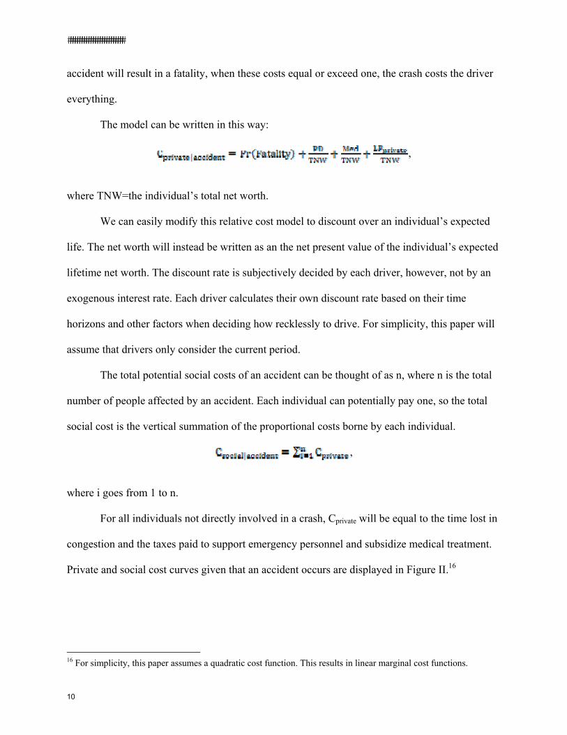
The total potential social costs of an accident can be thought of as n, where n is the total

number of people affected by an accident. Each individual can potentially pay one, so the total

social cost is the vertical summation of the proportional costs borne by each individual.

,

where i goes from 1 to n.

For all individuals not directly involved in a crash, Cprivate will be equal to the time lost in

congestion and the taxes paid to support emergency personnel and subsidize medical treatment.

Private and social cost curves given that an accident occurs are displayed in Figure II.16

16 For simplicity, this paper assumes a quadratic cost function. This results in linear marginal cost functions.

10

�������������������������

An ideal Pigovian tax would increase the marginal private cost so that it equals the

marginal social cost, as in Figure I. However, an ex post Pigovian tax will only increase the costs

if an individual gets into an accident. It will have no effect on the probability of an accident.

Because an individual expects a crash (if it occurs) to cost everything at some level of

recklessness, a Pigovian tax can only increase marginal cost up to that point. We shall designate

the level of recklessness at which the private costs equal one as R*. After R*, private costs will

always equal one and marginal cost will always be zero.17 Driving more recklessly will not

increase an individual’s costs at all. Not only will marginal cost equal zero, but marginal cost

cannot be increased. Since an individual’s cost already equals one, no tax will make the

individual pay any more. After point R*, no tax will have an effect on the level of R.

Since the total cost cannot be increased after R*, it is more accurate to write Cprivate|accident

as a piecewise function.

A Pigovian tax can increase the marginal private cost for all points before R*. The effects

of a Pigovian tax on Cprivate|accident is shown in Figure III. Note that marginal costs must also be

calculated as a proportion of what an individual can pay.18

The costs given that an accident occurs are independent of the probability of a crash.

Likewise, a Pigovian tax will have no effect on the probability of an accident. An individual’s

17 Since the cost function is a piece-wise function, it is not differentiable at R*. 18 For the curves drawn in Figures II and III, approaches ∞ as Cprivate|accident approaches R*. However, since the marginal costs are expressed as a proportion of what an individual can pay, the MCprivate|accident curve approaches 1. MCprivate|accident cannot exceed one.

11

�������������������������

expected cost of an accident is equal to the costs given that he or she is in an accident times the

probability that an accident will occur. So,

,

This is unchanged from the original model, when costs were calculated in absolute, rather than

relative, terms.

Assuming that the probability of a crash increases with R, then Cprivate will continue to

increase, even though Cprivate|accident stops increasing at R*. Cprivate will continue increasing until

both Pr(Accident) and Cprivate|accident equal one, or when an accident occurs with certainty and is

certain to cost the driver everything. We can designate the level of recklessness at which Cprivate

becomes one as R**.

It is important to note that a Pigovian tax still will not affect Cprivate after R* even though

the marginal cost continues increases between R* and R**. Figure IV illustrates these effects.

12

�������������������������

Testing the Model

To determine the possible effects of a Pigovian crash tax, one must determine whether

the equilibrium R is greater than or less than R*. Significant empirical work needs to be done to

determine the level of R as well as the specific shape of an individual driver’s cost curve.

Research such as Cohen and Dehejia (2003) suggests that the equilibrium R is to the left

of R*. Compulsory insurance and no-fault liability laws shift an individual driver’s cost curve to

the right. Rather than increase the marginal cost, as a Pigovian tax would, these laws decrease

the costs a driver faces.

For all values of R greater than R*, marginal costs are equal to zero and no tax can alter a

driver’s behavior. Cohen and Dehejia find that implementing compulsory insurance and no-fault

liability laws increase the fatality rate. Since these policies affect drivers’ behavior, they suggest

that R is initially to the left of R*.19

It is certainly true that the expected private costs of an accident do not exceed one in all

situations. But it is also likely that there are many situations where the expected private costs do

exceed one. To figure out when a crash tax will have an effect, it is necessary to discover what

factors influence a driver’s decision of R and how the level of R affects the cost and probability

of a crash.

Reports such as the National Highway Traffic Safety Administration’s “National Motor

Vehicle Crash Causation Survey” (2008) shed significant light on which actions are associated

19 Paradoxically, when R is greater than R*, policies that reduce a driver’s marginal cost can actually lower the accident rate under the right circumstances. See Figure V for an analysis of how this would occur.

13

�������������������������

with a higher probability of an accident.20 I am aware of no studies, however, on reports that

calculate the costs of an accident under given circumstances.

How much is an accident expected to cost for a driver with a given lifetime expected net

worth, driving a given type of car, going a given speed, on a given road at a given time of day,

and allocating a given amount of his or her attention to driving? This is not an easy question to

answer by any means.

The U.S. Department of Transportation has set the value of a statistical life (VSL) at $6.0

million when preparing economics analyses.21 Assuming that $6.0 million is the correct

monetary value of an individual’s life,22 then R* will occur where the total private cost curve

reaches $6.0 million. A crash tax will not fully internalize social costs if the total social cost of

the accident exceeds $6.0 million.

20 The survey examines 5,471 accidents and determines their cause. The report calculates what the chances are of a certain activity being the cause of a crash, given that a crash occurs. It does not predict the probability that a driver who acts in a certain way will be in a crash. These data are much harder to come by. As Levitt and Porter (2001) write about the probability of alcohol consumption causing a crash:

Without knowing the fraction of drivers on the road who have been drinking, however, one cannot possibly draw conclusions about the relative fatal crash risk of drinking versus sober drivers, the externality associated with drinking and driving, or the appropriate policy response. For instance, if 30 percent of the drivers had been drinking, over half of all two-vehicle crashes would be expected to involve at least one drinking driver, even if drinking drivers were no more dangerous than sober drivers. (1199)

Likewise, it is impossible to know how much reckless driving actually increases the chances of being in an accident and the likely severity of that accident unless one also knows how many drivers drive recklessly. Not only that, but one would have to know precisely how recklessly each individual was driving.

21 The Department of Transportation adopted a recommended VSL at $2.5 million in 1993. This value has been updated periodically, with the latest previous adjustment being in 2002, when the value was set at $3.0 million. Recently, the value has been increased to $5.8 million. See Szabat and Knapp (2009). 22 The DOT is certain to point out that $5.8 million is just an estimate, not “a threshold dividing justifiable from unjustifiable actions” (Duvall and Gribbin, 2008). However, for the purposes of this paper, we can assume that $5.8 million is a uniform VSL for all individuals in all situations. It is also important to note that DOT derives the VSL from individuals’ willingness to pay for reductions in risk. It does not and cannot measure an individual’s actual valuation of his or her life.

14

�������������������������

How likely is it that a crash will cost society more than $6.0 million? Since the VSL is

$6.0 million, any fatal crash will by definition cost at least that much. The National Highway

Traffic Safety Administration reports that 0.8% of crashes result in a fatality.23

Another 10.5% of crashes resulted in incapacitating injuries.24 We can assume that

incapacitating injuries cost an individual nearly $6.0 million. It is easy to believe that property

damage and external costs put the total social costs of these accidents above the threshold level.

Thus, almost eleven percent of traffic crashes will be unaffected by a crash tax.

But even more crashes may be impervious to Pigovian taxation. The percentage of

crashes that cost more than $6.0 million would surely be higher when congestion and other social

costs are factored in. Even though estimates of the aggregate social cost exist, far more work

needs to be done to calculate the social cost generated per accident.

Blincoe et al. (2002) report that 16,352,041 accidents occurred in 2000. These cost the

people involved a total of $230.6 billion. This amounts to an average cost of only $14,100 per

accident, far below the $6.0 million estimated VSL.25 Factoring in social costs is unlikely to push

the average cost above $6.0 million.

Even though the average cost of accidents falls below the R* value, some driving

behaviors lead to higher crash costs than others. Knowing the average cost of an accident is less

useful than knowing how a marginal increase in recklessness affects the expected costs of an

accident. Likewise, it would be useful to learn the expected costs of an accident under certain

specific conditions.

23 National Highway Traffic Safety Administration (2008). 24 Ibid. 25 The VSL in 2000 was estimated to be less than $3.0 million, however. The $6.0 million VSL came into effect in 2009. Thus the VSL in 2000 was less than half of its 2009 value.

15

�������������������������

Significant research is needed to determine what actions make up the aggregated

variable R. In addition, more work needs to be done to discover how the R value affects the

expected costs of an accident.

Results and Conclusion

More research is required to figure out how the components of the variable R are related

to one another. How does a driver make decisions in risky situation with limited time to consider

options? How do those decisions influence the chance of a crash and the expected costs of an

accident? When does a driver reach the threshold value R*?

These questions will all have to be answered before a policy analyst can make

recommendations about the potential for a crash tax. In spite of these unknowns, we can already

make several conclusions about the model.

For one thing, it is clear that automobile crashes create significant externalities. An

optimal policy will internalize these social costs. Pigovian taxes are already used to combat a

number of traffic-related externalities.

In a standard external cost model, a Pigovian crash tax will be able to internalize all

externalities caused by traffic accidents. Modifying the model suggests, however, that the

potential of a Pigovian tax will be limited.

The model created in this paper differs from the standard external cost model in that it

calculates costs as a fraction of an individual’s ability to pay. The standard model calculates

costs as an absolute value, ignoring how much an individual can pay. Under the modified model,

there exists some threshold value at which an individual pays everything. At this point, total

costs are constant and marginal costs equal zero.

16

�������������������������

Individuals will only respond to incentives until they reach their maximum ability to pay.

Once an individual pays everything, no tax can make that individual pay more. Thus, when

individuals are paying everything they can, Pigovian taxes will not solve externality problems.

An example may be helpful. It is not unreasonable to assume that a crash could cost

society ten million dollars. We can also assume that a driver expects their total lifetime net worth

to equal only eight million dollars. Standard theory states that an appropriate tax can force an

individual to act as if he would pay all ten million dollars. But in this example, the driver will

never have ten million dollars. He will not internalize the remaining two million dollars that the

crash causes. Even after the tax, an externality remains.

If a driver does not value the future highly, then a tax will be even less effective.

Regardless of an individual’s expected lifetime net worth, few people have ten million dollars to

their name at any given time. A driver with a short time horizon may behave as though they only

have a few million dollars at risk. This will lead to a greater level of costs that are not

internalized.

Harvard’s Gregory Mankiw has created an informal group that he calls the Pigou Club.

This group is made up of individuals who believe that Pigovian taxes are the best way to

eliminate externalities. Mankiw (2006) lists four possible reasons why individuals might be

opposed to Pigovian taxes. But Mankiw never considers the possibility that, in some instances,

Pigovian taxes may simply have no effect on an individual’s behavior.

This paper identifies one such situation. If an individual expects a crash to cost

everything if it occurs, then he or she may seek to minimize the chances of a crash. If the

benefits of reckless driving are large, then an individual may still engage in the activity. If this

17

�������������������������

happens, the driver will behave the same way regardless of whether or not an ex post Pigovian

crash tax is in place.

At the very least, this model suggests that a Pigovian tax is not appropriate in all

instances where externalities are present. In the case of traffic accidents, the crashes that cost

society the most are precisely those that will not be affected by a tax. Other methods must be

used to bring the level of recklessness on the road to the socially optimal level.26

Calculating costs as a fraction of what an individual can pay substantially changes the

standard external cost model. A Pigovian tax will not correct externalities when individuals face

costs that exceed their total ability to pay. It remains to be seen how common this phenomenon is

in real crash situations.

26 More precisely, other methods must be used to bring the level of recklessness to less than R*. For values to the left of R*, a Pigovian tax will be effective.

18

�������������������������

References

Blincoe, Lawrence J., Angela G. Seay, Eduard Zaloshnja, Ted R. Miller, Eduardo O. Romano, Stephen Luchter, and Rebecca S. Spicer, The Economic Impact of Motor Vehicle Crashes 2000, DOT HS 809 446, Washington, DC: U.S. Department of Transportation, National Highway Traffic Safety Administration (2002). http://www.cmfclearinghouse.org/collateral/Economic_Impact_of_Motor_Vehicle_Crashes.PDF.

Cohen, Alma, and Rajeev Dehejia, “The Effect of Automobile Insurance and Accident Liability Laws on Traffic Fatalities,” NBER Working Paper No. w9602, National Bureau of Economic Research, Cambridge, MA, 2003. http://www.nber.org/papers/w9602.pdf.

Davis, Stacy C., and Susan W. Diegel, “Fuel Economy by Vehicle Speed,” in Transportation Energy Data Book: Edition 22 (Oak Ridge, TN: Center for Transportation Analysis, Engineering Science and Technology Division, 2002), 7-24-7-28. http://www-cta.ornl.gov/cta/Publications/Reports/ORNL-6967.pdf.

Duvall, Tyler D., and J.D. Gribbin, “Treatment of the Economic Value of a Statistical Life in Departmental Analyses,” memorandum for the Office of the Secretary of Transportation (2008). http://ostpxweb.dot.gov/policy/reports/080205.htm.

Edlin, Aaron S., and Pinar Karaca-Mandic, “The Accident Externality from Driving,” Journal of Political Economy 114 (2006), 931-955. http://www.jstor.org/stable/10.1086/508030.

Gayer, Ted, “The Fatality Risks of Sport-Utility Vehicles, Vans, and Pickups Relative to Cars,” Journal of Risk and Uncertainty 28 (2004), 103-133.

Leape, Jonathan, “The London Congestion Charge,” Journal of Economic Perspectives 20 (2006), 157-176. http://www.jstor.org/stable/30033688.

Levitt, Steven D., and Jack Porter, “How Dangerous Are Drinking Drivers?” Journal of Political Economy 109 (2001), 1198-1237. http://www.jstor.org/stable/10.1086/323281.

Mankiw, N. Gregory, “Smart Taxes: An Open Invitation to Join the Pigou Club” (paper based on a presentation at the Eastern Economic Association, March 8, 2008). http://www.economics.harvard.edu/files/faculty/40_Smart%20Taxes.pdf.

Mankiw, N. Gregory, “Alternatives to the Pigou Club”, Greg Mankiw’s Blog, October 26, 2006, http://gregmankiw.blogspot.com/2006/10/alternatives-to-pigou-club.html.

Miller, Ted R., “Societal Costs of Transportation Crashes,” in The Full Costs and Benefits of Transportation: Contributions to Theory, Methods, and Measurement, ed. David L. Greene, Donald W. Jones, and Mark A. Delucchi (Berlin: Springer-Veriag, 1997), 281-308.

Miller, T.R., B. Lawrence, A. Jensen, G. Waehrer, R. Spicer, D. Lestina, M. Cohen, Estimating the Cost to Society of Consumer Product Injuries: The Revised Injury Cost Model, Bethesda, MD: U.S. Consumer Product Safety Commission (1998).

Parry, Ian W. H., and Kenneth A. Small, “Does Britain or the United States Have the Right Gasoline Tax?” American Economic Review 95 (2005), 1276-1289. http://www.jstor.org/stable/4132715.

Parry, Ian W. H., Margaret Walls, and Winston Harrington, “Automobile Externalities and Policies,” Journal of Economic Literature 45 (2007), 373-399. http://www.jstor.org/stable/27646797.

19

�������������������������

Pigou, Alfred C., The Economics of Welfare, 2009 ed. (London: Macmillian, 1920; New Brunswick: Transaction Publishers, 2009), 172-203.

Rice, D.P., E.J. MacKenzie, A.S. Jones, S.R. Kaufman, G.V. deLissovoy, W. Max, E. McLoughlin, T.R. Miller, L.S. Robertson, D.S. Salkever, and G.S. Smith, Cost of Injury in the United States: A Report to Congress, Washington, DC: U.S. Department of Transportation, National Highway Traffic Safety Administration (1989).

Santos, Georgina, “London Congestion Charging,” Brookings-Wharton Papers on Urban Affairs (2008), 177-234. https://muse.jhu.edu/journals/brookings-wharton_papers_on_urban_affairs/v2008/2008.santos.pdf.

Sitkin, Sim B., and Amy L. Pablo, “Reconceptualizing the Determinants of Risk Behavior,” Academy of Management Review 17 (1992), 9-38. http://www.jstor.org/stable/258646.

Szabat, Joel, and Lindy Knapp, “Treatment of the Economic Value of a Statistical Life in Departmental Analyses – 2009 Annual Revision,” memorandum for the Office of the Secretary of Transportation (2009). http://ostpxweb.dot.gov/policy/reports/VSL%20Guidance%20031809%20a.pdf.

U.S. Department of Transportation, National Highway Traffic Safety Administration, National Motor Vehicle Crash Causation Survey, DOT HS 811 059 (2008). http://www-nrd.nhtsa.dot.gov/Pubs/811059.PDF.

White, Michelle J., “The ‘Arms Race’ on American Roads: The Effect of Sport Utility Vehicles and Pickup Trucks on Traffic Safety,” Journal of Law and Economics 47 (2004), 333-355. http://www.jstor.org/stable/10.1086/422979.

20

�������������������������

Figure I

Figure I presents the standard external cost model. An optimal marginal tax can shift the marginal private cost curve so that the new Rprivate equals Rsocial at the optimal level of R.

21

�������������������������

Figure II

In this graph we assume quadratic total cost curves. The private cost curve (given that an accident occurs) will increase quadratically until R*. The social cost curve (given that an accident occurs) will increase quadratically until every driver is paying one. This occurs at n*1.

22

�������������������������

Figure III

The marginal cost curves (given that an accident occurs) in this graph are derived from the total cost curves displayed in Figure II. The marginal private cost curve is shown by a dotted line. The optimal marginal tax will shift the marginal private cost curve to the left. However, when the new marginal private cost curve reaches C=1, it falls to 0. So a marginal tax will shift R* to the left. Since marginal costs are 0 after R*, the marginal benefit curve intersects the marginal private cost curve at MCprivate=0.

23

�������������������������

Figure IVa

24

�������������������������

Figure

IVc

Figure IVa displays the total private cost. Note that the private cost increases quadratically from 0 to R*. IVa increases linearly from R* to R** as the cost becomes a function solely of the probability. After R**, IVa is flat. Figure IVb displays the marginal private costs. As in Figure III, marginal costs are displayed as a dotted line. Figure IVc combines Figures IVa and IVb, along with a marginal social cost curve and a marginal benefit curve. Figure IVc also displays the optimal marginal tax. As in Figure III, a marginal tax shifts R* to the left and a marginal tax will have no effect after R*. In this case, however, the marginal benefit curve will intersect the marginal private cost curve when MCprivate=1*p.

25

�������������������������

Figure V

An activity that decreases an individual’s marginal cost may have the paradoxical effect of reducing Req, as shown in Figure V. This result depends on the specific shape of the marginal benefits curve and the magnitude of the marginal cost reduction.

26