P. 1 DSP-II Digital Signal Processing FIR Filter Design Marc Moonen Dept. E.E./ESAT, K.U.Leuven

p. 1DSP-II

Digital Signal Processing

FIR Filter Design

Marc Moonen

Dept. E.E./ESAT, K.U.Leuven

FIR Filter Design

• Review of discrete-time systems LTI systems, impulse response, transfer function, ...

• FIR filters

Direct form, Lattice, Linear-phase filters

• FIR design by optimization

Weighted least-squares design

Minimax design

• FIR design using `windows’• Equiripple design• Software (Matlab,…)

Review of discrete-time systems 1/10

Linear time-invariant (LTI) systems

• Linear :

input u1[k] -> output y1[k]

input u2[k] -> output y2[k]

hence input a.u1[k]+b.u2[k]-> a.y1[k]+b.y2[k]

• Time-invariant (shift-invariant)

input u[k] -> output y[k]

hence input u[k-T] -> output y[k-T]

u[k] y[k]


Linear time-invariant (LTI) systems

• Causal systems:

for all input u[k]=0, k<0 -> output y[k]=0, k<0

• Impulse response :

input 1,0,0,0,... -> output h[0],h[1],h[2],h[3],...

input u[0],u[1],u[2],u[3] -> output y[0],y[1],y[2],y[3],...

= `convolution’

u[k] y[k]

][*][][].[][ khkuikhiukyi


• Impulse response/convolution:

][*][][].[][ khkuikhiukyi

]3[

]2[

]1[

]0[

.

]2[000

]1[]2[00

]0[]1[]2[0

0]0[]1[]2[

00]0[]1[

000]0[

]5[

]4[

]3[

]2[

]1[

]0[

u

u

u

u

h

hh

hhh

hhh

hh

h

y

y

y

y

y

y

u[0],u[1],u[2],u[3],0,0…. y[0],y[1],...

h[0],h[1],h[2],0,0,...

`Toeplitz’ matrix


• Z-Transform:

i

izihzH ].[)(

]3[

]2[

]1[

]0[

.

]2[000

]1[]2[00

]0[]1[]2[0

0]0[]1[]2[

00]0[]1[

000]0[

.1

]5[

]4[

]3[

]2[

]1[

]0[

.1

3211).()(

5432154321

u

u

u

u

h

hh

hhh

hhh

hh

h

zzzzz

y

y

y

y

y

y

zzzzz

zzzzHzY

i

iziyzY ].[)( i

iziuzU ].[)(

)().()( zUzHzY


Z-Transform :• input-output relation • `shorthand’ notation

(for convolution operation/Toeplitz-vector product)

• stability

bounded input u[k] -> bounded output y[k]

--iff

--iff poles of H(z) inside the unit circle

(for causal,rational systems)

)().()( zUzHzY

k

kh ][


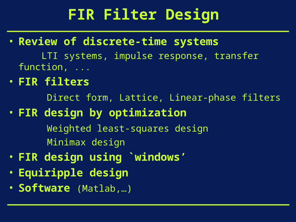
Frequency response :• given a system with impulse response h[k] • given an input signal = complex sinusoid

• output signal :

is `frequency response’

is H(z) evaluated on the unit circle

keku kj ,][

jezi

ijkj

i

ikj

i

zHkxeiheeihikxihky

)(].[].[].[][].[][ )(

)( jeH


Frequency response :• for a real impulse response h[k]

Magnitude response is even function

Phase response is odd function• example :

)( jeH

)( jeH

-4 -2 0 2 40

0.5

1

-4 -2 0 2 4-5

0

5

Nyquist frequency

,...1,1,1,1,1..., kje


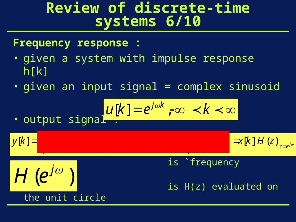
`Popular’ frequency responses for filter design :

low-pass (LP) high-pass (HP) band-pass (BP)

band-stop multi-band


Rational transfer functions (ÌIR filters’):•

• N poles (zeros of A(z)) , N zeros (zeros of B(z))• corresponds to difference equation

NN

NN

zaza

zbzbb

zA

zBzH

...1

...

)(

)()(

11

110

][....]1[.][.][....]1[.][ 101 NkubkubkubNkyakyaky NN

][....]1[.][....]1[.][.][ 110 NkyakyaNkubkubkubky NN


`FIR filters’ (finite impulse response):•

• `Moving average filters’ (MA)• N poles at the origin z=0 (hence guaranteed stability) • N zeros (zeros of B(z)), àll zero’ filters• corresponds to difference equation

• impulse response

NN zbzbbzBzH ...)()( 1

10

][....]1[.][.][ 10 Nkubkubkubky N

,...0]1[,][,...,]1[,]0[ 10 NhbNhbhbh N

Review of discrete-time systems

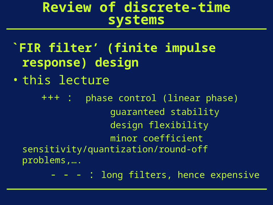
`FIR filter’ (finite impulse response) design

• this lecture +++ : phase control (linear phase)

guaranteed stability

design flexibility

minor coefficient sensitivity/quantization/round-off problems,….

- - - : long filters, hence expensive

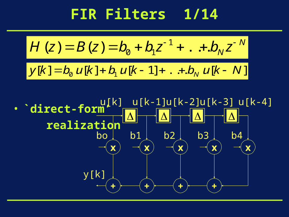
FIR Filters 1/14

• `direct-form’

realization

u[k]

u[k-4]u[k-3]u[k-2]u[k-1]

xbo

+

xb4

xb3

+

xb2

+

xb1

+y[k]

NN zbzbbzBzH ...)()( 1

10

][....]1[.][.][ 10 Nkubkubkubky N

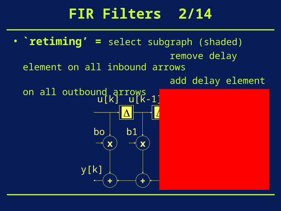
FIR Filters 2/14

• `retiming’ = select subgraph (shaded)

remove delay element on all inbound arrows

add delay element on all outbound arrows

u[k]

u[k-4]u[k-3]u[k-2]u[k-1]

xbo

+

xb4

xb3

+

xb2

+

xb1

+y[k]

FIR Filters 3/14

• `retiming’ : results in...

u[k]

u[k-1]

xbo

+

xb1

+y[k]

u[k-3]u[k-2]

xb4

xb3

+

xb2

+

FIR Filters 4/14

• `retiming’ : repeated application results in...

`Transposed direct-form’ realization

u[k]

xbo

+y[k]

xb1

+

xb2

+

xb3

+

xb4

FIR Filters 5/14

• `Lattice form’ : derived from combined realization with

reversed coefficient vector results in

- same magnitude response

- different phase response

][....]1[.][.][ 10 Nkubkubkubky N

][....]1[.][.][ 01 Nkubkubkubky NN

FIR Filters 6/14

• `Lattice form’ : derivation (I)

u[k] u[k-1]

u[k-2]

xb1

+

xb2

+

x

+

x

+

b3

u[k-3]

xb3

+

b2 x

+

xbo

+

y[k]

b4x

+y[k]

u[k-4]

xb4

b1 x bo

FIR Filters 7/14

• `Lattice form’ : derivation (II), this is equivalent to...

(=simple proof)

u[k] u[k-1]

u[k-2]

xb’1

+

xb’2

+

x

+

x

+

b’3

u[k-3]

xb’3

+

b’2 x

+

xb’o

+

y[k] 0x

+y[k]

u[k-4]

x0

b’1 x b’o+

+

x

xko

...,...,...,,, '3

'2

'10

'0

0

40 bbbbb

b

bk

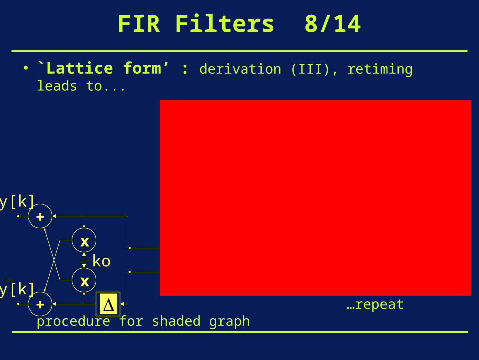
FIR Filters 8/14

• `Lattice form’ : derivation (III), retiming leads to...

…repeat procedure for shaded graph

u[k] u[k-3]

u[k-2]

xb’o

+

xb’1

+

x

+

x

+

b’3

u[k-2]

xb’2

+

b’2 x

+

b’3

y[k]

y[k]

xb’1 x b’o

+

+

x

xko

FIR Filters 9/14

• `Lattice form’ : derivation (IV), end result is...

u[k]

y[k]

y[k]

+

+

x

xko

+

+

x

xk1

+

+

x

xk2

+

+

x

xk3

xk4

FIR Filters 10/14

`Lattice form’ : • ki’s are `reflection coefficients’

• procedure for computing ki’s from bi’s corresponds to `Schur-Cohn’ stability test (control theory):

all zeros of B(z) are stable (i.e. lie inside unit circle)

iff all reflection coefficients statisfy |ki|<1 (i=1,…,N-1)

(ps: procedure breaks down if |ki|=1 is encountered)

FIR Filters 11/14

Linear-phase FIR filters• Non-causal zero-phase filters :

example: symmetric impulse response

h[-L],….h[-1],h[0],h[1],...,h[L]

h[k]=h[-k], k=1..L

frequency response is

- real-valued (=zero-phase) transfer function

- causal implementation by introducing (group) delay

L

k

L

Lk

kjj kkaekheH0

. ).cos(].[...].[)(

kL

FIR Filters 12/14

Linear-phase FIR filters• Causal linear-phase filters :

example: symmetric impulse response & N even

h[0],h[1],….,h[N]

N=2L (even)

h[k]=h[N-k], k=0..L

frequency response is

- causal implementation of zero-phase filter, by

introducing (group) delay

L

k

LjN

k

kjj kkaeekheH00

. ).cos(].[....].[)(

kN

Lj

ez

L ezj

0

FIR Filters 13/14

Linear-phase FIR filters

Type-1 Type-2 Type-2 Type-4

N=2L=even N=2L+1=odd N=2L=even N=2L+1=odd

symmetric anti-symmetric symmetric anti-symmetric

h[k]=h[N-k] h[k]=-h[N-k] h[k]=h[N-k] h[k]=-h[N-k]

zero at zero at zero at

LP/HP/BP LP/BP HP

L

k

Nj kkae0

2/ ).cos(].[.

L

k

Nj kkae0

2/ ).cos(].[).2

cos(

L

k

Nj kkaej0

2/ ).cos(].[).2

sin(.

1

0

2/ ).cos(].[).sin(L

k

Nj kkae

,0 0

FIR Filters 14/14

Linear-phase FIR filters• efficient direct-form realization.

example:

bo

y[k]

u[k]

+

+ ++ +

++

x xb4

xb3

xb2

xb1

++

Filter Design by Optimization

(I) Weighted Least Squares Design :• select one of the basic forms that yield linear phase

e.g. Type-1

• specify desired frequency response (LP,HP,BP,…)

e.g.: LP

• optimization criterion is

where is a weighting function

)(.).cos(].[.)( 2/

0

2/ AekkaeeH NjL

k

Njj

)(.)( 2/ d

Njd AeH

dAAWdHeHWaaF ddj

L

22

0 )()()()()()(),...,(

0)( W

edge) stopband ( ,0)(

edge) passband ( ,1)(

S

P

Sd

Pd

A

A


• …this is equivalent to

i.e. convex `Quadratic Optimization’ problem• this is often supplemented with additional constraints...

constant

)cos(...)cos(1)(

)().().(

)().().(

...

.2..),...,(

0

0

10

0

Lc

dcAWb

dccWQ

aaax

bxxQxaaF

T

d

T

LT

TTL


Example: Low-pass (LP) design

optimization criterion is

an additional constraint may be imposed to control the pass-band ripple …

… as well as the stop-band ripple

bxxQxdAdAaaF TTL

S

P

.2..)(.1)(),...,( 2

0

2

0

edge) (stopband ,0)(

edge) (passband ,1)(

Sd

Pd

A

A

ripple) passband is ( ,1)( PP PA

ripple) stopband is ( ,)( SS SA

PS: Filter Specification

0 0.5 1 1.5 2 2.5 30

0.2

0.4

0.6

0.8

1

1.2

Passband Ripple

Stopband Ripple

Passband Cutoff -> <- Stopband Cutoff

S

P SP1

Filter Design using `Windows’

Example : Low-pass filter design• ideal low-pass filter is

• hence ideal time-domain impulse response is

• truncate hd[k] to N+1 samples :

• add (group) delay to turn into causal filter

0

1)(

C

CdH

k

kdeeHkh

c

cjdd

kj

)sin(....).(

2

1][

otherwise 0

2/2/ ][][

NkNkhkh d


Example : Low-pass filter design (continued)• it can be shown that this corresponds to the solution of weighted least-

squares optimization with the given Hd, and weighting function for all freqs.

• truncation corresponds to applying a `rectangular window’ :

• +++: simple procedure (also for HP,BP,…)• - - - : truncation in the time-domain results in `Gibbs effect’ in the

frequency domain, i.e. large ripple in pass-band and stop-band, which cannot be reduced by increasing the filter order N.

][].[][ kwkhkh d

otherwise 0

1][

2/2/ NkNkw

1)( W


Remedy : apply windows other than rectangular window:• time-domain multiplication with a window function w[k] corresponds to

frequency domain convolution with W(z) :

• candidate windows : Han, Hamming, Blackman, Kaiser,…. (see textbooks, see DSP-I)

• window choice/design = trade-off between side-lobe levels (define peak pass-/stop-band ripple) and width main-lobe (defines transition bandwidth)

][].[][ kwkhkh d

)(*)()( zWzHzH d

Design Procedure• To fully design and implement a filter five steps are required:

(1) Filter specification.

(2) Coefficient calculation.

(3) Structure selection.

(4) Simulation (optional).

(5) Implementation.

Filter Specification - Step 1

(a)

1

f(norm)fc : cut-off frequency

pass-band stop-band

pass-band stop-bandtransition band

1

s

pass-bandripple

stop-bandripple

fpb : pass-band frequency

fsb : stop-band frequency

f(norm)

(b)

p1

s

p0

-3

p1

fs/2

fc : cut-off frequency

fs/2

|H(f)|(dB)

|H(f)|(linear)

|H(f)|

Coefficient Calculation - Step 2• There are several different methods available, the most popular are:

– Window method.– Frequency sampling.– Parks-McClellan.

• We will just consider the window method.

Window Method

• First stage of this method is to calculate the coefficients of the ideal filter.• This is calculated as follows:

0nfor

0nfor

2

sin2

12

1

2

1

c

c

cc

nj

njd

fn

nf

de

deHnh

c

c

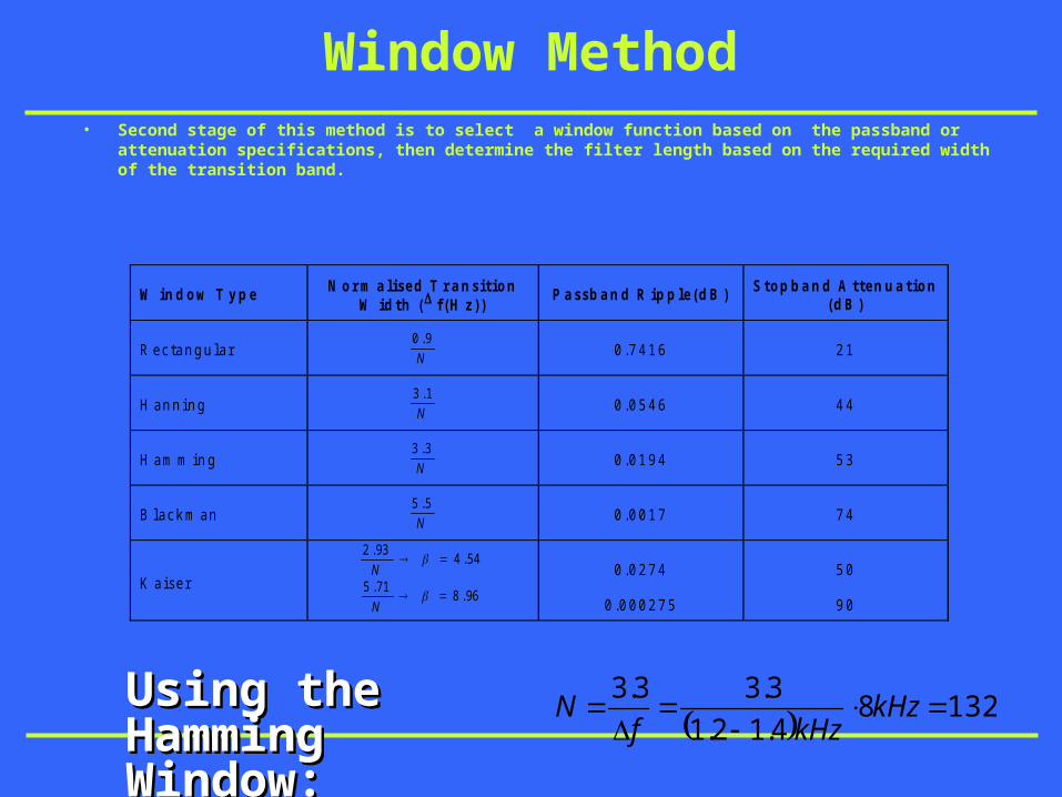
Window Method• Second stage of this method is to select a window function based on the passband or attenuation

specifications, then determine the filter length based on the required width of the transition band.

W i n d o w T y p e N o r m a l i s e d T r a n s i t i o nW i d t h ( f ( H z ) )

P a s s b a n d R i p p l e ( d B ) S t o p b a n d A t t e n u a t i o n( d B )

R e c t a n g u l a rN

9.00 . 7 4 1 6 2 1

H a n n i n gN

1.30 . 0 5 4 6 4 4

H a m m i n gN

3.30 . 0 1 9 4 5 3

B l a c k m a nN

5.50 . 0 0 1 7 7 4

K a i s e r

54.493.2

N

96.871.5

N

0 . 0 2 7 4

0 . 0 0 0 2 7 5

5 0

9 0

13284.12.1

3.33.3

kHz

kHzfNUsing the Hamming Using the Hamming

Window:Window:

Window Method

• The third stage is to calculate the set of truncated or windowed impulse response coefficients, h[n]:

nWnhnh d even Nfor

odd Nfor

22

2

1

2

1

Nn

N

Nn

N

133

2cos46.054.0

2

cos46.054.0

n

N

nnW

forfor

Where:Where:6666 nforfor

Window Method

• Matlab code for calculating coefficients:close all;clear all;

fc = 8000/44100; % cut-off frequencyN = 133; % number of tapsn = -((N-1)/2):((N-1)/2);n = n+(n==0)*eps; % avoiding division by zero

[h] = sin(n*2*pi*fc)./(n*pi); % generate sequence of ideal coefficients[w] = 0.54 + 0.46*cos(2*pi*n/N); % generate window functiond = h.*w; % window the ideal coefficients

[g,f] = freqz(d,1,512,44100); % transform into frequency domain for plotting

figure(1)plot(f,20*log10(abs(g))); % plot transfer functionaxis([0 2*10^4 -70 10]);

figure(2);stem(d); % plot coefficient valuesxlabel('Coefficient number');ylabel ('Value');title('Truncated Impulse Response');

figure(3)freqz(d,1,512,44100); % use freqz to plot magnitude and phase responseaxis([0 2*10^4 -70 10]);

Window Method

0 0.5 1 1.5 2

x 104

-6000

-4000

-2000

0

Frequency (Hz)

Pha

se (

degr

ees)

0 0.2 0.4 0.6 0.8 1 1.2 1.4 1.6 1.8 2

x 104

-60

-40

-20

0

Frequency (Hz)

Mag

nitu

de (

dB)

0 20 40 60 80 100 120 140-0.1

0

0.1

0.2

0.3

0.4

Coefficient number

Val

ue

Truncated Impulse Response

Equiripple Design

• Starting point is minimax criterion, e.g.

• Based on theory of Chebyshev approximation and the àlternation theorem’, which (roughly) states that the optimal ai’s are such that the `max’ (maximum weighted approximation error) is obtained at L+2 extremal frequencies…

…that hence will exhibit the same maximum ripple (èquiripple’)• Iterative procedure for computing extremal frequencies, etc. (Remez

exchange algorithm, Parks-McClellan algorithm) • Very flexible, etc., available in many software packages• Details omitted here (see textbooks)

)(maxmin)()().(maxmin),...,( 0,...,0,...,0 00 EAAWaaF

LL aadaaL

2,..,1for )()(max0 LiEE i

Software

• FIR Filter design abundantly available in commercial software

• Matlab:

b=fir1(n,Wn,type,window), windowed linear-phase FIR design, n is filter order, Wn defines band-edges, type is `high’,`stop’,…

b=fir2(n,f,m,window), windowed FIR design based on inverse fourier transform with frequency points f and corresponding magnitude response m

b=remez(n,f,m), equiripple linear-phase FIR design with Parks-McClellan (Remez exchange) algorithm

Documents

P. 1 DSP-II Digital Signal Processing FIR Filter Design Marc Moonen Dept. E.E./ESAT, K.U.Leuven