JOURNAL OF HYDROLOGY (N.Z.) Vol. 9, No. 2, 197U

OVERLAND FLOW ON RANGELAND WATERSHEDS*

D. A. Woolhiser, C. L. Hanson and A. R. Kuhlmanf

ABSTRACT

The kinematic cascade was used as a mathematical model to describeoverland and open-channel flow for small (0.81-hectare) rangeland watersheds. The friction relationship for overland flow was assumed to be of theDarcy-Wcisbach form, with initially laminar flow becoming turbulent ata transitional Reynolds number of 300. For laminar flow, the Darcy-Wcisbach friction factor / can be expressed as

where A: is a parameter and NR is the Reynolds number.Optimum values of the parameter k were obtained by a univariate

optimization procedure for four heavily grazed watersheds and four lightlygrazed watersheds for a single storm. Although these watersheds showedsubstantial differences in vegetal composition and cover in weight of vegetation per unit area, the roughness parameters were not significantly different.The average of the eight optimized parameters was used in the kinematic-cascade model to predict hydrographs for four moderately grazed watersheds with very good results.

The kinematic-cascade model appears to be satisfactory for describingoverland flow on small rangeland watersheds. The roughness parameter k inthe laminar friction relationship is approximately "7,000 for native short-grass prairie rangelands in western South Dakota, U.S.A.

INTRODUCTION

The shallow-water equations, or an approximation to themcalled the kinematic-wave equation, may be used as physically-based, deterministic models of overland and open-channel flow.A functional relationship between the friction slope, Sf, the meanvelocity, w, the hydraulic radius, R, and some measure of thesurface roughness characteristics is an essential element in theshallow-water equations and serves as the defining relationship

♦ Contribution from the Northern Plains Branch, Soil and Water Conservation Research Division, Agricultural Research Service, USDA, in cooperation with the Colorado and South Dakota Agricultural ExperimentStations.

t Research Hydraulic Engineer, USDA, Fort Collins, Colorado; AgricultralEngineer, USDA, Rapid City, South Dakota; and Botanist, USDA, Newell,South Dakota.

336 Purchased byUSDA Agric. Research Se]

between u and R in the kinematic-wave approximation. The Manning or Chezy equations are frequently used as the friction relationship for open-channel flow and appear to be satisfactory whenempirical data are available to assist in estimating the roughnesscoefficients.

Experimental evidence indicates that overland flow is initiallylaminar and may become turbulent under certain circumstances(Morgali, 1970; Schaake. 1965; Das and Huggins, 1970; Woo andBrater, 1962; Yu and McNown, 1964).

If the flow is laminar, the parameter k in the friction relationship

f=k/NR (1)

must be estimated, where / is the friction factor in the Darcy-Weisbach formulation and NR is the Reynolds number. Jf the flowis initially laminar but becomes turbulent at higher flow rates, atleast two parameters must be estimated: k as in the laminar case,and either a transitional Reynolds number or a Ch6zy C orManning's n. For a very smooth surface, k can be derived theoretically and has a lower limit of 24. In an analysis of experimentaldata obtained by Izzard (1943), Morgali found that k varied from14 to 35 for smooth asphalt, 20 to 65 for a crushed-slate surfaceand from 5,000 to 14,000 for turf surfaces. No objective techniquehas been developed to estimate the transitional Reynolds number.Morgali (1970) indicates the laminar-to-lurbulenl transition occurring at a Reynolds number of approximately 100 for a turf plane.Yu and McNown (1964) found a transitional Reynolds numberbetween 200 bo 1,000 for flow on a concrete surface. Chow (1959)suggests a range of from 500 to 2,000 for open-channel flow.

It is quite obvious that severe approximations are inherentin the use of the shallow-water equations or the kinematic-waveequations as a model of overland flow over rough planes or onnatural watersheds. If the parameters of the friction relationship

• are estimated by minimizing some measure of the error between=: observed and computed hydrographs, the intrinsic errors introduced[£-" by the original approximations, the geometrical simplification ofjfte'.the natural system, and the estimates of rainfall input and infiltra-!&^- tion, all become lumped into the friction parameters.

!:i>K'-'.:.rft^f Consider a sequence of runoff events from two adjacent,*̂ apparently identical watersheds, and denote the estimated para-j|meters as kit k2, and Cu C2. Because of the simplifications inherent||in the model and natural variability, these parameters will be

[random variables. The question of how variable such parameters[might.be is extremely important if the hydraulic approach is to

s useful for natural watersheds.fe. •&tt 337:Pi-

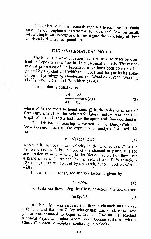
The objective of the research reported herein was to obtainestimates of roughness parameters for overland flow on smallnuner simple watersheds and to investigate the variability of theseempirically determined quantities.

THE MATHEMATICAL MODEL

The kinematic-wave equation has been used to describe overland and open-channel flow in the subsequent analysis. The mathematical properties of the kinematic wave have been considered ingeneral by Lighlhill and Whitham (1955) and for particular application mhydrology by Henderson and Wooding (1964), Wooding(1965), and Kibler and Woolhiser (1970).

The continuity equation is

dA dQ~~+—=g(x,o (2)3/ dx

where A is the cross-sectional area, Q is the volumetric rate ofdischarge. cj(x,() is the volumetric lateral inflow rate per unitlength of channel, and x and / are the space and lime coordinates.

The friction relationship is written in the Darcy-Weisbachform because much of the experimental analysis has used thislorm

«=V[(8*//)S0/t] . (3)where // is the local mean velocity in the x direction, R is thehydraulic radius, Sn is the slope of the channel or plane, g is theacceleration of gravity, and / is the friction factor. For flow overa plane or in wide, rectangular channels, A and R in equations(2) and (3) can be replaced by the depth, h, for a section of unitwidth.

In the laminar range, the friction factor is given by

1=k/NR (4)For turbulent flow, using the Chezy equation, / is found from

/=8*/C2 (5)

In this study it was assumed that flow in channels was alwaysturbulent, and that the Chizy relationship was valid. Flow overplanes was assumed to begin as laminar flow until it reacheda critical Reynolds number, whereupon it became turbulent with aCh6zy C chosen to maintain continuity in velocity.

338

Thus, at transition,

SgS0Il2= CV(V0

where v is the kinematic viscosity, and

kvC V/3At

/ kvC V

(6)

(7)

where /iT is the transition depth. For a given transition Reynoldsnumber, C is a function of the parameter k

C=^[(Sg/k)NR] (8)

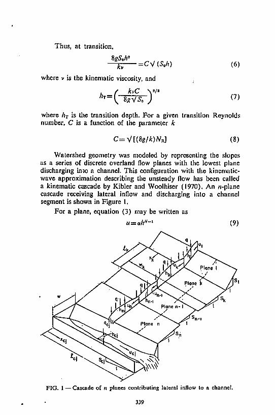
Watershed geometry was modeled by representing the slopesas a series of discrete overland flow planes with the lowest planedischarging into a channel. This configuration with the kinematic-wave approximation describing the unsteady flow has been calleda kinematic cascade by Kibler and Woolhiser (1970). An n-planecascade receiving lateral inflow and discharging into a channelsegment is shown in Figure 1.

For a plane, equation (3) may be written as

u = ahN-1 (9)

FIG. 1 — Cascade of n planes contributing lateral inflow to a channel.

339

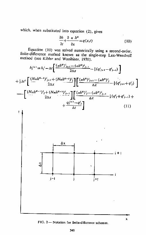
which, when substituted into equation (2), givesdh d a hN

dt dx= q(x,t) (10)

Equation (10) was solved numerically using a second-order,finite-difference method known as the single-step Lax-Wendroffmethod (sec Kibler and Woolhiser, 1970).

/f, -//,-A^— -i(^,+,-^,-,)J

+2^ L- 2A* JL S '-m^+v'i) J[* (Mr/f"-)',-}- (AWl"-')',., 1T(„/,")',._ (a/i")',-..,L 2AJC JL Al ifaW/

Ax

J-I i+i

FIG. 2—Notation for finite-diflercnce schemes.

340

i +

) +

(11)

where the finite-difTerence notation is shown in Figure 2. Thenotation (a/r")'*/+1 indicates that the quantities are evaluated at/A/, (j+l)&x.

The linear stability criterion for this explicit scheme is:

_A/ < 1 (P)AX^/Va/l*"1

An upstream differencing scheme was used at the downstreamboundary of each plane. The discharge from plane n—\ at time/ establishes the upstream boundary condition for plane n at time t.For example, thedischarge per unit width at the upstream boundaryof plane n is

QuM(/)=eL-,(/)-^"^ d3)W (//)

where Qu"(t) is the discharge per unit width at the upper boundaryof plane n\ the subscript L denotes the lower boundary and W( )is the width of the plane.

During calculations each depth /i/+l was checked to see ifit was in the laminar or turbulent range, and the appropriate valuesof a and /V were used in equation (11).

Channels were assumed to be triangular or trapezoidal incross-section. A finite-difTerence equation analogous to equation(11) was used for channel computations. Discharges from contributing channels were added at channel junctions.

THE EXPERIMENTAL WATERSHEDS

Twelve small watersheds of approximately 2 acres (0.81hectares) each were chosen for this analysis. These watersheds arclocated on ths Range Field Station (Figure 3), Cottonwood. SouthDakota, U.S.A. A substation of the South Dakota AgriculturalExperiment Station, it is at an elevation of 2,414 feet (736 m)and is located at latitude 43° 58' and longitude 101° 52'.

The mean annual precipitation at the Field Station headquarters for the period 1910 through 1967 was 15.22 inches(387 mm) and has ranged from 7.13 inches (181mm) in 1936to 27.62 inches (703 mm) in 1915 (Spuhler et «/., 1968). Duringthe growing season, thunderstorms are associated with most of theprecipitation, and therefore there is a wide range in amounts andintensities of rain. June is the month of highest precipitation withan average of 2.99 inches (76 mm). The driest is December whenthe average precipitation is 0.35 inch (9 mm).

341

M«.ES0CITY

o SHERIDAN

N

oCHEYENNE

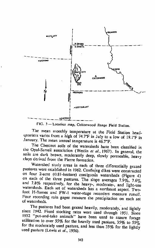
FIG. 3—Location map, Cottonwood Range Field Station.

The mean monthly temperature at the Field Station headquarters varies from a high of 74.7°F in July to a low of I9.PF inJanuary. The mean annual temperature is 46.7T.

The Chestnut soils of the watersheds have been classified inthe Opal-Samsil association (Westin et aL, 1967). In general, thesoils are dark brown, moderately deep, slowly permeable, heavyclays derived from the Pierre formation.

Watershed study areas in each of three differentially grazedpastures were established in 1962. Confining dikes were constructedon four 2-acre (0.81-hectare) contiguous watersheds (Figure 4)on each of the three pastures. The slope averages 79% 76<7and 78% respectively, for the heavy-, moderate-, and light-usewatersheds. Each set of watersheds has a northeast aspect. Two-foot H-flumes and FW-1 water-stage recorders measure runoffI'our recording rain gages measure the precipitation on each setof watersheds.

The pastures had been grazed heavily, moderately, and lightlysince 1942. Fixed slocking rates were used through 1951. Since1952 "put-and-take animals" have been used to assure forageutilization to over 55% for the heavily used pasture, 35% to 55%for the moderately used pasture, and less than 35% for the lightlyused pasture (Lewis et aL, 1956).

342

JLLT-tfiE

:•• Sim AM 0* W4INACX.

-<1 f««

• fiAMOMt

Ft MCI

GfcAVU ROAD

M.L.OUIIhnM WJJtBSMtOS

FIG. 4 — Location of Cotlonwood watersheds. (Scale. 1:28.250.)

Before the inception of the grazing-intensity study, this mixedpraire area was dominated largely by midgrasses with an under-storey of short grasses and sedges (Lewis et aL, 1956).

In the last 26 years under three intensities of controlled grazing,the midgrasses have decreased on the moderate- and heavy-usewatersheds, leaving the short grasses and sedges. Japanese

343

bromc {Broinux japonicux), recently invaded the area, becomingmost prevalent in the light-use watersheds.

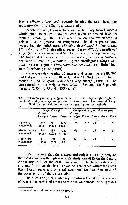
Vegetation samples were harvested in late July from transectswithin each watershed. Samples were taken at ground level toinclude remaining litter. The vegetation on the watersheds isprimarily short grasses and midgrasses. The short grasses andsedges include buffalograss (Buchloe dactyloides),* blue grama[Bouteloua gracilis), threadleaf sedge (Carex filifolia), needleleafsedge (Carex eieocharis), and Sandberg's bluegrass (Ppa secuncla).The midgrasses include western wheatgrass (Agropyron smitlui),ncedle-and-thread (Stipa comata), green needlegrass (Stipa viri-tlula). side-oats grama {Bouteloua curtipendula), and little blue-stem (Andropogon scoparius).

Mean oven-dry weights of grasses and sedges were 819, 364and 404 pounds per acre (918. 408, and 453 kg/ha) from the light-,moderate- and heavy-use watersheds, respectively (Table 1). Thecorresponding litter weights were 2,082, 1,325 and 1,008 poundsper acre (2.334. 1.485 and 1.130 kg/ha).

TAHLF I — Vegetal weight (pounds per acre, oven-dry weight; kg/ha inbrackets) and percentage composition of hasal cover, Cottonwood Range

Field Station, 1967. Values arc the mean of four watersheds.

Vegetal weightCrosses

A sedges Forbs Litter

Composition of basal cover (%)Grasses

<fc sedges Forbs Litter Rock Bare

Light-usewatersheds

819

(918)391

(438)2082

(2334)58 .3 ' 34 1 4

Moderate-usewatersheds

364

(408)183

(205)1325

(1485)65 4 26 0 5

Heavy-usewatersheds

404

(453)60

(67)1008

(1130)68 6 23 1 2

Table 1 shows that the grasses and sedges make up 58% ofthe basal cover on the light-use watersheds and 68% on the heavy.About one-third of the basal cover on the light-use watershedsand one-fourth of the basal cover on the other watersheds waslitter. Forbs, rocks and bare soil accounted for less than 10% ofthe cover on all of the watersheds.

The effects of grazing intensity are also reflected in the speciesof vegetation harvested from the various watersheds. Short grasses

♦ Nomenclature follows Hitchcock (1950).

344

and sedges predominated in the heavy-use watersheds, whilewestern wheatgrass was important in the mixture of grasses onthe light-use watersheds. The long-time effects of grazing intensityreflected a limited amount of midgrasses, such as western wheat-grass, among the predominantly shcrt grasses on the moderate-use areas.

Very little variation in sample weights between the fourreplications on any of the treatments was shown for either theclipping areas or the point line transects.

ANALYSIS OF DATA

To eliminate as much as possible the interaction clfects ofinfiltration estimation upon the determination of watershed-roughness parameters, a storm was chosen wherein rain fell for a totalof nearly II tours. An intense burst of rainfall occurred about9.5 hours after the beginning of rainfall and resulted in an easilyidentified peak rate of runoff. Runoff occurred at all watershedsfor at least 9 hours. Considering the nature of the soils at thesewatersheds, one can assume a constant infiltration rate for the lasthour of the storm. Infiltration rales were computed by assumingthat surface storage at the beginning of the intense portion of rainfall was the same as the storage remaining at the same flow rateduring the recession. Infiltration during this interval was thenthe difference between rainfall and runoff. The infiltration ratescalculated are shown in Table 2.

TABLE 2—Constant infiltration rates during last hour of storm. 15 July1967. Vahies are in inches per hour; mm/min in brackets.)

Treatment /Replication

2 3 4 A verage

Light 0.105

(0.0445)0.109

(0.0462)0.114

(0.0483)0.122

(0.0517)0.113

(0.0480)

Medium 0.080

(0.0338)0.094

(0.0398)0.062

(0.0268)0.052

(0.022)0.072

(0.0305)

Heavy 9.101

(0.0428)0.067

(0.0284)0.079

(0.0335)0.075

(0.0318)0.081

(0.0343)

Lateral inflow rales, q(x,t) as shown in equation (2). wereobtained as step functions in time by subtracting the infiltrationrates in Table 2 from rainfall rales obtained from recording rain

345

gages. These rates became negative when infiltration rates weregreater than runoff rales.

Coitour lmfr»ul 5fl.

FIG. 5—Topographic map and cascade representation of Waterhed H-3Cottonwood, South Dakota. (Scale, 1:2850.)

Watershed geometry was approximated by a series of planesand channels as shown in the example of Figure 5. First the watershed was divided into areas contributing to individual channelsby drawing a stream line upstream from the measuring flume tothe watershed divide. These contributing areas were then subdividedinto rectangular planes to account for slope or width variations.Jhe collecting channels at the lower boundary of the watershedwere constructed by building a low dike on the watershed surfaceThe cross-section of these channels was approximated by a triangular section having I: I side slopes on the dike side and the naturalwatershed slope on the other side.

nf hHT*? W-a! oc.currine from a" watersheds at the beginningof the h.gher-.ntens.ty rainfall period that was used in this studyAsteady-state initial condition was assumed for all planes, wherethe steady-state flow rate was equal to the observed discharge rateat the beginning of the computed event. The channels were assumedto be initially dry.

The parameter k was given an initial value estimated fromprevious studies. When the computations were completed for anevent with the trial value of k, the computed and observed discharges were reduced to rales at uniform 3-mint.te incrementsJhe sum of squares of deviations was then computed and a

346

univariate search technique was used to find the minimum valueof the objective function.

Thus the objective function was

^= / (Qcomp —C?ubs)21=1

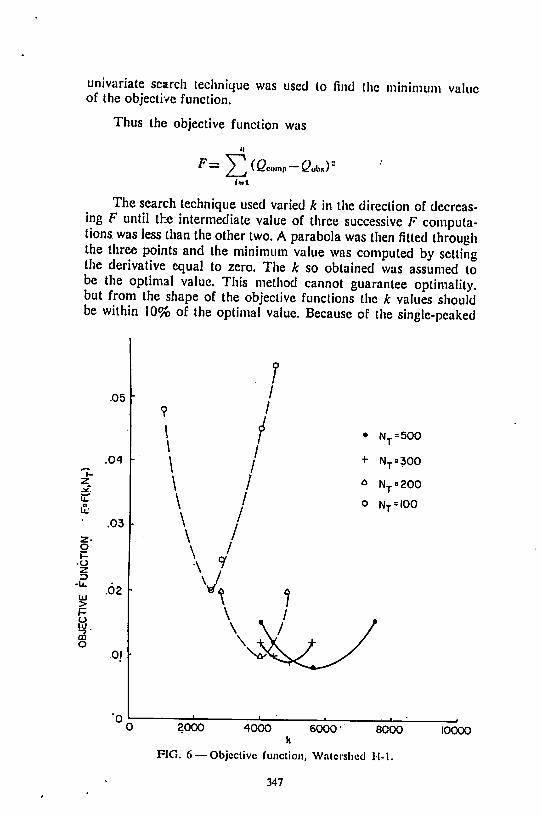
The search technique used varied k in the direction of decreasing F until the intermediate value of three successive F computations was less than the other two. Aparabola was then filled throughthe three points and the minimum value was computed by settingthe derivative equal to zero. The k so obtained was assumed tobe the optimal value. This method cannot guarantee optimality.but from the shape of the objective functions the k values shouldbe within 10% of the optimal value. Because of the single-peaked

• oz

•U.

>

—»

mo

.05

.04

.03

.02

01

• NT=500

+ NT=300

* NT=200

o NT =I00

0 2000 4000 6000- 8000k

FIG. 6 —Objective function, Watershed H-l.

347

10000

shape of the hydrographs, it is extremely unlikely that local minimawould exist.

As the problem has been formulated, the objective functiondepends upon the parameters k and NT or C, where NT is thetransitional Reynolds number. To obtain a single point on theobjective function, the complete hydrograph must be computed.Based upon the observations of previous investigations and anexploration of the bivariate response surface for watersheds H-1and H-4, a transitional Reynolds number of 300 was used in allcalculations. The behaviour of the objective function is shown inFigure 6.

Optimum k values for a transitional Reynolds number of300 were computed for the four heavily grazed watersheds andthe four lightly grazed watersheds. The parameter values obtainedare shown in Table 3. The best and v/orst fits obtained are shownin Figure 7. A Mest indicated that there is no reason to believethat the mean k for the lightly grazed watersheds is different fromthe mean for the heavily grazed watersheds. Because these watersheds have the greatest difference in vegetal cover (see Table 1),it can be inferred that intensity of grazing has no significant effecton hydraulic parameters.

TABLb 3—Optimized parameters for WT=300. Mean-A: for lightly grazedwatersheds 6,029; standard deviation 2,165. Mean k for heavily grazed

watersheds 7,487; standard deviation 3,690.

Hecivily grazed watersheds

L-2 L-3 L-4

Ligl

H-1

illy grazed watershedsL-I H-2 H-3 H-4

k 3932 8919 6495 4769 4875 3761 10518 10793

C 4.43 2.94 3.45 4.03 3.98 4.53 2.71 2.68

F 0.080 0.034 0.068 0.067 0.009 0.008 0.018 0.014

The minimum k value of 3,760 and the maximum of 10,700are both less lhan the respective extremes for turf calculated byMorgali (1970). However, it is quite likely that there are realdifferences between the turf used by Izzard and the short-grassprairie vegetation found on the Cottonwood watersheds.

The / versus NR relationships for this study are shown alongwith Morgali's envelope curves in Figure 8. The range in k is somewhat smaller than was obtained by Morgali, who analyzed repeated

348

i * »

20

Cottonwood, SO.Wolcrshed L-l Event of 6-15-67

• Observed

0 ComputedK'3932

C=4.43

NT=300F= .080

-Lolerol Inflow Rate

40 60

TIME IN MINUTES

FIG. 7(a) —Worst-fitting optimized hydrograph.

80

.05

100

UJ»-

H

2

orUJa

22

experiments on the same material but with varying slopes, lengthand rainfall intensity.

When a fixed transitional Reynolds number is used, theChezy C varies with k according to equation (8). At a steady statecondition with a uniform lateral inflow rate of 0.25 inches per hour(0.106 mm/h), a Reynolds number of 300 would be reached only

349

z

z

<

o

Cottonwood, S .0.Watershed H-1, Event of 6-15-67

• Observed

o Ccmpuled

Lateral InflowRate-

20 <\0 eo

TIME IN MINUTES

80

K*4B75C*3.98

NT=300F-.009

•8

100

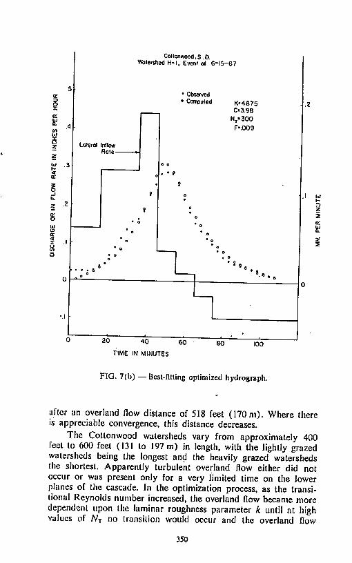
FIG. 7(b) — Best-fitting optimized hydrograph.

.1 iu

after an overland flow distance of 518 feet (170m). Where thereis appreciable convergence, this distance decreases.

The Coltonwood watersheds vary from approximately 400feel to 600 feel (131 to 197m) in length, with the lightly grazedwatersheds being the longest and the heavily grazed watershedsthe shortest. Apparently turbulent overland flow either did notoccur or was present only for a very limited time on the lowerplanes of the cascade. Jn the optimization process, as the transitional Reynolds number increased, the overland flow became moredependent upon the laminar roughness parameter k until at highvalues of /VT no transition would occur and the overland flow

350

hydrograph would depend only upon k. The friction factor forthe channelswas assumed to be equal to that for turbulent overlandflow so as /VT increased, the channel friction factor decreased andthe channels began to influence the outflow hydrograph. It wasnoted, Jiowever, that in most cases the channel did very little morethan lag the overland flow hydrograph by approximately two orthree minutes.

K>,000

FIG. 8 — Darcy-Weisbach / versus Reynolds number.

As a test of the predictive capability of the mathematicalmodel, hydrographs were computed for the four moderately grazedwatersheds for the same storm with the parameter k set equalto the mean of the optimized k values for the lightly and heavilygrazed watersheds. The best-fitting and the worst-fitting hydro-graphs are shown in Figure 9 and a tabulation of objective functionvalues, F, and a comparison of observed and computed peak ratesare shown in Table 4.

351

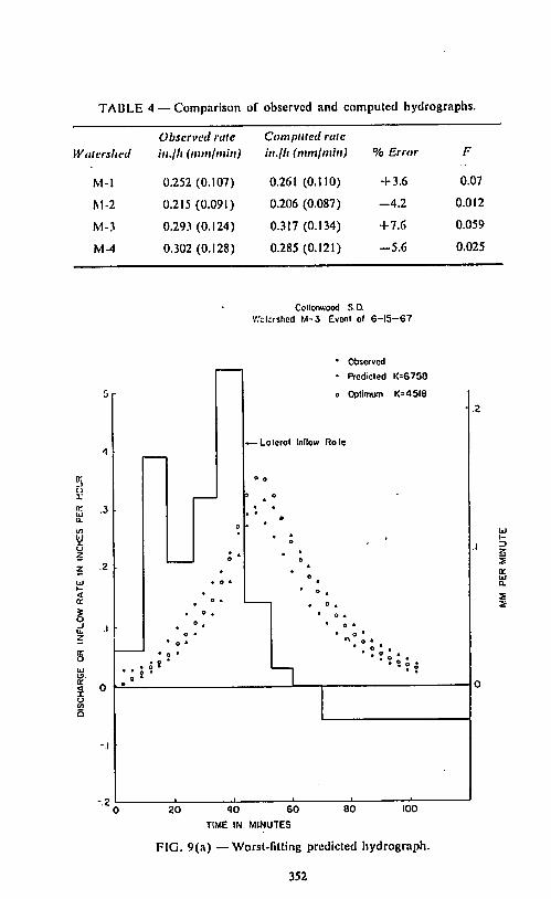
TABLE 4 — Comparison of observed and computed hydrographs.

Watershed

Observed rale

in./h (mm/min)

Computed ralein.Ih (mmjmin) % Error F

M-l 0.252 (0.107) 0.261 (0.110) + 3.6 0.07

M-2 0.215(0.091) 0.206 (0.087) -4.2 0.012

M-3 0.293 (0.124) 0.317 (0.134) +7.6 0.059

lvi-4 0.302 (0.128) 0.285(0.121) -5.6 0.025

• Cottonwood SO.

Wclcrshcd M-3 Event of 6-15-67

• Observed

- Predicted K=67G0

0 o Optimum K*45I8

— Loterol Inflow Role

•

<*.

o o

» o

.3

0

o

a

o . '

o

0

.2

« o »

. * o ,o •

•

• O 4 • o •

t .

0 . • o *

• o »• o *

•V o •• . o * .

• • <a *

• o *

5* ' •'si:.0

-.1

- 0

20 40 60

TIME IN MINUTES

80 100

FIG. 9(a) —Worst-fitting predicted hydrograph.

352

orr>oX

rrUJ

5f

2 .2tu

or

Cottonwood, S.D.Watershed M-2 Event of 6-15-67

• Observed

* Predicted

nk*6758

-Lateral Inflow Role

J

» « M ' • *

-.2

20 40 60 80

TIME IN MINUTES

FIG. 9(b) —Best-fitting predicted hydrograph.

100

.2

Z32

2

rr

52

The observed and computed hydrographs agree very wellBecause these watersheds were not used to estimate the roughnessparameters, this prediction suggests that the kinematic cascadeis an acceptable model for overland flow on watersheds of this

353

size, and that the roughness parameters might be used in otherareas with similar topography and vegetal characteristics.

DISCUSSION OF SOURCES OF ERROR

As in any empirical study, several sources of error were presentthat undoubtedly have some eflect on the magnitude and variabilityof the roughness parameters obtained by the optimization procedure. During the time of the runoff event, the rain gages and water-stage recorders were serviced by an inexperienced operator whodid not annotate the charts properly. Ordinarily, synchronizationerrors between precipitation measurements and runoff measurements would be on the order of ±5 minutes. For this storm, timingerrors could be as large as ±10 minutes. As an indication of thesensitivity of the parameter k to errors in synchronization betweenrainfall and runoff records, an optimization calculation was madefor watershed H-2 with the observed hydrograph lagged 10minutes. The optimum k obtained was 11,660 as compared with3.761 without the time shift. The variability in the k values forthe heavily grazed watershed can easily be accounted for bysynchronization errors. The assumption of a constant infiltrationrale during the last part of the storm is probably not a source ofsignificant error. The errors in estimating rainfall rales are probablynot serious because recording rain gages were located adjacentto each group of watersheds. The rates are subject to ordinaryinstrumental error and the variability due to numerically differentiating the cumulative rainfall curve.

The assumption of a steady-slate overland flow profile as aninitial condition probably overestimates the amount of initial storageand would tend to increase the optimum k. A correlation betweenthe optimum k values and the magnitude of the initial flow ratewas observed, with the higher k values associated with high initialflow rates.

Finally, the flow rates are subject to flume-rating errors whichmay be on the order of 3% if the water-stage recorder is carefullyadjusted. If the gage is not zeroed properly, the records will bebiased. At the peak flow rates observed during this storm, a zero-reading error of 0.01 foot would introduce an error of approximately 4%.

SUMMARY AND CONCLUSIONS

The kinematic cascade was used as a mathematical model

to describe overland and open-channel flow for small rangelandwatersheds. Optimum roughness parameters were computed for

354

four heavily grazed watersheds and four lightly grazed watershedsfor a single storm. Although these watersheds showed substantialdifferences in vegetal composition and cover in weight of vegetationper unit area, the roughness parameters for the lightly grazed watersheds were not significantly greater than for the heavily grazedwatersheds.

The average of the eight roughness parameters was used inthe kinematic-cascade model to predict runolt hydrographs for fourmoderately grazed watersheds with very good results.

The following conclusion can be drawn from this study:(1) The kinematic-cascade model can accurately describe the

outflow hydrograph for small watersheds with predominantly overland flow.

(2) The roughness parameter, k, in the laminar frictionrelationship f=k/NR is approximately 7,000 for short-grass prairiewatersheds if the transitional Reynolds number is 300.

(3) The friction parameters obtained by the methods usedin this study are consistent with those obtained by analysis oflaboratory data.

(4) It wculd be desirable to make a similar analysis for otherstorms where timing errors would be small. The response of theobjectiive function to variations in the transitional Reynolds numbershould be explored for all watersheds.

REFERENCES

Chow, V. T. 1959: Open Channel Hydraulics. McGraw-Hill, New York.

Das, K. C; Hu^ins, L. F. 1970: Laboratory Modeling and Overland FlowAnalysts. Purdue University Water Resources Research Center.Lafayette, Indiana. 182p.

Henderson, F. M.; Wooding, R. A. 1964: Overland flow and groundwaterflow frcjn a steady rainfall of finite duration. J. Gcophys. Res. 69(8): 1531-1540.

Hitchcock, A. S. 1950: Manual of the grasses of the United States. 2nd cd.(revisec by Agnes Chase). USDA Misc. Pub. 200. 1051 p.

Izzard, C. F. 1942-43: Overland Flow Tests— Tabulated Hydrographs.vol. 1-3. U.S. Bureau of Public Roads, (available' from theEngineering Societies Library.)

Kibler, D. F.; Woolhiser, D. A. 1970: The kinematic cascade as a hydro-logic model. Colorado State University Hydrology Paper No. 39.27 p.

355

Lewis, J. K.; Van Dyne, G. M.; Albee, L. R.; Whetzal, F. W. 1956.Intensity of grazing — its effect on livestock and forage production.South Dakota Agr. Exp. Sta. Bull. 459. Brookings, S.D. 44 p.

Lighthill, M. J.; Whitham, G. B. 1955: On kinematic waves. I. Flood movement in long rivers. Proc. Roy. Soc. London (A) 229: 281-316.

Morgali, J. R. 1970: Laminar and turbulent overland flow. Proc. ASCE96 (HY2): 441-460.

Schaake, J. C. 1965: Synthesis of the inlet hydrograph. The Storm DrainageResearch Project, Tech. Report No. 3. John Hopkins University.

Spuhlcr, W.; Lytic, W. F.; Moe, D. 1968: Climatological Summary No. 14,Climatography of the U.S. No. 20-39. (from U.S. Weather Bureaurecords.)

Wcslin, F. C; Puhr, L. F.; Buntlcy, G. J. 1967: Soils of South Dakota.Soil Survey Series No. 3. South Dakota Agr. Exp. Sta., Brookings,S.D. 32 p.

Woo, D.-C; Bralcr, E. F. 1962: Spatially varied flow from controlled rainfall. Proc. ASCE 88 (HY6) : 31-56.

Wooding. R. A. 1965: A hydraulic model fcr the catchment-stream problem.•• I. Kinematic wave theory. Journ. Hydrol. (Neth.) 3: 254-267.

Yu, Y. S.; McNown, J. S. 1964: Runoff from impervious surfaces. Journ.Hydraulic Research 2 (1): 3-24.

356