University of KentuckyUKnowledge

KWRRI Research Reports Kentucky Water Resources Research Institute

8-1985

Modeling of Overland Flow by the Diffusion WaveApproachDigital Object Identifier: https://doi.org/10.13023/kwrri.rr.159

Rao S. GovindarajuUniversity of Kentucky

S. E. JonesUniversity of Kentucky

M. L. KavvasUniversity of Kentucky

Right click to open a feedback form in a new tab to let us know how this document benefits you.

Follow this and additional works at: https://uknowledge.uky.edu/kwrri_reports

Part of the Hydrology Commons, Oil, Gas, and Energy Commons, and the Water ResourceManagement Commons

This Report is brought to you for free and open access by the Kentucky Water Resources Research Institute at UKnowledge. It has been accepted forinclusion in KWRRI Research Reports by an authorized administrator of UKnowledge. For more information, please contactUKnowledge@lsv.uky.edu.

Repository CitationGovindaraju, Rao S.; Jones, S. E.; and Kavvas, M. L., "Modeling of Overland Flow by the Diffusion Wave Approach" (1985). KWRRIResearch Reports. 45.https://uknowledge.uky.edu/kwrri_reports/45

Research Report No. 159

MODELING OF OVERLAND FLOW BY THE DIFFUSION WAVE APPROACH

By

Rao S. Govindaraju Graduate Assistant

S.E. Jones Investigator

M. i.. Kavvas Principal Investigator

Project Number: G-908-03 (A-098-KY)

Agreement Numbers: 14-08-0001-G-908 (FY 1984)

Period of Project: July 1984 - August 1985

Water Resources Research Institute University of Kentucky

Lexington, Kentucky

The work upon which this report is based was supported in part by funds provided by the United States Department of the Interior, Washington, D.C., as authorized by the Water Research and Development Act of 1984, Public Law 98-146

August 1985

DISCLAIMER

Contents of this report do not necessarily reflect the

views and policies of the United States Department of the

Interior, Washington, D.C., nor does any mention of trade

names or commercial products constitute their endorsement or

recommendation for use by the U.S. Government.

ii

-

ABSTRACT

MODELING OF OVERLAND FLOW BY THE DIFFUSION WAVE APPROACH

One of the major issues of present times, i.e. water quality degradation and a need for precise answers to transport of pollutants by overland flow, is addressed with special reference to the evaporator pits located adjacent to streams in the oil-producing regions of Eastern Kentucky. The practical shortcomings of the state-of-the-art kinematic wave are discussed and a new mathematical modeling-approach for overland flows using the more comprehensive diffusion wave is attempted as the first step in solving this problem. A Fourier series representation of the solution to the diffusion wave is adopted and found to perform well. The physically justified boundary conditions for steep slopes is considered and both numerical and analytical schemes are developed. The zero-depth-gradient lower condition is used and found to be adequate. The steady state analysis for mild slopes is found to be informative and both analytical and numerical solutions are found. The effect of imposing transients on the steady state solution are considered. Finally the cases for which these techniques can be used are presented.

Descriptors: Model Studies, Overland Flow, Oil Fields, Oily Pollution, Flow Characteristics, Flow Pattern

iii

ACKNOWLEDGEMENTS

The research work that led to this thesis was funded by

U.S. Dept. of the Interior through U.S.G.S. and KWRII. This

support is gratefully acknowledged. Special thanks are due

Beverly ~ullins for patiently typing the equations.

lV

TITLE PAGE

DISCLAIMER

ABSTRACT

ACKNOWLEDGEMENTS

TABLE OF CONTENTS

LIST OF TABLES

LIST OF ILLUSTRATIONS

TABLE OF CONTENTS

CHAPTER 1 - INTRODUCTION

1.1 Motivation for the Project

1.2

1.3

1.4

Framework of the Report

Survey of some previous Work

Project Objectives

CHAPTER 2 - SOLUTION FOR STEEP SLOPES

2.1 Description

2.2 Theory of the Numerical Series Solution

2.3 Theory of the Analytical Solution

2.4 Performance of the Series Solution Scheme

CHAPTER 3 - ANALYSIS OF THE STEADY STATE

3.1 Description

3.2 The Steady State Theory

Page

i

ii

iii

iv

v

vi

vii

1

3

5

31

33

34

37

49

54

55

3.3 The Numerical Steady State Solution 56

3.4 Analytical Approximations to the Steady State 57

3.5 Transient Solutions 64

v

CHAPTER 4 - DISCUSSION AND CONCLUSIONS

4.1 Discussion

4.2 Conclusions

NOMENCLATURE

REFERENCES

APPENDIX Reference for Outflow Profiles

Table

2.1

LIST OF TABLES

Table showing steady state values

for two-term analytical solution

vi

69

71

75

77

79

Page

51

Figure

1.1

l • 2

1.3

l.4a,b

2.2.a-d

2.2e-h

2.2i,j

2.3a-d

2.3e,f

3.3a-f

3.4a-f

3.Sa-d

LIST OF ILLUSTRATIONS

Overland flow

Definition sketch of overland flow

Zones in the (x,t) plane

Zones of the Fo, K field

Rising outflow hydrographs for 2-term

numerical series solution

Rising outflow hydrographs for 3-term

numerical series solution

Recession outflow hydrographs for 3-term

numerical series solution

Rising outflow hydrograph for 2-term

analytical series solution

Recession outflow hydrograph for 2-term

analytical series solution

Steady state profiles for the zero­

depth-gradient downstream boundary

condition

Steady state profiles for critical

flow downstream boundary condition

Rising outflow hydrograph for 1-term

numerical series solution for zero-

vii

Page

6

11

16

30

38

40

42

46

48

58

61

Figure

3,5e,f

LIST OF ILLUSTRATIONS (CONTND.)

depth-gradient condition

Recession outflow hydrograph for I-term

numerical series solution for the zero­

depth-gradient condition

viii

Page

66

68

CHAPTER .L_ INTRODUCTION

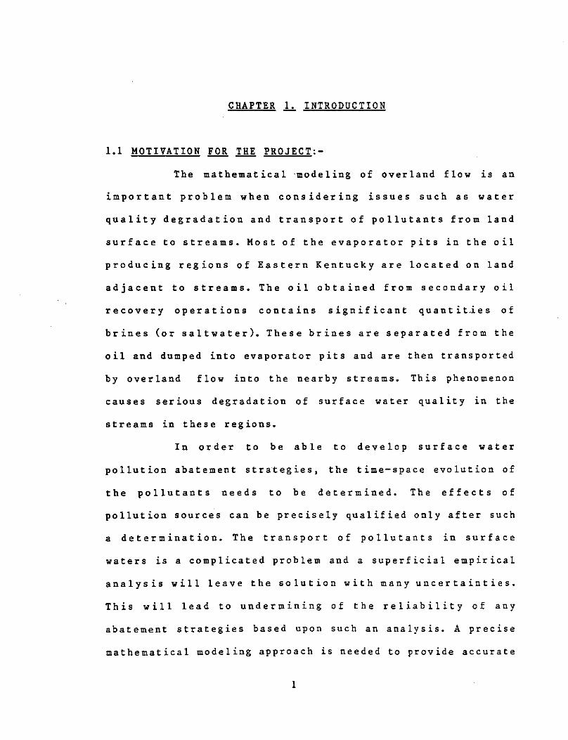
1.1 MOTIVATION FOR THE PROJECT:-

The mathematical ·modeling of overland flow is an

important problem when considering issues such as water

quality degradation and transport of pollutants from land

surface to streams. Most of the evaporator pits in the oil

producing regions of Eastern Kentucky are located on land

adjacent to streams. The oil obtained from secondary oil

recovery operations contains significant quantit.ies of

brines (or saltwater). These brines are separated from the

oil and dumped into evaporator pits and are then transported

by overland flow into the nearby streams. This phenomenon

causes serious degradation of surface water quality in the

streams in these regions.

In order to be able to develop surface water

pollution abatement strategies, the time-space evolution of

the pollutants needs to be determined. The effects of

pollution sources can be precisely qualified only after such

a determination. The transport of pollutants in surface

waters is a complicated problem and a superficial empirical

analysis will leave the solution with many uncertainties,

This will lead to undermining of the reliability of any

abatement strategies based upon such an analysis. A precise

mathematical modeling approach is needed to provide accurate

1

numerical answers to the time-space evolution of pollutants

in surface waters.

The transport process of pollutants by surface

waters can be separated into the overland flow and the

channel flow phases. The first phase of transfer through

overland flow carries the pollutant from land surface to

neighbouring streams as in the evaporator pits of Eastern

Kentucky's oil producing regions. In order to solve this

problem one needs to know the flow depth h(x,t) and the

discharge per unit width q(x,t) over the flow domain. This

study will provide approximate analytical solutions to the

hydraulic problem of flow using the diffusion wave

approximation. The state-of-the-art approach to the overland

flow modeling is the kinematic wave. The practical

shortcomings of this method are discussed and the more

comprehensive diffusion wave is used for the purposes of

this study. The solutions obtained will provide the

requisite depth and discharge values over the overland flow

domain under realistic initial and end conditions.

The problem attempted in this report is of a very

fundamental nature and therefore has application in many

larger problems. It is a small element when considering

catchment-stream problems. The equations of channel flow are

of similar nature and the concepts developed during this

study may be extended to solve the equations governing such

flows. Thus it may be possible to obtain analytical (or

semi-analytical) solutions for flood propagation in channels

2

and new solutions to flows in channel networks. These

networks may be looked upon as a collection of overland flow

reaches and converging sections interlaced by channels. The

problem under consideration is a simpler version of the two

dimensional overland flow and thus needs to be solved before

attempting the more difficult case.

1.2 FRAMEWORK OF THE REPORT:-

This report presents a new solution to the

diffusion wave equation under some acceptable initial and

end conditions. It has been presumed that the wave profile

is made up of many components which when properly

superimposed together sum up to the true wave form. A

Fourier series representation to the solution has been found

to be most appropriate for this purpose and has been adopted

for a major part of this study.

The present chapter considers the justification of

such an effort. Pollution transport, flood waves, channel

networks, two-dimensional overland flows are some of the

benefits to be derived from this solution. This chapter also

states the objectives and aims of the project. A brief

review of past work directly connected with the problem of

interest has also been included. A critical appraisal of the

methods adopted by previous researchers and their relative

merits and demerits have been discussed.

The second section deals with the solution to the

flow equation when applied to steep slopes. The associated

end conditions and numerical and analytical solutions of the

3

resulting system have been developed. A sine series solution

has been found to be very effective numerically and many

ca_ses have been demonstrated to show its performance (Fig.

2.2). The analytical solution for this case reduces to an

eigenvalue problem after effecting a simple Taylor series

expansion. The resulting solution is found to be good near

the steady state and a similar procedure adopted for the

recession region has been found to give reasonable results

(see Fig. 2.3).

The solution for mild slopes is dealt with in the

third chapter. The solution is split up into two components;

a steady state solution and transient solution•. The

complete· solution is obtained when sufficient number of

transients are added on the steady state,

dictated by the accuracy desired by the

this number being

user. The steady

state numerical solutions are presented for the diffusion

wave (Fig. 3.4). The effect of adding one term transient on

to the steady state solution is considered for the zero­

depth-gradient downstream boundary condition (Fig. 3.5).

Analytical solutions for the steady state for this case are

considered in the form of polynomials (Fig. 3.3). The

numerical solution to the steady state for critical flow

downstream condition is also presented (Fig. 3.4).

The last chapter presents a global picture of the

report and states the conditions under which any particular

approximation may be used. Important conclusions regarding

the accuracy and justification of these solutions are

4

presented. The consequences of this solution procedure are

stated. Results obtained by other investigators have also

been included in the figures for comparison purposes.

References for these are given in the Appendix.

1.3 SURVEY OF PREVIOUS WORK:-

It is known from literature that the flow in open

channels is governed by the gradually varied, unsteady,one

dimensional shallow water equations known as Saint- Venant

equations (see, for example, Vieira [1982]). These are given

by equations (1.1) and (1.2). The flow is one dimensional in

the x- direction, t is the time, his the depth, u is the

average velocity at (x,t) and q is the lateral inflow per

unit area per unit time.

The continuity equation, then, for unit width of plane is:

( 1.1 )

and the momentum equation is:

~ + u ~ + g cose 2.h. - g(sine - Sf) - ~hu at ax ax ( 1. 2 )

where g is the acceleration due to gravity; e the angle of

the slope, assumed constant; and oghSf = the frictional

retarding force exerted by the plane on the water. Sf is

usually defined by the Chezy equation:

( 1. 3 )

C being the Chezy roughness of the plane. In the case of

overland flow q is the rainfall plus any seepage less any

5

infiltration from the ground

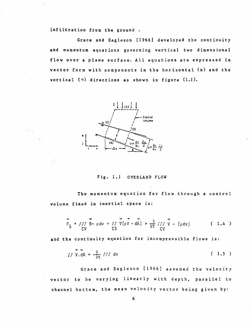
Grace and Eagleson [1966] developed the continuity

and momentum equations governing vertical two dimensional

flow over a plane surface. All equations are expressed in

vector form with components in the horizontal (x) and the

vertical ( 11) directions as shown in figure (1.1).

'

Fig. 1.1 OVERLAND FLOW

The momentum equation for flow through a control

volume fixed in inertial space is:

.... F S + ! ! ! B • p dv

CV

... ... ... = ! ! V (p V • dA) + a~

cs

.... ffj V • (pdv)

CV ( 1.4

and the continuity equation for incompressible flows is:

....... If V.dA

a = -- ff f dv at

( 1. 5

)

)

Grace and Eagleson [1966] assumed the velocity

vector to be varying linearly with depth, parallel to

channel bottom, the mean velocity vector being given by:

6

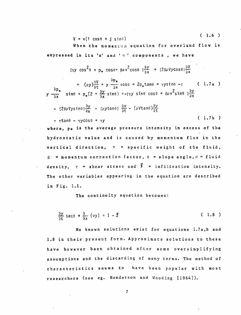
V = v(i cose + j sin8) ( 1. 6 )

When the momentu~ equation for overland flow is

expressed in its 'x' and 'ri ' components , we have

[yy cos 2e + p* cose-1- ~pv2cose 11f + [2SpVycoseJ !~ av ap. .

(py)-t + y - case = 2p*tane + yys,na --r a ax + ( 1. 7 a )

sine + ( av . ) . 2 . e 1.£.l. p* 2 +~sine =-[yy sine cose + BPV sin ax

[28pVysin8J~ - [pytaneJ !~ - (pVtanel-ff-

- ,tans - yycose + yy ( l.7b )

where, P* is the average pressure intensity in excess of the

hydrostatic value and is caused by momentum flux in the

vertical direction, Y = specific weight of the fluid,

I',- = momentum correction factor, 8 = slope angle, P = fluid

density, = shear stress and ~ = infiltration intensity.

The other variables appearing in the equation are described

in Fig. 1.1.

The continuity equation becomes:

tf sece + :x (vy) = I -S ( 1.8 )

No known solutions exist for equations l.7a,b and

1.8 in their present form. Approximate solutions to these

have however been obtained after some oversimplifying

assumptions and the discarding of many terms. The method of

characteristics seems to have been popular with most

researchers (see eg. Henderson and Wooding (1964]).

7

Grace and Eagleson have carried out a systematic

study of the orders of magnitude of the terms appearing in

equations l.7a and l.7b. This then provides physically

justifiable reasons for discarding or retaining a term.

Normalization of these dimensional equations was then

carried out by defining dimensionless ratios linking all

variables with appropriate reference variables. A similar

analysis was carried out on the non dimensional equations,

In the process of carrying out an 'Order of Magnitude

Analysis' the following assumptions were made

1) Surface tension effects are negligible in

both model and prototype.

2) Roll wave formation, if present is

dynamically similar in model and yrototype.

3) There is no infiltration in the model.

4) Dep,th to length ratio of the model, 1.e.

(Y/L) should be less than 0.003.

5) Slope of the bed surface of the model

should be greater than 5 degrees,

where cf

6) For both prototype and model overland flow

cf ta ne < < 4,

is the non dimensional frictional coefficient,

7) The overland flow is two dimensional,

It may be noted that l,7a and l.7b are the most

general forms of these equations, The expression for the

dimensionless over-pressure term p* may be obtained from the

non dimensional form of the momentum equation in

8

the n direction ( obtained from l.7b ), From the 'Order of

Magnitude Analysis' presented by Grace and Eagleson it

follows that all terms regarding rainfall, infiltration and

Y/L may be neglected in the expression for the over-pressure

for the prototype in case of steep bed slopes, A similar

analysis for the model gives an expression for the

normalized over-pressure which is identical to the one

obtained for the prototype, For reasonable modelling, the

model slope should be greater than 5° to include the

frictional and gravitational effects. This expression for

the over-pressure term may be substituted into the

dimensionless momentum equation in the x direction obtained

from l.7a. Then for small slopes and for B = l ( where

B = momentum correction factor ) the commonly used momentum

equation may be obtained after some further simplification.

Finite difference solutions adopting various

schemes for solving the differential equations were

investigated. Woolhiser and Liggett [1967] considered the

acceptable numerical methods which can be used in connection

with shallow water equations primarily with overland flow

applications, Their study provides suitable guidelines for

choosing stable finite difference schemes, For small values

of e, i.e. for mild slopes, (1.1) and (1.2) may be written

as

ah + 11 ah + h ~ = q at -ax at

( 1. 9 )

9

( 1.10 )

where s0 is the sine of the slope angle for small slopes.

The shallow water equations can be treated more generally by

adopting a dimensionless representation. Then

v2 s = 0 O C2H

0

( 1.11 )

in which, Ho= normal flow depth for flow Qo = qLo at the

end of the reach under consideration (at x = Lo); Vo is the

normal velocity for Qo = qLo at x = Lo· When the flow in the

reach of length Lo comes in as lateral inflow q,

( 1.12 )

The quantities Ho, v0 and Lo are frequently used as

normalizing constants and the following dimensionless

variables are defined:

u* = u h*

h x VO ; =

Ha x* =- t* = tr-VO La 0 ( 1.13 )

Also we have,

Fa VO

k Solo

=-- = F2 VgH0 HO 0

( 1.14 )

Then the dimensionless shallow water equations are:

( 1.1 5 )

( 1.16 )

10

The dimensionless lateral inflow, is obtained by

dividing the lateral inflow by the maximum rate, qmax· It is

worth noting that the dimensionless time is related to the

'time of equilibrium', a t* value of 1.0 being the time

required for a fluid particle to traverse the reach under

the normal flow conditions. The dimensionless flow equations

have only two parameters F 0 and K (excluding R) instead of

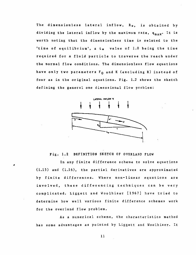
four as in the original equations. Fig. 1.2 shows the sketch

defining the general one dimensional flow problem:

UTERAL INF\..CW Cl

Fig. 1.2 DEFINITION SKETCH OF OVERLAND FLOW

In any finite difference scheme to solve equations

(1.15) and (1.16), the partial derivatives are approximated

by finite differences. Where non-linear equations are

involved, these differencing techniques can be very

complicated. Liggett and Woolhiser [ 1967] have tried to

determine how well various finite difference schemes work

for the overland flow problem.

As a nl,\merical scheme, the characteristics method

has some advantages as pointed by Liggett and Woolhiser. It

11

is accurate because the characteristics trace the path of

the disturbances, The characteristics have an adaptive

property i.e. they tend to be closer together in areas of

rapid change. The method of characteristics is also

reasonably fast and for a given accuracy criteria it covers

maximum ground on the x-t plane. Yet another advantage is

that it does not have to face the 'starting problem'. The

usual initial condition of dry surface often leads to

singularities which create certain difficulties. However,

it suffers from the chief disadvantage of not having a

uniform mesh spacing. A special interpolation subroutine

needs to be incorporated which consumes time of both man and

machine, not to mention the extra large high speed memory

space required to handle medium sized problems.

Explicit methods refer to those finite difference

schemes where the results at any time step may be explicitly

obtained using values from previous time steps.

Unfortunately, in non-linear partial differential

equations, precise stability criteria can rarely be found.

It was commonly agreed among investigators that the Courant

condition

~! ( I u I + cl ~ 1 ( 1.17 )

is a necessary condition for stability of an explicit finite

difference scheme. However it is by no means sufficient, In

general explicit methods are unsatisfactory for even very

approximate calculations.

12

Implicit Method is usually a safe method and

involves solving a set of simultaneous equations for each

row of points at every time step. Centered differencing is

used to ensure stability. Newton's method is commonly used

for solving the non-linear system of equations. The user is

left with the onus of prescribing an initial guess.

Therefore prior knowledge as to the behaviour of the

solution must be known to the user. A 'double sweep

method' which requires only a 2 by 2 matrix inversion and is

very efficient has been suggested. This method was

subsequently used by other investigators in their work (e.g.

Morris [1980]). Liggett and Woolhiser [1967] have made a

study into the various methods and presented them in a

tabular form.

Amein [1968] considered the need for a fast (i.e.

rapidly convergent) and accurate method for numerical

solutions of unsteady flows. He evolved such a method

consisting of a centered finite difference scheme and

solving the resulting system of non-linear simultaneous

equations by the generalized Newton's method.

To illustrate the validity of his method, Amein

solved a problem originally considered by some other

researchers. He has presented an excellent comparison with

three different methods viz. storage routing equation,

explicit method and method of characteristics. It was seen

that the solutions of the problems obtained by the direct

implicit method are in very good agreement with the best

13

results (i.e. when smallest time steps are used) of the

characteristics method and are quite close to the results

obtained from the explicit method. He also observed that the

linear system of simultaneous equations (arising from

Ne~ton's method) has very few non zero elements, and that

these are clustered around the diagonal. This property of

the matrix can be exploited for fast solutions.

It was soon realized that the complete Saint-

Venant equations are too complex to be solved analytically.

Hence, since the early sixties hydrologists have tried to

obtain physically justifiable approximations which are

easier to handle and operate. Lighthill and Whitham (1955]

have considered a class of wave motions which are physically

quite distinct from the classical wave motions encountered

in dynamical systems, They stated that the kinematic waves

possessed one wave velocity at each point because of the

conservation law or the continuity equation:

( 1.18 )

where, q is the flow quantity passing a given point in unit

time and k is the concentration (i.e. quantity per unit

distance). Kinematic waves are non dispersive but they may

change form due to non linearity (i.e. wave velocity, c,

depends on q). Hence continuous wave forms may develop

discontinuities due to faster waves overtaking slower ones,

These are called shock waves. The properties of such shock

14

'waves have been described. A detailed treatment of flood

movement in long rivers is then considered where kinematic

waves play a leading· role. It is the contention of the

authors that the dynamic waves are rapidly attenuated and

the main disturbances are then carried downstream by

kinematic waves. It was found that if (J/2)Vo and

are taken as typical wave velocities for kinematic

and dynamic waves respectively, then F = 2 (where F is the

Froude number v0

J/gh0

) is the value at which these

velocities are approximately equal. It appears that

kinematic conditions prevail and dynamic effects die out

exponentially when F < 1 (subcritical flows). For F > .2, the

approximate theory ceases to apply. For subcritical flow

case the equations were further 1 in ear ized and it was

noticed that the complete solution contains both kinematic

and dynamic wave fronts.

In 1964, Henderson and Wooding developed the

kinematic wave approximation to the equations of overland

flow on a plane. This involves significant simplification in

the momentum equation where the friction slope is considered

equal to the bed slope and all other terms are neglected. An

analytical solution to the kinematic wave model for overland

flow on a sloping plane was obtained by them. However their

analytical solution was valid only for constant rainfall and

constant infiltration in time and space. Further, they did

not specify any lower boundary condition to the stream.

In a comprehensive treatment of overland flow on a

15

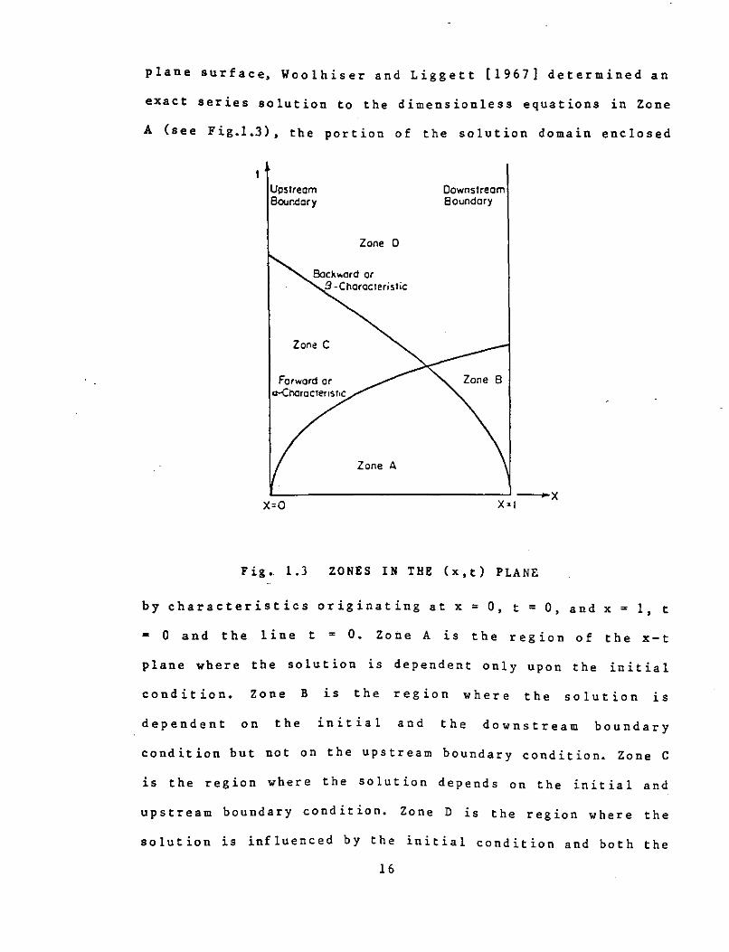
plane surface, Woolhiser and Liggett [1967] determined an

exact series solution to the dimensionless equations in Zone

A (see Fig.l.J), the portion of the solution domain enclosed

Upstream Bour.dory

Zone D

Zone A

Downstream Boundary

L..------------------------------~------x X=O X=I

Fig •. 1.3 ZONES IN THE (x,t) PLANE

by characteristics originating at x = 0, t = 0, and x = 1, t

= 0 and the line t = 0. Zone A is the region of the x-t

plane where the solution is dependent only upon the initial

condition. Zone Bis the region where the solution is

dependent on the initial and the downstream boundary

condition but not on the upstream boundary condition. Zone C

is the region where the solution depends on the initial and

upstream boundary condition, Zone D is the region where the

solution is influenced by the initial condition and both the

16

boundary conditions,

Woolhiser and Liggett [1967] considered an

algebraic approximation t'o the series solution for the

velocity of flow and the possible error involved in adopting

such a technique, Normal depth normalizing was adopted for

non dimensionalising the shallow water equations where the

lateral inflow was represented by a step function, However

for very small values of Fo = vn/ vgH (Froude number for ,, n

normal flow at x* =l), critical depth normalizing was used,

They obtained most numerical solutions by the method of

characteristics described earlier, For very large values of

K (= S0

L0

I H0F~) many difficulties arose with the numerical

integration, The problem was reformulated and solved. It was

noticed that the outflow hydrograph rises as t*3/2 until

equilibrium is reached and then remains f 1 at,

The difficulties in solving equations (1.15) and

(1.16) for large Kare in part associated with boundary

conditions. The problem was clearly defined including all

boundary conditions and approximations by Vieira [1983] and

appears later in the text (see page 25). It was noticed that

supercritical flows have numerical difficulties at upstream

boundary while the numerical integration rapidly lost

accuracy at the downstream end for subcritical flows,

Woolhiser and Liggett have solved for the intersection point

of the characteristics beginning at (0,0) and x* = 1, t* = 0

-the time of intersection of these characteristics can be

found by setting \, = \, and was found to be dependant only

17

on Fo and R:

F 2/3 T = ( 3/ 4 _Q_ ) .

aB ,.,--;f ( 1.19 )

where a and B represent the forward and backward

ch~racteristics respectively (see Fig.1.4).

The variation of Zone A domain with changes in Fo

and were clearly demonstrated in a graph by

Woolhiser and Liggett. The effect of the dimensionless

parameters Fo and K on the rising hydrographs were studied

by them and the results compared with those obtained by

previous investigators. They concluded that there is no

single unique dimensionless rising hydrograph. Also as K

becomes larger the hydrographs are independent of F 0 and

approach the case for Ks infinite. This case corresponds to

the kinematic solution given by Henderson and Wooding

[1964]. Woolhiser and Liggett concluded that the kinematic

wave approximates most physical cases. No recession cases

were considered till later by Morris [1978].

An exact analytical solution to the full Saint-

Venant equations describing flow over a plane on a wide

channel with general turbulent friction was obtained by

Brutsaert [1968]. His solution is applicable only to Zone A.

The lateral ·inflow was assumed uniform. He concluded that

for very large slopes or for a large roughness of the plane,

the solution reduces to the one obtained using the Kinematic

Wave approximation.

Woolhiser [1974] considered the kinematic

18

approximation and the effects of varying and Kon the

rising portion of the hydrographs. He stated that the

kinematic model is a gross simplification of the momentum

equation (1.2). In fact, the kinematic wave yields

analytical solutions only for rainfall rate independent of

any space or time variation and when very simple geometries

are being taken into consideration. These solutions give an

insight into the problem. Care must be taken while modelling

flows using this approach since it is incapable of

accounting for backwater effects. Woolhiser has further

looked into the friction factors and hydraulic resistance

offered to overland flow - especially those arising from

boundary roughness. He presented a very informative table

containing the resistance parameters for overland flows

giving values of laminar resistance, Ko, Manning's

coefficient T) and Chezy's C for typical surfaces. It has

been observed that the effect of impact of raindrops may

have non-negligible effect on flows. Since incorporating

this 'over-pressure' term directly into the equations

governing flows makes them too complicated, their effects

may be introduced by a judicious control over the friction

factor coefficients. Hydrologic applications include

modeling real life problems; the first step of which is to

decide upon the model geometry. An example of geometric

simplification, involving maintaining a close geometric

similarity between prototype watershed and the idealized

network or cascade of planes and channels that specify the

19

model geometry has been considered by Woolhiser [1974]. He

concluded that the Kinematic approximation is good enough

for most urban and rural watersheds.

Morris [1978] considered a new implicit finite

difference method for the solution of the equations (1.1)

and (1.2). The method described uses central differencing

for inside points and backward and forward differencing for

upstream and downstream boundaries respectively. The double

sweep algorithm adopted from Richtmyer's method was used

(see also Liggett and Woolhiser [1967]). Morris introduced

the zero-depth-gradient condition for subcritical flows.

Using this downstream boundary condition she was able to

obtain stable results for cases where the numerical schemes

of Liggett and Woohiser [1967] failed. She demonstrated

experimentally that the difference between the subcritical

flow hydrographs obtained from critical flow boundary

condition and zero-depth~gradient boundary condition

decreases as Fo and K increase. The results were compared

with those obtained from the method of characteristics and

variation in the hydrographs with changes in Fo and K were

also studied. It was noticed that the solutions could be

improved by reducing t,.x and Lit ; reduction in Lit being more

effective. The recessi~n curves for various values of F 0

and K were also provided as new material in this paper. The

recession becomes more rapid (in terms of normalized time

unit) as Fo and K increase. Morris [1978] later discusses

th·e val id it y of the zero-depth-gr ad ien t boundary condition

20

and the range of the parameters for which it is applicable,

It is also observed that the kinematic wave, though simpler,

needs to be used with caution as its applicability is

limited to rather steep slopes.

Beven [1979] described a more general kinematic

channel network routing model which has a flow relationship

that can accommodate both high and low flow characteristics.

Velocities of flows in networks of steep and rough channels

have been shown to vary non-linearly, both with increasing

discharge and downstream distance in the network. He

observed that while the overall velocities of the flow of

water were markedly non-linear, they approached a nearly

constant value at high discharges, He presented a

generalized kinematic routing method with a more flexible

approach to specification of velocity-discharge

relationships so that they can incorporate the case of a

non-linear channel system at low flows and a linear system

at high flows into a single model. Routing experiments were

carried out for a channel network system to compare i) a

simple additive 'routing' method in which inputs to each

reach at a given time are merely added to give cat~hment

flow neglecting all channel effects, ii) a non-linear

kinematic routing model based on reach measurements and

usual flow relationships like the Chezy or Manning equation

and iii) the generalized kinematic routing model described

in the. paper, He demonstrated that for low to medium

discharges (ii) and (iii) lead to very similar hydrographs

21

which were different from the additive method. He has then

drawn conclusions regarding the use of a particular

velocity-discharge relationship under various physical

conditions. It was observed that for low discharges the non­

linear relationship needs to be employed but that for high

discharges there exists a nearly constant relation between

the velocity and discharge.

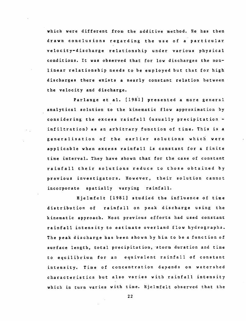
Parlange et al. (1981] presented a more general

analytical solution to the kinematic flow approximation by

considering the excess rainfall (usually precipitation -

infiltration) as an arbitrary function of time. This is a

generalisation of the earlier solutions which were

applicable when excess rainfall is constant for a finite

time interval. They have shown that for the case of constant

rainfall their solutions reduce to those obtained by

previous investigators. However, their solution cannot

incorporate spatially varying rainfall,

Hjelmfelt (1981] studied the influence of time

distribution of rainfall on peak discharge using the

kinematic approach, Most previous efforts had used constant

rainfall intensity to estimate overland flow hydrographs.

The peak discharge has been shown by him to be a function of

surface length, total precipitation, ·storm duration and time

to equilibrium for an equivalent rainfall of constant

intensity. Time of concentration depends on watershed

characteristics but also varies with rainfall intensity

which in turn varies with time, Hjelmfelt observed that the

22

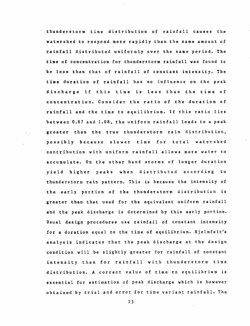
thunderstorm time distribution of rainfall causes the

watershed to respond more rapidly than the same amount of

rainfall distributed uniformly over the same period. The

time of concentration for thunderstorm rainfall was found to

be less than that of rainfall of constant intensity. The

time duration of rainfall has no influence on the peak

discharge if this time is less than the time of

concentration. Consider the ratio of the duration of

rainfall and the time to equilibrium. If this ratio lies

between 0.87 and 1.08, the uniform rainfall leads to a peak

greater than the true thunderstorm rain distribution,

possibly because slower time for total watershed

contribution with uniform rainfall allows more water to

accumulate. On the other hand storms of longer duration

yield higher peaks when distributed according to

thunderstorm rain pattern. This is because the intensity of

the early portion of the thunderstorm distribution is

greater than that used for the equivalent uniform rainfall

and the peak discharge is determined by this early portion.

Usual design procedures use rainfall of constant intensity

for a duration equal to the time of equilibrium. Hjelmfelt's

analysis indicates that the peak discharge at the design

condition will be slightly greater for rainfall of constant

intensity than for rainfall with thunderstorm time

distribution. A correct value of time to equilibrium is

essential for estimation of peak discharge which is however

obtained by trial and error for time variant rainfall. The

23

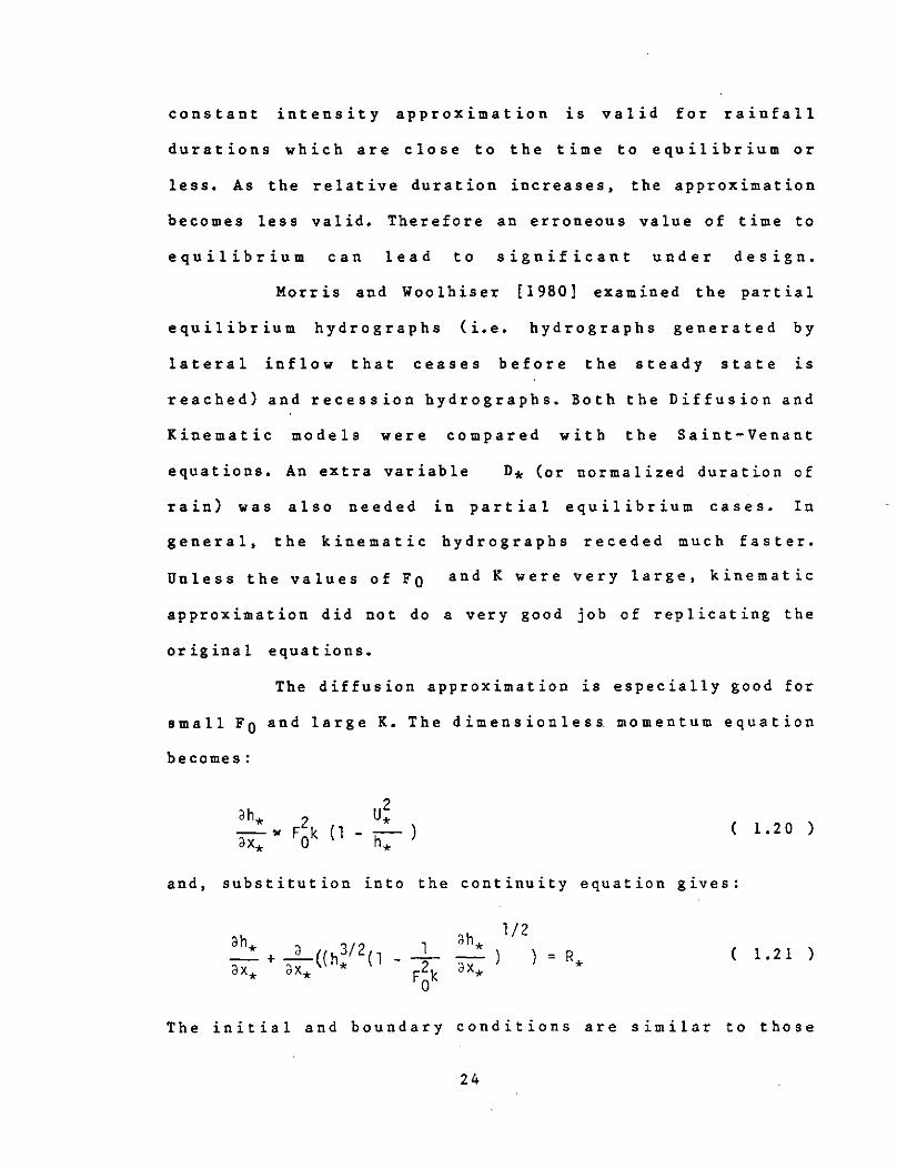
constant intensity approximation is valid for rainfall

durations which are close to the time to equilibrium or

less. As the relative duration increases, the approximation

becomes less valid. Therefore an erroneous value of time to

equilibrium can lead to significant under design.

Morris and Woolhiser [1980] examined the partial

equilibrium hydrographs (i.e. hydrographs generated by

lateral inflow that ceases before the steady state is

reached) and recession hydrographs. Both the Diffusion and

Kinematic models were compared with the Saint-Venant

equations. An extra variable D* (or normalized duration of

rain) was also needed in partial equilibrium cases. In

general, the kinematic hydrographs receded much faster.

Unless the values of Fo and K were very large, kinematic

approximation did not do a very good job of replicating the

original equations.

The diffusion approximation is especially good for

small Fo and large K. The dimensionless. momentum equation

becomes:

( 1.2 0 )

and, substitution into the continuity equation gives:

ah* + _a_((h!/2( 1 3h*

1/2 1 ( 1.21 )

F2

k ) ) = R*

ax* ax* ax* 0

The initial and boundary conditions are similar to those

24

discussed by Vieira [1983] and appear later in the text(see

page 25). Morris and Woolhiser [1980] used an implicit

finite difference scheme to solve equation (1.21) and have

compared the results with the Saint-Venant equations. The

diffusion wave does a very good job of replicating the

rising limbs of the partial equilibrium hydrographs. As Fo

tends to zero and K tends to infinite the diffusion equation

approaches the full Saint-Venant equations. Morris and

Woolhiser concluded that the complete Saint Venant equations

or at least the diffusion equation must be used for overland

flows on flat grassy slopes, even though K may be very

large.

In his paper (referred to earlier in the this

chapter) Vieira [1983] examines the validity of

approximations for the Saint-Venant equations for overland

flow, He started by considering the solution through

characteristic curves and stated that, for subcritical

flows, the solution domain may be divided into four zones

viz. A,B,C,D, see e.g. Woolhiser and Liggett [1967], He has

then further analyzed the nature of the solution in each

zone, The dimensionless equations (1.15) and (1.16) are re-

written here for convenience in the notation used by Vieira:

.£!! + u .£!! + ~= 1 aT ax ax

( l.22a )

2.1!. + u 2.!!.. + F-2(aH) k ( 1 -u2 lJ

= -) - H aT ax o ax H ( l.22b )

( where all symbols have usual significance ) ,

25

In Zone A, the solutions are dependent only on the

initial condition of the dry channel. Bence equations

(l.22a) and (l.22b) reduce to ordinary differential

equations. The differential equations have been solved

analytically using the initial conditions (1.23) by

Brutsaert [1968]:

U(X,0) = B(X,0) = 0 ( 1.23 )

For large K it was found that the solution is of the form

B = T , U = Tl/2 ( 1.24 )

As T increases, the upper and lower boundary conditions

begin to take effect. TaS (see equation (1.19)) is the value

where the Zone A solution ceases. In case of supercritical

flows Zone A is bounded by line T = 0, X =land the forward

characteristic starting at the point X = O, T = O. The flow

is influenced only by initial and upper boundary conditions.

In Zones B, C and D, Woolhiser and Liggett [1967]

used characteristics method for solving the equations for

subcritical flow using the following boundary conditions.

U(O,T) = 0 ( 1.25 )

U(l,T) = B(l,T)l/2/Fo ( 1.26 )

When the characteristics method was not suitable, they used

an implicit finite difference scheme which is generally

suitable for medium sized computers. However solutions for

Fo < 0,4 and for large values of K could not be obtained

26

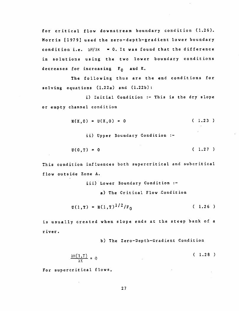
for critical flow downstream boundary condition (1.26).

Morris [1979] used the zero-depth-gradient lower boundary

condition i.e. aH/ax = O. It was found that the difference

in solutions using the two lower boundary conditions

decreases for increasing F 0 and K.

The following thus are the end conditions for

solving equations (l.22a) and (l.22b):

i) Initial Condition :- This is the dry slope

or empty channel condition

H(X,0) = U(X,0) = 0 ( 1.23 )

ii) Upper Boundary Condition·-

U(O,T) = 0 ( 1.27 )

This condition influences both supercritical and subcritical

flow outside Zone A.

iii) Lower Boundary Condition:-

a) The Critical Flow Condition

U(l,T) = H(l,T) 1 f 2 /Fo ( 1.26 )

is usually created when slope ends at the steep bank of a

river.

b) The Zero-Depth-Gradient Condition

aH(l ,T) = O ax

For supercritical flows,

( 1.28 )

27

U(l,T) > H(l,T)l/2/Fo ( 1.29 )

The kinematic wave approximation is valid for K >

50, and all the other terms in the momentum equation (1.19)

are negligible when compared to the term k(l - u2;H).

Equation (l.22b) reduces to

k( l-U 2 H) = 0 ( 1.30 )

Hence,

u2 = H ( 1.31 )

which, on substitution into equation (l.22b) yields the

Kinematic Wave Equation:

l!:!_ + a(H3/2) aT ax = 1 ( 1. 3 2 )

Equation (1.32) may be solved using the initial condition

(l.23) to obtain the solution given by equation (l.24). The

rising portion of the hydrograph is given by

Q=HU=T3/2 (1. 3 3)

There is only one hydrograph for this approximation as the

equation (1.32) is independent of Fo and K. The hydrograph

rises as T 3 / 2 till equilibrium when T = 1, then Q = 1 for

all values ofT>l.

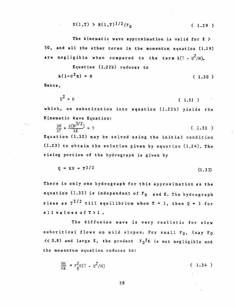
The diffusion wave is very realistic for slow

subcritical flows on mild slopes, For small Fo, (say Fo

<< 0.8) and large K, the product Fo2K is not negligible and

the momentum equation reduces to:

( 1.34 )

28

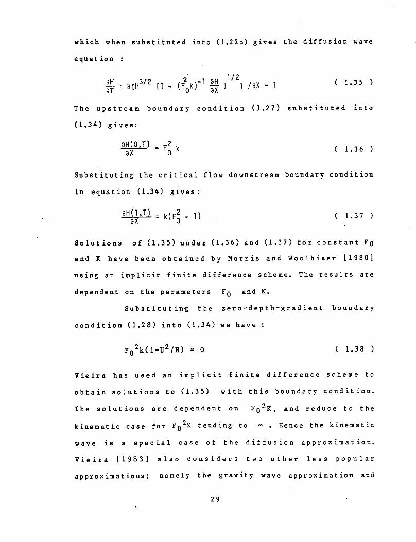
which when substituted into (l.22b) gives the diffusion wave

equation

( 1.35 )

The upstream boundary condition (1.27) substituted into

(1.34) gives:

aH(O,T) = ax F

2 k

0 ( 1.3 6 )

Substituting the critical flow downstream boundary condition

in equation (1.34) gives:

aH(l,T) = k(F20

_ l) ax ( 1.37 )

Solutions of (1.35) under (1.36) and (1.37) for constant Fa

and K have been obtained by Morris and Woolhiser [1980]

using an implicit finite difference scheme. The results are

dependent on the parameters F 0 and K.

Substituting the zero-depth-gradient boundary

condition (1.28) into (1.34) we have :

( 1.38 )

Vieira has used an implicit finite difference scheme to

obtain solutions to (1.35) with this boundary condition.

The solutions are dependent on F 0 2K, and reduce to the

kinematic case for F 02K tending to ~ . Hence the kinematic

wave is a special case of the diffusion approximation.

Vieira [1983] also considers two other less popular

approximations; namely the gravity wave approximation and

29

the zero depth gradient approximation.

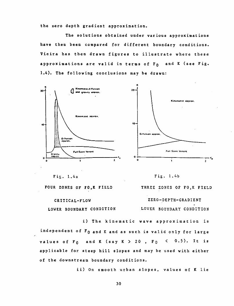
The solutions obtained under various approximations

have then been compared for different boundary conditions.

Vieira has then drawn figures to illustrate where these

approximations are valid in terms of Fo and K (see Fig.

1.4). The following conclusions may be drawn:

• 20

,a

I'\ K.,.."'•loe:.d,llus,o" ~ and 9ra.o1, •rtOro•.

OJ_.,!!!~'--..:::,,_ _________ ,,

0 '

Fi:;. l.4a

FOUR ZONES OF FO,K FIELD

CRITICAL-FLOW

LOWER BOUNDARY CONDITION

• 20

Kin,em,111c app,o•.

10

Fig. l.4b

THREE ZONES OF FO,K FIELD

ZERO-DEPTH-GRADIENT

LOWER BOUNDARY CONDITION

i) The kinematic wave approximation is

independent of Fo and K and as such is valid only for large

values of Fo and K (say K > 20 Fo < 0.5). It is

applicable for steep hill slopes and may be used with either

of the downstream boundary conditions.

ii) On smooth urban slopes, values of K lie

30

between 5 and 20; both kinematic and diffusion

approximations are valid and either of them may be adopted.

However for lower values of F 0 , (say F 0 < 0.5) the diffusion

wave is very good. It performs better than the kinematic

wave for all cases.

iii) The zero-depth gradient condition should

be used for higher values of Fo and K. The Diffusion Wave

results are sensitive to F 0 2K. It is interesting to note

that the hydrographs are dependant on the product Fo 2K, and

not on F 0 and K individually.

The study presented by Vieira has clearly stated

the conditions under which any particular approximation may

be valid - very useful information for the practising

engineer. For reasons already mentioned, the full Saint­

Venant equations are rarely used.

1.4 PROJECT OBJECTIVES :-

The overall objective of this report is to

determine new analytical solutions to the hydraulics of the

overland flow problem to provide depth and discharge values

over the flow domain under physically justifiable initial

and upstream-downstream boundary conditions, This is

achieved through the following:

a) The hydraulic equations of gradually varied

unsteady overland flow (Saint Venant Equations) are

approximated by the diffusion wave which is more realistic

than the kinematic wave. The diffusion wave model is

developed for the overland flow plane and many cases of

31

initial and end conditions of practical interest are

considered.

b) The approximate analytical solutions for the

diffusion wave model of overland flow are developed and then

tested by

i) the comparison of these solutions with the

corresponding numerical solutions of the diffusion wave and

the full Saint Venant equations under various hydraulic,

topographic, boundary and rainfall-infiltration conditions

which are typical of Eastern Kentucky watersheds. The

numerical kinematic wave solutions are also obtained to

compare the performance of the diffusion wave against the

kinematic wave.

ii) the comparison of these approximate

analytical solutions of the diffusion wave to those

numerical results of overland flow studies given in the

literature.

32

CHAPTER 1. SOLUTION FOR STEEP SLOPES

2.1 DESCRIPTION ·-

As discussed in the previous chapter, analytical

solutions to the full Saint-Venant equations are very

difficult to obtain if not impossible. The diffusion wave

approximation itself is not amenable to complete analytical

solution without some further simplifications. It has been

stated in the literature (e.g. Morris [1978]. Vieira [1982))

that under the cases of large F 0 and K, the zero-depth­

gradient downstream boundary condition is a justifiable

substitute to the critical depth condition, The upstream

boundary condition is one of zero influx. This· implies that

while there is no inflow at x = 0, it is possible to have a

finite depth with time. This condition does not match with

the initial condition of zero depth (i.e. the dry channel

condition) and hence causes some uncertainty at the point x

= 0 and t = O. This difficulty may be avoided while using

finite difference schemes by using backward differencing for

the first few time steps and then switching to a more

accurate Crank - Nicolson type scheme. In this way no

decision needs to be made about values at the

initial/boundary points at the corners.

33

However when steep slopes are being considered,

there is not much scope for the water to accumulate at the

top of the overland flow plane (x = 0) as it will flow away

immediately. Hence the water depth here is practically

negligible for all times t > O. Under these circumstances

it is reasonable to assume

h(O,t) = 0 ( 2 .1 )

as the upstream boundary condition. This assumption is

further strengthened when performing the steady state

analysis for the diffusion wave. This chapter deals with a

numerical series solution for the diffusion wave under the

upstream boundary condition of (2.1) and zero-depth-gradient

downstream boundary condition. The first two and three terms

in the series are considered to demonstrate the efficacy of

this method as compared to finite differencing or the method

of characteristics. Semi analytical solutions are also

obtained under the above mentioned conditions. These

analytical solutions are compared to the complete Saint

Venant equations (see Fig. 2.2,2.3).

2.2 THEORY OF THE NUMERICAL SERIES SOLUTION:-

The governing differential equation is

ah 1;2 E ~) } = q(x,t) ax

( 2.2 )

where,

( 2. 3 )

subject to an initial condition of

34

h(x,O) = 0

and the boundary conditions

h(O,t) • 0

ah(l,t) = O ax

( 2.3a )

( 2.4a )

( 2.4b )

Assume that the solution is of the form given by the

following infinite sine series ,

ii = i: ( 2. 5 ) n=l

where hn(t), n = 1,2, ••• , , are all functions of time only

and the x dependence comes from the sine terms. It may be

further assumed that the first few terms of the series are

the dominant ones and the contribution of terms for higher n

is negligible. In fact, it was found that for most

instances, two or three terms are quite adequate. Hence

where h

N -h = i:

n=l h (t)

n sin ( 2. 6 )

is an approximation to hand is equal to h for

sufficiently large N.

A variant of Galerkin's method is now adopted. The

interval of interest (0,1] is partitioned into N equal

subintervals. The residual ~ is defined as

ah = -+

at 3 {h3/2 (1 - E 3x

ah 1/2 -) } ax - q(x,t) ( 2. 7 )

From (2.6) we notice that there are N unknowns

(i.e. n = 1,2, .... ,N) and hence N independent

differential equations are required. These are obtained by

35

integrating the residual over each of the N subintervals and

setting it to zero. The partition of the interval is given

by

O l 2 N-1 ~:O = - < - < - < •••• < -- <

N N N N N = 1 N

and the N differential equations are obtained from

K/N JK-1 ~ dx = 0

N

, k = 1,2,•••,N

ah ax at

K/N a + 1K-l ax

N

3/2 {h (1 - E

ai, 112 ) }dx -

ax

K/N

f K-1

N

q(x,t)dx

k = 1,2, ••• ,N

( 2. 8 )

0

( 2 • 9 )

The equation (2.9) may be stated in matrix form as

[R]{h} + {F} - {Q} = {O} ( 2.10)

where the following results are obtained after

simplification

[R] = r -kn -

{ F} =

and • {Q}

and {h}

2 [cos { (2n-l) ,r (k-1)} (2n-l),r 2 N

- cos { (2n-l) n k} 2 N

for n,k = 1,2, ....... ,N ( 2.11 )

3/2 :ii, I K/N

fk = h (1 - E -) ax K-1

N

k = 1,2, ..... , N ( 2 .12

= qk = !KIN q(x,t)dx K-l_

N

k = 1,2, ..... , N ( 2 .13

is the vector denoting the derivatives of

36

)

)

the components hn (n = 1,2, ... ,N) with respect to time.

This then provides a system of ordinary

differential equations. Note that the form of the solution

chosen in equation (2.5) automatically satisfies the

boundary conditions stated above. The initial condition is

satisfied when solving the N initial value problems obtained

from (2.10) under the following starting conditions

n = 1,2, •••••• ,N ( 2.14 )

The system of ordinary differential equations

given by (2.10) has been solved numerically by using the

IMSL subroutine DVERK which employs a Runge-Kutta-Verner

fifth and sixth order method. It has automatic error and

step size control capabilities and was found to be reliable

for this problem. For a large N, the matrix R has been

inverted using another IMSL routine LINV2F which produces

high accuracy solutions. The. performance of this numerical

technique has been shown in Fig. 2.2.

2.3 THEORY OF THE ANALYTICAL SOLUTION:-

The numerical solution discussed in the previous

chapter provides sufficient insight to obtain analytical (or

semi-analytical) solutions. These are dependent on the

number of terms chosen in the series solution. The theory

involved in using two terms is explained in this section and

may be easily generalised to include cases for larger N.

components

It may be assumed that h(x,t), and hence all the

hn(t), approach a constant asymptotic value for

37

• a • • A L I z E a a I s c • A • G E

• a • • A L I z E a a I s c

" A • G f

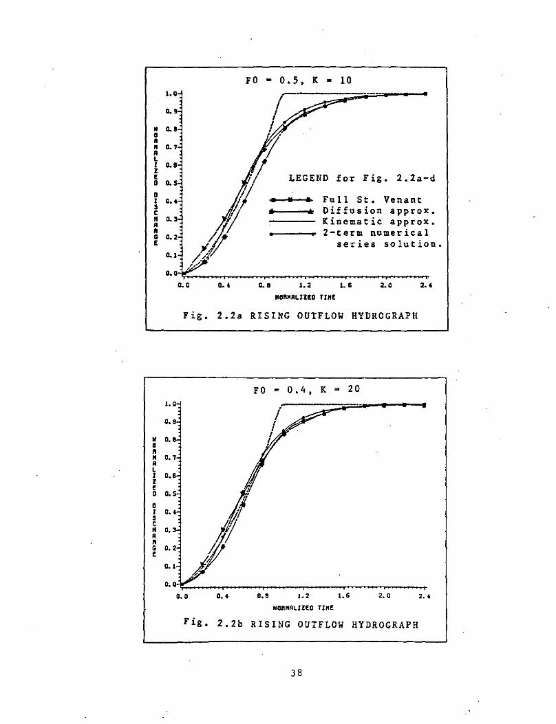
FO • 0.5, K • 10 1.0

0.9

0.1

0.1

a.a

0.

o ••

0.3

0.2

0.1

a.a a. a a.• o ••

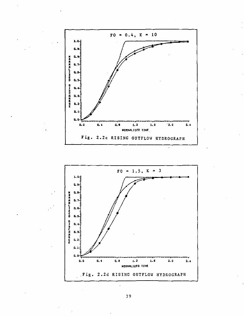
LEGEND for Fig. 2.2a-d

• • • Full St. Venant Diffusion approx. Kinematic approx. 2-term numerical

series solution.

1. 2 1. 6 2.0

NGIIMALIZ!O TJM!

Fig. 2.2a RISING OUTFLOW HYDROGRAPH

FO = 0. 4, K = 20 1. a-1

a.a

0. 8

a.,

a.s

a.s

1 a.• /!; 'I, r a. 3

a. 2 !J a. I ~ a. a

a. a a.• a.a ,. 2 1.6 2. a 2 ••

NC,,"ALJZEO TJ"I!:

Fig. 2.2b RISING OUTFLOW HYDROGRAPH

38

I. Q

a.

N 0. a • • A l I D. z ! Q a. D I • c " a. A • C 0.2 !

0.1

I. Q

a. 9

N a. a

" " A l I o. l E D a. s D I o ••

' c

" o •• A

" G 0.2 E

O. I

o. 0

FO = 0.4, K = 10

a. o Q •• D. a 1. 2 I. a ·2. Q

NOft.~ll!!C TJH!_

Fig. 2.2c RISING OUTFLOW HYDROGRAPH

FO = 1. 5. K = 3

-I I r

1 II I '

!/ ; '

/f/ ,,

~_,.· ~

o. 0 a.• o. a ,. 2 1. 8 2. 0

M!Jlll'IALJ Z!D TIS!

. Fig. 2.2d RISING OUTFLOW HYDROGRAPH

39

2..

2 ••

• 0. a ft • A l I o. z E Q 0.

0 I Q. s c • o. A ft ~ E

o ••

0.J

o. 0

J.

o.

• 0. a ft • 0.1 A L I o. s z E Q o. Q I Q ••

• c H o •• A

" c 0.2 E

Q. 1

0. Q

JI ., u.o Q ••

FO = 0.4, K = 20

0 ••

LEGEND for Fig. 2.2e-j

1 • Full ·St. Venant ' .._ Diffusion approx.

Kinematic approx. --~-- 3-term numerical

series solution.

J. 2 J.8 2.0

NCft)fAl!l!D JJ)I,

Fig. 2.2e RISING OUTFLOW HYDROGRAPH

FO = o.s, K = 10

o. Q O.t a. a J. 2 1. 8 z. a z •• NOl'\:,t.:ILJI!D Tl:tl!

Fig. 2.2f RISING OUTFLOW HYDROGRAPH

40

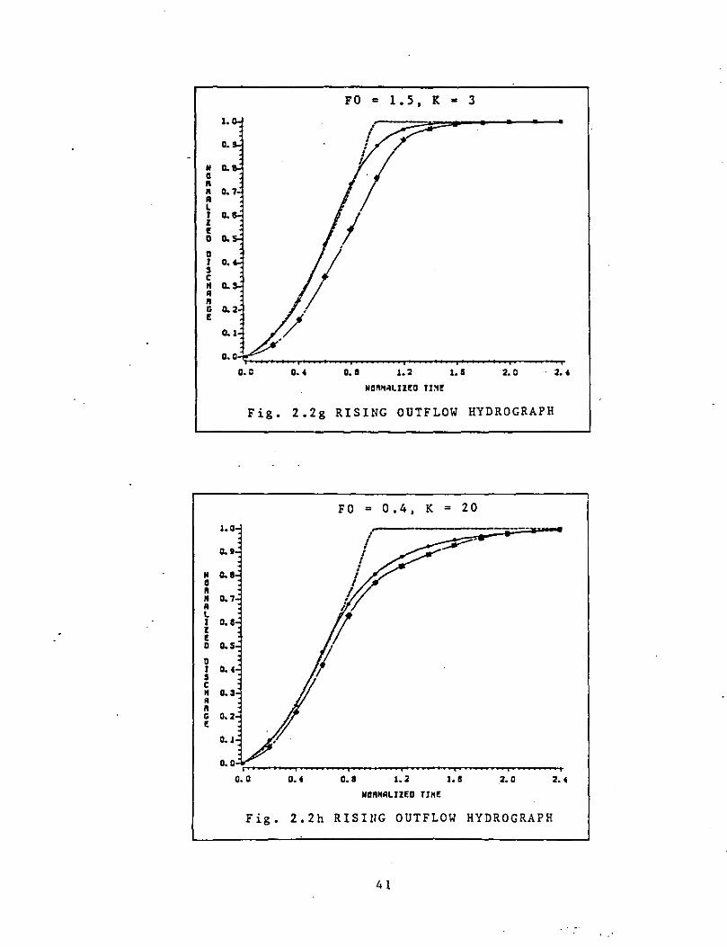
FO = 1. 5. K • 3

I.

a.

• 0. • ft • A L I a. • ! D a. D I o.

' c • a. A ft G a.2 !

0.1

a.a a. a o •• o. a 1. 2 1. 5 2. 0 2 ••

Nl:ll'l!'lilllZ!D Tia!

Fig. 2.2g RISING OUTFLOW HYDRO GRAPH

FO = 0 • 4, K = 20 1. 0

a.1 -;,--·

• a.a • ft • a. 7 A L I o. 5 z ! D a.s D I 0..

' c • a.,

" • G o. 2 !

0.1

o. a a. a a., a. a I. 2 I. I 2. a 2 ••

NGANALIZED TIN!

Fig. 2.2h RISI!IG OUTFLOW HYDROGRAPH

41

H • • • o. 7 • l 1 o. a l ! 0 0.

0 1 • c N 0. •

FO = 1.5, K = 10

• c ! c. 21

o. 1

"'.....:;;;·~---....... o.o ..-~..-~ .... ~--.~~..-~ .... ~-.~~ .... ~ ..... ~ ..... ~-...

• • • • • l I l ! D

0 I • c • • • G !

1.

a.

0.

o.

o ••

o.,

o. 2

0.1

o.o 0.2 o., o.a o.a 1.0 1.2 1., 1.a 1.a. 2.0 NGIINRLJZ!D TJMf

Fig. 2.2i RECESSION OUTFLOW HYDROGRAPH

FO = l . 5 , K = 3

-..::.._ .. -.... o. 0-

c.o o. 2 a.. 0. s o. a J. D 1. 2 1 •• 1. S 1. a 2. a NCi,KRLlZEO. TJJ'I!!:

Fig'. 2. 2 j RECESSION OUTFLOW HYDROGRAPH

42

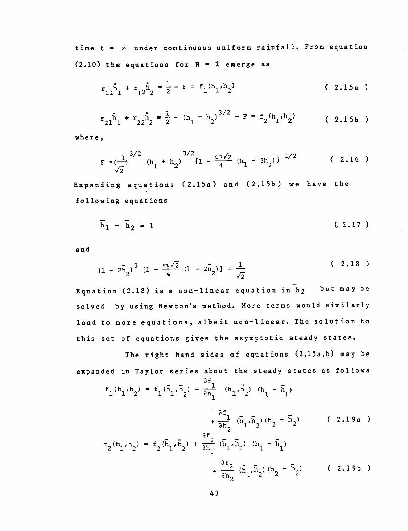
time t = "" under continuous uniform rainfall. From equation

(2.10) the equations for N = 2 emerge as

l = - - F =

2

h + r h = !. - (h - h )3

/2

+ F = r21 l 22 2 2 l 2

where,

l 3/2 F =(-)

r'2

( 2.15a )

( 2.15b )

( 2.16 )

Expanding equations ( 2.15a) and ( 2.1 Sb) we have the

following equations

(2.17)

and

( l 2h ) 3 [ l - ET, r'2 (1 - 2h ) ] = ..!.._ +2 4 2 fi

( 2.18 )

Equation (2.18) is a non-linear equation in hz but may be

solved by using Newton's method. More terms would similarly

lead to more equations, albeit non-linear. The solution to

this set of equations gives the asymptotic steady states.

The right hand sides of equations (2.15a,b) may be

expanded in Taylor series about the steady states as follows

afl fl (h1,h2l = f1 <ii1,ii2l + ah1 Ch1,h2l <h1 - h1>

( 2.19a )

( 2.19b)

43

From (2,15a,b), we have

fl (hl,h2) = f2(hl,h2) = O

Equations (2.19a,b) may be written as

f2 (hl,h2) = a21 h + a h + b 1 22 2 2

where,

[A] = [ a .. l ati ci\,ii2 l

= 1J ahj

{K} = =

( 2.20 )

( 2.2la)

( 2.2lb )

i,j = · 1, 2 ( 2.22a )

....... ( 2.22b )

Say [BJ = [R]- 1 [A] and {D} = [R]- 1 {K}. Substituting these

relations in ( 2.21 ) we have

{h} = [ B ] • ( h} + { D} ( 2.23 )

where {h} ~ {hk}, is the vector of solution components to

be substituted in (2.6).

This is a linear system of differential equations

with constant coefficients. Its solution may be expressed as

follows

[BJ (t-t0

) {h(t)} = e {c} + ( 2.24 )

where the column vector (C} is obtained from the initial

condition at time t = t 0 • Therefore

{h(t 0 l} = {C} ( 2.25 )

44

2,3,1 The Rising Hydrograph :-

F o r t h e r i s in g p o r t i o n o f t he h y d r o gr a p h, t O = 0

and {c} = {O}. Hence the solution reduces to the form

t {h ( t)} = f e [BJ ( t- s) {D} d s ( 2 .2 6 )

0

This expression has been evaluated by using

eigenvalue theory (see Bronson [1973], chp, 29) to obtain

the rising portion of the hydrographs.

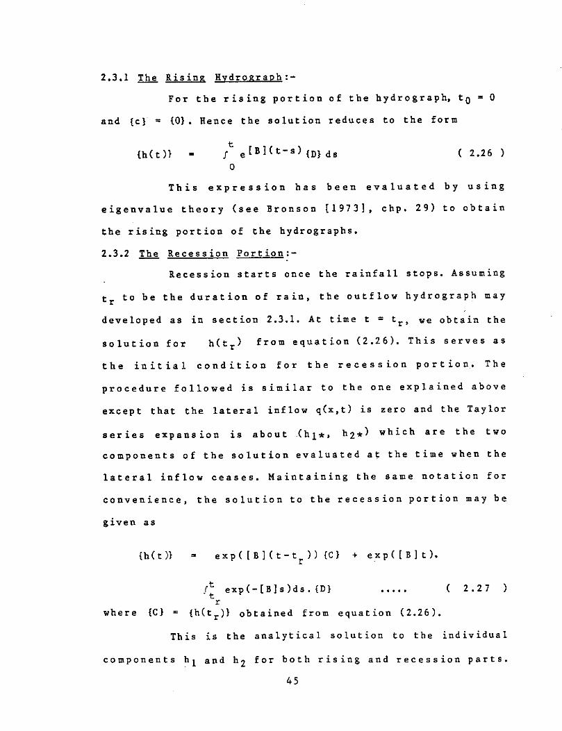
2.3.2 The Recession Portion:-

Recession starts once the rainfall stops. Assuming

tr to be the duration of rain, the outflow hydrograph may

developed as in section 2.3.1. At time t = tr, we obtain the

solution for b(tr) from equation (2,26), This serves as

the initial condition for the recession portion, The

procedure followed is similar to the one explained above

except that the lateral inflow q(x,t) is zero and the Taylor

series expansion is about .(bl*• h2*) which are the two

components of the solution evaluated at the time when the

lateral inflow ceases, Maintaining the same notation for

convenience, the solution to the recession portion may be

given as

{h ( t )}

where {C} =

= exp([B](t-tr)){C} + e.xp([B]t),

!~ exp(-[B]s)ds, {D} r

{h(tr)l obtained from equation (2.26).

( 2.27 )

This is the analytical solution to the individual

components h 1 and b 2 for both rising and recession parts.

45

• a • • • L 0. I • ' D

D I

' r • • • • !

• a • • • l I l

' a D I

' r • • • • '

1.

a.

0.

Q,

0.

Q,

a. a o.,

FO • 0.5, K = 10

0.1

LEGEND for Fig. 2.3a-e

1.2

Full St. Venant Diffusion approx, Kinematic approx. 2-term analytical

series solution •

l. I 2.0 2 ••

ND~MRLIUD TIM!

Fig. 2.Ja RISING OUTFLOW HYDROGRAPH

FO = 0.707, K = 3

i I I I I

I

a. a a.• 0. I l. 2 I. I 2. Q 2 ••

IIIIS,.NALJ?!D TIM!

Fig, 2,Jb RISIRG OUTFLOW HYDROGRAPH

46

FO = 1. 0. K = 20 a. a

0.1

0.1

• a a., • • A 0.1 L

I z 0.5 !

D

D a.. I

' a., c • • 0.2 • ' ! 0.1

a.a a.a a., 0.1 I. 2 t. I :z. a 2 ••

NBRNALIZ!D TIN!

Fig. 2.3c RISING OUTFLOW HYDROGRAPH

FO = 1. 0, K = 3 I. 0

0.1

• a. a • 0.7 • A L 0.1 I z ! o. 5 D

D a.. I

' c o. 3 • • • o. 2

' ! 0.1

o. 0

O. D D. t D. I ,. 2 J. a 2. 0 2.'

Fig. 2.3d RISING OUTFLOW HYDROGRAPH

47

FO = 0,707, K = 3 1.a

a.1

a., • a a.1 " • • G. I l

' z a. s ! D

D a.. I • a., c • • a.2 " ; !• a.1

a.a a. a a. 2 a.• 0..1 0..9 1.0 1.2 1.6 I.& I.I Z.0

tU:lft,'lijlJZ!D TJ;it!

Fig, 2,Je RECESSION OUTFLOW HYDROGRAPH

FO = l • 0, K = 3 t.

LEGEND for Fig. 2.3f • a. • • Full St. Venant " a. 1 • Kinematic • approx • l a.1 2-term analytical I z s er ie s solution. ! a. s a a a.. ' • c a., • • • a. 2 ; t

a. I

a. a. a a. 2 a., 0.1 a.a 1. a 1.2 I. t I. I ,. a 2. a

NC,.i1RLJZ!D TJi1!

Fig, 2.3f RECESSION OUTFLOW HYDROGRAPH

48

The complete solution with space dependence may be obtained

by substituting in equation (2.6). Fig. 2.3 shows the

performance of this technique,

2.4 PERFORMANCE OF THE SERIES SOLUTION SCHEME ·-

The numerical solution discussed in section 2.2

has many advantages in comparison to the method of

characteristics and finite differencing. It is

computationally more efficient and simpler to formulate. It

does not use any variant of Newton's method for solving a

set of non-linear equations as in the method of

characteristics or finite differencing and hence saves a lot

of time. It involves solving a system of initial value

problems for which good software packages are available. The

IMSL subroutine DVERK is found to be adequate for this

problem, The program performs eight function evaluations per

step and from these two estimates of the dependent variable

are obtained based on the fifth and sixth order

approximations. A comparison of these two estimates provides

a basis for step size selection. The equations appearing in

the analysis are simple in form and structure. The level of

accuracy may be increased by increasing the number of terms

considered in the sine series.

The major setback of the analytical solution seems

to be the solution of a system of non linear equations to

obtain the steady state values for each case of F 0 , Kand

rainfall intensity. This can be avoided by using TABLE 2.1

which presents the steady state values for two term sine

49

series solutions under a constant and uniform dimensionless

l,a t er a 1 inf 1 ow of 1. 0. Inter med i ate values may be obtained

through a similar procedure (Section 2.3).

The numerical series solution for the case of N =

2 performs better than both the method of characteristics

and finite differencing. The solution obtained on

considering three terms in the series is better than the two

term approximation and is practically coincident to the

solution obtained from the numerical solution to the Saint

Venant equations. This means that convergence i-s very fast

and very few terms are required for most practical cases.

This is perhaps the most desirable feature of this new

method.

This technique also provides valuable insight into

the problem and provides guidelines for developing an

analytical solution for both rising and recession portions.

The two term analytical solution overestimates the outflow

hydrographs in the initial region. However as time increases

and the steady state is approached, the solution becomes

very good. This is expected since, for the rising portion of

the hydrograph, the right hand sides of equations (2.15a,b)

are expanded in Taylor series about the steady state. The

truncated series is therefore a good approximation in the

neighbourhood of the steady state but looses accuracy as it

moves further away in time. The overall shape of the profile

is similar to the numerical Saint Venant solution. The

recession portion has typical exponential behaviour and is

50

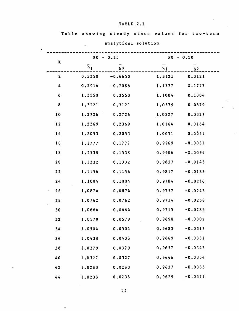
TABLE 2.1

Table showing steady state values for two-term

analytical solution

------------------------------------------------------------FO = 0.25 FO = 0.50

K

hi h2 bl h2 ------------------------------------------------------------2 0,3350 -0.6650 l. 3121 0.3121

4 0.2914 -0.7086 1.1777 0.1777

6 1.3550 0.3550 l. l 004 0.1004

8 1.3121 o.3121 1.0579 0.0579

10 1.2726 0.2726 l,0327 0.0327

12 1.2369 0.2369 1.0164 0.0164

14 1.2053 0.2053 1.0051 0.0051

16 1.1777 0.1777 0.9969 -0.0031

18 1.1538 0.1538 0.9906 -0.0094

20 1.1332 0.1332 0.9857 -0.0143

22 1.1156 0.1156 0.9817 -0.0183

24 1.1004 0.1004 0.9784 -0,0216

26 1.0874 0.0874 0.9757 -0,0243

28 1.0762 0.0762 0.9734 -0.0266

30 1,0664 0.0664 0.9715 -0,0285

32 1.0579 0.0579 0.9698 -0.0302

34 1. 0 5 04 0.0504 0,9683 -0.0317

36 1.0438 0.0438 0.9669 -0.0331

38 1.0379 0.0379 0.9657 -0.0343

40 1.0327 0.0327 0.9646 -0.0354

42 1.0280 0.0280 0.9637 -0.0363

44 1.0238 0.0238 0.9629 -0.0371

5 1

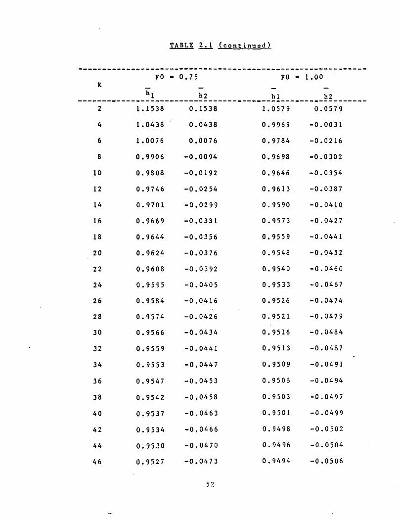
TABLE .hl (continued)

------------------------------------------------------------FO a 0.75 FO = 1.00

IC

hi h2 hl h2 ------------------------------------------------------------2 1.1538 0.1538 1.0579 0.0579

4 1.0438 0.0438 0.9969 -0.0031

6 1,0076 0.0076 0.9784 -0.0216

8 0.9906 -0.0094 0. 96 98 -0.0302

10 0.9808 -0.0192 0.9646 -0.0354

12 0.9746 -0.0254 0.9613 -0.0387

14 0.9701 -0.0299 0. 9 5 90 -0.0410

16 0.9669 -0.0331 0.9573 -0.0427

18 0.9644 -0.0356 0.9559 -0.0441

20 0.9624 -0.0376 0.9548 -0.0452

22 0.9608 -0,0392 0,9540 -0.0460

24 0.9595 -0.0405 0,9533 -0.0467

26 0.9584 -0.0416 0,9526 -0.0474

28 0.9574 -0.0426 0.9521 -0.0479

30 0.9566 -0,0434 0.9516 -0.0484

32 0.9559 -0.0441 0.9513 -0.0487

34 0.9553 -0,0447 0.9509 -0.0491

36 0.9547 -0.0453 0.9506 -0.0494

38 0.9542 -0.0458 0.9503 -0.0497

40 0.9537 -0.0463 0.9501 -0.0499

42 0.9534 -0.0466 0.9498 -0.0502

44 0.9530 -0.0470 0.9496 -0.0504

46 0.9527 -0.0473 0.9494 -0.0506

52

reasonably close to the corresponding numerical results.

53

CHAPTER .b_ ANALYSIS OF STEADY STATE

3.1 DESCRIPTION :-

One of the ways of tackling highly non linear time

and space dependent partial differential equations is to

assume the solution to be composed of two parts, The first

part consists of solving the problem assuming steady state

conditions exist. This is physically justifiable for the

problem under consideration since if the rain durat.ion is

infinite (practically speaking tr greater than time of

concentration of the reach) a steady state is achieved. The

problem reduces to an ordinary non linear differential

equation for the one dimensional overland flow, The second

part of the solution process involves finding transient

solutions which when superimposed on the steady state

solution, yield the complete solution.

The steady state solution also provides a better

understanding of the nature of the water profile. It may,

for example, provide information on the cases when zero

depth upstream boundary condition may be used instead of the

zero influx condition. This important aspect of the solution

of the process has received very little attention in the

literature, An efficient method for numerically evaluating

the steady state profiles and analytical approximations for

54

some of the cases are developed in the following sections.

3.2 THE STEADY STATE THEORY :-

The steady state diffusion equation is given by

~ {h 3/2(l _ E dh dx dx

-q (x)

where, h(x) is the steady state solution,

lirn q(x,t) = q(x) t--

lirn h(x, t) = h(x) t--

( 3 .1 )

( 3.2a )

( 3.2b )

The steady state solution h(x) is such that it satisfies

the boundary conditions for the complete solution h(x,t).

Therefore the initial condition is satisfied by the

transient solution. Hence

dh (0) = a ( 3 .3a )

dx

dh (1) = b

( 3.3b )

dx

where a and b = for critical depth

downstream boundary condition and b = 0 when zero-depth-

gradient downstream boundary condition is used.

Equations (3.1) and (3.3) constitute a non linear

two point boundary value problem which is rather difficult

to solve. Integrating equation (3.1) over the interval

[O,l], we obtain

- 3/2 dh (1) 112

h(l) (1 - E dx ) h(O) 312

(1 - E

- 1/2 dh(O)) = fol q (x)dx (

dx 3. 4 )

Substituting the boundary values from (3.3), we have

55

which reduces after simplification to

h(l) = {(l - Eb)-112 f~ q(x)dx}213

r1 q(x)dx 0

( 3. 5 )

( 3. 6 )

This provides an analytical expression for the steady state

ordinate at x = 1. For constant and uniform rain q(x) = 1,

and

h (1) = (1 - Eb) -l/3 ( 3. 7 )

For er it ical depth lower boundary condition, we have from

equation (3. 7)

h(l) = Fo2/3 ( 3. 8 )

and the corresponding expression for the zero-depth-gradient

downstream condition is

h(l) = 1 ( 3. 9 )

It may also be noticed that for F 0 = 1 • bis

identically zero for all values of K. Under this condition

the steady state profile for either lower boundary condition

is the same.

3.3 .I!!l NUMERICAL STEADY STATE SOLUTION:-

Integrating equation (3.1) over [O,x] we have

- 3/2 dh 1/2 x - ( 3 1 O ) h(x) (1 - Edx) = !

0 q(x)dx •

Under conditions of constant rainfall, equation (3.10) is

56

b.3(1 - e::) = x2

Using the transform at ion x + z = 1, we have

dh -= dz

2 { (1-z) _ l} /e.

-3 h

( 3.11 )

( 3.12 )

where the initial condition for h(z) (obtained from equation

(3.7) after transforming the variables) is

- -1/3 h(z) lz=O = (1 - e:b) ( 3.13 )

Equations (3.12) and (3.13) form an initial value

problem. The numerical solution may be obtained by using the

IMSL routine DVERK. The results obtained for the steady

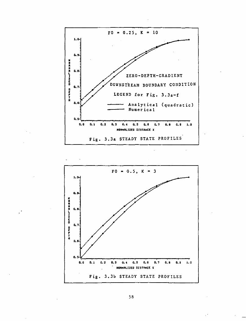
state are very good (see Fig. 3.3, 3.4).

3,4 ANALYTICAL APPROXIMATIONS TO STEADY STATE ·-

Polynomials have been adopted for most

approximations in this section because of the relative ease

in handling them during integration and differentiation. The

case for the zero-depth-gradient boundary condition is much

simpler to replicate. All the analytical expressions satisfy

the boundary conditions i.e. matching slopes at both ends x

= 0 and x = 1. The complete behaviour of the steady state is

known at the lower boundary. The curvature and higher

derivatives at this point may be determined by succesive

differentiation of the governing equation.

Among the many polynomials tried, the cubic which

matches the slope at x = 0 and the ordinate, slope a~d

57

• a • •

J.

0.9

• a.a L I z £ D

D £ • r

"

• a • "

a. 7

I.

0.

• •• L I z £ D

D £ • r

"

D. 7

o.

FO = 0.25, K = 10

~/,/

.,/.,,.,-: ZERO-DEPTH-GRADIENT

/")' DOWNSTREAM BOUNDARY CO!IDITION

.,~ LEGEND for Fig. 3. 3a-f

Analytical (quadratic) Numerical

o. o o.. 1 a. 2 a., a. t a. s o. s o. 1 o. e o. 9 1. o NannALJZED DISTAMCf x

Fig. 3.3a STEADY STATE PROFILES

FO = 0.5, K 3 3

a.a 0.1 0..2 a., a.to.so.& 0.1 a.a o.9 1.0 NGftNALlZED Dl,TRNCE X

Fig. 3.3b STEADY STATE PROFILES

58

• • "

1.00

0.95

0.90

N 0..85 • L 1 z a.ea E Q

D 0.15 E , T

"

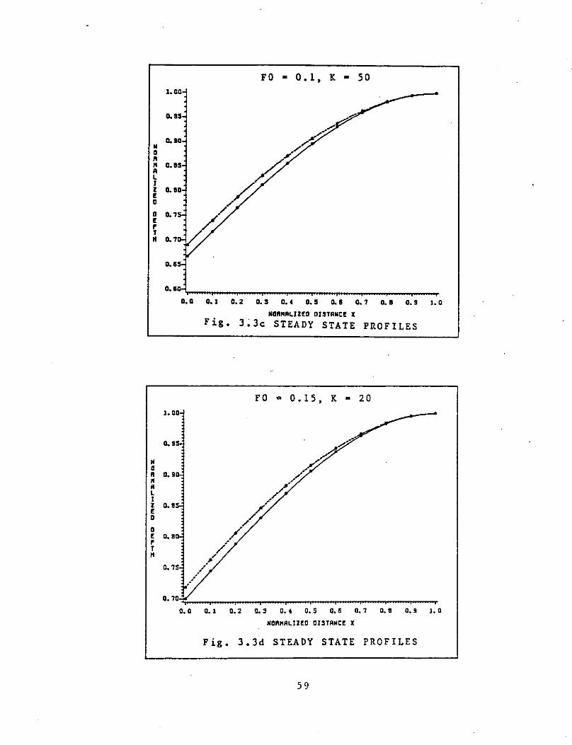
FO • 0.1, K = 50

D.Q D .. 1 D.2 0.3 0..4 0.5 O.S 0.7 0.1 0.9 J.D

NGft"A~JZ!D ot,TANC! X Fig. J;Jc STEADY STATE PROFILES

FO O 0.15, K = 20 1. 00

• • " • • L I l 0. 85 E D

D E o •• , T H

0.15

a. o o. 1 o. 2 a. 3 o. , o. s o. s a. 1 a. e o. !I 1. o NCRNA~IZED DISTANCE X

Fig. J.Jd STEADY STATE PROFILES

59

• a " " A l I l

' 0

D

' p T •

N • " " A L I l f 0

D f p I

"

J.QD

J. 2

Q. 9

Q.

o ••

Q.Q

-0.3

-o. 6

-0.9

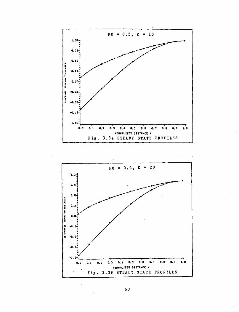
FO s 0.5, K = 10

o.o 0 .. 1 0.2 a., a., o.s o.s o.7 a.e o.s i.o NGftNALIZfD DJ3T~NC! X

Fig. 3.3e STEADY STATE PROFILES

FO = 0.4, K = 20

-----------/--/

D. D D. I Q. 2 O. 3 0. 4 D. 5 D. 6 D. 7 D. S D. 9 J. D

NGftNALJZfD DJ,TANCf X

Fig. 3.3f STEADY STATE PROFILES

60

M 0 ft • A L I z f D

D f r T •

M 0 ft • A L I z f D

D f r T •

I. 0

0.1

0.1

0.1

0.1

o. 5

0..

CRITICAL FLOW

DOWNSTREAM BOUNDARY CONDITION , ,...........-

LEGEND for Fig. 3.4a

' ' FO = 1 • K = 3 • • FO = 0.707, K =

FO = 0.4, K = 20

~a ~· L2 L3 Lt LS LS a., LI LS 1.D Natl"ALJZ£D DJ3TAMC£ X

3

Fig. 3.4a NUMERICAL STEADY STATE PROFILES

I. 0

0.9

0.1

0.1

0.1

o. LEGEND for Fig. 3.4b

• • " . FO = 1, K = 1, 5 FO = 0.5, K = 10 FO = 0.75, K = 4

D,o-,,.._..,.._...,.. _ _,. _ _,._...,._-. _ _, _ _, _ __,_-.. 0. 0 O. I O. 2 O. 3 0. < O. 5 O. I O. 1 O. I O. 9 I. 0

NDftNALIZfO OJ3TRNCf i

Fig. 3.4b NUMERICAL STEADY STATE PROFILES

61

FO = 0. 2 5, K • 10

a.a

/_...,....,.- --a., .......

• \ 0 \ • .. ,

\ • a . /" \ A L \ I i / \ ' a. I D LEGEND for Fig. J,4c-f ' D \ ' Analytical(Taylor series) , a.,~ T --- Numerical •

a.

0..0 0.1 0.2 0.3 0.4. 0.5 D.S D.1 0..8 0.9 J.O

NDftNALJZfO QJ3TANCf X

Fig, J.4c STEADY STATE PROFILES

FO a 0.15, K = 20

a.

• \ 0 \ ft a. • A I L I I • i a. \ ' • D \

a \

' a.• \ , T

" o.

a. a o. 1 a. 2 o.. , o. , o. s o. s o. 1 o. e a.. s 1. o NDRNALIZfD DJ3TANCf X

F . J,4d STEADY STATE PROFILES ig.

62

• a

0.

0.1

ft 0. • A L I z o. ! D

0 ! 0.. p T •

0.

FO = 0.1, K = 50

\ \ \

\ i i l

\ 0.2..,_~ ..... ~ ..... --~ ................................ ~ ..... ~ ..... --~ ..... --.

• a ft

1.1

1. so

" 1.,s A L I l 1. OD ! 0

Q E p T H 0.5

0.2

~o ~1 ~2 ~l o.t ~s ~s ~1 ~• o.9 1.0

NDftNALJZED DJ,TANCE X

Fig. 3.4e STEADY STATE PROFILES

FO = 0.4, K = 20

0.0 0.1 0.2 0.3 D.t 0.5 O.& 0.1 0.1 0.9 1.0

N~ftNRLJZ~D Dl~TRNC[ X

Fig. 3.4f STEADY STATE PROFILES

63

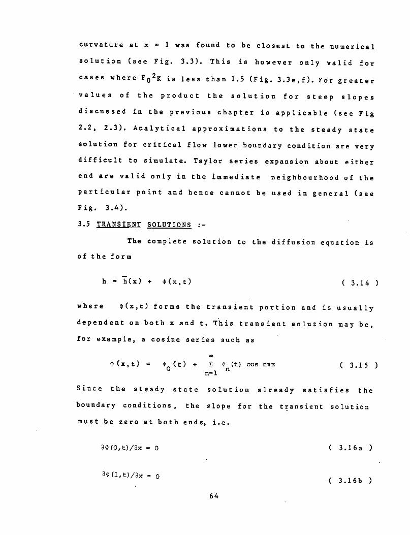
curvature at x = 1 was found to be closest to the numerical

solution (see Fig. 3.3). This is however only valid for

cases where F 0 2K is less than 1.5 (Fig. 3.3e,f). For greater

values of the product the solution for steep slopes

discussed in the previous chapter is applicable (see Fig

2.2, 2.3), Analytical approximations to the steady state

solution for critical flow lower boundary condition are very

difficult to simulate. Taylor series expansion about either

end are valid only in the immediate neighbourhood of the

particular point and hence cannot be used in general (see

Fig. 3.4).

3.5 TRANSIENT SOLUTIONS :-

The complete solution to the diffusion equation is

of the form

h = h(x) + <P(x,t) ( 3.14 )

where <P(x,t) forms the transient portion and is usually

dependent on both x and t. This transient solution may be,

for example, a cosine series such as

<l>(x,t) = i:: n=l

<P (t) n

cos n1rx ( 3.15 )

Since the steady state solution already satisfies the

boundary conditions, the slope for the transient solution

must be zero at both ends, i.e.

H(O,t)/ax = o ( 3.16a)

a~(l,t)/3x = O ( 3.16b )

64

The initial condition for the transient reduces to

equation (3,17) after simplification

~(x,O) = ~o(O)+E n=l

~ (0) cos nnx = -h(x) n

( 3.17 )

Considering a one term approximation for the transient, we

have

( 3.18 )

which means that the initial condition is satisfied for at

least one point in [0,1] from the mean value theorem. There

is an error in such an approximation, but this can be

improved upon by considering more terms in the transient and

satisfying the initial condition at more points. Following

the procedure outlined in section 2.2, i.e. integrating the

residual over the interval [0,1] converts the problem to an

initial value problem. This solution mode has been

investigated for the zero-depth-gradient condition and the

results for the outflow hydrograph are in close agreement

with the corresponding numerical solutions (see Fig.3.5),

There is an error caused at x = 0 due to considering only

one term, The scope and applicability of this solution

procedure are discussed in the next chapter, The scheme

developed in this section is not applicable to flows with

critical depth at the downstream end.

65

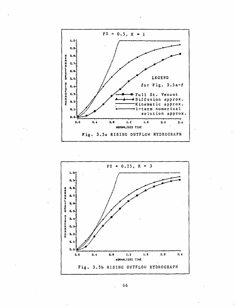
J. 0

o.s

N O. I a " " o. 7 A L I o. l ! 0 o.s D J o.' s c H o •• A

" ' o. 2 !

O. I

o.

I.

0.

• o. a

" " A L J o. l ! D O.

D I o. s c H O • • " G !

o. 0

•• 0

FO = 0. 5, K = l

/ .....-·

LEGEND

for Fig. 3.5a-f

• Full St. Venant ... 'Diffusion approx.

Kinematic: approx. 1-term numerical

solution approx.

.. ' o •• I. 2 J. S 2. 0 2.'

NGMALI?ED TINE

Fig. 3.5a RISING OUTFLOW HYDRO GRAPH

FO = 0.25, K • 3

-------

o.' o •• I. 2 I. S 2. 0 2 ••

HCANAlJZEO TJHf

Fig. 3.5b RISING OUTFLOW HYDROGRAPH

66

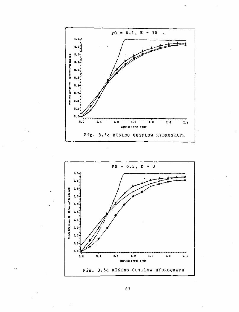
FO • 0.1, K • 50 1. a

a.s

• a.• a " ~ a., A L I a. s z f 0 a.s a I a.•

' c H a.' A ft G a.2 •

a.1~ a. a

a. a a.. a.• 1. 2 l. s 2. a 2 ••

Fig, 3.Sc RISING OUTFLOW HYDROGRAPH

FO = 0.5, K = 3

1. a r a.s I I

I • a • / • " I/, ~ A 1~/ L I o. z

./#/ • a o. a I 7/ I ' c 11 H o. A

" G a. 2 • II/ . D. I //

/,.

o. a o. 0 o •• o •• 1. 2 1. 6 2, 0 2,.

NGMALlZEO TI"I!:

Fig. J,Sd RISING OUTFLOW HYDROGRAPH

67

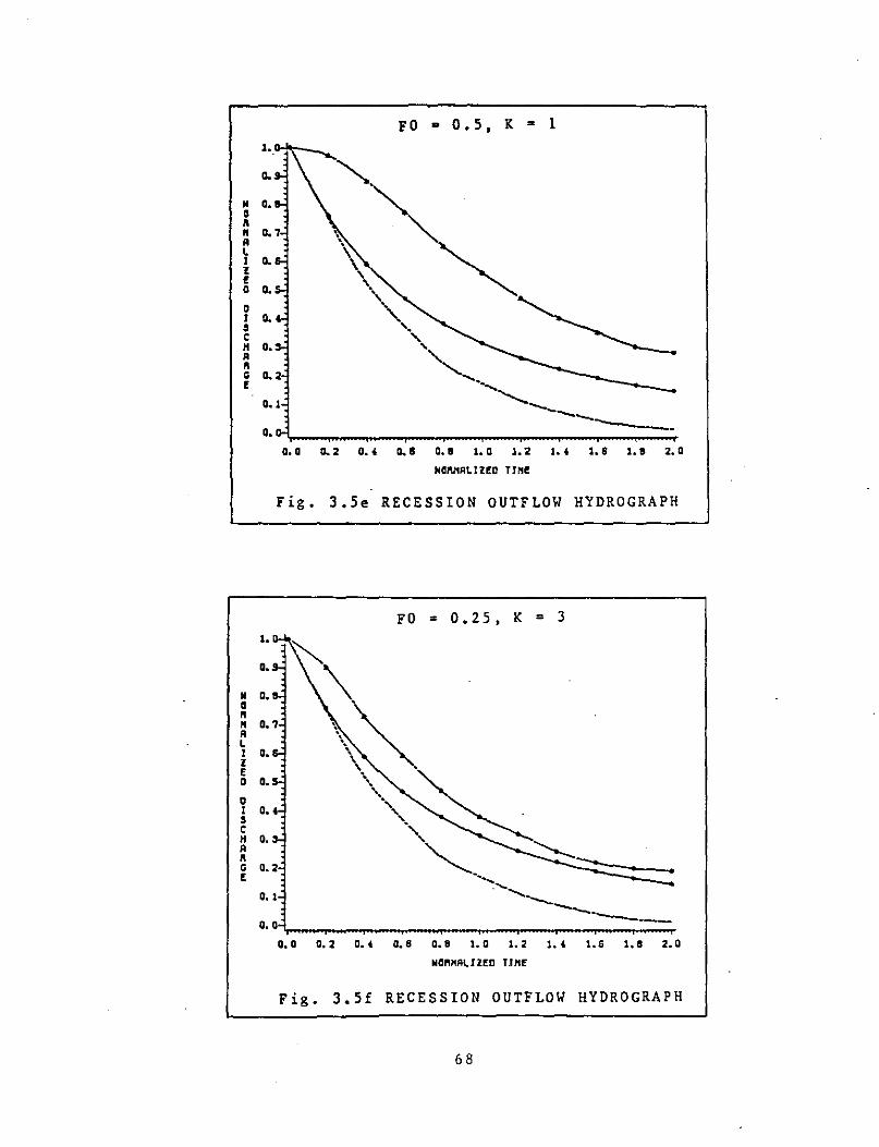
FO • o.s. K = 1 1.

0.

• a • 0

" " A L I a. I ! D a. Q l 0.

' c H a. A

" ; 0. 2 !

0.1

a. a. a 0.2 o., o.s o.e 1.0 1.2 1., 1.s 1.1 2.a

NClft;otRlIZfO TIN!

Fig, 3,5e RECESSION OUTFLOW HYDROGRAPH

1.

a.

• a. a " " A L I D. I E O c. 0 I D.

' c H D. A

" G Q. 2 E

Q, I

FO = 0.25, K = 3

•

a.a 0.2 a., a.s a.e 1.0 1.2 1., 1.s 1.a 2.0 NCl"NAlJZfD T.INE

Fig, 3.5f RECESSION OUTFLOW HYDROGRAPH

68

CHAPTER!~ DISCUSSION !Jill. CONCLUSIONS

4,1 DISCUSSION ·-

~ good numerical scheme is one which is stable and

converges rapidly. Non-linear systems of differential

equations frequently involve the solution of non linear

simultaneous equations. Most schemes for solving such a

system use a variant of Newton's method and are economical

if convergence is achieved within a couple of iterations.

Some researchers have found it preferable to use Richtmyer's

algorithm or the 'double sweep method' which involves the

inversion of a 2 * 2 matrix for which expressions can be

written directly,

Both the method of characteristics and finite

difference schemes are acceptable techniques. They suffer

from the disadvantage of involving long and formidable

equations. Their stability can be ensured by using

appropriate time steps and space discretization. The series

solutions discussed in the text are very simple to formulate

and convergence is very rapid. For most cases two terms are

adequate. The many instances considered show that this

scheme performs very well (see Fig. 2.2, 2.3). It is an

69

entirely new solution procedure adopting a different

approach to the problem and is therefore important in its

own right. It has all the properties of a good numerical

solution.

Analytical solutions developed by previous

researchers involve linearization of the differential

equation (usually through regular perturbations). The

analytical procedure described in the text preserves the

non-linearity in the problem to a greater extent. The system

of non-linear equations solved for preparing TABLE 2.1 are

solved only once for each combination of F 0 and Kand may be

used for later work.

It is clear from this study that the zero-depth­

gradient at the downstream is a much simpler condition to

handle than the critical flow requirement at the lower end.

The concept of breaking up the solution procedure into two

parts is reasonable when the physical system represented by

the differential equation reaches a steady state. A

difficult problem may

the solutions of two

therefore be solved by superimposing

simpler ones. Polynomials cannot

capture the steep behaviour of the steady state profiles in

cases of critical flow downstream boundary condition (see

Fig 3.4). Bence superimposing the transients also becomes

difficult because the initial condition for the transient

components are determined by the steady sta~e.

The diffusion wave theory is superior to the

kinematic wave though it is more difficult to solve, The

70

insensitivity of the kinematic wave to the field conditions

and its inability to account for backwater effects are among

its severe drawbacks. Therefore it cannot be used with

complete confidence in problems of channel networks. Hence a

solution which is simple in structure and can incorporate

the effect of Fo and K is a signicant contribution to this

field.

4.2 CONCLUSIONS :-

The diffusion wave is too difficult a problem to

attempt a blanket solution for all cases using the Fourier

series approach. Hence different solution procedures were

adopted for steep slopes and mild slopes. Sin~e the

kinematic wave is just a single profile a simple solution is

feasible in this instance.

The diffusion wave is known to perform well for

small Fo and large K. A large value of K usually indicates

steep bed slopes and the solution discussed in section 2.2

is applicable in such cases. The performance of the solution

indicates that the boundary condition of zero depth at the

upstream produces similar outflow profile to the one

produced by the zero influx upper end condition (see Fig.

2.2, 2.3). Physically this implies that not much water

accumulates at the beginning of the ovezland flow plane for

such cases. An inspection of the steady state profiles shows

that the depth at x = 0 is practically zero for cases of

Fo2K greater than 1.5 (Fig. 3.3e,f, 3.4e,f). Hence the

solution procedure of section 2.2 may be used under the

71

condition stated above. It may be noted here that the zero­

depth-gradient condition is valid for large vaues of Fo 2 K.

However the Diffusion wave is a good approximation for small

Fo ( < 0.5 ) and large K ( > 10 ,say).

It may also be observed that the upstream boundary

condition has little or no effect on the outflow

hydrographs. For important problems like channel networks

and catchment-stream problems it is the profile at the

outflow section of the overland flow plane that is of

primary significance. The efforts of most previous

researchers have been concentrated in this phase of the

solution. Therefore, when the profile at x = 1 is of

interest, the solution procedure outlined in section 2.2 may

be used for all those cases where the zero-depth-gradient

downstream is a valid approximation.

The analytical expression (obtained as an

approximate solution for steep slopes) is found to perform

very well in the neighbourhood of the steady state

(Fig.2.3). The recession profiles beginning close to the

steady state are more accurate as a result. For design

purposes, the most critical piofiles are of major interest.

This implies that the full profile needs to be developed

before the recession starts. The steady state would

therefore seem to be a good indicator of peak flood

discharge and the analytical expression (discussed in

section 2.3) may be employed in such cases.

Section 3.4 deals with the steady state solution

72

procedure for cases where F 0 2K is less than 1.5 and when

zero-depth-gradient downstream end condition and zero-inflow

upstream boundary condition are used (see Fig 3.3). This

therefore covers all cases for this end condition. The case

for critical flow at x = l is not amenable to a solution of

this form because the steady state has very steep slope

requirements and cannot be matched by using polynomials

(Fig. 3 • 4).

The steady state analysis reveals several

interesting features. Complete knowledge of the behaviour of

the steady state solution at the outflow section is

obtained. For the zero-depth-gradient condition,· the· steady

state reaches its maximum normalized depth of 1.0 here.

However the critical flow downstream boundary requirement

yields a different profile. The maximum does not occur at x

= 1 because of the severe negative slope at that end. The

case for Fo = 1 reduces identically to the zero-depth­

gradient condition for all values of K as far as the steady

state profile is concerned.

The key variable in both kinematic and diffusion

approximations is K. The smplification of the momentum

equation is valid only for large K. For smaller values of K

(say K < 5), the terms in the momentum equation are not

negligible. Hence, results for greater values of Kare found

to be better than those for smaller K (see Fig. 2.2). It may

be noticed that the kinematic wave approximation naturally

satisfies the zero-depth-gradient downstream boundary

73

condition and the zero depth condition at x = 0. Therefore

it is analogous to the case of Fo = 1. This is phys'.cally

reasonable since the kinematic wave works well for steep bed

slopes on which the flows are close to being critical.

74

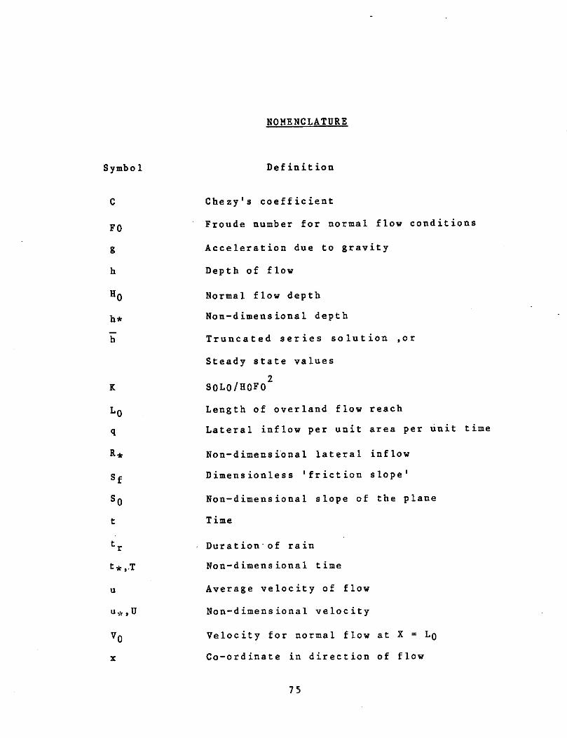
Symbol

c

FO

g

h

Ho

h*

h

u

u~':, U

x

NOMENCLATURE

Definition

Chezy's coefficient

Froude number for normal flow conditions

Acceleration due to gravity

Depth of flow

Normal flow depth

Non-dimensional depth

Truncated series solution ,or

Steady state values

2 SOLO/HOFO

Length of overland flow reach

Lateral inflow per unit area per unit time

Non-dimensional lateral inflow

Dimensionless 'friction slope'

Non-dimensional slope of the plane

Time

Duration of rain

Non-dimensional time

Average velocity of flow

Non-dimensional velocity

Velocity for normal flow at X = Lo

Co-ordinate in direction of flow

75

Symbol

y

·fl

p

e

NOMENCLATURE(Contnd.)

Definition

Non-dimensional x

Momentum correction factor

Specific weight of water

l/Fo2K

Manning's coefficient

Density of water

Angle of slope

76

REFERENCES

Amein, Michael. (1968): "An Implicit Method for Numerical Flood Routing". Water Resources Research, Vol. 4, No. 4, August, pp. 719-726.

Beven, K. (1979): Routing Method". pp 1238-1242.

"0 n Water

The Generalized Kinematic Resources Research, 15(5),

Bronson, Richard. (1973): "Modern Introductory Differential Equations". Schaum's Outline Series in Mathematics, McGraw­Hill Book Company.

Brutsaert, Wilfried. (1968): "The Initial Phase of the Rising Hydrograph of Turbulent Free Surface Flow with Unsteady Lateral Inflow". Water Research. Vol. 4, No.6, December, pp. 1189-1192.

Grace, R.A. and Eagleson, P.S. (1966): "The Modelling of Overland Flow". Water Resources Research. Vol. 2, No. 3, Third Quarter, pp. 393-403.

Henderson, F.M. and Wooding R.A. (1964): "Overland flow and groundwater flow from a steady rainfall of finite duration''. J. of Geophysical Res., 69, No. 8, pp. 1531-1540.

Hjelmfelt, A.T. (1981): Distributed Rainfall". ASCE,

"Overland Flow HY2, pp. 227-237,

Fr.om Time -February.

Liggett, Solutions 39-71.

J.A. and Woolhiser, D.A. (1967): "Difference of the Shallow-Water Equation". ASCE, April, pp.

Lighthill, M.J. and Whitham, G.B. (1955): "On waves. Flood movement in long rivers". Proc. London, Sec.A, Vol. 229, pp.281-316,March.

kinematic Roy. Soc.

Morris, E.M. (1978): "The Effect of The Small­Slope approximation and Lower Boundary Condition on the Solutions of The Saint-Venant Equations". Journal of Hydrology, 40(1979)31-47,July.

Morris, E.M. and Woolhiser, D.A. (1980): "Unsteady One Dimensional Flow Over a Plane: Partial Equilibrium and Recession Hydrographs''. Water Resources Research, Vol.16, No. 2, pp.355-360, April.

Par 1 an g e, J. Y., Rose, C. W. and Sander, G. ( 1980 ): "Kine mat i c Flow Approximation of Runoff on a Plane: An Exact Analytical

77

Solution". Journal of Hydrology, 52(1981)43-58, January.

Vieira, J.H.D. (1982): "Conditions Governing The Use of Approximations for the Saint-Venant Equations for Shallow Surface Waier Flow". Journal of Hydrology, 60(1983)43-58, January.

Wooding, R.A. (1965): "A Hydraulic Model For Catchment-Stream Problem. i.Kinematic-wave theory". Journal of Hydrology, 3(3):254-267.

Wooding, R.A. (1965): Catchment-Stream Problem. ii. of Hydrology, 3(3):268-282

"A Hydraulic Model For Numerical solutions". Journal

Wooding, R.A. (1965): "A Hydraulic Catchment-Stream Problem. 111. Comparison observations". Journal of Hydrology, 4(1):21-37

Model For with runoff

Woolhiser, D.A. (1974): "Unsteady Free-Surface Flow Problems". Proc. of Institute on Unsteady Flow in Open Channels, Colorado State University, July, pp. 195-213

Woolhiser, D.A. and Liggett, J.A. (1967): "Unsteady, One­Dimensional flow over a Plane- the Rising Hydrograph". Water Resources Research. Vol. 3, No. 3, Third Quarter, pp.753-771.

78

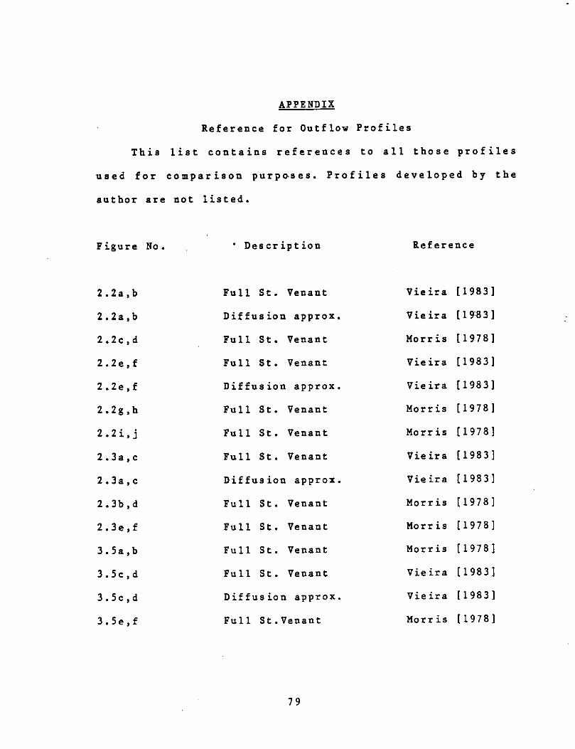
APPENDIX

Reference for Outflow Profiles

This list contains references to all those profiles

used for comparison purposes. Profiles developed by the

author are not listed.

Figure No. • Description Reference

2.2a,b Full St. Venant Vieira [1983]

2.2a,b Diffusion approx. Vieira [19'.83]

2.2c,d Full St. Venant Morris [1978]

2.2e,f Full St. Venant Vieira [1983]

2.2e,f Diffusion approx. Vieira [1983]

2.2g,h Full St. Venant Morris [1978]

2.2i,j Full St. Venant Morr is [1978]

2.3a,c Full St. Venant Vieira [1983]

2.3a,c Diffusion approx. Vieira [1983]

2.3b,d Full st. Venant Morr is [1978]

2.3e,f Full St. Venant Morris [1978]

3.Sa,b Full st . Venant Morris [1978]

3.Sc,d Full st • Ven ant Vieira [1983]

3.Sc,d Diffusion approx. Vieira [1983]

3.Se,f Full St.Venant Morr is [1978]

79