Original citation - WRAP: Warwick Research Archive Portalwrap.warwick.ac.uk/47476/13/WRAP_rawlinson-bhalerao-wang-chap-2010.pdfAbhir Bhalerao University of Warwick, UK Li Wang

warwick.ac.uk/lib-publications

Original citation: Rawlinson, T., Bhalerao, Abhir and Wang, L. (2010) Principles and methods for face recognition and face modelling. In: Li, Chang-Tsun, (ed.) Handbook of research on computational forensics, digital crime and investigation : methods and solutions. IGI Global, pp. 53-78. ISBN 9781605668369 Permanent WRAP URL: http://wrap.warwick.ac.uk/47476 Copyright and reuse: The Warwick Research Archive Portal (WRAP) makes this work by researchers of the University of Warwick available open access under the following conditions. Copyright © and all moral rights to the version of the paper presented here belong to the individual author(s) and/or other copyright owners. To the extent reasonable and practicable the material made available in WRAP has been checked for eligibility before being made available. Copies of full items can be used for personal research or study, educational, or not-for-profit purposes without prior permission or charge. Provided that the authors, title and full bibliographic details are credited, a hyperlink and/or URL is given for the original metadata page and the content is not changed in any way. A note on versions: The version presented in WRAP is the published version or, version of record, and may be cited as it appears here. For more information, please contact the WRAP Team at: [email protected]

http://go.warwick.ac.uk/lib-publications

http://go.warwick.ac.uk/lib-publications

http://wrap.warwick.ac.uk/47476

mailto:[email protected]

53

Copyright © 2010, IGI Global. Copying or distributing in print or electronic forms without written permission of IGI Global is prohibited.

Chapter 3Principles and Methods for Face Recognition and Face Modelling

Tim RawlinsonWarwick Warp Ltd., UK

Abhir BhaleraoUniversity of Warwick, UK

Li WangWarwick Warp Ltd., UK

INTRODUCTION

Face recognition is such an integral part of our lives and performed with such ease that we rarely stop to consider the complexity of what is being done. It is the primary means by which people identify each other and so it is natural to attempt to ‘teach’ computers to do the same. The applications of automated

AbsTRACT

This chapter focuses on the principles behind methods currently used for face recognition, which have a wide variety of uses from biometrics, surveillance and forensics. After a brief description of how faces can be detected in images, the authors describe 2D feature extraction methods that operate on all the image pixels in the face detected region: Eigenfaces and Fisherfaces first proposed in the early 1990s. Although Eigenfaces can be made to work reasonably well for faces captured in controlled conditions, such as frontal faces under the same illumination, recognition rates are poor. The authors discuss how greater accuracy can be achieved by extracting features from the boundaries of the faces by using Active Shape Models and, the skin textures, using Active Appearance Models, originally proposed by Cootes and Talyor. The remainder of the chapter on face recognition is dedicated such shape models, their implementation and use and their extension to 3D. The authors show that if multiple cameras are used the 3D geometry of the captured faces can be recovered without the use of range scanning or structured light. 3D face models make recognition systems better at dealing with pose and lighting variation.

DOI: 10.4018/978-1-60566-836-9.ch003

54

Principles and Methods for Face Recognition and Face Modelling

face recognition are numerous: from biometric authentication; surveillance to video database indexing and searching.

Face recognition systems are becoming increasingly popular in biometric authentication as they are non-intrusive and do not really require the users’ cooperation. However, the recognition accuracy is still not high enough for large scale applications and is about 20 times worse than fingerprint based systems. In 2007, the US National Institute of Standards and Technology (NIST) reported on their 2006 Face Recognition Vendor Test – FRVT – results (see [Survey, 2007]) which demonstrated that for the first time an automated face recognition system performed as well as or better than a human for faces taken under varying lighting conditions. They also showed a significant performance improvement across vendors from the FRVT 2002 results. However, the best performing systems still only achieved a false reject rate (FRR) of 0.01 (1 in a 100) measured at a false accept rate of 0.001 (1 in one thousand). This translates to not being able to correctly identify 1% of any given database but falsely identify 0.1%. These best-case results were for controlled illumination. Contrast this with the current best results for fingerprint recognition when the best performing fingerprint systems can give an FRR of about 0.004 or less at an FAR of 0.0001 (that is 0.4% rejects at one in 10,000 false accepts) and this has been benchmarked with extensive quantities of real data acquired by US border control and law enforcement agencies. A recent study live face recognition trial at the Mainz railway station by the German police and Cognitec (www.cognitec-systems.de) failed to recognize ‘wanted’ citizens 60% of the time when observing 23,000 commuters a day.

The main reasons for poor performance of such systems is that faces have a large variability and repeated presentations of the same person’s face can vary because of their pose relative to the camera, the lighting conditions, and expressions. The face can also be obscured by hair, glasses, jewellery, etc., and its appearance modified by make-up. Because many face recognitions systems employ face-models, for example locating facial features, or using a 3D mesh with texture, an interesting output of face rec-ognition technology is being able to model and reconstruct realistic faces from a set of examples. This opens up a further set of applications in the entertainment and games industries, and in reconstructive surgery, i.e. being able to provide realistic faces to games characters or applying actors’ appearances in special effects. Statistical modelling of face appearance for the purposes of recognition, also has led to its use in the study and prediction of face variation caused by gender, ethnicity and aging. This has important application in forensics and crime detection, for example photo and video fits of missing persons (Patterson et al., 2007).

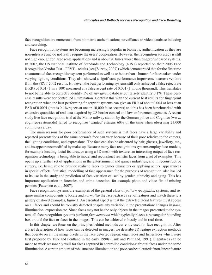
Face recognition systems are examples of the general class of pattern recognition systems, and re-quire similar components to locate and normalize the face; extract a set of features and match these to a gallery of stored examples, figure 1. An essential aspect is that the extracted facial features must appear on all faces and should be robustly detected despite any variation in the presentation: changes in pose, illumination, expression etc. Since faces may not be the only objects in the images presented to the sys-tem, all face recognition systems perform face detection which typically places a rectangular bounding box around the face or faces in the images. This can be achieved robustly and in real-time.

In this chapter we focus on the principles behind methods currently used for face recognition. After a brief description of how faces can be detected in images, we describe 2D feature extraction methods that operate on all the image pixels in the face detected region: eigenfaces and fisherfaces which were first proposed by Turk and Pentland in the early 1990s (Turk and Pentland, 1991). Eigenfaces can be made to work reasonably well for faces captured in controlled conditions: frontal faces under the same illumination. A certain amount of robustness to illumination and pose can be tolerated if non-linear feature

55


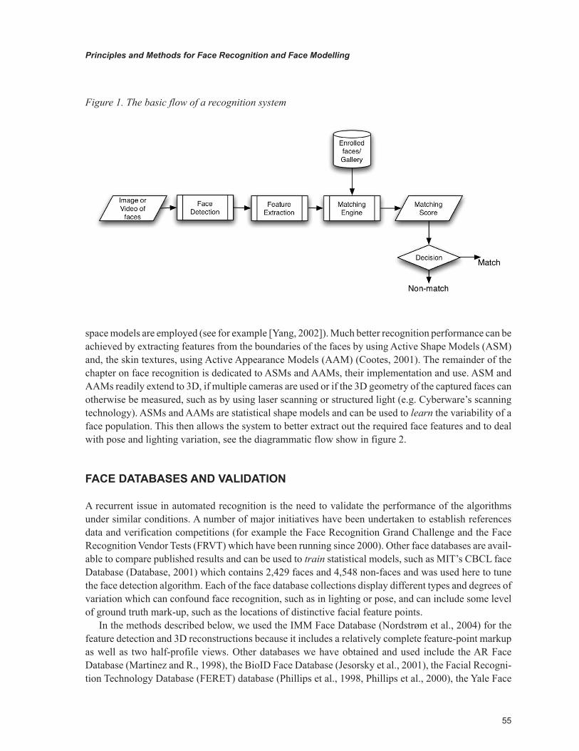
space models are employed (see for example [Yang, 2002]). Much better recognition performance can be achieved by extracting features from the boundaries of the faces by using Active Shape Models (ASM) and, the skin textures, using Active Appearance Models (AAM) (Cootes, 2001). The remainder of the chapter on face recognition is dedicated to ASMs and AAMs, their implementation and use. ASM and AAMs readily extend to 3D, if multiple cameras are used or if the 3D geometry of the captured faces can otherwise be measured, such as by using laser scanning or structured light (e.g. Cyberware’s scanning technology). ASMs and AAMs are statistical shape models and can be used to learn the variability of a face population. This then allows the system to better extract out the required face features and to deal with pose and lighting variation, see the diagrammatic flow show in figure 2.

FACE DATAbAsEs AND VALIDATION

A recurrent issue in automated recognition is the need to validate the performance of the algorithms under similar conditions. A number of major initiatives have been undertaken to establish references data and verification competitions (for example the Face Recognition Grand Challenge and the Face Recognition Vendor Tests (FRVT) which have been running since 2000). Other face databases are avail-able to compare published results and can be used to train statistical models, such as MIT’s CBCL face Database (Database, 2001) which contains 2,429 faces and 4,548 non-faces and was used here to tune the face detection algorithm. Each of the face database collections display different types and degrees of variation which can confound face recognition, such as in lighting or pose, and can include some level of ground truth mark-up, such as the locations of distinctive facial feature points.

In the methods described below, we used the IMM Face Database (Nordstrøm et al., 2004) for the feature detection and 3D reconstructions because it includes a relatively complete feature-point markup as well as two half-profile views. Other databases we have obtained and used include the AR Face Database (Martinez and R., 1998), the BioID Face Database (Jesorsky et al., 2001), the Facial Recogni-tion Technology Database (FERET) database (Phillips et al., 1998, Phillips et al., 2000), the Yale Face

Figure 1. The basic flow of a recognition system

56


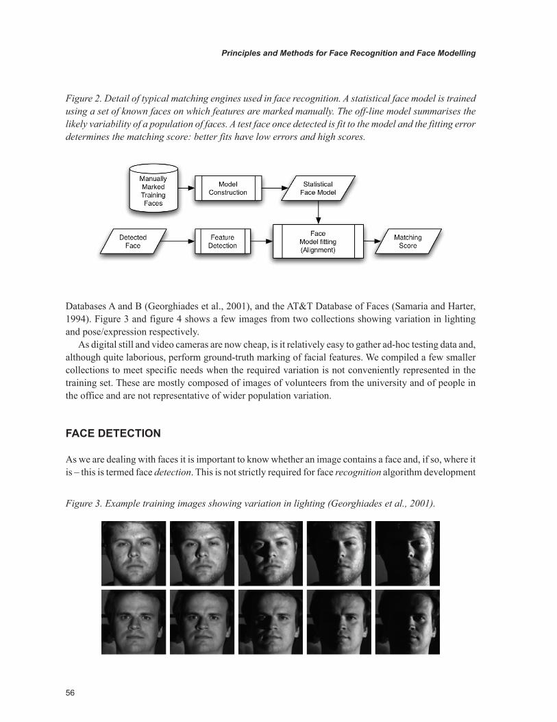
Databases A and B (Georghiades et al., 2001), and the AT&T Database of Faces (Samaria and Harter, 1994). Figure 3 and figure 4 shows a few images from two collections showing variation in lighting and pose/expression respectively.

As digital still and video cameras are now cheap, is it relatively easy to gather ad-hoc testing data and, although quite laborious, perform ground-truth marking of facial features. We compiled a few smaller collections to meet specific needs when the required variation is not conveniently represented in the training set. These are mostly composed of images of volunteers from the university and of people in the office and are not representative of wider population variation.

FACE DETECTION

As we are dealing with faces it is important to know whether an image contains a face and, if so, where it is – this is termed face detection. This is not strictly required for face recognition algorithm development

Figure 2. Detail of typical matching engines used in face recognition. A statistical face model is trained using a set of known faces on which features are marked manually. The off-line model summarises the likely variability of a population of faces. A test face once detected is fit to the model and the fitting error determines the matching score: better fits have low errors and high scores.

Figure 3. Example training images showing variation in lighting (Georghiades et al., 2001).

57


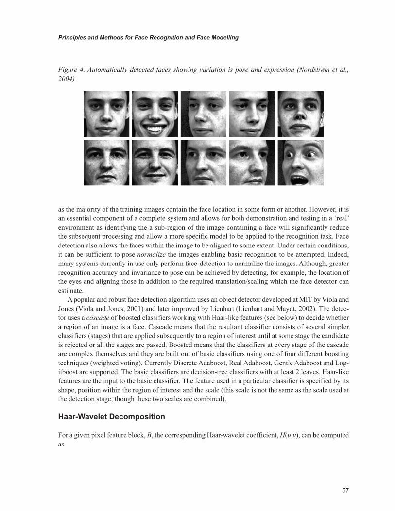
as the majority of the training images contain the face location in some form or another. However, it is an essential component of a complete system and allows for both demonstration and testing in a ‘real’ environment as identifying the a sub-region of the image containing a face will significantly reduce the subsequent processing and allow a more specific model to be applied to the recognition task. Face detection also allows the faces within the image to be aligned to some extent. Under certain conditions, it can be sufficient to pose normalize the images enabling basic recognition to be attempted. Indeed, many systems currently in use only perform face-detection to normalize the images. Although, greater recognition accuracy and invariance to pose can be achieved by detecting, for example, the location of the eyes and aligning those in addition to the required translation/scaling which the face detector can estimate.

A popular and robust face detection algorithm uses an object detector developed at MIT by Viola and Jones (Viola and Jones, 2001) and later improved by Lienhart (Lienhart and Maydt, 2002). The detec-tor uses a cascade of boosted classifiers working with Haar-like features (see below) to decide whether a region of an image is a face. Cascade means that the resultant classifier consists of several simpler classifiers (stages) that are applied subsequently to a region of interest until at some stage the candidate is rejected or all the stages are passed. Boosted means that the classifiers at every stage of the cascade are complex themselves and they are built out of basic classifiers using one of four different boosting techniques (weighted voting). Currently Discrete Adaboost, Real Adaboost, Gentle Adaboost and Log-itboost are supported. The basic classifiers are decision-tree classifiers with at least 2 leaves. Haar-like features are the input to the basic classifier. The feature used in a particular classifier is specified by its shape, position within the region of interest and the scale (this scale is not the same as the scale used at the detection stage, though these two scales are combined).

Haar-Wavelet Decomposition

For a given pixel feature block, B, the corresponding Haar-wavelet coefficient, H(u,v), can be computed as

Figure 4. Automatically detected faces showing variation is pose and expression (Nordstrøm et al., 2004)

58


H u vN u v

B S BB

i ii

NB

( , )( , )

[sgn( ) ( )],==∑1

21σ

where N(u,v) is the number of non-zero pixels in the basis image (u,v). Normally only a small number of Haar features are considered, say the first 16 × 16 (256); features greater than this will be at a higher DPI than the image and therefore are redundant. Some degree of illumination invariance can be achieved firstly by ignoring the response of the first Haar-wavelet feature, H(0,0), which is equivalent to the mean and would be zero for all illumination-corrected blocks. And secondly, by dividing the Haar-wavelet response by the variance, which can be efficiently computed using an additional ‘squared’ integral image,

I u v P x yPx

u

y

v2

1

2

1

( , ) ( , ) ,== =∑∑

so that the variance of an n × n block is

σBP P Pu vI u v

n

I u v I u v

n2

2

2 3( , )

( , ) ( , ) ( , )= −

The detector is trained on a few thousand small images (19x19) of positive and negative examples. The CBCL database contains the required set of examples (Database, 2001). Once trained it can be applied to a region of interest (of the same size as used during training) of an input image to decide if the region is a face. To search for a face in an image the search window can be moved and resized and the classifier applied to every location in the image at every desired scale. Normally this would be very slow, but as the detector uses Haar-like features it can be done very quickly. An integral image is used, allowing the Haar-like features to be easily resized to arbitrary sizes and quickly compared with the region of interest. This allows the detector to run at a useful speed (≈10fps) and is accurate enough that it can be largely ignored, except for relying on its output. Figure 4 shows examples of faces found by the detector.

Integral Image

An ‘integral image’ provides a means of efficiently computing sums of rectangular blocks of data. The integral image, I, of image P is defined as

I u v P x yx

u

y

v

( , ) ( , )== =∑∑1 1

and can be computed in a single pass using the following recurrences:

s(x,y) = s(x−1,y) + P(x,y),

I(x,y) = I(x,y − 1) + s(x,y),

59


where s(−1,y) = 0 and I(x,−1) = 0. Then, for a block, B, with its top-left corner at (x1,y1) and bottom-right corner at (x2,y2), the sum of values in the block can be computed as

S(B) = I(x1,y1) + I(x2,y2) − I(x1,y2) − I(x2,y1).

This approach reduces the computation of the sum of a 16 × 16 block from 256 additions and memory access to a maximum of 1 addition, 2 subtractions, and 4 memory accesses - potentially a significant speed-up.

IMAGE-bAsED FACE RECOGNITION

Correlation, Eigenfaces and Fisherfaces are face recognition methods which can be categorized as image-based (as opposed to feature based). By image-based we mean that only the pixel intensity or colour within the face detected region is used to score the face as belonging to the enrolled set. For the purposes of the following, we assume that the face has been detected and that a rectangular region has been identified and normalized in scale and intensity. A common approach is to make the images have some fixed resolution, e.g. 128 × 128, and the intensity be zero mean and unit variance.

The simplest method of comparison between images is correlation where the similarity is determined by distances measured in the image space. If y is a flattened vector of image pixels of size l × l, then we can score a match against our enrolled data, Gg i mi , 1≤ ≤ , of m faces by some distance measure D(y,gi), such as yTgi. Besides suffering from the problems of robustness of the face detection in cor-recting for shift and scale, this method is also computationally expensive and requires large amounts of memory. This is due to full images being stored and compared directly, it is therefore natural to pursue dimensionality reduction schemes by performing linear projections to some lower-dimensional space in which faces can be more easily compared. Principal component analysis (PCA) can be used as the dimensionality reduction scheme, and hence, the coining of the term Eigenface by Turk and Pentland (Turk and Pentland, 1991).

Face-spaces

We can define set of vectors, WT = [w1w2 … wn], where each vector is a basis image representing one dimension of some n-dimensional sub-space or ‘face space’. A face image, g, can then be projected into the space by a simple operation,

ω = −W g g( ),

where g is the mean face image. The resulting vector is a set of weights, ωT = [ω1ω2 … ωn], that de-scribes the contribution of each basis image in representing the input image.

This vector may then be used in a standard pattern recognition algorithm to find which of a number of predefined face classes, if any, best describes the face. The simplest method of doing this is to find the class, k, that minimizes the Euclidean distance,

60


∈ = −k k2 2( ) ,ω ω

where ωk is a vector describing the kth face class. If the minimum distance is above some threshold, no match is found.

The task of the various methods is to define the set of basis vectors, W. Correlation is equivalent to W = I, where I has the same dimensionality as the images.

4.1 Eigenfaces

Using ‘eigenfaces’ (Turk and Pentland, 1991) is a technique that is widely regarded as the first successful attempt at face recognition. It is based on using principal component analysis (PCA) to find the vectors, Wpca, that best describe the distribution of face images.

Let {g1, g2, … gm} be a training set of l × l face images with an average g g==∑

11m ii

m. Each im-

age differs from the average by the vector h g gi i= − . This set of very large vectors is then subject to

principal component analysis, which seeks a set of m orthonormal eigenvectors, uk, and their associated eigenvalues, λk, which best describes the distribution of the data. The vectors uk and scalars λk are the eigenvectors and eigenvalues, respectively, of the total scatter matrix,

S h h HHT ii

m

iT

m= =

=∑11

T,

where H = [h1h2 … hm].The matrix ST, however, is large (l2 × l2) and determining the eigenvectors and eigenvalues is an

intractable task for typical image sizes. However, consider the eigenvectors vk of HTH such that

HTHvi = μivi,

pre-multiplying both sides by H, we have

HHTHvi = μiHvi,

from which it can see that Hvi is the eigenvector of HHT. Following this, we construct an m × m covari-ance matrix, HTH, and find the m eigenvectors, vk. These vectors specify the weighted combination of m training set images that form the eigenfaces:

u v Hi ik kk

m

i m= ==∑1

1, ,..., .

This greatly reduces the number of required calculations as we are now finding the eigenvalues of an m × m matrix instead of l2 × l2 and in general m � l2. Typical values are m = 45 and l2 = 65,536.

61


The set of basis images is then defined as:

W u u upca nT = [ ... ],1 2

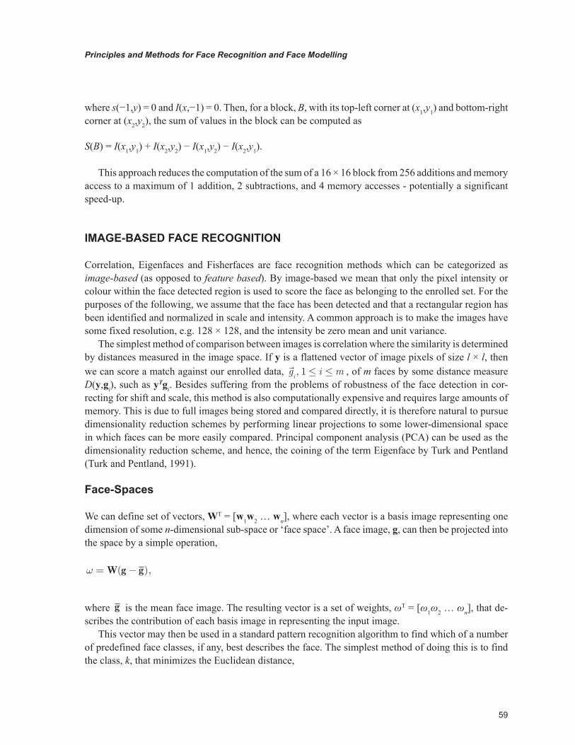
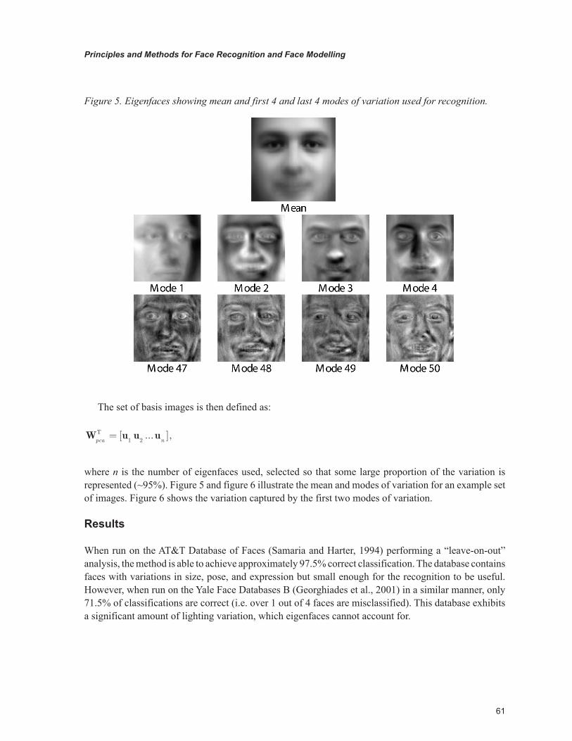
where n is the number of eigenfaces used, selected so that some large proportion of the variation is represented (~95%). Figure 5 and figure 6 illustrate the mean and modes of variation for an example set of images. Figure 6 shows the variation captured by the first two modes of variation.

Results

When run on the AT&T Database of Faces (Samaria and Harter, 1994) performing a “leave-on-out” analysis, the method is able to achieve approximately 97.5% correct classification. The database contains faces with variations in size, pose, and expression but small enough for the recognition to be useful. However, when run on the Yale Face Databases B (Georghiades et al., 2001) in a similar manner, only 71.5% of classifications are correct (i.e. over 1 out of 4 faces are misclassified). This database exhibits a significant amount of lighting variation, which eigenfaces cannot account for.

Figure 5. Eigenfaces showing mean and first 4 and last 4 modes of variation used for recognition.

62


Realtime Recognition

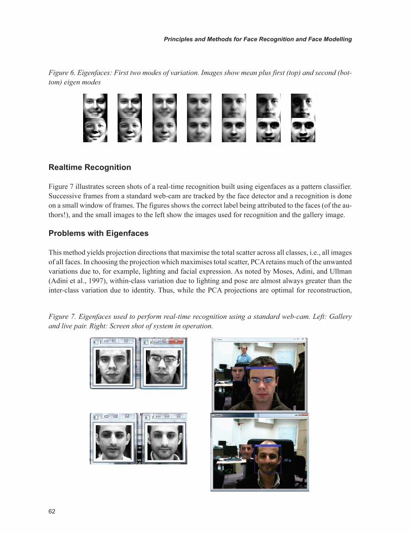
Figure 7 illustrates screen shots of a real-time recognition built using eigenfaces as a pattern classifier. Successive frames from a standard web-cam are tracked by the face detector and a recognition is done on a small window of frames. The figures shows the correct label being attributed to the faces (of the au-thors!), and the small images to the left show the images used for recognition and the gallery image.

Problems with Eigenfaces

This method yields projection directions that maximise the total scatter across all classes, i.e., all images of all faces. In choosing the projection which maximises total scatter, PCA retains much of the unwanted variations due to, for example, lighting and facial expression. As noted by Moses, Adini, and Ullman (Adini et al., 1997), within-class variation due to lighting and pose are almost always greater than the inter-class variation due to identity. Thus, while the PCA projections are optimal for reconstruction,

Figure 7. Eigenfaces used to perform real-time recognition using a standard web-cam. Left: Gallery and live pair. Right: Screen shot of system in operation.

Figure 6. Eigenfaces: First two modes of variation. Images show mean plus first (top) and second (bot-tom) eigen modes

63


they may not be optimal from a discrimination standpoint. It has been suggested that by discarding the three most significant principal components, the variation due to lighting can be reduced. The hope is that if the initial few principal components capture the variation due to lighting, then better clustering of projected samples is achieved by ignoring them. Yet it is unlikely that the first several principal components correspond solely to variation in lighting, as a consequence, information that is useful for discrimination may be lost. Another reason for the poor performance is that the face detection based alignment is crude since the face detector returns an approximate rectangle containing the face and so the images contain slight variation in location, scale, and also rotation. The alignment can be improved by using the feature points of the face.

Fisherfaces and Linear Discriminant Analysis (LDA)

Since linear projection of the faces from the high-dimensional image space to a significantly lower dimensional feature space is insensitive both to variation in lighting direction and facial expression, we can choose to project in directions that are nearly orthogonal to the within-class scatter, projecting away variations in lighting and facial expression while maintaining discriminability. This is known as Fisher Linear Discriminant Analysis (FLDA) or LDA, and in face recognition simply Fisherfaces (Belhumeur et al., 1997). FLDA require knowledge of the within-class variation (as well as the global variation), and so requires the databases to contain multiple samples of each individual.

FLDA (Fisher, 1936), computes a face-space bases which maximizes the ratio of between-class scat-ter to that of within-class scatter. Let {g1, g2, …, gm} be again a training set of l × l face images with an

average g g==∑

11m ii

m . Each image differs from the average by the vector h g gi i= − . This set of

very large vectors is then subject as in eigenfaces to principal component analysis, which seeks a set of m orthonormal eigenvectors, uk, and their associated eigenvalues, λk, which best describes the distribu-tion of the data. The vectors uk and scalars λk, are the eigenvectors and eigenvalues, respectively, of the total scatter matrix.

Consider now a training set of face images, {g1, g2, …, gm}, with average g , divided into several classes, {Χk | k = 1,…, c}, each representing one person. Let the between-class scatter matrix be defined as

S g gB kk

c

k kX X X= −( ) −( )=∑1

T

and the within-class scatter matrix as

S g gg

Wk

c

i k i kX

X Xi k

= −( ) −( )= ∈∑ ∑1

T,

64


where Xk is the mean image of class Xk and Xk is the number of samples in that class. If SW is non-singular, the optimal projection, Wopt, is chosen as that which maximises the ratio of the determinant of the between-class scatter matrix to the determinant of the within-class scatter matrix:

WW S W

W S W

u u u

optW

B

W

m

=⎛

⎝

⎜⎜⎜⎜⎜⎜

⎞

⎠

⎟⎟⎟⎟⎟⎟⎟

= ⎡⎣⎢⎤⎦⎥

argmax

...

T

T

1 2

where uk is the set of eigenvectors of SB and SW with the corresponding decreasing eigenvalues, λk, i.e.,

SBuk = λkSWuk, k = 1,…, m.

Note that an upper bound on m is c − 1 where c is the number of classes.This cannot be used directly as the within-class scatter matrix, SW, is inevitably singular. This can be

overcome by first using PCA to reduce the dimension of the feature space to N − 1 and then applying the standard FLDA. More formally,

W W W

WW W S W W

W W S W W

opt pca lda

lda W

B pca

W pca

pca

pca

=

=⎛

⎝

⎜⎜

,

argmaxT T

T T⎜⎜⎜⎜

⎞

⎠

⎟⎟⎟⎟⎟⎟

Results

The results of leave-one-out validation on the AT&T database resulted in an correct classification rate of 98.5%, which is 1% better than using eigenfaces. On the Yale Face database that contained the greater lighting variation, the result was 91.5%, compared with 71.5%, which is a significant improvement and makes Fisherfaces, a more viable algorithm for frontal face detection.

Non-Linearity and Manifolds

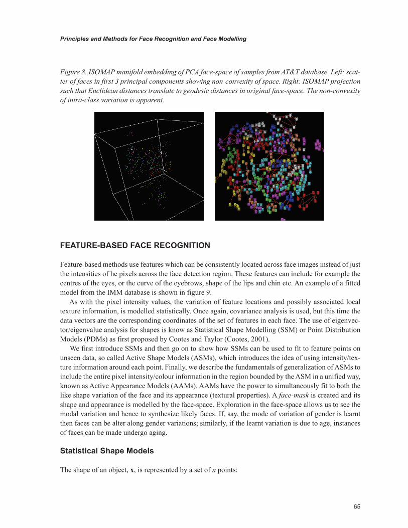
One of the main assumptions of linear methods is that the distribution of faces in the face-space is convex and compact. If we plot the scatter of the data in just the first couple of components, what is apparent is that face-spaces are non-convex. Applying non-linear classification methods, such as kernel methods, can gain some advantage in the classification rates, but better still, is to model and use the fact that the data will like in a manifold (see for example (Yang, 2002, Zhang et al., 2004)). While description of such methods is outside the scope of this chapter, by way of illustration we can show the AT&T data in the first three eigen-modes and an embedding using ISOMAP where geodesic distances in the manifold are mapped to Euclidean on the projection, figure 8.

65


FEATURE-bAsED FACE RECOGNITION

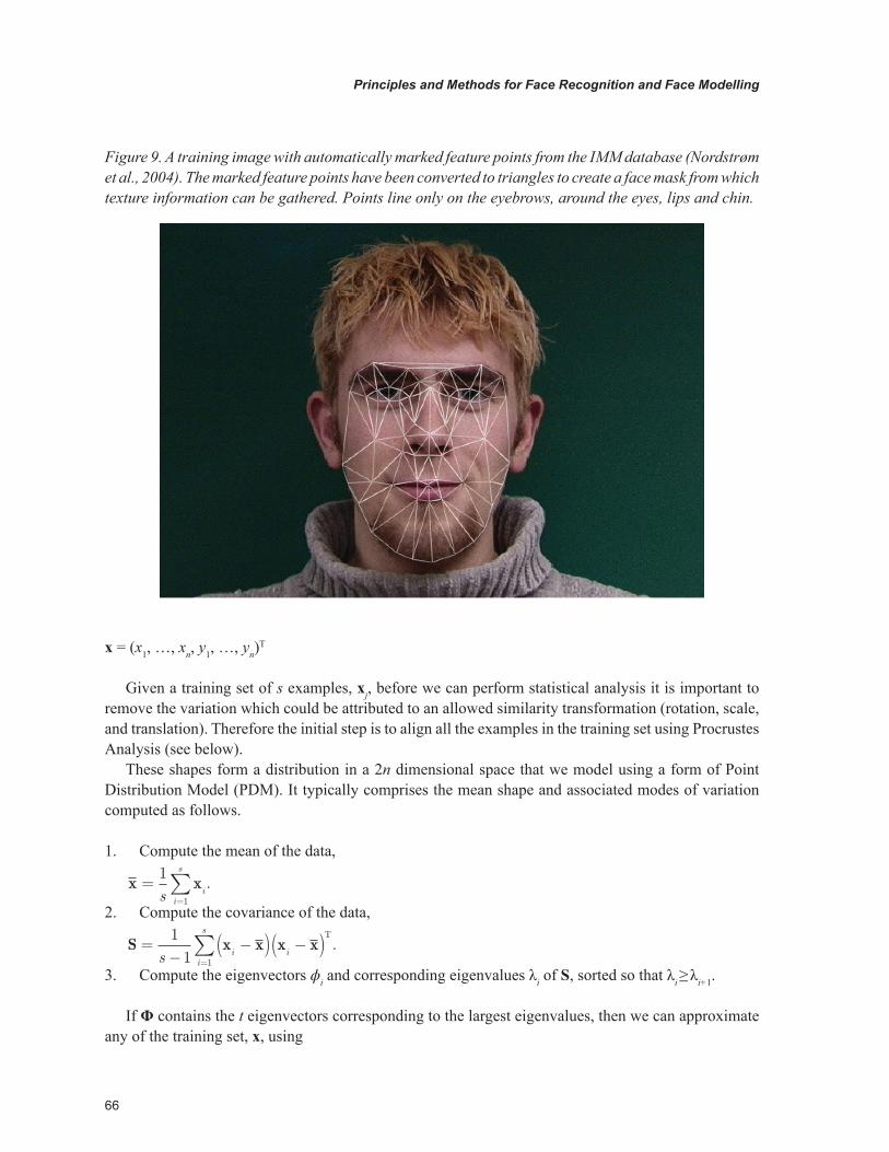
Feature-based methods use features which can be consistently located across face images instead of just the intensities of he pixels across the face detection region. These features can include for example the centres of the eyes, or the curve of the eyebrows, shape of the lips and chin etc. An example of a fitted model from the IMM database is shown in figure 9.

As with the pixel intensity values, the variation of feature locations and possibly associated local texture information, is modelled statistically. Once again, covariance analysis is used, but this time the data vectors are the corresponding coordinates of the set of features in each face. The use of eigenvec-tor/eigenvalue analysis for shapes is know as Statistical Shape Modelling (SSM) or Point Distribution Models (PDMs) as first proposed by Cootes and Taylor (Cootes, 2001).

We first introduce SSMs and then go on to show how SSMs can be used to fit to feature points on unseen data, so called Active Shape Models (ASMs), which introduces the idea of using intensity/tex-ture information around each point. Finally, we describe the fundamentals of generalization of ASMs to include the entire pixel intensity/colour information in the region bounded by the ASM in a unified way, known as Active Appearance Models (AAMs). AAMs have the power to simultaneously fit to both the like shape variation of the face and its appearance (textural properties). A face-mask is created and its shape and appearance is modelled by the face-space. Exploration in the face-space allows us to see the modal variation and hence to synthesize likely faces. If, say, the mode of variation of gender is learnt then faces can be alter along gender variations; similarly, if the learnt variation is due to age, instances of faces can be made undergo aging.

statistical shape Models

The shape of an object, x, is represented by a set of n points:

Figure 8. ISOMAP manifold embedding of PCA face-space of samples from AT&T database. Left: scat-ter of faces in first 3 principal components showing non-convexity of space. Right: ISOMAP projection such that Euclidean distances translate to geodesic distances in original face-space. The non-convexity of intra-class variation is apparent.

66


x = (x1, …, xn, y1, …, yn)T

Given a training set of s examples, xj, before we can perform statistical analysis it is important to remove the variation which could be attributed to an allowed similarity transformation (rotation, scale, and translation). Therefore the initial step is to align all the examples in the training set using Procrustes Analysis (see below).

These shapes form a distribution in a 2n dimensional space that we model using a form of Point Distribution Model (PDM). It typically comprises the mean shape and associated modes of variation computed as follows.

1. Compute the mean of the data,

x x==∑11s i

i

s

.

2. Compute the covariance of the data,

S x x x x=−

−( ) −( )=∑1 1 1s i ii

s T.

3. Compute the eigenvectors ϕi and corresponding eigenvalues λi of S, sorted so that λi ≥ λi+1.

If Φ contains the t eigenvectors corresponding to the largest eigenvalues, then we can approximate any of the training set, x, using

Figure 9. A training image with automatically marked feature points from the IMM database (Nordstrøm et al., 2004). The marked feature points have been converted to triangles to create a face mask from which texture information can be gathered. Points line only on the eyebrows, around the eyes, lips and chin.

67


x x b≈ +Φ ,

where Φ = (ϕ1| ϕ2 | … | ϕt) and b is a t dimensional vector given by

b x x= −( )ΦT .

The vector b defines a set of parameters of a deformable model; by varying the elements of b we can vary the shape, x. The number of eigenvectors, t, is chosen such that 95% of the variation is repre-sented.

In order to constrain the generated shape to be similar to those in the training set, we can simply

truncate the elements bi such that bi i≤ 3 λ . Alternatively we can scale b until

bMi

ii

t

t

2

1 λ=∑⎛

⎝⎜⎜⎜⎜⎜

⎞

⎠

⎟⎟⎟⎟⎟≤ ,

where the threshold, Mt, is chosen using the X2 distribution.To correctly apply statistical shape analysis, shape instances must be rigidly aligned to each other to

remove variation due to rotation and scaling.

shape Alignment

Shape alignment is performed using Procrustes Analysis. This aligns each shape so that that sum of

distances of each shape to the mean, D i= −∑ x x2, is minimised. A simple iterative approach is as

follows:

1. Translate each example so that its centre of gravity is at the origin.2. Choose one example as an initial estimate of the mean and scale so that x = 1 .3. Record the first estimate as the default reference frame, x0 .4. Align all shapes with the current estimate of the mean.5. Re-estimate the mean from the aligned shapes.6. Apply constraints on the mean by aligning it with x0 and scaling so that x = 1 .7. If not converged, return to 4.

The process is considered converged when the change in the mean, x , is sufficiently small.The problem with directly using an SSM is that it assumes the distribution of parameters is Gauss-

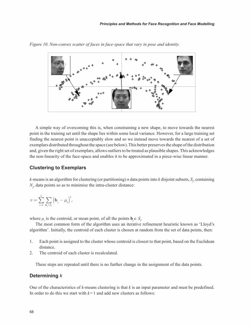
ian and that the set of of ‘plausible’ shapes forms a hyper-ellipsoid in parameter-space. This is false, as can be seen when the training set contains rotations that are not in the xy-plane, figure 10. It also treats outliers as being unwarranted, which prevents the model from being able to represent the more extreme examples in the training set.

68


A simple way of overcoming this is, when constraining a new shape, to move towards the nearest point in the training set until the shape lies within some local variance. However, for a large training set finding the nearest point is unacceptably slow and so we instead move towards the nearest of a set of exemplars distributed throughout the space (see below). This better preserves the shape of the distribution and, given the right set of exemplars, allows outliers to be treated as plausible shapes. This acknowledges the non-linearity of the face-space and enables it to be approximated in a piece-wise linear manner.

Clustering to Exemplars

k-means is an algorithm for clustering (or partitioning) n data points into k disjoint subsets, Sj, containing Nj, data points so as to minimise the intra-cluster distance:

v jSi

k

j i

= −( )∈=∑∑ b ib

µ2

1

,

where μi is the centroid, or mean point, of all the points bj ∈ Si.The most common form of the algorithm uses an iterative refinement heuristic known as ‘Lloyd’s

algorithm’. Initially, the centroid of each cluster is chosen at random from the set of data points, then:

1. Each point is assigned to the cluster whose centroid is closest to that point, based on the Euclidean distance.

2. The centroid of each cluster is recalculated.

These steps are repeated until there is no further change in the assignment of the data points.

Determining k

One of the characteristics of k-means clustering is that k is an input parameter and must be predefined. In order to do this we start with k = 1 and add new clusters as follows:

Figure 10. Non-convex scatter of faces in face-space that vary in pose and identity.

69


1. Perform k-means clustering of the data.2. Calculate the variances of each cluster:

σ µjj

jSNj

2 21= −( )

∈∑ bb

.

3. Find S0, all points that are outside d standard deviations of the centroid of their cluster in any dimension.

4. If |S0| ≥ nt then select a random point from S0 as a new centroid and return to step 1.

5.2 Active shape Models

Active Shape Models employ a statistical shape model (PDM) as a prior on the co-location of a set of points and a data-driven local feature search around each point of the model. A PDM consisting of a set of distinctive feature locations is trained on a set of faces. This PDM captures the variation of shapes of faces, such as their overall size and the shapes of facial features such as eyes and lips. The greater the variation that exists in the training set, the greater the number of corresponding feature points which have to be marked on each example. This can be a laborious process and it is hard to judge sometimes if certain points are truly corresponding.

Model Fitting

The process of fitting the ASM to a test face consists the following. The PDM is first initialized at the mean shape and scaled and rotated to lie with in the bounding box of the face detection, then ASM is run iteratively until convergence by:

1. Searching around each point for the best location for that point with respect to a model of local appearance (see below).

2. Constraining the new points to a ‘plausible’ shape.

The process is considered to have converged when either,

• the number of completed iterations have reached some limit small number;• the percentage of points that have moved less than some fraction of the search distance since the

previous iteration.

Modelling Local Texture

In addition to capturing the covariation of the point locations, during training, the intensity variation in a region around the point is also modelled. In the simplest form of an ASM, this can be a 1D profile of the local intensity in a direction normal to the curve. A 2D local texture can also be built which contains richer and more reliable pattern information — potentially allowing for better localisation of features and a wider area of convergence. The local appearance model is therefore based on a small block of pixels centered at each feature point.

70


An examination of local feature patterns in face images shows that they usually contain relatively simple patterns having strong contrast. The 2D basis images of Haar-wavelets match very well with these patterns and so provide an efficient form of representation. Furthermore, their simplicity allows for efficient computation using an ‘integral image’.

In order to provide some degree of invariance to lighting, it can be assumed that the local appear-ance of a feature is uniformly affected by illumination. The interference can therefore be reduced by normalisation based on the local mean, μB, and variance, σB

2 :

P x yP x y

NB

B

,,

.( ) = ( )− µσ2

This can be efficiently combined with the Haar-wavelet decomposition.The local texture model is trained on a set of samples face images. For each point the decomposition

of a block around the pixel is calculated. The size may be 16 pixels or so; larger block sizes increase robustness but reduce location accuracy. The mean across all images is then calculated and only a subset of Haar-features with the largest responses are kept, such that about 95% of the total variation is retained. This significantly increases the search speed of the algorithm and reduces the influence of noise.

When searching for the next position for a point, a local search for the pixel with the response that has the smallest Euclidean distance to the mean is sought. The search area is set to in the order of 1 feature block centered on the point, however, checking every pixel is prohibitively slow and so only those lying in particular directions can be considered.

Multiresolution Fitting

For robustness, the ASM itself can be run multiple times at different resolutions. A Gaussian pyramid could be used, starting at some coarse scale and returning to the full image resolution. The resultant fit at each level is used as the initial PDM at the subsequent level. At each level the ASM is run iteratively until convergence.

Active Appearance Models

The Active Appearance Model (AAM) is a generalisation of the Active Shape Model approach (Cootes, 2001), but uses all the information in the image region covered by the target object, rather than just that near modelled points/edges. As with ASMs, the training process requires corresponding points of a PDM to be marked on a set of faces. However, one main difference between an AAM and an ASM is that instead of updating the PDM by local searches of points which are then constrained by the PDM acting as a prior during training, the affect of changes in the model parameters with respect to their appearance is learnt. An vital property of the ASM is that as captures both shape and texture variations simultaneously, it can be used to generated examples of faces (actually face masks), which is a projection of the data onto the model. The learning associates changes in parameters with the projection error of the ASM.

The fitting process involves initialization as before. The model is reprojected onto the image and the difference calculated. This error is then used to update the parameters of the model, and the parameters are then constrained to ensure they are within realistic ranges. The process is repeated until the amount of error change falls below a given tolerance.

71


Any example face can the be approximated using

x x P b= +s s,

where x is the mean shape, Ps is a set of orthogonal modes of variation, and bs is a set of shape param-eters.

To minimise the effect of global lighting variation, the example samples are normalized by applying a scaling, α, and offset, β,

g = (gim − β1) /α,

The values of α and β are chosen to best match the vector to the normalised mean. Let g be the mean of the normalised data, scaled and offset so that the sum of elements is zero and the variance of elements is unity. The values of α and β required to normalise gim are then given by

α β= ⋅ = ( )g g g 1im im K, cot / .

where K is the number of elements in the vectors. Of course, obtaining the mean of the normalised data is then a recursive process, as normalisation is defined in terms of the mean. A stable solution can be found by using one of the examples as the first estimate of the mean, aligning the other to it, re-estimating the mean and iterating.

By applying PCA to the nomalised data a linear model is obtained:

g g P b= +g g,

where g is the mean normalised grey-level vector, Pg is a set of othorgonal modes of variation, and bg is a set of grey-level parameters.

The shape and appearance of any example can thus be summarised by the vectors bs and bg. Since there may be correlations between the shape and grey-level variations, a further PCA is applied to the data. For each example, a generated concatenated vector

bW bb

WP x xP g g

=⎛

⎝⎜⎜⎜⎜⎜

⎞

⎠

⎟⎟⎟⎟⎟=

−( )−( )

⎛

⎝

⎜⎜⎜⎜⎜

⎞

⎠

⎟⎟⎟⎟⎟⎟s s

g

s s

s

T

T

where Ws is a diagonal matrix of weights for each shape parameter, allowing for the difference in units between the shape and grey models. Applying PCA on these vectors gives a further model,

b = Qc,

72


where Q is the set of eigenvectors and c is a vector of appearance parameters controlling both the shape and grey-levels of the model. Since the shape and grey-model parameters have zero mean, c does as well.

Note that the linear nature of the model allows the shape and grey-levels to be expressed directly as functions of c:

x x PWQ c g g PQ c= + = +s s s g g, , (1)

where QQQ

=⎡

⎣

⎢⎢⎢

⎤

⎦

⎥⎥⎥s

g

.

Approximating a New Example

The model can be used to generate an approximation of a new image with a set of landmark points. Fol-lowing the steps in the previous section to obtain b, and combining the shape and grey-level parameters which match the example. Since Q is orthogonal, the combined appearance model parameters, c, are given by

c = QTb.

The full reconstruction is then given by applying equation (1), inverting the grey-level normalisation, applying the appropriate pose to the points, and projecting the grey-level vector into the image.

AAM Searching

A possible scheme for adjusting the model parameters efficiently, so that a synthetic example is gen-erated that matches the new image as closely as possible is described in this section. Assume that an image to be tested or interpreted, a full appearance model as described above and a plausible starting approximation are given.

Interpretation can be treated as an optimization problem to minimise the difference between a new image and one synthesised by the appearance model. A difference vector δI can be defined as,

δI = Ii −Im,

where Ii is the vector of grey-level values in the image, and Im is the vector of grey-level values for the current model parameters.

To locate the best match between model and image, the magnitude of the difference vector, Δ = |δI|2, should be minimized by varying the model parameters, c. By providing a-priori knowledge of how to adjust the model parameters during image search, an efficient run-time algorithm can be arrived at. In particular, the spatial pattern in δI encodes information about how the model parameters should be changed in order to achieve a better fit. There are then two parts to the problem: learning the relationship

73


between δI and the error in the model parameters, δc, and using this knowledge in an iterative algorithm for minimising Δ.

Learning to Model Parameters Corrections

The AAM uses a linear model to approximate the relationship between δI and the errors in the model parameters:

δc = AδI.

To find A, multiple multivariate linear regressions are performed on a sample of known model displacements, δc, and their corresponding difference images, δI. These random displacements are generated by perturbing the ‘true’ model parameters for the image in which they are known. As well as perturbations in the model parameters, small displacements in 2D position, scale, and orientation are also modelled. These four extra parameters are included in the regression; for simplicity of notation, they can be regarded simply as extra elements of the vector δc. To retain linearity, the pose is represented using (sx,sy,tx,ty), where sx = s cos (θ) and sy = s sin (θ).

The difference is calculated thus: let c0 be the known appearance model parameters for the current image. The parameters are displaced by a known amount, δc, to obtain new parameters, c = c0 + δc. For these parameters the shape, x, and normalised grey-levels, gm, using equation (?) are generated. Sample from the image are taken, warped using the points, x, to obtain a normalised sample, gs. The sample error is then δg = gs − gm. The training algorithm is then simply to randomly displace the model parameters in each training image, recording δc and δg. Multi-variate regression is performed to obtain the relationship

δc = Aδg.

The best range of values of δc to use during training are determined experimentally. Ideally, a relation-ship that holds over as large a range of errors, δg, as possible is desirable. However, the real relationship may be linear only over a limited range of values.

Iterative Model Refinement

Given a method for predicting the correction that needs to be made in the model parameters, an iterative method for solving our optimisation problem can be devised. Assuming the current estimate of model parameters, c0, and the normalised image sample at the current estimate, gs, one step of the iterative procedure is as follows:

1. Evaluate the error vector, δg0 = gs − gm.2. Evaluate the current error, E0 = |δg0|

2.3. Computer the predicted displacement, δc = Aδg0.4. Set k = 1.5. Let c1 = c0 − kδc.6. Sample the image at this new prediction and calculate a new error vector, δg1.

74


7. If |δg1| < E0 then accept the new estimate, c1.8. Otherwise try at k = 1.5, 0.5, 0.25 etc.

This procedure is repeated until no improvement in |δg0|2 is seen and convergence is declared.

AAMs with Colour

The traditional AAM model uses the sum of squared errors in intensity values as the measure to be minimised and used to update the model parameters. This is a reasonable approximation in many cases, however, it is known that it is not always the best or most reliable measure to use. Models based on intensity, even when normalised, tend to be sensitive to differences in lighting — variation in the residu-als due to lighting act as noise during the parameter update, leading optimisation away from the desired result. Edge-based representations (local gradients) seem to be better features and are less sensitive to the lighting conditions than raw intensity. Nevertheless, it is only a linear transformation of the original intensity data. Thus where PCA (a linear transformation) is involved in model building, the model built from local gradients is almost identical to one built from raw intensities. Several previous works pro-posed the use of various forms of non-linear pre-processing of image edges. It has been demonstrated that those non-linear various forms can lead AAM search to more accurate results.

The original AAM uses a single grey-scale channel to represent the texture component of the model. The model can be extended to use multiple channels to represent colour (Kittipanya-ngam and Cootes, 2006) or some other characteristics of the image. This is done by extending the grey-level vector to be the concatentation of the individual channel vectors. Normalization is only applied if necessary.

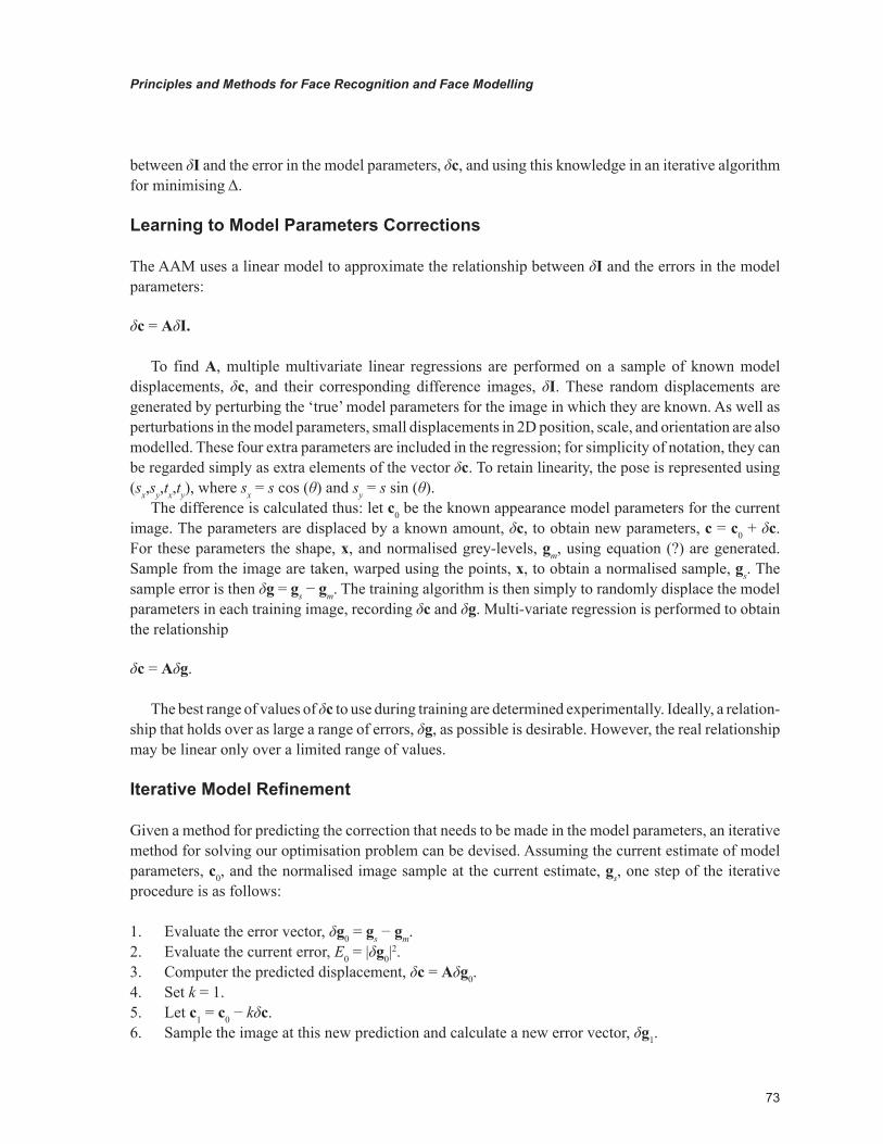
Examples

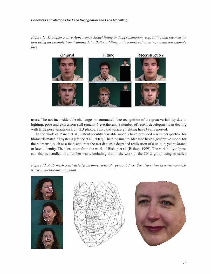
Figure 11 illustrates fitting and reconstruction of an AAM using seen and unseen examples. The results demonstrate the power of the combined shape/texture which a the face-mask can capture. The reconstruc-tions from the unseen example (bottom row) are convincing (note the absence of the beard!). Finally, figure 12 shows how AAMs can be used effectively to reconstruct a 3D mesh from a limited number of camera views. This type of reconstruction has a number of applications for low-cost 3D face recon-struction, such as building textured and shape face models for game avatars or for forensic and medical application, such as reconstructive surgery.

FUTURE DEVELOPMENTs

The performance of automatic face recognition algorithms has improved considerably over the last decade or so. From the Face Recognition Vendor Tests in 2002, the accuracy has increased by a factor of 10, to about 1% false-reject rate at a false accept rate of 0.1%. If face recognition is to compete as a viable biometric for authentication, then a further order of improvement in recognition rates is necessary. Under controlled condition, when lighting and pose can be restricted, this may be possible. It is more likely, that future improvements will rely on making better use of video technology and employing fully 3D face models, such as those described here. One of the issues, of course, is how such models can be acquired with out specialist equipment, and whether standard digital camera technology can be usefully used by

75


users. The not inconsiderable challenges to automated face recognition of the great variability due to lighting, pose and expression still remain. Nevertheless, a number of recent developments in dealing with large pose variations from 2D photographs, and variable lighting have been reported.

In the work of Prince et al., Latent Identity Variable models have provided a new perspective for biometric matching systems (Prince et al., 2007). The fundamental idea is to have a generative model for the biometric, such as a face, and treat the test data as a degraded realization of a unique, yet unknown or latent identity. The ideas stem from the work of Bishop et al. (Bishop, 1999). The variability of pose can also be handled in a number ways, including that of the work of the CMU group using so called

Figure 11. Examples Active Appearance Model fitting and approximation. Top: fitting and reconstruc-tion using an example from training data. Bottom: fitting and reconstruction using an unseen example face.

Figure 12. A 3D mesh constructed from three views of a person’s face. See also videos at www.warwick-warp.com/customization.html.

76


Eigen Light Fields (Gross et al., 2002). This work also promises to work better in variable lighting. If a fully 3D model is learnt for the recognition, such as the example 3D reconstructions shown in this chapter, then it is possible to use the extra information to deal better with poor or inconsistent illumina-tion. See for example the authors’ work on shading and lighting correction using entropy minimzation (Bhalerao, 2006).

What is already possible is to capture, to a large extent, the variability of faces in gender, ethnicity and age by the means of linear and non-linear statistical models. However, as the performance of portable devices improve and as digital video cameras are available as standard, one of the exciting prospects is to be able to capture and recognize faces in realtime, on cluttered backgrounds and irregardless of expression. Many interesting and ultimately useful applications of this technology will open up, not least in its use in criminal detection, surveillence and forensics.

ACKNOWLEDGMENT

This work was partly funded by Royal Commission for the Exhibition of 1851, London. Some of the examples images are from MIT’s CBCL (Database, 2001); feature models and 3D reconstructions were on images from the IMM face Database from Denmark Technical University (Nordstrøm et al., 2004). Other images are proprietary to Warwick Warp Ltd. The Sparse Bundle Adjustment algorithm imple-mentation used in this work is by Lourakis et al. (Lourakis and Argyros, 2004).

REFERENCEs

Adini, Y., Moses, Y., & Ullman, S. (1997). Face recognition: The problem of compensating for changes in illumination direction. IEEE Transactions on Pattern Analysis and Machine Intelligence, 19, 721–732. doi:10.1109/34.598229

Belhumeur, P. N., Hespanha, P., & Kriegman, D. J. (1997). Eigenfaces vs. fisherfaces: Recognition using class specific linear projection. IEEE Transactions on Pattern Analysis and Machine Intelligence, 19, 711–720. doi:10.1109/34.598228

Bhalerao, A. (2006). Minimum Entropy Lighting and Shadign Approximation – MELiSA. In Proceed-ings of Britsh Machine Vision Conference 2006.

Bishop, C. M. (1999). Latent variable models. In Learning in Graphical Models (pp. 371-404). Cam-bridge, MA: MIT Press.

Cootes, T. (2001). Statistical models of apperance for computer vision (Technical report). University of Manchester.

Database, C. (2001). Cbcl face database #1 (Technical report). MIT Center For Biological and Com-putation Learning.

Fisher, R. (1936). The use of multiple measurements in taxonomic problems. Annals of Eugenics, 7, 179–188.

77


Georghiades, A., Belhumeur, P., & Kriegman, D. (2001). From few to many: Illumination cone models for face recognition under variable lighting and pose. IEEE Transactions on Pattern Analysis and Ma-chine Intelligence, 23(6), 643–660. doi:10.1109/34.927464

Gross, R., Matthews, I., & Baker, S. (2002). Eigen light-fields and face recognition across pose. In Proceedings of the IEEE International Conference on Automatic Face and Gesture Recognition.

Jain, A. K., Pankanti, S., Prabhakar, S., Hong, L., Ross, A., & Wayman, J. (2004). Biometrics: A grand challenge. In Proc. of ICPR (2004).

Jesorsky, O., Kirchberg, K. J., & Frischholz, R. W. (2001). Robust face detection using the hausdorff distance. In J. Bigun & F. Smeraldi (Eds.), Proceedings of the Audio and Video based Person Authenti-cation - AVBPA 2001 (pp. 90-95). Berlin, Germany: Springer.

Kittipanya-ngam, P., & Cootes, T. (2006). The effect of texture representations on aam performance. In Proceedings of the 18th International Conference on Pattern Recognition, 2006, ICPR 2006 (pp. 328-331).

Lienhart, R., & Maydt, J. (2002). An extended set of haar-like features for rapid object detection. In Proceedings of the IEEE ICIP 2002 (Vol. 1, pp. 900-903).

Lourakis, M., & Argyros, A. (2004). The design and implementation of a generic sparse bundle adjust-ment software package based on the levenberg-marquardt algorithm (Technical Report 340). Institute of Computer Science - FORTH, Heraklion, Crete, Greece. Retrieved from http://www.ics.forth.gr/~lourakis/sba

Martinez, A., & R., B. (1998). The AR face database (CVC Technical Report #24).

Nordstrøm, M. M., Larsen, M., Sierakowski, J., & Stegmann, M. B. (2004). The IMM face database - an annotated dataset of 240 face images (Technical report). Informatics and Mathematical Modelling, Tech-nical University of Denmark, DTU, Richard Petersens Plads [Kgs. Lyngby.]. Building, 321, DK-2800.

Patterson, E., Sethuram, A., Albert, M., Ricanek, K., & King, M. (2007). Aspects of age variation in facial morphology affecting biometrics. In . Proceedings of the, BTAS07, 1–6.

Phillips, J. P., Scruggs, T. W., O’toole, A. J., Flynn, P. J., Bowyer, K. W., Schott, C. L., & Sharpe, M. (2007). FRVT 2006 and ICE 2006 large-scale results (Technical report). National Institute of Standards and Technology.

Phillips, P., Moon, H., Rizvi, S., & Rauss, P. (2000). The FERET evaluation methodology for face rec-ognition algorithms. IEEE Transactions on Pattern Analysis and Machine Intelligence, 22, 10901104. doi:10.1109/34.879790

Phillips, P. J., Wechsler, H., Huang, J., & Rauss, P. (1998). The FERET database and evaluation pro-cedure for face recognition algorithm. Image and Vision Computing, 16(5), 295–306. doi:10.1016/S0262-8856(97)00070-X

Prince, S. J. D., Aghajanian, J., Mohammed, U., & Sahani, M. (2007). Latent identity variables: Biometric matching without explicit identity estimation. In Proceedings of Advances in Biometrics (LNCS 4642, pp. 424-434). Berlin, Germany: Springer.

78


Samaria, F., & Harter, A. (1994). Parameterisation of a stochastic model for human face identification. In . Proceedings of the, WACV94, 138–142.

Sirovich, L., & Kirby, M. (1987). Low-dimensional procedure for the characterization of human faces. Journal of the Optical Society of America. A, Optics and Image Science, 4, 519–524. doi:10.1364/JOSAA.4.000519

Survey. (2007). Nist test results unveiled. Biometric Technology Today, 10-11.

Turk, M., & Pentland, A. (1991). Eigenfaces for recognition. Journal of Cognitive Neuroscience, 3(1), 71–86. doi:10.1162/jocn.1991.3.1.71

Viola, P., & Jones, M. (2001). Robust real-time object detection. International Journal of Computer Vision.

Yang, M.-H. (2002). Extended isomap for classification. In Proceedings of the 16th International Confer-ence on Pattern Recognition, 2002 (Vol. 3, pp. 615-618).

Zhang, J., Li, S. Z., & Wang, J. (2004). Manifold learning and applications in recognition. In Intelligent Multimedia Processing with Soft Computing (pp. 281-300). Berlin, Germany: Springer-Verlag.

Zuo, F., & de With, P. (2004). Real-time facial feature extraction using statistical shape model and haar-wavelet based feature search. In Proceedings of the 2004 IEEE International Conference on Multimedia and Expo, 2004, ICME ’04 (Vol. 2, pp. 1443-1446).

KEY TERMs AND DEFINITIONs

Face Recognition: Automatic recognition of human faces from photographs or videos using a database of know faces. Uses a computer vision and pattern recognition to perform matching of facial features from images to stored “templates” of know faces. Face recognition is one of a number of biometric identification methods.

Face Modelling: The process or taking 2D and 3D images of faces and building a computer model of the faces. This may be a set of facial features and their geometry; the curves of the mouth, eyes, eyebrows, chin and cheeks; or a fully 3D model which incldues depth and colour information. Face modelling can be achieved from either 2D images (static or dynamic) or using 3D range scanning devices.

Eigenimage and Eigenfaces: Face modelling using images as features of a “face space”. An early and successful form of face modelling for recognition.

Statistical Shape, Active Shape and Active Appearance Models: Statistical models of shape and colour used in computer vision. Particularly applicable and effective for face recognition problems.

Biometrics: The science of identifying someone from something they are rather than an identification card or a username/password. Types of biometrics are fingerprints, iris, faces and DNA.

Documents

Original citation - WRAP: Warwick Research Archive Portalwrap.warwick.ac.uk/47476/13/WRAP_rawlinson-bhalerao-wang-chap-2010.pdfAbhir Bhalerao University of Warwick, UK Li Wang