Power Plant Modelling Workshop at University of … · Power Plant Modelling Workshop at University of Warwick Dr. Joe Wood，Prof. Jihong Wang, Simon Caldwell, Yue Wang The Next

Power Plant Modelling Workshop at University of Warwick

Dr. Joe Wood，Prof. Jihong Wang, Simon Caldwell, Yue Wang

The Next Generation of Activated Carbon Adsorbents for the Pre-Combustion Capture of Carbon

Dioxide.

Dr Joe Wood - Introduction

◦ Project overview

◦ Modelling objectives

Simon Caldwell - Modelling of carbon capture at IGCC Power Plants

◦ Dispersion Model

◦ Adsorption Model

Yue Wang - Modelling of power plant performance

◦ Heat recovery steam generator

◦ Gas turbine and heat recovery module

General acceptance that CO2 emissions are affecting the climate

UK emissions targets for power stations is a reduction from 500 to 50 gCO2/kWhr by 2030 (1)

Up to 18 GW of investment of CCS power stations is possible in the 2020s

By 2030, 26% of global emissions from China, with 98% of power generation emissions from coal (2)

$2.7 trillion investment in power by 2030 (3)

50/50 split favouring pre-combustion to post-combustion capture (3)

1. Turner, A. et al. The Fourth Carbon Budget - Reducing emissions through the 2020s. London : Committee on Climate Change, 2010.

2. Grubb, M. Generating Electricity in a Carbon Constrained World. London : Elsevier, 2010.

3. Liang, X et al. 2011, Applied Energy, Vol. 88, pp. 1873-1885

Diagram based on Tampa Electric IGCC Process Flow Diagram, National Energy Technology Laboratory, USA http://www.netl.doe.gov/index.html

• Could provide a CO2 emission free process of the future

• Reaction to form Syngas

• Convert CO in to CO2 in water gas shift

• Separation of CO2 and hydrogen

Diagram based on Scottish Carbon Capture and Storage Centre http://www.geos.ed.ac.uk/sccs/capture/precombustion.html

University of Birmingham (Simon Caldwell)

Simulation of pre-combustion carbon capture

◦ Developing a model of the adsorption step

◦ Producing cyclic model including all PSA steps

◦ Developing model to incorporate complete carbon capture process

Incorporates adsorption isotherms, mass transfer models, fixed bed model

Unsteady state heat and mass balances

Parameter estimation from experimental data

Project Overview

CCS Process

T, P

Composition

Dry Molar Flowrate

Molecular Weight

T, P

Composition

Molar Flowrate

Molecular Weight

Fuel gas to gas turbine

Syngas from WGS Reactor

Composition: Hydrogen, Carbon dioxide, Carbon Monoxide, Nitrogen, Methane, Hydrogen Sulphide, Water

Typical PSA Process

Adsorption Purge Pressurisation

High Purity CO2

High Purity H2

Water Gas Shift Product (60% H2, 40% CO2)

Blowdown

University of Warwick ◦ Modelling and simulation study of IGCC power

generation process

Integration of power plant and CCS models ◦ Investigations of Dynamic response

Impact on power transmission and distribution network

Effect of CCS upon plant efficiency

Effect of different fuel types

Quantified analysis of the process with plant optimization







Yue Wang - Modelling of an IGCC power plant



Model being developed for the removal of CO2 from a H2/CO2 gas mixture by adsorption High CO2 content compared to post-combustion processes

High pressure – favours physisorption

Hierarchical model developed in gPROMS

Based on Axial Dispersed Plug Flow Model

Current model looks at an Adsorption system for the separation of Carbon Dioxide and Nitrogen

Literature review of CO2/N2 Adsorption Models on Zeolite 13X

Equations Component Mass Balance

Use of overall Mass balance:

Adsorption rate equation (Linear Driving Force):

Equilibrium Isotherm (Langmuir):

Temperature, Pressure and Transport Properties ◦ Thermal Operating Modes

Isothermal Adiabatic Non-isothermal

◦ Momentum Balance No pressure drop Ergun’s Equation Darcy’s Equation

◦ Mass Balance Coefficients: Mass transfer coefficient Dispersion coefficient Diffusivity

◦ Heat Balance Coefficients: Heat transfer coefficient

Fixed bed for removal of CO2 from a N2 flow

Capable of controlling pressure, input flowrates and temperature

Limited to 200°C and 25 barg

Maximum CO2 content of 25% restricted by the CO2 analyser

Main output is CO2 mole fraction

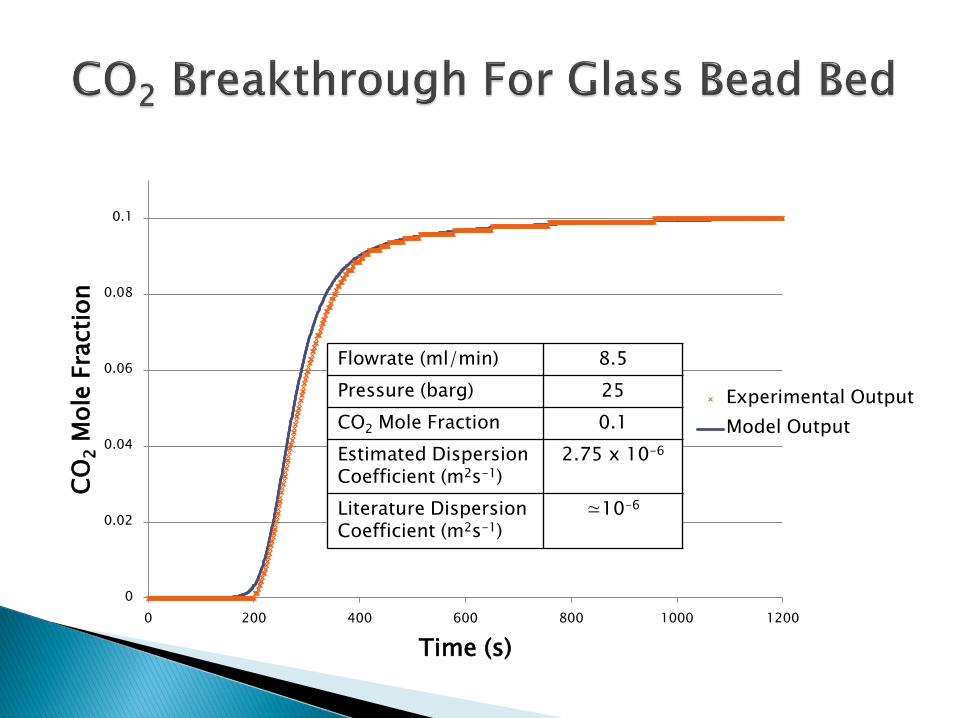
A simplified model was established where no adsorption takes place Allows ability to validate model to be tested

Tests the response of the entire experimental system

Assumes system to be isothermal with no pressure drop

Empirical models looking at response of the system without the bed were established

Experiments run with bed filled with glass beads Model Parameters identical to experiment (i.e. bed size,

flowrates etc.)

0

0.02

0.04

0.06

0.08

0.1

0 200 400 600 800 1000 1200

CO

2 M

ole

Fra

cti

on

Time (s)

Experimental Output

Model Output

Flowrate (ml/min) 8.5

Pressure (barg) 25

CO2 Mole Fraction 0.1

Estimated Dispersion Coefficient (m2s-1)

2.75 x 10-6

Literature Dispersion Coefficient (m2s-1)

≃10-6

More complex model developed for simulation of the adsorption step

Model Assumptions 1. Fluid flow is governed by axially dispersed plug flow

model 2. Equilibrium relations are given by the Langmuir

Isotherm 3. MT rates are represented by LDF equations 4. Thermal effects are negligible 5. Pressure drop represented by Ergun Equation

Parameters Estimated Dispersion coefficient, Langmuir Isotherm parameters All other parameters match experiment conditions

0

0.02

0.04

0.06

0.08

0.1

0.12

0 1000 2000 3000 4000 5000 6000 7000 8000

CO

2 M

ole

Fra

cti

on

Time (s)

Experimental Output

Model Output


Pressure (barg) 25


Bed length (cm) 7.7

Experimental Adsorption Capacity (mmol/g)

3.3

Parameters Estimated: ◦ Langmuir Isotherm Parameters:

◦ Dispersion Coefficient

Literature results vary widely for Isotherm parameters and often do not give Dispersion Coefficient values

Start point for parameter estimation severely affects estimated value Parameter Range Closest Fit

Dispersion Coefficient (m2s-1) 8.2x10-7 1.1x10-4 8.2x10-7

A (N2) (mol kg-1 Pa-1) 4.4x10-7 3.1x10-5 4.4x10-7

B (N2) Pa-1) 5.5x10-7 1.4x10-5 5.5x10-7

A (CO2) (mol kg-1 Pa-1) 1.9x10-5 6.5x10-4 1.9x10-5

B (CO2) (Pa-1) 5.4x10-6 5.0x10-4 5.4x10-6

CO2 Adsorption Capacity (mol kg-1) 1.29 3.61 3.61

Validation of estimated parameters by testing them against a shorter bed

Experiment repeated with 5g adsorbent instead of 18g, the remainder filled with glass beads All other conditions kept the same

Dispersion model used for glass bead part and adsorption model for 5g adsorbent part

Glass Beads

Zeolite 13X

CO2/N2 Mixture

0

0.02

0.04

0.06

0.08

0.1

0.12

0 500 1000 1500 2000 2500 3000 3500 4000

CO

2 M

ole

Fra

cti

on

Time (s)

Experimental Output

Model Output


Pressure (barg) 25


Bed Length (cm) 2.4

Experimental Adsorption Capacity (mmol/g)

2.8

Parameter Full Bed Best Estimate Short Bed Best Estimate

Dispersion Coefficient (m2s-1)

8.2x10-7 8.2x10-7

A (N2) (mol kg-1 Pa-1) 4.4x10-7 4.4x10-7

B (N2) Pa-1) 5.5x10-7 5.5x10-7

A (CO2) (mol kg-1 Pa-1) 1.9x10-5 4.5x10-5

B (CO2) (Pa-1) 5.4x10-6 2.5x10-5

CO2 Adsorption Capacity (mol kg-1)

3.61 1.81

Dispersion coefficients and Nitrogen Langmuir constants kept constant as they approached their bounds

Other models fit adsorption capacity closer but with significantly different parameters

Hierarchy model developed based on axial dispersed plug flow model

Simplistic dispersion only model validated

More complex adsorption model able to mimic experimental work ◦ 5 parameters estimated to give very close

approximations to experiments

Adsorption Model Improve parameter estimation

Implement energy balance

Pre-Combustion Model Switch system to using Activated Carbon adsorbent

Move towards conditions found in pre-combustion capture (i.e. Hydrogen)

Produce cyclic PSA model

Power Plant Model Complete carbon capture unit model

Combine model together with power plant model







Yue Wang - Modelling of an IGCC power plant



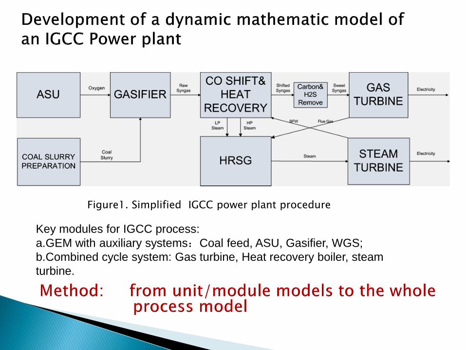
Figure1. Simplified IGCC power plant procedure

Key modules for IGCC process:

a.GEM with auxiliary systems：Coal feed, ASU, Gasifier, WGS;

b.Combined cycle system: Gas turbine, Heat recovery boiler, steam

turbine.

Pulverize coal to 5mm particles and mixed with water to feed coal slurry to the gasifier.

Coal slurry feed system

Coal mill model has been developed from our previous work.

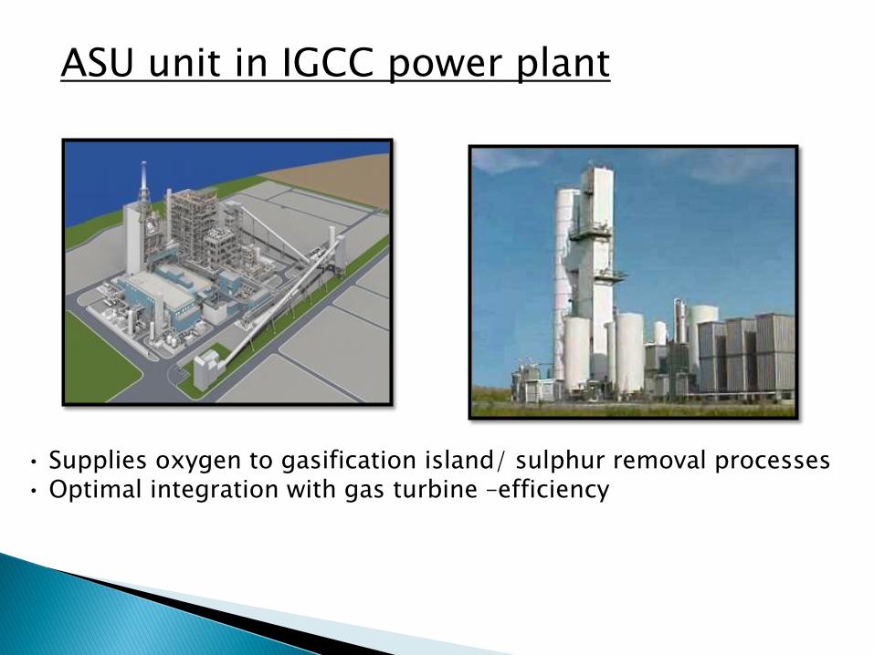
• Supplies oxygen to gasification island/ sulphur removal processes • Optimal integration with gas turbine –efficiency

ASU unit in IGCC power plant

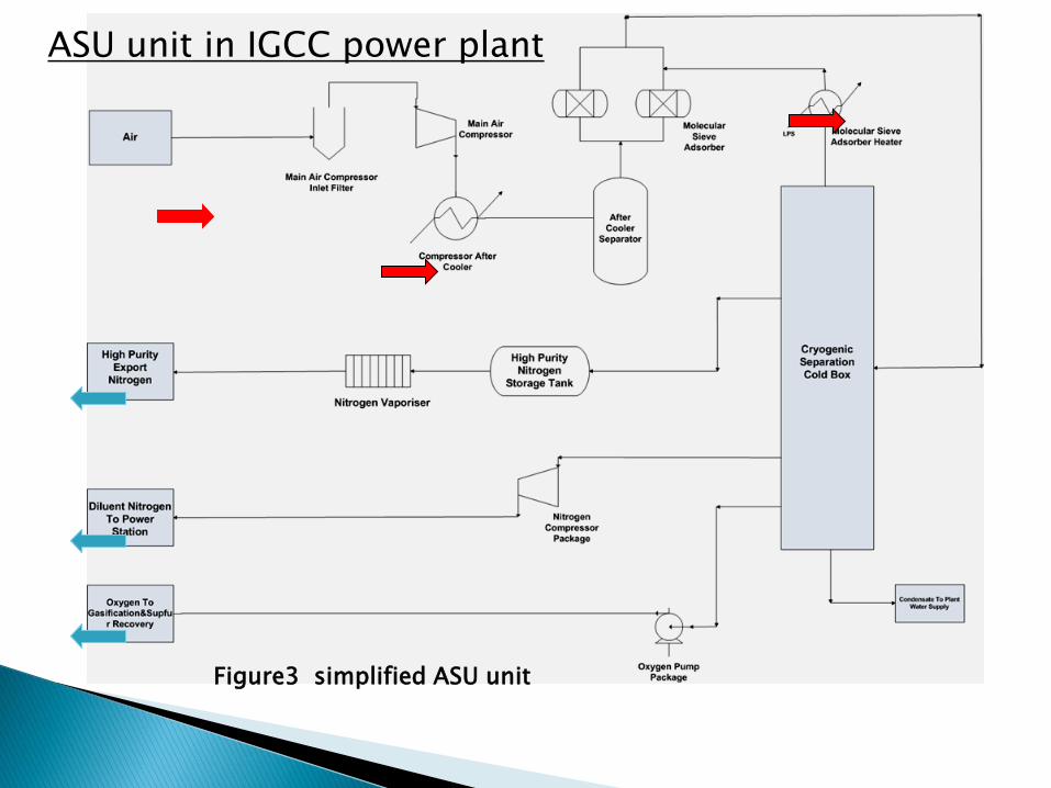
Figure3 simplified ASU unit

ASU unit in IGCC power plant

The GEM (Gasification Enabled Module )unit

• Use coal slurry oxygen and air to produce syngas; • CO shift promotes the CO2 content in syngas and prepare for the PSA removal; • Supply HP &LP steam to HRSG.

Figure 4 the GEM unit

• Main model based on gas and solid phase mass balance and energy conservation; • Chemical reaction submodel inculdes devolatilization and drying, homogeneous reactions and heterogeneous reactions; • Heat transfer submodel; • Slag layer submodel.

CO+H O CO +H -41MJ/kmol2 2 2

•Water gas shift reaction provide high partial pressure of CO2 preferred in PSA system • Improved hydrogen extraction; • Increased power output through improved gasification waste heat recovery.

• Direct contact gas / liquid exchanger where water flows against a gas

stream passing upwards； • Considerably aid waste heat recovery and lower costs, and is especially advantageous in a shifted scheme • All of the cooling train heat exchangers are liquid – liquid making them much smaller and cheaper

Gas turbine components:

Brayton cycle

Gas turbine mathematical model:

A characteristic time is used to delay the mass flow.

The Compressor (Isentropic) block increases the pressure of an incoming flow to a given outlet pressure. It determines the thermodynamic state of the outgoing flow along with the compressor's required mechanical power consumption at a given isentropic efficiency.

The realized output mass flow rate


Mixes two fluids with or without phase change. The Mixer block calculates temperature, composition and pressure after an adiabatic mixing of two fluids. The output enthalpy is the sum of the input enthalpies.

The pressure of the resulting flow

Pressure loss

K is the pressure loss factor


The Reactor block computes the outgoing flow bus (FB) after one reaction, a heat exchange with the environment and a pressure loss. Heat exchange with the surrounding environment is taken into account. In general, the outgoing flow is not in chemical equilibrium as the Reactor performs a chemical reaction depending on a rate of reaction.


The Turbine (Isentropic) block decreases the pressure of an incoming flow to a given outlet pressure. It determines the thermodynamic state of the outgoing flow along with the produced mechanical power at a given isentropic efficiency.

'3 4

3 4

oi

h h

h h

Subscripts, ‘s’ and ‘ac’ states for isentropic and actual change of state.

Turbine is adiabatic and used with gaseous flows

It is assumed, that this heat transfer rate is constant over the area of the heat exchanger or it represents a mean of the heat exchange rate.

This heat exchanger support counter flow

The Heat Exchanger block calculates the change of state of two media caused by indirect heat exchange.

To approximate the dynamic thermal behavior of the block, the heat exchanger is assumed to have a thermal mass

The heat exchange with environment is divided in four parts: both thermal masses (for flow 1 and flow 2) exchange heat with environment, both output flows exchange heat with environment. Each of the two flows entering the heat exchanger exchanges heat with its own

thermal mass, The two thermal masses are not interacting, but they have a term representing the heat exchange with environment.

• to complete the whole system modelling

• implementation of the model to software

environment;

• integrate the model with CCS process model.

Documents

Power Plant Modelling Workshop at University of … · Power Plant Modelling Workshop at University of Warwick Dr. Joe Wood，Prof. Jihong Wang, Simon Caldwell, Yue Wang The Next