Optimization of injection rates for geological CO2 storage in brine formations using EASiTool

GCCC Digital Publication Series #14-01

Seyyed A. Hosseini Seunghee Kim

Cited as: Hosseini, S.A. and Kim, S., 2014, Optimization of injection rates for geological CO2 storage in brine formations using EASiTool: presented at the 13th Annual Conference on Carbon Capture Utilization & Sequestration, Pittsburgh, Pennsylvania, April 28-May 1, 2014. GCCC Digital Publication Series #14-01.

Keywords: Capacity, Modeling-Flow simulation

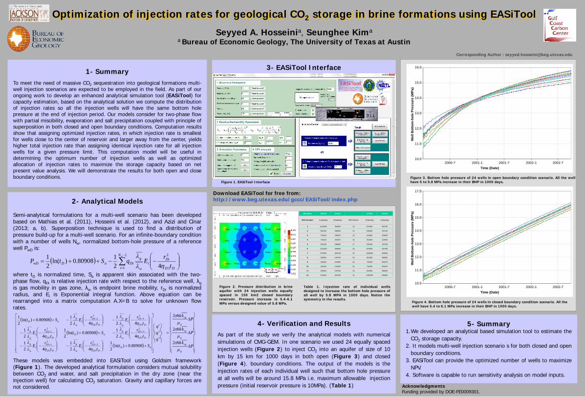
1- SummaryTo meet the need of massive CO2 sequestration into geological formations multi-well injection scenarios are expected to be employed in the field. As part of ourongoing work to develop an enhanced analytical simulation tool (EASiTool) forcapacity estimation, based on the analytical solution we compute the distributionof injection rates so all the injection wells will have the same bottom holepressure at the end of injection period. Our models consider for two-phase flowwith partial miscibility, evaporation and salt precipitation coupled with principle ofsuperposition in both closed and open boundary conditions. Computation resultsshow that assigning optimized injection rates, in which injection rate is smallestfor wells close to the center of reservoir and larger away from the center, yieldshigher total injection rate than assigning identical injection rate for all injectionwells for a given pressure limit. This computation model will be useful indetermining the optimum number of injection wells as well as optimizedallocation of injection rates to maximize the storage capacity based on netpresent value analysis. We will demonstrate the results for both open and closeboundary conditions.

Optimization of injection rates for geological CO2 storage in brine formations using EASiTool

Seyyed A. Hosseinia, Seunghee Kima

a Bureau of Economic Geology, The University of Texas at Austin

4- Verification and ResultsAs part of the study we verify the analytical models with numericalsimulations of CMG-GEM. In one scenario we used 24 equally spacedinjection wells (Figure 2) to inject CO2 into an aquifer of size of 10km by 15 km for 1000 days in both open (Figure 3) and closed(Figure 4). boundary conditions. The output of the models is theinjection rates of each individual well such that bottom hole pressureat all wells will be around 15.8 MPa i.e. maximum allowable injectionpressure (initial reservoir pressure is 10MPa). (Table 1)

Corresponding Author : seyyed.hosseini@beg.utexas.edu

2- Analytical Models

Semi-analytical formulations for a multi-well scenario has been developedbased on Mathias et al. (2011), Hosseini et al. (2012), and Azizi and Cinar(2013; a, b). Superposition technique is used to find a distribution ofpressure build-up for a multi-well scenario. For an infinite-boundary conditionwith a number of wells Nw, normalized bottom-hole pressure of a referencewell PwD is:

where tD is normalized time, Sa is apparent skin associated with the two-phase flow, qDi is relative injection rate with respect to the reference well, λgis gas mobility in gas zone, λw is endpoint brine mobility, rDi is normalizedradius, and Ei is Exponential integral function. Above equation can berearranged into a matrix computation A.X=B to solve for unknown flowrates.

These models was embedded into EASiTool using Goldsim framework(Figure 1). The developed analytical formulation considers mutual solubilitybetween CO2 and water, and salt precipitation in the dry zone (near theinjection well) for calculating CO2 saturation. Gravity and capillary forces arenot considered.

Figure 3. Bottom hole pressure of 24 wells in open boundary condition scenario. All the wellhave 5 to 5.8 MPa increase in their BHP in 1000 days.

3- EASiTool Interface

5- Summary1.We developed an analytical based simulation tool to estimate the

CO2 storage capacity.2. It models multi-well injection scenario s for both closed and open

boundary conditions.3. EASiTool can provide the optimized number of wells to maximize

NPV.4. Software is capable to run sensitivity analysis on model inputs.

Figure 4. Bottom hole pressure of 24 wells in closed boundary condition scenario. All thewell have 5.4 to 6.1 MPa increase in their BHP in 1000 days.

AcknowledgmentsFunding provided by DOE-FE0009301.

1

1 3

2

42180908.0)ln(

21 wN

i DD

Dii

w

gDiaDwD t

rEqStP

3

2

1

3

223

3

213

3

232

3

212

3

231

3

221

80908.0)ln(21

421

421

42180908.0)ln(

21

421

421

42180908.0)ln(

21

qqq

Stt

rEt

rE

trESt

trE

trE

trESt

aDDD

Di

w

g

DD

Di

w

g

DD

Di

w

gaD

DD

Di

w

g

DD

Di

w

g

DD

Di

w

gaD

Pkhk

Pkhk

Pkhk

g

rg

g

rg

g

rg

2

2

2

Boundary Infinite Closed Infinite Closed

Well Number Q [kg/day] Q [kg/day] Well Number Q [kg/day] Q [kg/day]

1 1152200 394650 13 874040 302790

2 831000 288000 14 528180 187240

3 734160 255070 15 431650 154050

4 734160 255070 16 431650 154050

5 831000 288000 17 528180 187240

6 1152200 394650 18 874040 302790

7 874040 302790 19 1152200 394650

8 528180 187240 20 831000 288000

9 431650 154050 21 734160 255070

10 431650 154050 22 734160 255070

11 528180 187240 23 831000 288000

12 874040 302790 24 1152200 394650

Table 1. Injection rate of individual wellsdesigned to increase the bottom hole pressure ofall well by 5.8 MPA in 1000 days. Notice thesymmetry in the results.

Figure 2. Pressure distribution in brineaquifer with 24 injection wells equallyspaced in 150 km2 closed boundaryreservoir. Pressure increase is 5.4-6.1MPa versus designed value of 5.8 MPa.

Figure 1. EASiTool Interface

Time (Date)

Wel

l Bot

tom

-hol

e Pr

essu

re (M

Pa)

2000-7 2001-1 2001-7 2002-1 2002-710.0

11.0

12.0

13.0

14.0

15.0

16.0

Time (Date)

Wel

l Bot

tom

-hol

e Pr

essu

re (M

Pa)

2000-7 2001-1 2001-7 2002-1 2002-710.0

11.0

12.0

13.0

14.0

15.0

16.0

17.0Download EASiTool for free from: http://www.beg.utexas.edu/gccc/EASiTool/index.php