Optimization of composite structures with curved fiber ...orbi.ulg.ac.be/bitstream/2268/184675/1/Bruyneel_B21.pdf · Optimization of composite structures with curved fiber trajectories

Composite Structures, 131, pp. 895-904, 2015.

1

Optimization of composite structures withcurved fiber trajectories

Etienne Lemaire1, Samih Zein1 and Michael Bruyneel1,2*

1SAMTECH s.a. (A Siemens Company), Liège Science Park,

Rue des Chasseurs-ardennais 8, Angleur, B-4031, Belgium2Aerospace & Mechanical Engineering Department, University of Liège, Belgium

* [email protected]

AbstractThis paper presents a new approach to generate and optimize parallel fibertrajectories on general non planar surfaces based on level-sets and the FastMarching Method. Starting with a (possibly curved) reference fiber directiondefined on a (possibly curved) meshed surface, the new method allows defining alevel-set representation of the fiber network for each ply, and so defining the fibertrajectories. This new approach is then used to solve optimization problems, inwhich the stiffness of the structure is maximized (minimum compliance problem).The design variables are the parameters defining the position and the shape of thereference curve. The shape of the design space is discussed, regarding local andglobal optimal solutions. The possibility to include in the optimization problem alimitation on the curvature of the trajectories is also addressed.

Keywords: optimization, fiber placement, level-set

1. IntroductionThe use of composite materials in aerospace, automotive and ship industry allowsmanufacturing lighter and more efficient mechanical structures. Indeed, properuse of the orthotropic properties of these materials enables further tailoring of thestructure to the loadings than when using isotropic materials. However, this comesat the cost of a more complicated design and sizing process firstly because of theorthotropic behavior of composite materials but also because of the manufacturingprocess which induces specific constraints in the use of these materials.From the mechanical point of view, one of the most important restrictionsresulting from the practical manufacturing of mechanical parts is the orientationof the reinforcement fibers resulting from the layup process. These orientationsdirectly determine the orthotropy axes and cannot be chosen arbitrarily in anypoint of a given part but rather result from the draping of the reinforcementmaterial over the part. Several models have been developed in order to predict theorientations of the reinforcement fibers after the draping process depending on theproperties of the reinforcement materials (see [1] for a review).

* Corresponding author: [email protected]


2

One of the first of these models is due to Mack and Taylor [2]. Often called the‘pin-jointed’ model [3], it is based on a geometric model of the woven and it iswell suited to predict the fiber orientation resulting from hand layup of dry wovenfabrics. Later, more complex models relying on a finite element mechanicalmodeling of the reinforcement have been developed for the forming ofpreimpregnated fabrics as for instance by Cherouat and Bourouchaki [4].

Besides the manufacturing of composites part by hand layup of large pieces ofreinforcement material, another group of methods is gaining interest since its firstintroduction in the 1970s. These methods rely on the robotized layup of bands ofunidirectional reinforcement material allowing more accurate and more repeatablemanufacturing process [5]. In this group, two main methods can be identifiedAutomated Tape Layup (ATL) and Automated Fiber Placement (AFP). ATLmakes use of a robotic arm to layup tapes (up to 300mm wide) of unidirectionalprepeg and benefits from high productivity for large and simple flat parts. ButATL main limitation comes from the relatively high minimum curvature radius(up to 6m) that can be applied to the prepreg tape without wrinkling. With AFP,this minimum curvature radius is decreased to 50cm by subdividing the tape intoseveral tows which can be cut and restarted individually. Therefore themanufacturing of more complicated parts can be handled by AFP but with a lowerproductivity than ATL.

For ATL and AFP processes, one of the manufacturing issues is the determinationof successive courses trajectories. Indeed, for these processes, it is crucial thatthere are no overlaps and no gaps between adjacent courses in order to ensuremaximal strength and minimum weight for the final part. In other words, thismeans that successive layup courses have to be equidistant.

A few researchers have studied the optimal design of ATL/AFP parts. A firstgroup of methods consists in defining an initial course which is then simplyshifted over the part to define subsequent course as proposed by Tatting andGürdal [6, 7]. Secondly, the courses can be defined as geodesic paths, constantangle paths, linearly varying angle paths or constant curvature path [8]. However,these two approaches do not result in equidistant paths. Alternatively, thesubsequent courses can be obtained by computing actual offset curves from aninitial curve. This approach is more difficult but leads to equidistant courses andhas been investigated by Waldhart [9], Shirinzadeh et al [10] and Bruyneel andZein [11] with different numerical schemes. The two first groups of authorspropose an approach based on a geometrical description of the part while the thirdone developed an algorithm able to work with a level-set representation on a meshof the layup surface. In [12], Bruyneel and Zein used their approach in aparametric study in order to determine the effect on the structural stiffness ofcurving the fiber trajectory of a single ply laid on a cantilever structure (see also[13]). It is also worth mentioning the work done recently by Brampton and Kim[14] where level-set and optimization approaches are used on planar structures.

The goal of the present paper is to demonstrate further the capabilities of themethod proposed by Bruyneel and Zein [11], which is available in an industrialcontext, by using it for optimal design of composite parts.


3

This paper starts with a brief introduction describing the method developed in[11,12] to determine equidistant courses for ATL/AFP process. Next, severaloptimization problems with growing complexity are studied in order to illustratethe interest of the method.

2. Fiber placement modeling

2.1 Fast Marching Method

Bruyneel and Zein [11,12] first proposed the use of level-set and Fast MarchingMethod (FMM, see [15]) to solve the problem of determining equidistant courseson an arbitrary layup surface. The Fast Marching Method aims at solving theEikonal equation:

(1)

The problem given in Eq. (1) consists in finding a scalar field such that the

norm of its gradient is constant over the domain and that the value of is equal

to zero on a curve of .

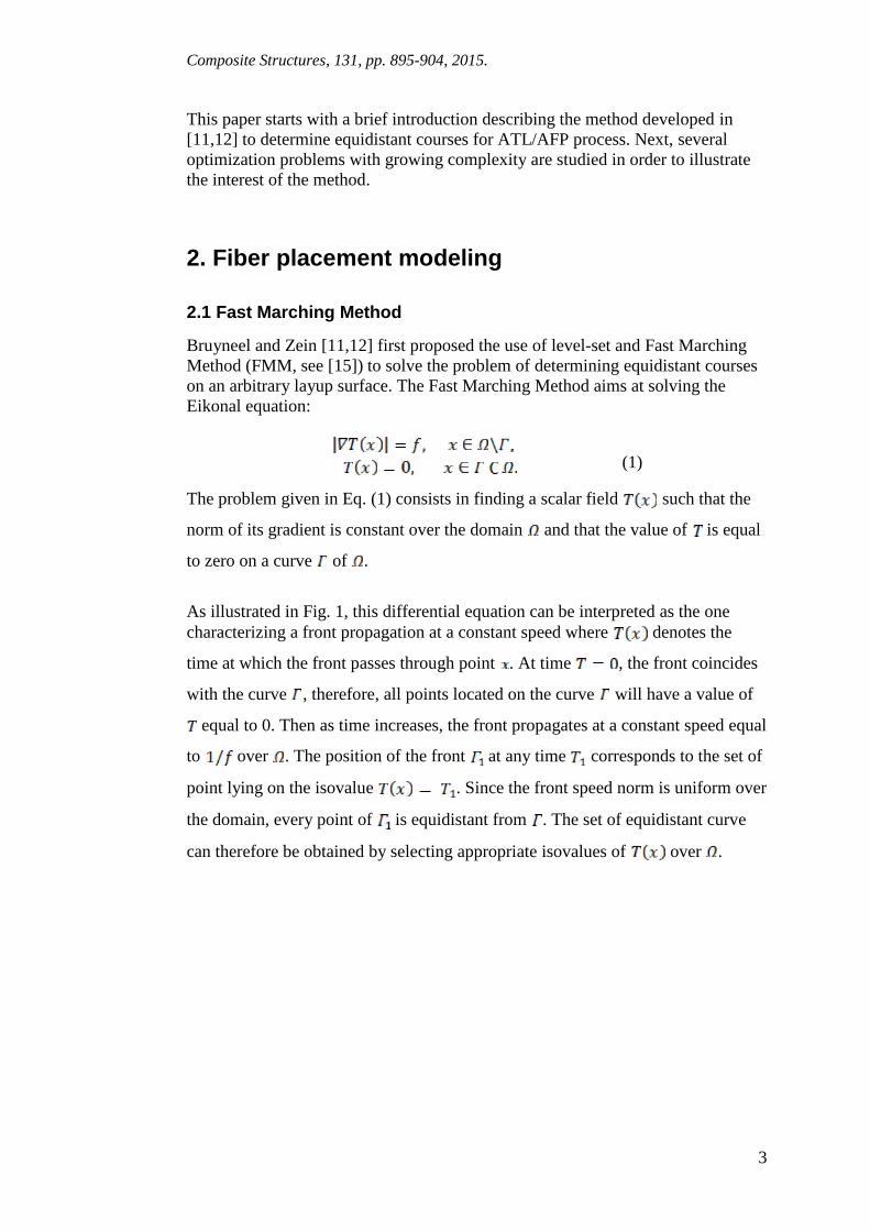
As illustrated in Fig. 1, this differential equation can be interpreted as the onecharacterizing a front propagation at a constant speed where denotes the

time at which the front passes through point . At time , the front coincides

with the curve , therefore, all points located on the curve will have a value of

equal to 0. Then as time increases, the front propagates at a constant speed equal

to over . The position of the front at any time corresponds to the set of

point lying on the isovalue . Since the front speed norm is uniform over

the domain, every point of is equidistant from . The set of equidistant curve

can therefore be obtained by selecting appropriate isovalues of over .


4

Figure 1. Front propagation interpretation of Eikonal equation.

Based on a triangular mesh of the layup surface, the developed procedure allowscomputing fiber orientation on each element of the mesh. At first one needs todefine the initial front position on the layup surface. This curve corresponds to thereference course and the definition procedure is presented in next subsection.Secondly, the Fast Marching Method is used to solve the Eikonal equation and tocompute the time T at any point of the mesh. The function T(x) is supposed to bepiecewise linear by element. Starting from initial values defined by the referencecurve, the value of T is progressively computed on the domain by solving theEikonal equation locally on each triangle of the mesh. For further details about theFast Marching Method, the interested reader may refer to [15]. Finally, the fiberorientations on each element are defined by computing the direction of theisovalues of T(x) over the considered element. Since those isovalues areequidistant from the reference course, the computed orientations correspond to agap-less and overlap-less (i.e. constant thickness) layup obtained by ATL or AFP.

2.2 Reference course tracing

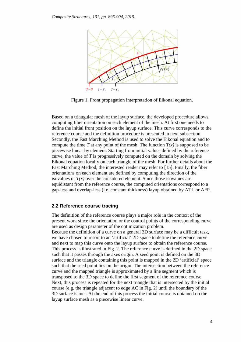
The definition of the reference course plays a major role in the context of thepresent work since the orientation or the control points of the corresponding curveare used as design parameter of the optimization problem.Because the definition of a curve on a general 3D surface may be a difficult task,we have chosen to resort to an ‘artificial’ 2D space to define the reference curveand next to map this curve onto the layup surface to obtain the reference course.This process is illustrated in Fig. 2. The reference curve is defined in the 2D spacesuch that it passes through the axes origin. A seed point is defined on the 3Dsurface and the triangle containing this point is mapped in the 2D ‘artificial’ spacesuch that the seed point lies on the origin. The intersection between the referencecurve and the mapped triangle is approximated by a line segment which istransposed to the 3D space to define the first segment of the reference course.Next, this process is repeated for the next triangle that is intersected by the initialcourse (e.g. the triangle adjacent to edge AC in Fig. 2) until the boundary of the3D surface is met. At the end of this process the initial course is obtained on thelayup surface mesh as a piecewise linear curve.


5

Figure 2. Reference course mapping.

3. Straight course optimization

3.1 Optimization problem

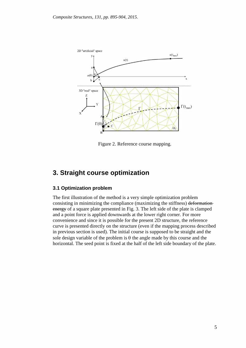
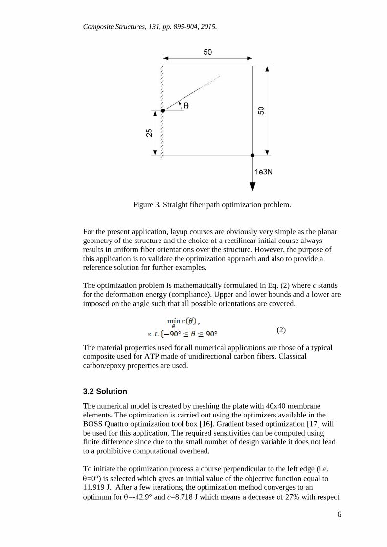
The first illustration of the method is a very simple optimization problemconsisting in minimizing the compliance (maximizing the stiffness) deformationenergy of a square plate presented in Fig. 3. The left side of the plate is clampedand a point force is applied downwards at the lower right corner. For moreconvenience and since it is possible for the present 2D structure, the referencecurve is presented directly on the structure (even if the mapping process describedin previous section is used). The initial course is supposed to be straight and thesole design variable of the problem is the angle made by this course and thehorizontal. The seed point is fixed at the half of the left side boundary of the plate.


6

Figure 3. Straight fiber path optimization problem.

For the present application, layup courses are obviously very simple as the planargeometry of the structure and the choice of a rectilinear initial course alwaysresults in uniform fiber orientations over the structure. However, the purpose ofthis application is to validate the optimization approach and also to provide areference solution for further examples.

The optimization problem is mathematically formulated in Eq. (2) where c standsfor the deformation energy (compliance). Upper and lower bounds and a lower areimposed on the angle such that all possible orientations are covered.

(2)

The material properties used for all numerical applications are those of a typicalcomposite used for ATP made of unidirectional carbon fibers. Classicalcarbon/epoxy properties are used.

3.2 Solution

The numerical model is created by meshing the plate with 40x40 membraneelements. The optimization is carried out using the optimizers available in theBOSS Quattro optimization tool box [16]. Gradient based optimization [17] willbe used for this application. The required sensitivities can be computed usingfinite difference since due to the small number of design variable it does not leadto a prohibitive computational overhead.

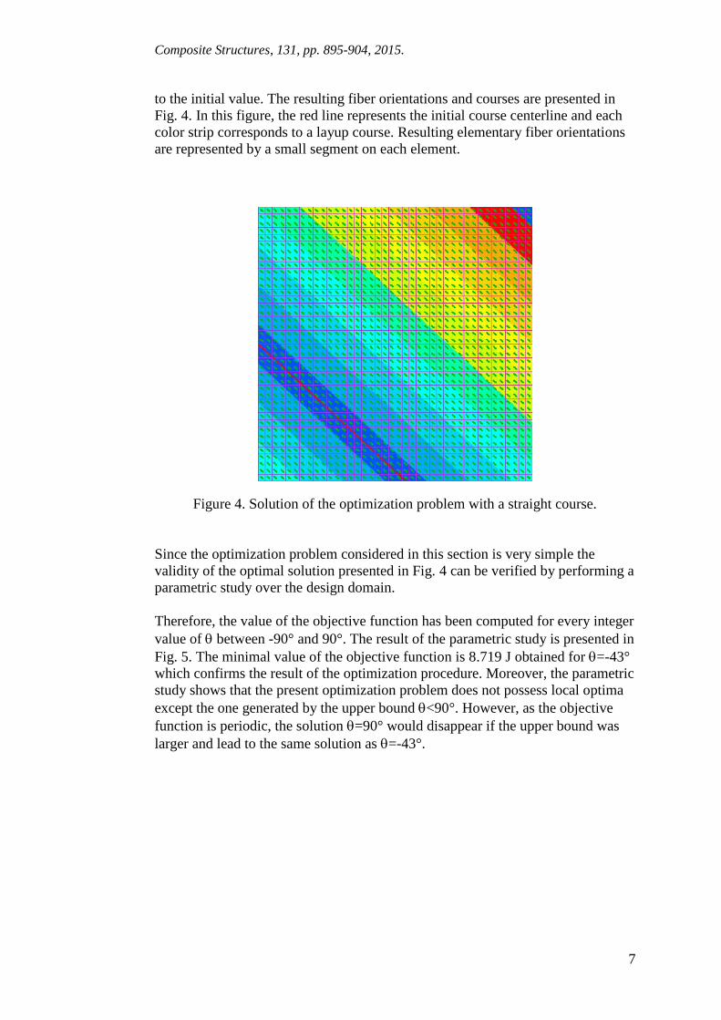
To initiate the optimization process a course perpendicular to the left edge (i.e.=0°) is selected which gives an initial value of the objective function equal to11.919 J. After a few iterations, the optimization method converges to anoptimum for =-42.9° and c=8.718 J which means a decrease of 27% with respect


7

to the initial value. The resulting fiber orientations and courses are presented inFig. 4. In this figure, the red line represents the initial course centerline and eachcolor strip corresponds to a layup course. Resulting elementary fiber orientationsare represented by a small segment on each element.

Figure 4. Solution of the optimization problem with a straight course.

Since the optimization problem considered in this section is very simple thevalidity of the optimal solution presented in Fig. 4 can be verified by performing aparametric study over the design domain.

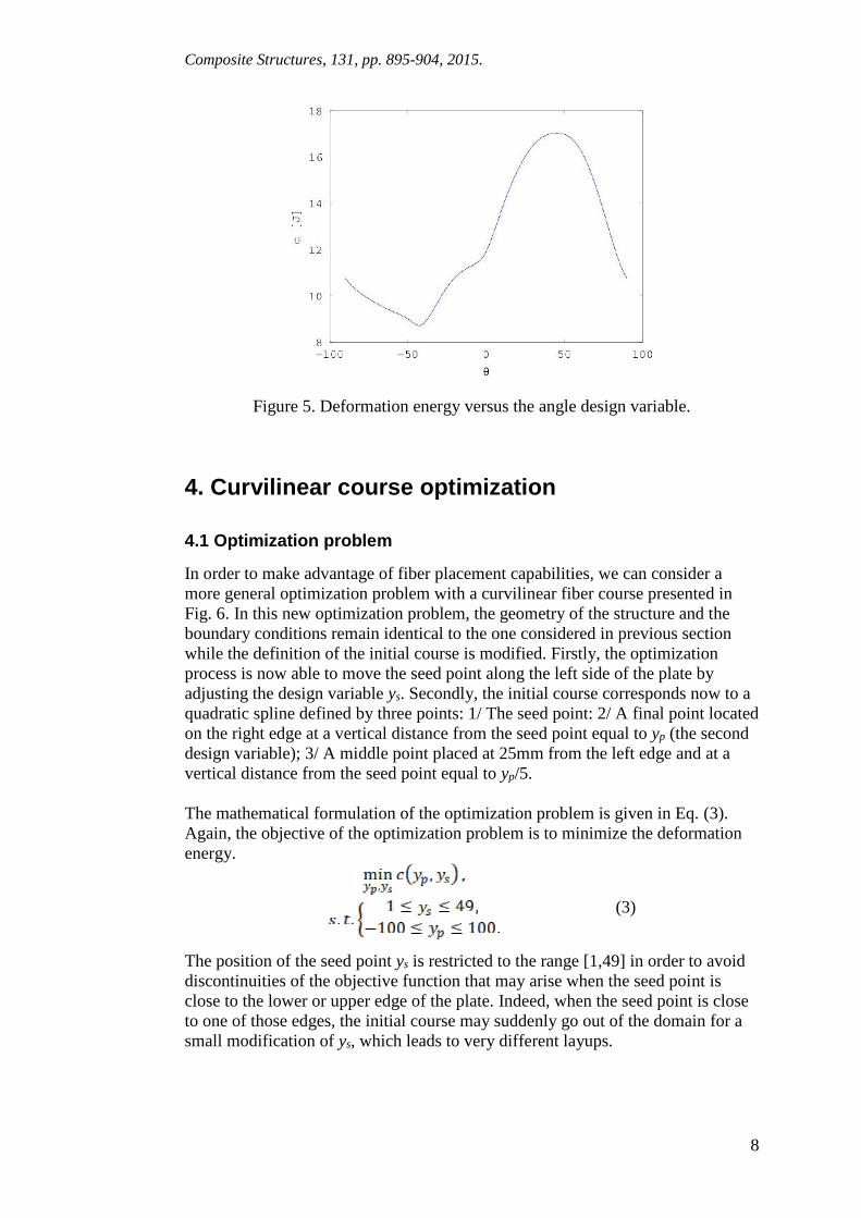
Therefore, the value of the objective function has been computed for every integervalue of between -90° and 90°. The result of the parametric study is presented inFig. 5. The minimal value of the objective function is 8.719 J obtained for =-43°which confirms the result of the optimization procedure. Moreover, the parametricstudy shows that the present optimization problem does not possess local optimaexcept the one generated by the upper bound <90°. However, as the objectivefunction is periodic, the solution =90° would disappear if the upper bound waslarger and lead to the same solution as =-43°.


8

Figure 5. Deformation energy versus the angle design variable.

4. Curvilinear course optimization


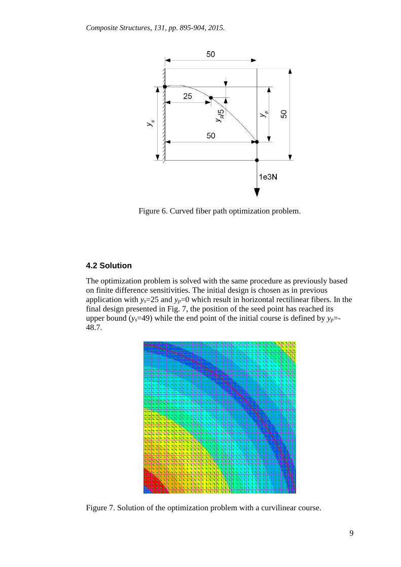
In order to make advantage of fiber placement capabilities, we can consider amore general optimization problem with a curvilinear fiber course presented inFig. 6. In this new optimization problem, the geometry of the structure and theboundary conditions remain identical to the one considered in previous sectionwhile the definition of the initial course is modified. Firstly, the optimizationprocess is now able to move the seed point along the left side of the plate byadjusting the design variable ys. Secondly, the initial course corresponds now to aquadratic spline defined by three points: 1/ The seed point: 2/ A final point locatedon the right edge at a vertical distance from the seed point equal to yp (the seconddesign variable); 3/ A middle point placed at 25mm from the left edge and at avertical distance from the seed point equal to yp/5.

The mathematical formulation of the optimization problem is given in Eq. (3).Again, the objective of the optimization problem is to minimize the deformationenergy.

(3)

The position of the seed point ys is restricted to the range [1,49] in order to avoiddiscontinuities of the objective function that may arise when the seed point isclose to the lower or upper edge of the plate. Indeed, when the seed point is closeto one of those edges, the initial course may suddenly go out of the domain for asmall modification of ys, which leads to very different layups.


9

Figure 6. Curved fiber path optimization problem.

4.2 Solution

The optimization problem is solved with the same procedure as previously basedon finite difference sensitivities. The initial design is chosen as in previousapplication with ys=25 and yp=0 which result in horizontal rectilinear fibers. In thefinal design presented in Fig. 7, the position of the seed point has reached itsupper bound (ys=49) while the end point of the initial course is defined by yp=-48.7.

Figure 7. Solution of the optimization problem with a curvilinear course.


10

Under the design load case, the final design gives a deformation energy which is61% less than the initial design and 46% less than the rectilinear design obtainedpreviously. This shows that the capability of AFP to follow curved courses leadsto a strong improvement of the mechanical performance and confirms theconclusions of Hyer and Charette [18]. Nevertheless, we can observe that thecurvature of the courses increases in the lower left corner such that theintroduction of an optimization constraint on curvature would be helpful to ensurethe manufacturability of the part. This issue will be addressed in Section 6.

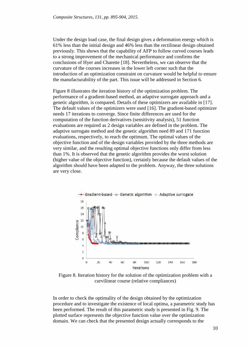
Figure 8 illustrates the iteration history of the optimization problem. Theperformance of a gradient-based method, an adaptive surrogate approach and agenetic algorithm, is compared. Details of these optimizers are available in [17].The default values of the optimizers were used [16]. The gradient-based optimizerneeds 17 iterations to converge. Since finite differences are used for thecomputation of the function derivatives (sensitivity analysis), 51 functionevaluations are required as 2 design variables are defined in the problem. Theadaptive surrogate method and the genetic algorithm need 89 and 171 functionevaluations, respectively, to reach the optimum. The optimal values of theobjective function and of the design variables provided by the three methods arevery similar, and the resulting optimal objective functions only differ from lessthan 1%. It is observed that the genetic algorithm provides the worst solution(higher value of the objective function), certainly because the default values of thealgorithm should have been adapted to the problem. Anyway, the three solutionsare very close.

Figure 8. Iteration history for the solution of the optimization problem with acurvilinear course (relative compliances)

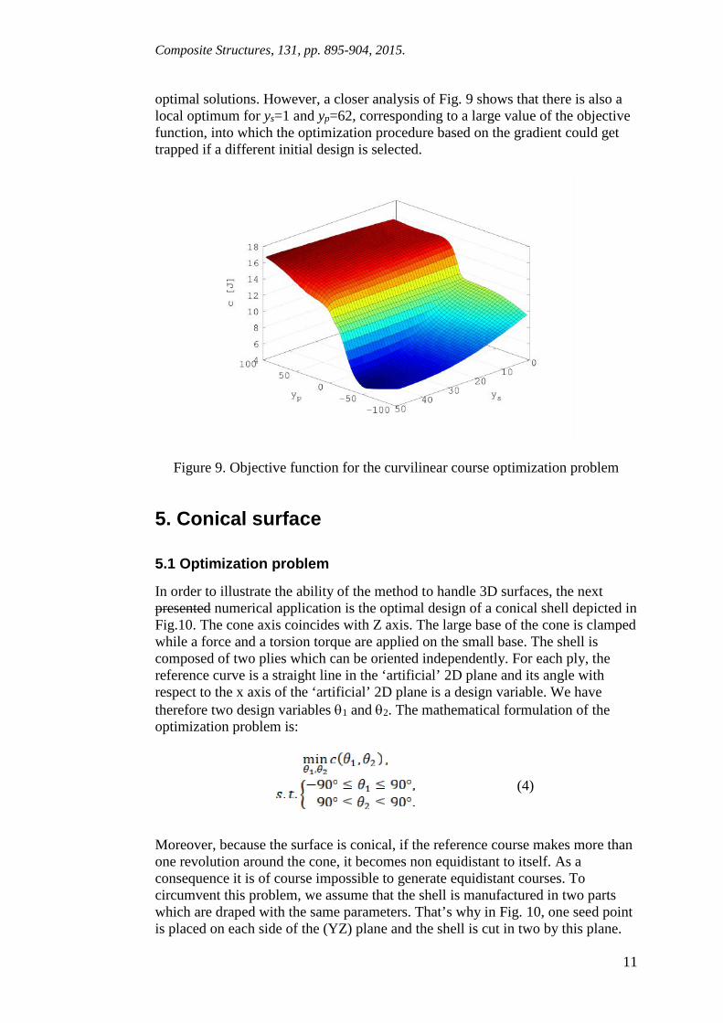
In order to check the optimality of the design obtained by the optimizationprocedure and to investigate the existence of local optima, a parametric study hasbeen performed. The result of this parametric study is presented in Fig. 9. Theplotted surface represents the objective function value over the optimizationdomain. We can check that the presented design actually corresponds to the


11

optimal solutions. However, a closer analysis of Fig. 9 shows that there is also alocal optimum for ys=1 and yp=62, corresponding to a large value of the objectivefunction, into which the optimization procedure based on the gradient could gettrapped if a different initial design is selected.

Figure 9. Objective function for the curvilinear course optimization problem

5. Conical surface


In order to illustrate the ability of the method to handle 3D surfaces, the nextpresented numerical application is the optimal design of a conical shell depicted inFig.10. The cone axis coincides with Z axis. The large base of the cone is clampedwhile a force and a torsion torque are applied on the small base. The shell iscomposed of two plies which can be oriented independently. For each ply, thereference curve is a straight line in the ‘artificial’ 2D plane and its angle withrespect to the x axis of the ‘artificial’ 2D plane is a design variable. We havetherefore two design variables 1 and 2. The mathematical formulation of theoptimization problem is:

(4)

Moreover, because the surface is conical, if the reference course makes more thanone revolution around the cone, it becomes non equidistant to itself. As aconsequence it is of course impossible to generate equidistant courses. Tocircumvent this problem, we assume that the shell is manufactured in two partswhich are draped with the same parameters. That’s why in Fig. 10, one seed pointis placed on each side of the (YZ) plane and the shell is cut in two by this plane.


12

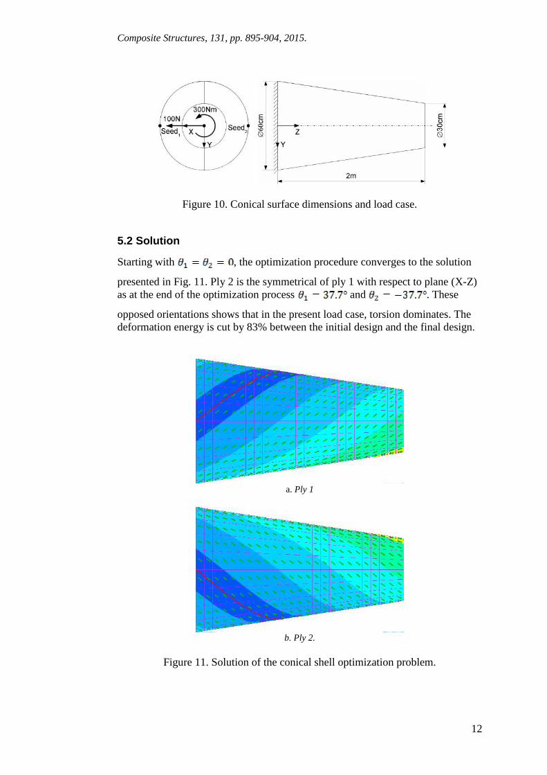
Figure 10. Conical surface dimensions and load case.

5.2 Solution

Starting with , the optimization procedure converges to the solution

presented in Fig. 11. Ply 2 is the symmetrical of ply 1 with respect to plane (X-Z)as at the end of the optimization process and . These

opposed orientations shows that in the present load case, torsion dominates. Thedeformation energy is cut by 83% between the initial design and the final design.

a. Ply 1

b. Ply 2.

Figure 11. Solution of the conical shell optimization problem.


13

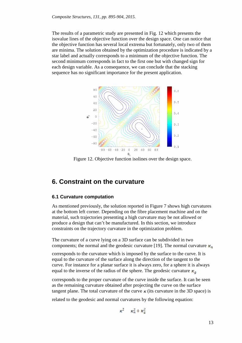
The results of a parametric study are presented in Fig. 12 which presents theisovalue lines of the objective function over the design space. One can notice thatthe objective function has several local extrema but fortunately, only two of themare minima. The solution obtained by the optimization procedure is indicated by astar label and actually corresponds to a minimum of the objective function. Thesecond minimum corresponds in fact to the first one but with changed sign foreach design variable. As a consequence, we can conclude that the stackingsequence has no significant importance for the present application.

Figure 12. Objective function isolines over the design space.

6. Constraint on the curvature

6.1 Curvature computation

As mentioned previously, the solution reported in Figure 7 shows high curvaturesat the bottom left corner. Depending on the fibre placement machine and on thematerial, such trajectories presenting a high curvature may be not allowed orproduce a design that can’t be manufactured. In this section, we introduceconstraints on the trajectory curvature in the optimization problem.

The curvature of a curve lying on a 3D surface can be subdivided in twocomponents; the normal and the geodesic curvature [19]. The normal curvature

corresponds to the curvature which is imposed by the surface to the curve. It isequal to the curvature of the surface along the direction of the tangent to thecurve. For instance for a planar surface it is always zero, for a sphere it is alwaysequal to the inverse of the radius of the sphere. The geodesic curvature

corresponds to the proper curvature of the curve inside the surface. It can be seenas the remaining curvature obtained after projecting the curve on the surfacetangent plane. The total curvature of the curve (its curvature in the 3D space) is

related to the geodesic and normal curvatures by the following equation:


14

From an ATP/AFP manufacturing point of view, the geodesic curvaturedetermines the in plane bending applied to the fiber tape or tow. This is thedirection in which the tapes and the tows are the less flexible and attempting toimpose a too low turning radius may lead to defects. This is why we focus here onevaluating the geodesic curvature of the fibers.

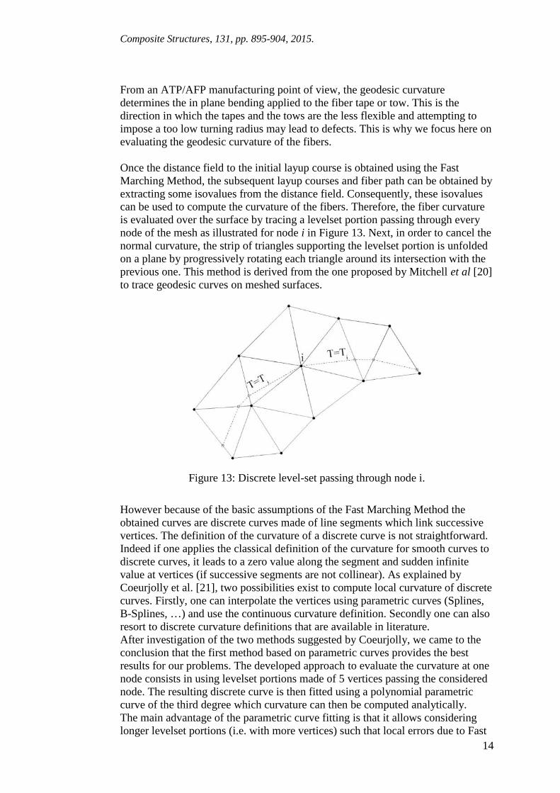
Once the distance field to the initial layup course is obtained using the FastMarching Method, the subsequent layup courses and fiber path can be obtained byextracting some isovalues from the distance field. Consequently, these isovaluescan be used to compute the curvature of the fibers. Therefore, the fiber curvatureis evaluated over the surface by tracing a levelset portion passing through everynode of the mesh as illustrated for node i in Figure 13. Next, in order to cancel thenormal curvature, the strip of triangles supporting the levelset portion is unfoldedon a plane by progressively rotating each triangle around its intersection with theprevious one. This method is derived from the one proposed by Mitchell et al [20]to trace geodesic curves on meshed surfaces.

Figure 13: Discrete level-set passing through node i.

However because of the basic assumptions of the Fast Marching Method theobtained curves are discrete curves made of line segments which link successivevertices. The definition of the curvature of a discrete curve is not straightforward.Indeed if one applies the classical definition of the curvature for smooth curves todiscrete curves, it leads to a zero value along the segment and sudden infinitevalue at vertices (if successive segments are not collinear). As explained byCoeurjolly et al. [21], two possibilities exist to compute local curvature of discretecurves. Firstly, one can interpolate the vertices using parametric curves (Splines,B-Splines, …) and use the continuous curvature definition. Secondly one can alsoresort to discrete curvature definitions that are available in literature.After investigation of the two methods suggested by Coeurjolly, we came to theconclusion that the first method based on parametric curves provides the bestresults for our problems. The developed approach to evaluate the curvature at onenode consists in using levelset portions made of 5 vertices passing the considerednode. The resulting discrete curve is then fitted using a polynomial parametriccurve of the third degree which curvature can then be computed analytically.The main advantage of the parametric curve fitting is that it allows consideringlonger levelset portions (i.e. with more vertices) such that local errors due to Fast


15

Marching Approximation are more efficiently smoothed out than when resortingto discrete curvature definition which only allows considering levelset portionsmade of three vertices. The method has been tested on a spherical benchmark forwhich geodesic curvature can be computed analytically and shows to generallyprovide a very good estimation of geodesic curvature excepted on the boundary ofthe surface due to the fact that it is not possible to trace a levelset portion on bothside of the considered nodes. For this reason, we decided to discard the boundarynodes from the curvature computation. Indeed, as we will see in the results, evenif the maximum curvature values usually appear close to the boundary, thecurvature distribution is sufficiently smooth to avoid a too large error.

6.2 Illustration

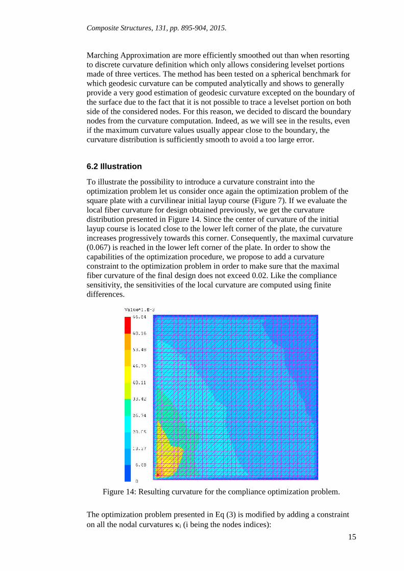
To illustrate the possibility to introduce a curvature constraint into theoptimization problem let us consider once again the optimization problem of thesquare plate with a curvilinear initial layup course (Figure 7). If we evaluate thelocal fiber curvature for design obtained previously, we get the curvaturedistribution presented in Figure 14. Since the center of curvature of the initiallayup course is located close to the lower left corner of the plate, the curvatureincreases progressively towards this corner. Consequently, the maximal curvature(0.067) is reached in the lower left corner of the plate. In order to show thecapabilities of the optimization procedure, we propose to add a curvatureconstraint to the optimization problem in order to make sure that the maximalfiber curvature of the final design does not exceed 0.02. Like the compliancesensitivity, the sensitivities of the local curvature are computed using finitedifferences.

Figure 14: Resulting curvature for the compliance optimization problem.

The optimization problem presented in Eq (3) is modified by adding a constrainton all the nodal curvatures i (i being the nodes indices):


16

(5)

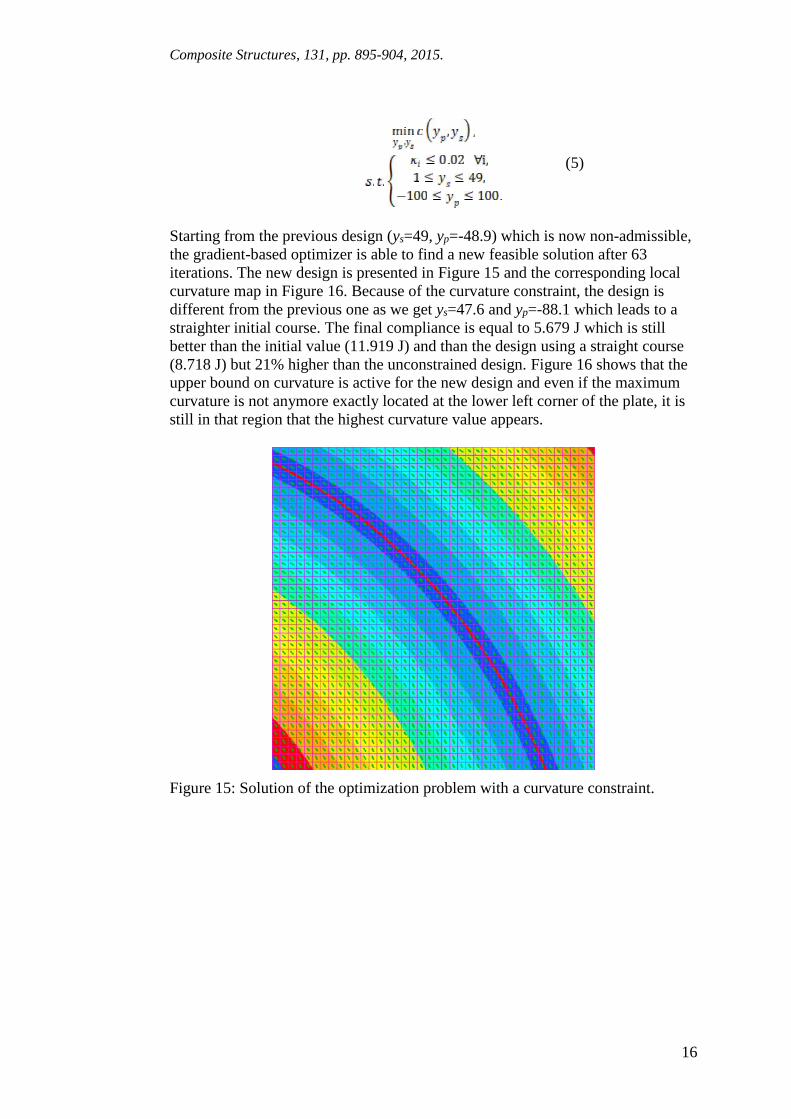
Starting from the previous design (ys=49, yp=-48.9) which is now non-admissible,the gradient-based optimizer is able to find a new feasible solution after 63iterations. The new design is presented in Figure 15 and the corresponding localcurvature map in Figure 16. Because of the curvature constraint, the design isdifferent from the previous one as we get ys=47.6 and yp=-88.1 which leads to astraighter initial course. The final compliance is equal to 5.679 J which is stillbetter than the initial value (11.919 J) and than the design using a straight course(8.718 J) but 21% higher than the unconstrained design. Figure 16 shows that theupper bound on curvature is active for the new design and even if the maximumcurvature is not anymore exactly located at the lower left corner of the plate, it isstill in that region that the highest curvature value appears.

Figure 15: Solution of the optimization problem with a curvature constraint.


17

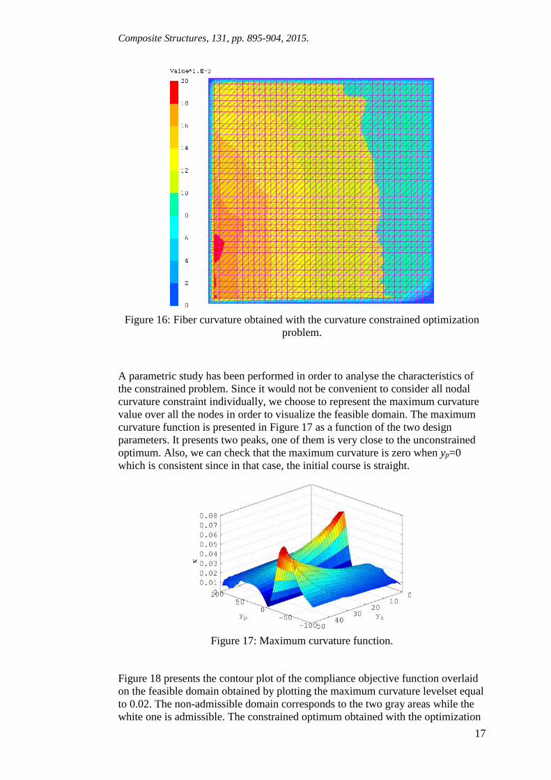
Figure 16: Fiber curvature obtained with the curvature constrained optimizationproblem.

A parametric study has been performed in order to analyse the characteristics ofthe constrained problem. Since it would not be convenient to consider all nodalcurvature constraint individually, we choose to represent the maximum curvaturevalue over all the nodes in order to visualize the feasible domain. The maximumcurvature function is presented in Figure 17 as a function of the two designparameters. It presents two peaks, one of them is very close to the unconstrainedoptimum. Also, we can check that the maximum curvature is zero when yp=0which is consistent since in that case, the initial course is straight.

Figure 17: Maximum curvature function.

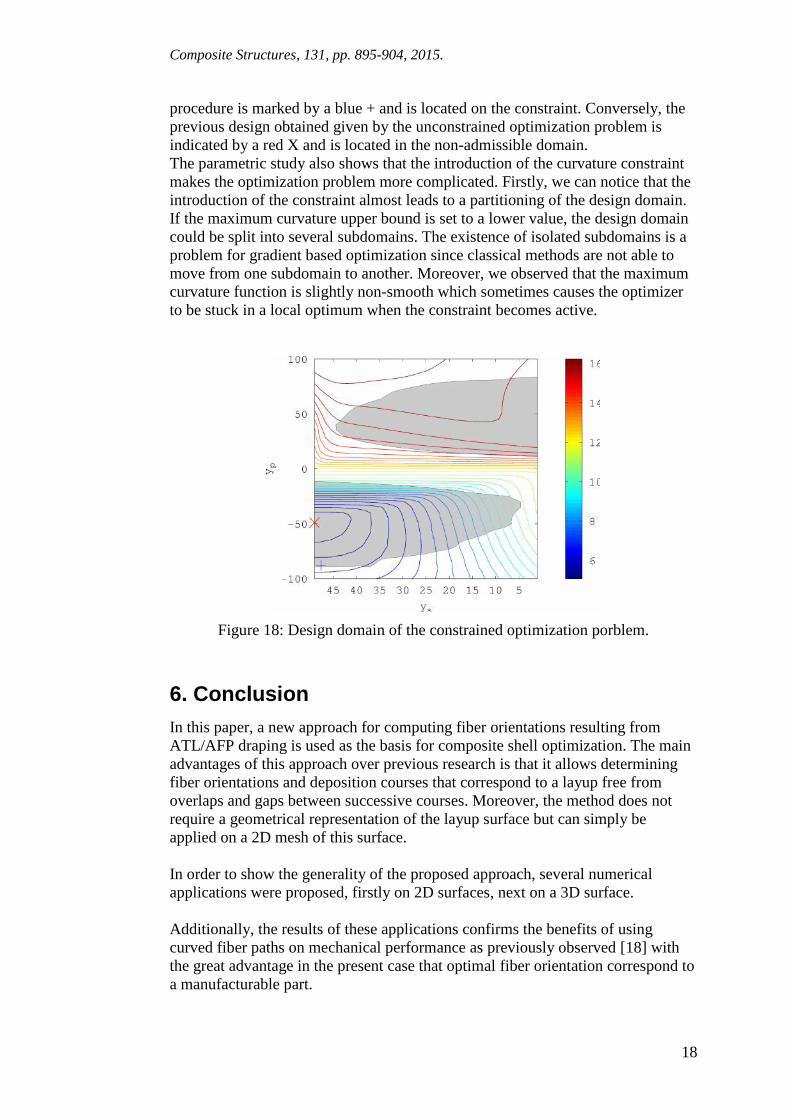
Figure 18 presents the contour plot of the compliance objective function overlaidon the feasible domain obtained by plotting the maximum curvature levelset equalto 0.02. The non-admissible domain corresponds to the two gray areas while thewhite one is admissible. The constrained optimum obtained with the optimization


18

procedure is marked by a blue + and is located on the constraint. Conversely, theprevious design obtained given by the unconstrained optimization problem isindicated by a red X and is located in the non-admissible domain.The parametric study also shows that the introduction of the curvature constraintmakes the optimization problem more complicated. Firstly, we can notice that theintroduction of the constraint almost leads to a partitioning of the design domain.If the maximum curvature upper bound is set to a lower value, the design domaincould be split into several subdomains. The existence of isolated subdomains is aproblem for gradient based optimization since classical methods are not able tomove from one subdomain to another. Moreover, we observed that the maximumcurvature function is slightly non-smooth which sometimes causes the optimizerto be stuck in a local optimum when the constraint becomes active.

Figure 18: Design domain of the constrained optimization porblem.

6. ConclusionIn this paper, a new approach for computing fiber orientations resulting fromATL/AFP draping is used as the basis for composite shell optimization. The mainadvantages of this approach over previous research is that it allows determiningfiber orientations and deposition courses that correspond to a layup free fromoverlaps and gaps between successive courses. Moreover, the method does notrequire a geometrical representation of the layup surface but can simply beapplied on a 2D mesh of this surface.

In order to show the generality of the proposed approach, several numericalapplications were proposed, firstly on 2D surfaces, next on a 3D surface.

Additionally, the results of these applications confirms the benefits of usingcurved fiber paths on mechanical performance as previously observed [18] withthe great advantage in the present case that optimal fiber orientation correspond toa manufacturable part.


19

Finally, a constraint on a minimum curvature radius for the layup courses wasdefined and introduced in the optimization problem.

As developed in commercial pieces of software, the solution is available forindustrial applications. However, future work should, for instance, focus on theimprovement of the sensitivity analysis. The development of a semi-analyticalsensitivity analysis would strongly improve the efficiency of the optimizationprocess and would allow increasing the number of design variables in order toconsider more complex courses definition.

AcknowledgementPart of this work was supported by Wallonia (Belgium), in the DRAPOPT project.

References1. T.-C. Lim and S. Ramakrishna, "Modelling of composite sheet forming: A review," Composites - Part

A: Applied Science and Manufacturing, vol. 33, no. 4, pp. 515-537, 2002.2. C. Mack and H. Taylor, "The fitting of woven cloth to surfaces," Journal of the Textile Institute, vol.

47, pp. 477-488, 1956.3. F. Van Der Weeën, "Algorithms for draping fabrics on doubly-curved surfaces," International Journal

for Numerical Methods in Engineering, vol. 31, no. 7, pp. 1415-1426, 1991.4. A. Cherouat and H. Bourouchaki, "Numerical tools for composite woven fabric preforming," Advances

in Materials Science and Engineering, vol. 2013, 2013.5. D.-J. Lukaszewicz, C. Ward and K. Potter, "The engineering aspects of automated prepreg layup:

History, present and future," Composites Part B: Engineering, vol. 43, pp. 997-1009, 2012.6. B. Tatting and Z. Gürdal, "Design and manufacure of elastically tailored tow placed plates,"

NASA/CR--2002-211919, 2002.7. Z. Gürdal, B. Tatting and C. Wu, "Variable stiffness composite panels: Effects of stiffness variation on

the in-plane and buckling response," Composites Part A: Applied Science and Manufacturing, vol. 39, no. 5,pp. 911-922, 2008.

8. A. Blom, B. Tatting, J. Hol and Z. Gürdal, "Fiber path definitions for elastically tailored conicalshells," Composites Part B: Engineering, vol. 40, no. 1, pp. 77-84, 2009.

9. C. Waldhart, "Analysis of Tow-Placed, Variable-Stiffness Laminates," 1996.10. B. Shirinzadeh, G. Cassidy, D. Oetomo, G. Alici and M. Ang, "Trajectory generation for open-

contoured structures in robotic fibre placement," Robotics and Computer-Integrated Manufacturing, vol. 23,pp. 380-394, 2007.

11. M. Bruyneel and S. Zein, "A modified Fast Marching Method for defining fiber placement trajectoriesover meshes," Computers and Structures, vol. 125, pp. 45-52, 2013.

12. M. Bruyneel and S. Zein. "A new strategy avoiding gaps and overlaps in the simulation of fiberplacement trajectories", International Conference on Composite Structures – ICCS16, June 28-30, 2011,Porto, Portugal.

13. M. Bruyneel, J.C. Craveur, P. Gourmelen. "Optimisation des structures mécaniques: methodesnumériques et éléments finis", Dunod, Paris, 2014.

14. C.J. Brampton and H.A. Kim. "Optimization of tow steerd fiber orientation using the level setmethod”, 10th World Congress on Structural and Multidisciplinary Optimization, May 19-24, 2013, Orlando,Florida, USA.

15. J. Sethian, Level Set Methods and Fast Marching Methods, Cambridge University Press, 1999.16. Y. Radovcic and A. Remouchamps, "BOSS QUATTRO: an open system for parametric design,"

Structural and Multidisciplinary Optimization, vol. 23, no. 2, pp. 140-152, 2002.17. B. Colson, M. Bruyneel, S. Grihon, C. Raick and A. Remouchamps, "Colson B., Bruyneel M., Grihon

S., Raick C. and Remouchamps A. (2010). "Optimisation methods for advanced design of aircraft panels: acomparison", Optimisation & Engineering, 11(4), pp. 583-596.

18. M. Hyer and R. Charette, "Use of curvilinear fiber format in composite structure design," AIAAJournal, vol. 29, no. 6, pp. 1011-1015, 1991.

19. A. Pressley. Elementary differential geometry, London, Springer-Verlag, 2012.20. J. Mitchell, D. Mount and C. Papadimitriou. "The discrete geodesic problem", SIAM Journal of

Computing, 16 (4), pp. 647-668, 1987.21. D. Coeurjolly, S. Miguet and L. Tougne. "Discrete curvature based on osculating circle estimation",

in Visual Form 2001, Lecture Notes in Computer Science, vol. 2059, pp. 303-312, 2001.

Documents

Optimization of composite structures with curved fiber ...orbi.ulg.ac.be/bitstream/2268/184675/1/Bruyneel_B21.pdf · Optimization of composite structures with curved fiber trajectories