Compressive Response of Tapered Curved Composite … · Compressive Response of Tapered Curved Composite Plates ... Compressive Response of Tapered Curved Composite Plates ... I would

Compressive Response of Tapered Curved Composite Plates

Shaikh Mohammed Akhlaque-E-Rasul

A Thesis

in

The Department

of

Mechanical and Industrial Engineering

Presented in Partial Fulfillment of the Requirements

for the Degree of Doctor of Philosophy at

Concordia University

Montreal, Quebec, Canada

December 2010

© Shaikh Akhlaque, 2010

Shaikh Mohammed Akhlaque-E-rasul


Dr. Nawwaf Kharma, Dept. of Elect. & Comp. Eng.

Dr. Ronald Gibson, Dept. of Mech. Eng., U. of Nevada-Reno

Dr. M. Soleymani, Dept. of Elect. & Comp. Eng.

Dr. S. V. Hoa

Dr. M. Medraj

Dr. R. Ganesan

iii

ABSTRACT


Shaikh Mohammed Akhlaque-E-Rasul, Ph.D.

Concordia University, 2010

Tapered laminated structures have considerable potential for creating significant weight

savings in engineering applications. In the present thesis, the ply failure and global

buckling failure of internally-tapered curved laminates are considered. For the buckling

analysis, four different analytical approaches are employed: (1) classical shell theories

using Ritz method, (2) first-order shear deformation shell theories using Ritz method, (3)

linear finite element analysis based on first-order shear deformation shell theories, and

(4) non-linear finite element analysis. Due to the variety of tapered curved composite

plates and the complexity of the analysis, no closed-form analytical solution is available

at present regarding their response to compressive loading. Therefore, the Ritz method is

used for the global buckling analysis considering uniaxial compressive load. Linear

buckling analysis of the plates is carried out based on eight classical shell theories and six

first-order shear deformation shell theories. To apply the first-order shear deformation

shell theories, an appropriate set of shear correction factors has been determined. The

buckling loads obtained using Ritz method are compared with the existing experimental

and analytical results, and are also compared with the buckling loads obtained using finite

element method. The strength characteristics and load carrying capability of the tapered

curved plates are investigated considering the first-ply failure and delamination failure.

iv

The commercial software ANSYS® is used to analyze these failures. Based on the ply

failure and buckling analyses, the critical sizes and parameters of the tapered curved

plates that will not fail before global buckling are determined.

Linear buckling analysis is insufficient to take into account the effect of large deflections

on the buckling loads. This effect can only be considered in the non-linear buckling

analysis. However, very large number of load steps is required to determine the buckling

load based on the non-linear analysis in which the stability limit load is calculated from

the non-linear load-deflection curve. In the present thesis, a simplified methodology is

developed to predict the stability limit load that requires the consideration of only two

load steps. The stability limit loads calculated using the present simplified methodology

are shown to have good agreement with that calculated from the conventional non-linear

load-deflection curve.

Parametric studies are carried out using the above mentioned four different types of

analytical methods. In these studies, the effects of boundary conditions, stacking

sequence, taper configurations, radius, and geometric parameters of the plates are

investigated.

v

ACKNOWLEDGMENTS

I would like to express my gratitude to all those who gave me the possibility to

complete this thesis. First and foremost, I want to express my most sincere gratitude to

my supervisor Dr. Rajamohan Ganesan, not only for his guidance in writing this thesis,

but also for his advice, concern, patience, and encouragement during my study and

research in Concordia University.

I would like to acknowledge the financial support provided to this work by the

supervisor from his NSERC research grant.

I would like to tribute my late father, Professor Shaikh Moslem Uddin, for his

encouragement to pursue my PhD degree.

Finally, I would also like to express my heartfelt appreciation to my wife, Doctor

Shameema Chowdhury. Without her support and encouragement, this work would not have

been possible.

vi

TABLE OF CONTENTS List of Figures…….. ……………………………………………………………………..ix List of Tables……...……………………………………………………………………..xv Chapter 1 Introduction ....................................................................................................................... 1

1.1 General ................................................................................................................ 1 1.2 Literature Review ................................................................................................ 4

1.2.1 Analysis of Tapered Composite Structures ..................................................... 4 1.2.2 Linear Buckling Analysis of Shells ................................................................. 6 1.2.3 Analysis of Shells Using Ritz Method ............................................................ 7 1.2.4 Buckling Analyses of Shells Using Finite Element Method ........................... 9 1.2.5 First-Ply Failure Analysis of Composite Structures ...................................... 12 1.2.6 Interlaminar Stress and Delamination Failure Analyses of Composite Structures .................................................................................................................. 13 1.2.7 Non-Linear Buckling Analysis of Shells .................................................. 16 1.2.8 Prediction of Critical Load ........................................................................ 19

1.3 Objectives of The Thesis ................................................................................... 20 Chapter 2 The Compressive Response of Thickness-Tapered Shallow Curved Composite Plates Based on Classical Shell Theory .................................................................................... 26

2.1 Introduction ....................................................................................................... 26 2.2 Formulation ....................................................................................................... 26 2.3 Validation .......................................................................................................... 33 2.4 First-Ply Failure Analysis ................................................................................. 37 2.5 Parametric Study ............................................................................................... 41

2.5.1 Buckling Analyses of Tapered Curved Plates ............................................... 41 2.5.2 Buckling Analyses of Hybrid Curved Plates ................................................ 46

2.6 Conclusions ....................................................................................................... 50 Chapter 3 The Ply Failure vs. Global Buckling of Tapered Curved Composite Plates .............. 52

3.1 Introduction ....................................................................................................... 52 3.2 Formulation ....................................................................................................... 52 3.3 Validation .......................................................................................................... 60 3.4 First-Ply Failure Analysis ................................................................................. 63

vii

3.5 Delamination Failure Analysis .......................................................................... 66 3.6 Parametric Study ............................................................................................... 70

3.6.1 Buckling Analysis of Tapered Curved Plates ............................................... 70 3.6.2 Buckling Analysis of Hybrid Curved Plates ................................................. 77

3.7 Conclusions ....................................................................................................... 87 Chapter 4 The Compressive Response of Tapered Curved Composite Plates Based on A Nine-Node Composite Shell Element ...................................................................................... 88

4.1 Introduction ....................................................................................................... 88 4.2 Formulation ....................................................................................................... 88 4.3 Validation .......................................................................................................... 93 4.4 Parametric Study ............................................................................................... 96

4.4.1 Buckling Analysis of Tapered Curved Plates ............................................... 97 4.4.2 Buckling Analysis of Hybrid Curved Plates ............................................... 104

4.5 Conclusions ..................................................................................................... 113 Chapter 5 Non-Linear Buckling Analysis of Tapered Curved Composite Plates Based on A Simplified Methodology ................................................................................................ 115

5.1 Introduction ..................................................................................................... 115 5.2 Formulation ..................................................................................................... 117 5.3 Validation ........................................................................................................ 121 5.4 Parametric Study ............................................................................................. 127

5.4.1 Non-Linear Buckling Analyses of Tapered Curved Plates ......................... 128 5.4.2 Non-Linear Buckling Analyses of Hybrid Curved Plates ........................... 134

5.5 Conclusions ..................................................................................................... 139 Chapter 6 Conclusions, Contributions, and Future Work .......................................................... 141

6.1 Concluding Remarks ....................................................................................... 141 6.2 Contributions ................................................................................................... 144 6.3 Recommendations ........................................................................................... 145

Appendix A ..................................................................................................................... 146 Appendix B ..................................................................................................................... 149 Appendix C ..................................................................................................................... 152 Appendix D .................................................................................................................... 155 Appendix E .................................................................................................................... 158

viii

Acknowledgement .......................................................................................................... 160 References ....................................................................................................................... 161

ix

LIST OF FIGURES

Figure 1.1: A simple application and loading condition of tapered curved plate. .............. 2

Figure 1.2: Different types of failure of tapered curved plates under compressive load and

corresponding analyses. ...................................................................................................... 3

Figure 1.3: Non-linear versus linear buckling behavior. ..................................................... 4

Figure 1.4: Different longitudinal cross sections of curved plate. .................................... 23

Figure 2.1: Orientation of fibers and laminate ................................................................. 27

Figure 2.2: Finite element mesh. ....................................................................................... 38

Figure 2.3: The effect of critical length-to-height ratio on radius of the tapered curved

composite plates with the ply configuration LC1 and the taper configuration B. ............. 41

Figure 2.4: The effect of ply drop-off on buckling load for clamped-clamped (C4-C4)

plates. ................................................................................................................................ 43

Figure 2.5: Effect of taper angle on buckling load for clamped tapered curved laminates

with the lay-up configuration LC1 and taper configuration B. .......................................... 44

Figure 2.6: Effect of length-to-radius ratio on buckling load for the clamped tapered

curved laminate with the lay-up configuration LC1 and the taper configuration B. ......... 45

Figure 2.7: Variation of buckling load with the change of radius-to-thickness ratio of the

clamped-clamped (C4-C4) hybrid plates for different lay-up configurations. .................. 47

Figure 2.8: Variation of buckling load with the change of radius-to-thickness ratio of

simply supported (S4-S4) hybrid plates for different lay-up configurations. ................... 48

x

Figure 2.9: Comparison of buckling load of the hybrid plate with LC1 lay-up

configuration for different boundary conditions. .............................................................. 49





Figure 3.1: Comparison of critical buckling load obtained using six sets of SC factors for

the laminate with the taper configuration B based on Koiter-Sanders shell theory. ......... 60

Figure 3.2: The relation between the critical length-to-height ratio and the radius of the

tapered curved composite plate with the lay-up configuration LC1 and the taper

configuration B. ................................................................................................................ 66

Figure 3.3: Longitudinal cross-section of taper configuration B with thin resin-rich layers.

........................................................................................................................................... 69

Figure 3.4: The stresses at the top ‘resin-rich layers’ with lay-up configuration LC1 and

taper configuration B for the taper angle of 1 degree. ...................................................... 69

Figure 3.5: The effect of ply drop-off on critical buckling load for clamped-clamped (C4-

C4) plates. ......................................................................................................................... 72

Figure 3.6: Effect of taper angle on the critical buckling load of clamped-clamped (C4-

C4) tapered curved plate with lay-up configuration LC1 and taper configuration B. ....... 74

Figure 3.7: Effect of length-to-radius ratio on buckling coefficient of the clamped-

clamped tapered curved plates with the lay-up configuration LC1 and the taper

configuration B. ................................................................................................................ 76

xi

Figure 3.8: Effect of stiffness ratio on the critical buckling load of the clamped-clamped

(C4-C4) hybrid curved plates. ........................................................................................... 78

Figure 3.9: Variations of critical buckling load with the radius-to-thickness ratio for the

clamped-clamped (C4-C4) hybrid laminates with different lay-up configurations. ......... 80

Figure 3.10: Variations of critical buckling load with the radius-to-thickness ratio for

simply-supported (S4-S4) hybrid laminates with different lay-up configurations. .......... 80


clamped-clamped (C4-C4) hybrid laminates with different lay-up configurations. ......... 81

Figure 3.12: Variations of buckling coefficient with the radius-to-thickness ratio for the

clamped-clamped (C4-C4) hybrid laminates with LC1 lay-up configuration. .................. 83





Figure 3.15: Comparison of buckling coefficient of the hybrid laminate with LC1 lay-up






Figure 4.1: The nine-node shell element ........................................................................... 90

xii


the clamped-clamped laminate with the configuration B based on Koiter-Sanders shell

theory. ............................................................................................................................... 92


the simply-supported laminate with the configuration B based on Koiter-Sanders shell

theory. ............................................................................................................................... 93

Figure 4.4: The 9×9 finite element mesh for the tapered curved plate ............................. 96

Figure 4.5: The effect of ply drop-off on critical buckling load for simply-supported

plates. ................................................................................................................................ 98

Figure 4.6: The effect of ply drop-off on critical buckling load for clamped-clamped

plates. ................................................................................................................................ 99

Figure 4.7: Effect of taper angle on the critical buckling load for clamped-clamped

tapered curved plate with the taper configuration B and the LC1 lay-up configuration. 101


clamped tapered curved laminate with the lay-up configuration LC1 and the taper

configuration B. .............................................................................................................. 103

Figure 4.9: Effect of stiffness ratio on critical buckling load for clamped-clamped tapered

curved laminate with the taper configuration B. ............................................................. 104

Figure 4.10: Effect of stiffness ratio on critical buckling load for simply-supported

tapered curved laminate with the taper configuration B. ................................................ 104

Figure 4.11: Variation of buckling coefficients with the radius-to-thickness ratio for the

clamped-clamped (C4-C4) hybrid laminates with different lay-up configurations. ....... 106

xiii

Figure 4.12: Variation of critical buckling load with the radius-to-thickness ratio for

simply- supported (S4-S4) hybrid laminates with different lay-up configurations. ....... 106

Figure 4.13: Variation of buckling coefficient with the radius-to-thickness ratio for the

clamped-clamped (C4-C4) hybrid laminates with LC1 lay-up configuration. ................ 109






configuration for different boundary conditions using FEM. ......................................... 112





Figure 5.1: Different longitudinal cross-sections of curved plate. .................................. 116

Figure 5.2: Deflection versus load curve for the hinged-free curved plate based on

Sanders’s shell theory. .................................................................................................... 122

Figure 5.3: Load-deflection curve for uniform-thickness curved plate with ply

configuration [02/902]s. .................................................................................................... 123

Figure 5.4: Predicted-linearized-load curve in base load system. ................................... 125

Figure 5.5: Prediction of stability limit load using the simplified methodology for

uniform-thickness curved plate with ply configuration [02/902]s. ................................... 126

xiv

Figure 5.6: Load-deflection curve for clamped-clamped tapered curved plate .............. 129

Figure 5.7: Prediction of the stability limit load of tapered curved plate using the

simplified methodology. ................................................................................................. 130

Figure 5.8: The effect of the radius of the tapered curved composite plate on the critical

length-to-height ratio. ...................................................................................................... 134

Figure 5.9: Load-deflection curve for clamped hybrid curved plate .............................. 135

Figure 5.10: Prediction of the stability limit load of hybrid curved plate using simplified

methodology. ................................................................................................................... 136

Figure 5.11: Variation of buckling loads with the radius-to-thickness ratio of the

clamped-clamped hybrid plate with lay-up configuration LC1. ...................................... 138





xv

LIST OF TABLES

Table 2.1: The comparison of buckling load of uniform-thickness cylindrical panel ...... 34

Table 2.2: The comparison of buckling loads for uniform-thickness cylindrical panel of

different configurations ..................................................................................................... 34

Table 2.3: The comparison of buckling loads of uniform-thickness curved plates applying

different shell theories ....................................................................................................... 35

Table 2.4: Critical buckling loads for tapered and uniform-thickness composite plates .. 36

Table 2.5: Material properties of NCT/301 graphite-epoxy composite material .............. 38

Table 2.6: Material properties of epoxy material used in NCT/301 ................................. 38

Table 2.7: List of lay-up configurations ........................................................................... 39

Table 2.8: Critical buckling load and first-ply failure load of tapered curved laminates

with lay-up configuration LC1 and taper configuration B ................................................ 39

Table 3.1: Comparison of critical buckling loads for the uniform-thickness cylindrical

plate ................................................................................................................................... 62


Table 3.3: Critical buckling loads and first-ply failure loads of tapered curved laminates

with lay-up configuration LC1 and taper configuration B ................................................ 65

Table 3.4: Averaged maximum interlaminar shear stress of clamped-clamped (C4-C4)

tapered curved laminate with lay-up configuration LC1 and taper configuration B ......... 67

Table 3.5: Critical buckling load of clamped-clamped (C4-C4) tapered curved laminate

with lay-up configuration LC1 and the taper configuration B ........................................... 75

xvi

Table 3.6: Qualitative comparison of stiffness properties of lay-up configurations for

higher values of radius-to-thickness ratio ......................................................................... 81

Table 4.1: Vertical displacement at the center (-w×102 m) of the clamped-clamped (C4-

C4) cylindrical panel under transverse load ...................................................................... 94

Table 4.2: The comparison of vertical displacement at the center (-w×102 m) for uniform-

thickness clamped-clamped (C4-C4) cylindrical plate ..................................................... 94


Table 4.4: Effect of mesh size on the critical buckling load of tapered curved plate with

taper configuration B and LC1 lay-up configuration (taper angle = 0.5 degree and radius =

500 mm) ............................................................................................................................ 97

Table 5.1: Comparison of stability limit load per unit area for the cylindrical panel with

ply configuration [02/902]s ............................................................................................... 127

Table 5.2: Comparison of stability limit load for tapered curved plate .......................... 130

Table 5.3: Comparison of linear buckling load, stability limit load and first-ply failure

load of tapered curved composite plates ......................................................................... 132

Table 5.4: Comparison of the stability limit load for hybrid curved plate ...................... 136

1

CHAPTER 1

Introduction

1.1 GENERAL

Laminated composite structures are increasingly being used in many engineering

applications due to their high specific stiffness and strength, low weight, and elastic

tailoring design capabilities. In some specific applications the composite structure needs

to be stiff at one location and flexible at another location. It is desirable to tailor the

material and structural arrangements so as to match the localized strength and stiffness

requirements by dropping the plies. Such a laminate is referred to as tapered laminate.

Tapered laminated structures have received much more attention from researchers for

creating significant weight savings in engineering applications. Complex structures like

rotary blades, shovels, gun barrels and other taper-walled structures are frequently used

and the loading conditions of these structures are complex in nature. The uniaxial

compressive strength of fiber-reinforced polymer (FRP) composites is a very complex

issue. Although FRP composites characteristically possess excellent ultimate and fatigue

strength when loaded in tension in the fiber direction, compressive properties are typically

not as good. This behavior is due to the fact that while tensile properties are fiber

dominated, compressive properties are dependent upon other factors such as matrix

modulus and strength, fiber/matrix interfacial bond strength, and fiber misalignment. An

example of tapered plate under compressive load is shown in the Fig. 1.1.

2

(a) Shovel of Phoenix Mars Lander

(b) Cross section along X-axis

Figure 1.1: A simple application and loading condition of tapered plate.

Changes in the geometry of a structure or a mechanical component under compression

result in the corresponding loss of its ability to resist loading. The behavior of structures

under compression can be grouped into two main categories: (1) instability associated

with a bifurcation of equilibrium or a limit point, and (2) local failure that is associated

with material failure. The first category is called buckling. The point of transition from

the usual deflection mode under load to an alternative deflection mode is referred to as

the point of bifurcation of equilibrium. The lowest load at the point of bifurcation is

called critical bifurcation buckling load. The second category can further be divided into

two for a composite structure: ply failure and failure due to interface delamination. The

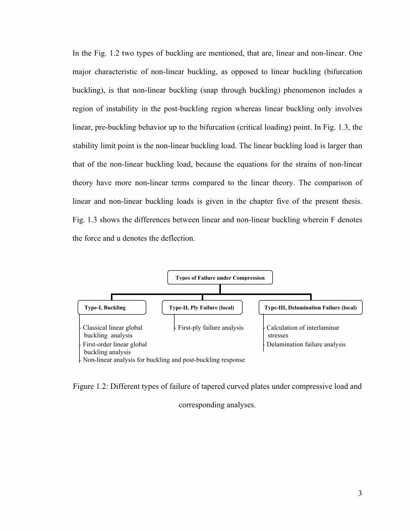
above mentioned behavior of structures can be called as Type-I, Type-II and Type-III

failures, which are caused by buckling, ply failure and delamination respectively. The

failure types and the corresponding analyses are shown in the Fig. 1.2.

Compressive Load X

Z

3

In the Fig. 1.2 two types of buckling are mentioned, that are, linear and non-linear. One

major characteristic of non-linear buckling, as opposed to linear buckling (bifurcation

buckling), is that non-linear buckling (snap through buckling) phenomenon includes a

region of instability in the post-buckling region whereas linear buckling only involves

linear, pre-buckling behavior up to the bifurcation (critical loading) point. In Fig. 1.3, the

stability limit point is the non-linear buckling load. The linear buckling load is larger than

that of the non-linear buckling load, because the equations for the strains of non-linear

theory have more non-linear terms compared to the linear theory. The comparison of

linear and non-linear buckling loads is given in the chapter five of the present thesis.

Fig. 1.3 shows the differences between linear and non-linear buckling wherein F denotes

the force and u denotes the deflection.

- Classical linear global buckling analysis

- First-ply failure analysis - Calculation of interlaminar stresses

- First-order linear global buckling analysis

- Delamination failure analysis

- Non-linear analysis for buckling and post-buckling response

Figure 1.2: Different types of failure of tapered curved plates under compressive load and

corresponding analyses.

Types of Failure under Compression

Type-I, Buckling Type-II, Ply Failure (local) Type-III, Delamination Failure (local)

4

Figure 1.3: Non-linear versus linear buckling behavior.

1.2 LITERATURE REVIEW

In the following, a review of existing works on the i) analysis of tapered composite

structures, ii) linear buckling analysis of shells, iii) analysis of shells using Ritz method,

vi) buckling analysis of shells using finite element method, v) first-ply failure analysis of

composite structures, vi) interlaminar stress and delamination failure analyses of

composite structures, vii) non-linear buckling analysis of shells, and viii) prediction of

critical load, is given.

1.2.1 Analysis of Tapered Composite Structures

A review of recent developments in the analysis of tapered laminated composite

structures with an emphasis on interlaminar stress analysis, delamination analysis and

parametric study has been presented by He et al [1]. From earlier research works

concerning this type of structure, two major categories of work on tapered composites

5

can be identified. The first is to understand failure mechanisms encompassing the

determination of the interlaminar stresses in the vicinity of ply drop-off, the calculation of

strain-energy release rate associated with delamination within the tapered region, and the

direct modeling of delamination progression by using finite elements. A large number of

investigators have been engaged in conducting research on this subject. The list includes

the works of Curry et al [2] and Hoa et al [3]. The second category is the investigations of

the parameters of the tapered composite structures that have substantial influences on the

structural integrity. Parametric studies of tapered composites were conducted by Daoust

and Hoa [4], Llanos and Vizzini [5], and Thomas and Webber [6].

A limited number of scientists have conducted research on tapered composite curved

plates. Piskunov and Sipetov [7] have proposed a laminated tapered shell structure which

accounts for the effects produced by transverse shearing strain. They have developed a

shearing strain model to minimize the differences between the physicomechanical

parameters (the values of the elasticity modulus, the shear modulus, the Poisson ratio, the

thermal conductivity coefficient, the linear expansion coefficient, etc.) of the composite

layers. Another work on tapered laminated shell structure was conducted by Kee and Kim

[8], where the rotating blade is assumed to be a moderately thick, width-tapered in

longitudinal direction and open cylindrical shell that includes the transverse shear

deformation and rotary inertia, and is oriented arbitrarily with respect to the axis of

rotation to consider the effects of disc radius and setting angle. The finite element method

is used for solving the governing equations.

6

1.2.2 Linear Buckling Analysis of Shells

A brief history of shell buckling is discussed by Lars and Eggwertz [9]. Euler’s formulae

for determining the critical load of a compressed straight bar were published in the

middle of the 18th century. The theory was further developed during the latter half of the

19th century, when the stability of thin plates was also analyzed in an analogous way,

Lars and Eggwertz [9]. A theory of shell buckling was first proposed in the beginning of

the 20th century, by Lorenz [10] and Timoshenko [11], who presented solutions for

axially compressed circular cylindrical shells. Ambartsumyan [12] has pioneered the

anisotropic thin shell analysis and he has also considered the local stability and vibration

in his formulations. Viswanathan et al [13] investigated elastic stability of thin laminated,

flat and curved, long rectangular plates subjected to combined in-plan loads. Hilburger

and Starnes [14] have worked on buckling behavior of compression-loaded composite

thin cylindrical shells with reinforced cutouts. Michael [15] has presented non

dimensional parameters and equations for buckling of symmetrically laminated thin

elastic shallow shells.

R. C. Tennyson [16] has conducted a brief review on static buckling theory for both

geometrically perfect and imperfect anisotropic composite circular thin cylinders for

various loading configurations. For comparison purposes, relevant experimental data are

discussed, including combined loading test results and recommendations are made

concerning the design of composite cylinders. A review work on the problem of buckling

of uniform-thickness and moderately-thick, laminated, composite shells subjected to

destabilizing loads has been carried out by Simitses [17]. The loads consist of uniform

7

axial compression, uniform lateral pressure and torsion applied individually or in

combination. The analysis is based on higher-order shear deformation (HOSD) shell

theory and/or first-order shear deformation (FOSD) shell theory with or without a shear

correction factor. Recommendations are also given for the moderately thick laminated

shells to check the failure strength, delamination initiation and growth and their effect on

the critical buckling loads.

1.2.3 Analysis of Shells Using Ritz Method

The problems of mechanics are solved by exact analytical methods, or approximate

methods (energy methods, variational methods, numerical methods). First preference is

given to exact solution; if it is not possible due to complexity of the structure then

‘approximate analytical or numerical solutions’ are used. The variational methods of

approximation include those of Rayleigh and Ritz, Galerkin, Petrov-Galerkin (weighted-

residuals), Kantorovich and the Finite Element Method (numerical method) which is a

“piecewise” application of the Ritz and Galerkin methods. Analytical solutions such as

Ritz solutions are of growing interest among scientists.

Buragohain and Velmurugan [18] have developed an energy-based smeared stiffener

model (SSM) to obtain equivalent stiffness coefficients of a composite lattice cylindrical

thin shell with hexagonal lattice patterns. Using the equivalent stiffness coefficients,

buckling analysis is carried out using Ritz method. Extensive finite element modeling

covering different sizes have also been carried out to compare the buckling results with

that of the Ritz method. Wong et al [19] have developed an analytical model using Ritz

8

method for the instability of orthotropic thin composite tubes subject to biaxial

compressive loads under clamped-clamped boundary conditions. Six E-glass woven

fabric-epoxy composite tubes with the same internal radius and different thicknesses and

longitudinal lengths were fabricated and subjected to various combinations of external

hydrostatic pressure and axial compressive load simultaneously. They have concluded

that the buckling envelopes in normalization form provide useful design data on the

strength of orthotropic composite tubes under a realistic range of biaxial loading

conditions.

Rao and Meyer-Piening [20] have conducted the buckling analysis of a simply supported

and uniform-thickness fiber reinforced plastic (FRP) faced cylindrical anisotropic

sandwich panel subjected to combined action of axial compression and bending and shear

using the Rayleigh-Ritz method. The values of the buckling coefficient are evaluated by

varying the aspect ratio, fiber orientation angle, core-to-face thickness ratio, radius of

cylindrical edge, bending load coefficient and shear load coefficient. Jaunky and Knight

[21] have obtained buckling loads of uniform-thickness circular cylindrical composite

panels using Sanders-Koiter’s, Love’s and Donnell’s shell theories with first-order shear-

deformation approach and Rayleigh-Ritz method that accounts for different boundary

conditions and material anisotropy. Results obtained using the shell theories are

compared with those obtained from finite element simulations, where the curved panels

are modeled using nine node quadrilateral continuum based shell elements that are

independent of any shell theory. The authors have compared the results obtained using

Ritz method with that of the finite element method and have concluded that Donnell’s

9

theory could be in error for some lamination schemes and geometrical parameters. Barai

and Durvasula [22] have studied the vibration and the buckling of uniform-thickness and

simply-supported curved plates, made of hybrid (Graphite/epoxy, Kevlar/epoxy and

Glass/epoxy) laminated composite materials, using first-order shear deformation theory

and Reissner's shallow shell theory. The natural frequencies and critical buckling loads

are calculated using Ritz method. The effects of curvature, aspect ratio, stacking

sequence and ply-orientation are studied.

1.2.4 Buckling Analyses of Shells Using Finite Element Method

Since the time of mid-1960s when the curved shell finite elements were invented, the

published literature on modeling of plates and shells analysis of structures has grown

extensively. In the last four decades, numerous theoretical models have been developed

and applied to various practical circumstances. It may be reasonable to state that no

single theory has proven to be general and comprehensive enough for the entire range of

applications. The pros and cons of different finite elements have been evaluated by the

several reviewers. Yang et al [23] have reviewed the advances of the formulations for

thin shell finite elements in the form of flat plates, axisymmetrical shells and curved

shells. They also illustrated with some extensions and applications to cases such as static

and dynamic responses, static and dynamic bucklings, laminated composites, random

loadings and random structural and material properties. The review work of Kapania [24]

deals with the development of various theories of modeling the thick laminated shells,

development of various finite elements to model these shells, buckling and post-buckling

analyses of perfect and imperfect laminated shells, and vibration and dynamic response

10

analyses of various laminated shells. Gilewski [25] has surveyed about 350 publications

related to the finite element models of moderately thick shells, concentrating on those

related to consistent displacement and stress/mixed/hybrid models. Noor and Burton [26]

have assessed the computational models for multilayered composite shells. In their work,

they have listed several references on finite element analysis of shells. Reddy and

Robbins [27] have presented a review work on equivalent-single-layer and layerwise

laminated plate theories, and their finite element models. Mackerle [28] has surveyed the

linear and non-linear, static and dynamic analyses of structural elements; his listed papers

have been published between 1992 and 1995. Yang et al [29] have summarized the

important literature on shell finite elements over 15 years (1985-2000). Their survey

includes the degenerated shell approach, stress-resultant-based formulations and Cosserat

surface approach, reduced integration with stabilization, incompatible modes approach,

enhanced strain formulations, 3-D elasticity elements, drilling degree of freedom

elements, co-rotational approach, and higher-order theories for composites.

Nine-node shell elements have advantages compared to eight-node elements. Nine-node

elements can pass the constant curvature patch test with bilinear element geometry while

eight-node shell elements cannot. A comparative study between these two types of

elements has been carried out by MacNeal and Harder [30]. Parisch [31] has discussed

special aspects of the nine-node Lagrange element. A modification of the stiffness is

proposed which allows the application of the element like a Kirchhoff-type model to any

plate problem. A case study of a variety of proposed element models is presented, and the

accuracy is shown for various plate and shell problems. Belytschko et al [32] have

11

described the implementation of a nine-node Lagrange element with uniform reduced

quadrature and spurious mode control for plates and shells. They have compared their

results with that of full integration and selective reduced integration versions of the

element. Lee and Hobbs [33] have suggested an automatic adaptive refinement procedure

for the analysis of shell structures using the nine-node degenerated solid shell element.

Chang et al [34] have examined a nine-node Lagrange shell element using a strain-based

mixed method. Kebari and Cassell [35] have presented a nine-node degenerate stress-

resultant shell element with six degrees of freedom at each node. Yeom et al [36] have

combined a nine-node shell element based on the assumed displacement formulation and

an eight-node shell element based on a modified version of the Hellinger-Reissner

principle with assumed linear transverse shear strain in order to eliminate locking . The

results of their analysis are compared with the classical thin plate theory and other

reference solutions. Jayasankar et al [37] have extended a nine-node degenerated shell

element developed earlier for stress analysis to the free vibration analysis of thick

laminated composites. In the present thesis work, a nine-node Lagrange shell element is

used.

MacNeal [38] has examined the cause of failure of finite elements and its remedy. It

includes quantitative analyses of failure modes and illustrations of possible side effects

found in proposed remedies, providing a practical understanding of finite element

performance. This book is designed to enable users and practitioners to identify and

circumvent the major flaws of finite elements, such as locking, patch-test failure,

spurious modes, rigid-body failure, induced anisotropy and shape sensitivity. Chapellet

12

and Bathe [39] have presented fundamental considerations regarding the finite element

analysis of shell structures.

1.2.5 First-ply Failure Analysis of Composite Structures

Reddy and Pandey [40] have developed finite-element computational procedure for the

first-ply failure analysis of composite plates. The procedure is based on the first-order

shear deformation theory and a tensor polynomial failure criterion that contains the

maximum stress, maximum strain, Hill, Tsai-Wu and Hoffman failure criteria. According

to their conclusions, all failure criteria that they have analyzed are equivalent in

predicting the failure when laminates are subjected to in-plane loads. For laminates

subjected to transverse load, the maximum strain and Tsai-Hill criteria predict different

failure location. Tsai [41] has compared the popular failure criteria of fiber-reinforced

composite materials. These criteria are empirical and should only be judged from the

standpoint of the fitness to data and the ease of application. The criteria for orthotropic

plies of unidirectional composites are extensions of those for isotropic materials. The

quadratic criteria are considered to be the most suitable for both isotropic and composite

materials. Macroscopic criteria are essential for design and for providing guidelines for

materials improvements. He has concluded that the failure criteria for multidirectional

laminates are valid up to the first-ply failure (before transverse cracking and delamination

occur). Nahas [42] has reviewed the existing theories of failure of laminated fiber-

reinforced composite materials. He has mentioned that there exist at least 30 failure

theories for laminated composites. Some of these theories are applied directly to the

laminate while the rest of the theories are applied to the individual layers of the laminate.

13

In addition, he has reviewed the theories of the post-failure behavior of laminated

composites, that is, the behavior of laminated composites beyond first-ply failure. For

post-failure analysis there exist at least twelve theories, which are included in his survey.

The World-Wide Failure Exercise (WWFE) contained a detailed assessment [43] of 19

theoretical approaches for predicting the deformation and failure response of polymer

composite laminates when subjected to complex states of stress. The leading five theories

(Zinoviev, Bogetti, Puck, Cuntze and Tsai) are explored in greater detail to demonstrate

their strengths and weaknesses in predicting various types of structural failure. According

to the investigations of WWFE, Tsai-Wu theory is the best one that can be used to predict

the first-ply failure of unidirectional laminates and any of the above mentioned five

failure theories can be used for multidirectional laminates. In the present thesis work,

Tsai-Wu failure theory is used to predict the first-ply failure of tapered curved plates.

1.2.6 Interlaminar Stress and Delamination Failure Analyses of Composite

Structures

Interlaminar stress analysis can be divided into four distinct categories: considering an

isotropic thin resin layer at the middle of two plies, analytical solutions obtained from

equilibrium equations, numerical solutions and layerwise theory. Mortensen [44], He et al

[45], and Fish and Lee [46] have analyzed the laminates using embedded resin layer.

Analytical solutions include the works of Kassapoglou [47], and Waltz and Vinson [48].

Pipes and Pagano [49] have employed finite-difference solution techniques for

interlaminar stresses in the composite laminates under uniform axial extension. Results

for material properties typical of a high modulus graphite-epoxy composite material

14

system are presented which explain the mechanism of shear transfer within a symmetric

laminate. Curry [50], and Ganesan and Liu [51] have carried out the investigation of

interlaminar stresses using finite element method. To accurately calculate the in-plane

and transverse stresses, without integrating the equilibrium equations, Reddy's [52]

layerwise theory can be used. Kant and Swaminathan [53] have reviewed the different

methods used for the estimation of transverse/interlaminar stresses in laminated

composite plates and shells. Both analytical and numerical methods are considered. The

aspects considered by them are: effects of variation in geometric and material parameters,

transverse shear and normal deformation, interface stress continuity and the interfacial

bonding on the accuracy of prediction of transverse/interlaminar stresses. Salamon [54]

has presented a review and assessment of the interlaminar delamination problem common

to layered composite materials. The work covers calculation of interlaminar stresses from

a homogeneous and microstructural material viewpoint. The observation of edge

delamination and experimental efforts are discussed together with the fracture mechanics

studies.

A large-size defect, or stress concentration is the primary cause of delamination. The

manufacturing errors or in-service and accidental loads lead to the delamination of the

laminates. Dropped plies result in an abrupt change of thickness and produce a

concentration of stresses which may cause delamination as explained by Curry [50]. The

Compression After Impact (CAI) refers to the sequence of events whereby a low velocity

transverse impact on a composite plate may also be the cause of internal delaminations.

When the plate is subsequently loaded by in-plane compression, local buckling may

15

occur around these delaminations, reducing the residual compressive strength of the

plate. Publications focusing on the after-impact evaluation and on the after-impact repair

of damaged structures are reviewed by Resnyansky [55]. Bolotin [56] has distinguished

two kinds of delaminations, depending on their position in a structural member.

Delaminations situated within the bulk of the material are rather like the cracks studied in

conventional fracture mechanics. The edge delaminations in thick members may also be

partially attributed to this type of delamination. Delaminations situated near the surface

of a structural member are a special kind of crack-like defect. The behavior of surface

delaminations is accompanied by their buckling. The local instability and crack growth

may produce the global instability of structural components such as columns, plates and

shells under compression. Therefore, he suggested the joint analysis of damage, fracture,

local buckling and global stability to predict the load-carrying capacity of composite

structures with delaminations. Bolotin [57] has surveyed the literature and the mechanical

aspects of delaminations in laminate composite structures. He discussed the surface and

internal delaminations of various origin, shape and location. He also analyzed the

origination, stability, and post-critical behavior of delaminations under quasi-static,

cyclic, and dynamic loads.

In the present thesis work, interlaminar stresses are analyzed using the two methods:

considering an isotropic thin resin layer at the middle of two plies and numerical

solutions. Using the later, the origination of delamination, if any, is analyzed. But the

local instability and crack growth are not considered in the present analyses. Considering

the above mentioned isotropic thin resin layer, transverse interlaminar normal and shear

16

stresses developed at the locations of the ply drop-off are also calculated to see the stress

state at those locations.

1.2.7 Non-linear Buckling Analysis of Shells

Linearized formulations are insufficient to explain and to account for many important

phenomena such as the effect of large deformations, amplitude-dependent frequency, the

catastrophic jump phenomena, subharmonic oscillations, and post-buckling behavior of

structures. In large-deflection (non-linear) theory, the deflections are assumed to be finite

though small. They are relatively large, however, when compared with that of small-

deflection theory. The strain-displacement relations include non-linear terms and

therefore the equilibrium equations in terms of displacements are non-linear in nature.

Donnell and Wa [58], in their approximate analysis of the effects of initial imperfections

on the buckling behavior of compressed cylinders, derived a set of large-deflection

equilibrium equations which is an extension of that derived by Von-Karman [59] for

large deflections of flat plates. Donnell and Wa [58] are the first to suggest a simple non-

linear theory for analyzing the stability of cylindrical shells.

Two distinct approaches have been followed in the literature in developing non-linear

finite element analysis of laminated structures: i) laminate theory and ii) 3-D continuum

formulation. In the laminate theory, the 3-D description is reduced to a 2-D description

based on the assumption of small strains and moderate rotations, no change of geometry

during loading, and the geometric non-linearity is in the form of Von-Karman strains.

Analysis based on this theory can be found in the Ref. [60]. In the 3-D continuum

17

formulation full non-linear strains or only the Von-Karman non-linear strains are

included as desired. There are two incremental continuum formulations that are used to

determine the deformation and stress states: a) the total Lagrangian formulation in which

the Green-Lagrange strain tensor and 2nd Piola-Kirchhoff stress tensor are used, and b)

the updated Lagrangian formulation in which the Cauchy stress tensor and the

infinitesimal Almansi strain tensor are used. Liao and Reddy [61] and Reddy [62] have

investigated shell structures using 3-D continuum formulation. In the present thesis work,

laminate theory is used in the formulation of non-linear buckling analysis.

In the literature five types of solution methods have commonly been used to solve the

non-linear problems of shell theory: i) The small parameter method, ii) The successive

approximation method, iii) the Picard iteration (or direct iteration) method, iv) the

Newton-Raphson iteration method, and v) the Riks method (or the incremental/iterative

solution method). The small parameter method was used by Kayuk [63-64]. The

successive approximation method was used by Vorovich [65-66] in the non-linear shell

theory to prove the solvability of boundary value problems. To the iteration algorithms

used in the vicinity of regular shell states belong the Newton and Raphson methods [67-

68], which are based on the idea of linearization [69] in which one constructs a linearized

operator at each iterative step. The convergence of Newton's method depends to a large

extent on how successfully the initial approximation of the deformation matrix has been

selected. This method was used in the Refs. [70] and [71] to solve the problems of shell

theory. Application of Newton-Raphson method to complex structural systems has been

carried out by Haeseler and Peitgen [72]. Originally and independently Riks [73] and

18

Wempner [74] proposed the earliest version of arc-length method. This arc-length

method is also known as incremental/iterative solution method. Based on the

conventional arc-length method, an improved arc-length method was proposed by Zhu

and Chu [75]. Bruce and Siegfried [76] have introduced a general formulation for all arc-

length procedures. They have also compared their results with that of the Crisfield’s

procedure [77]. Concerning the incremental strategies to solve the non-linear set of

algebraic equations, a new arc-length-type method was formulated by Carrera [78]. In

this work, he has compared the various types of path-following methods: the load control,

the displacement control, and the arc-length-type methods. In the present non-linear

analyses, the Crisfield’s procedure [77] is applied.

To investigate the non-linear deformation and stability of shell structures, it is convenient

to apply the Bubnov-Galerkin method [79]. Its implementation in the non-linear shell

stability problems has been discussed by Vol'mir [80]. Karman and Tsien [81]

implemented the non-linear statement of the problem for smooth cylindrical shells by

using the Donnell’s equations. The review studies related to further development of

stability investigations are contained in the monographs of Vol'mir [80] and Grigolyuk

and Kabanov [82]. Riks [83] and Ramm [84] have given an overview of different path-

following methods with a broad literature review. Sze et al [85] have presented popular

benchmark problems for geometric non-linear analysis of shells wherein eight sets of

popularly employed benchmark problems were proposed and solved. Andrade et al [86]

have formulated and implemented an eight-node hexahedral isoparametric element with

one-point quadrature for the geometrically non-linear static and dynamic analysis of

19

plates and shells made of composite materials. Han et al [87] have presented the

formulation of a non-linear composite nine-node modified first-order shear deformable

element-based Lagrangian shell element for the solution of geometrically non-linear

analysis of laminated composite thin plates and shells. Pradyumna et al [88] have

employed a higher order finite element formulation for the non-linear transient analysis

of functionally graded curved panels.

1.2.8 Prediction of Critical Load

Three types of buckling loads were defined by Chang and Chen [89], and Li [90]. These

three types of buckling loads include, i) the classical buckling load (the bifurcation point

or linear buckling load) of an ideal linear elastic structure, ii) the linearized buckling load,

and iii) fully non-linear buckling load. The basic assumption of the linearized buckling

analysis is that the structure behaves linearly before the critical load is reached. The

linearized buckling load is estimated on a stressed structure under a certain load and

considering the singularity of the tangent stiffness matrix. The details of the calculation

of linearized buckling load are explained in the book of Bathe [91]. The fully non-linear

buckling analysis employs a non-linear static analysis with gradually increasing loads to

seek the load level at which the structure becomes unstable which is known as the

stability limit load (snap through buckling). There have been few studies into the

effectiveness of the above-mentioned different types of buckling loads. Batdorf [92] first

idealized the cylindrical shell structure by neglecting the pre-buckling rotation and the

hoop stress and calculated the critical stress for the axially loaded cylinders. Croll [93]

has estimated the lower bound for the critical loads of cylindrical shells by neglecting the

strain energy due to membrane action of the structure. Brush [94] has considered the

20

effect of pre-buckling rotations and improved the Batdorf’s approximation [92]. Li [90]

has assumed the linear relation of load-displacement in pre-buckling state. He has also

presented a survey of concepts and methods that have been used in the non-linear

analysis of instability and collapse of structures. Almroth and Brogan [95] have discussed

the practical applicability of the bifurcation buckling theory. Several example cases were

presented in which results from a bifurcation buckling analysis were compared to the

results obtained from a rigorous non-linear analysis.

An improved scheme for critical load prediction has been developed by Brendel and

Ramm [96] using the total Lagrangian formulation. Based on their methodology, Chang

and Chen [89] combined the linear buckling loads with the loads obtained based on the

minimum number of non-linear analyses to predict the critical loads of shell structures.

They have estimated stability limit load by predicting and using the various linearized

critical loads corresponding to respective pre-stress loads (in their analysis a pre-stress

load is considered as the base load). In the present work, an improved methodology for

the prediction of stability limit load is developed that requires the consideration of only

two load steps instead of several load steps as in the case of existing methodology.

1.3 OBJECTIVES OF THE THESIS

None of the previously mentioned authors has worked on the response characteristics of

tapered curved composite plates under compression. In the present thesis work, this

response is considered for the purpose of studying the fundamental behavior of tapered

curved composite plates. On the other hand, a large number of load steps are required to

21

calculate the stability limit load from the conventional non-linear load-deflection curve.

A simplified methodology is introduced using two load steps to calculate the stability

limit load of a curved plate.

In the present thesis work, the buckling response of curved laminated plates with

longitudinal internal ply-drop-off configuration is investigated. Longitudinal ply-drop-off

tapers are identified as those in which the internal discontinuities of the laminate are

parallel to the direction of the applied load. Taking account the findings of He et al [1],

and Daoust and Hoa [4], different types of longitudinal cross sections as shown in Fig.

1.4 are investigated. In the Fig. 1.4, htk and htn denote the thicknesses at the thick end and

thin end respectively; Ltk, Ltap and Ltn denote the lengths of thick, taper and thin section

respectively; R, b and b’ denote the radius, the width and the cord of curved plates

respectively; and (uo, vo, wo) denotes the mid-plane displacement field with reference to

the global coordinate system (x, y, z). The taper configuration A is a simplified taper

configuration having only one large resin pocket. The taper configuration B has five

resin pockets: four small resin pockets are distributed symmetrically with respect to mid-

plan and the fifth one is designed combining the two small resin pockets. Every small

resin pocket is formed by dropping-off three composite plies and there are continuous

composite plies above and below each resin pocket. The hybrid configuration is modeled

combining the uniform-thickness and tapered sections as shown in the Fig. 1.4.

The first objective of the present thesis work is to conduct the linear global buckling

analysis of the tapered curved plates shown in Fig. 1.4 using Ritz method. Linear global

22

buckling analysis includes the classical and first order shear deformation shell theories.

For the buckling analysis based on classical shell theory, namely Donnell’s, Love’s,

Mushtari’s, Timoshenko’s, Vlasov’s, Sander’s, Koiter’s and Novozhilov’s theories are

used. Six shell theories are used in the analysis based on first-order shear deformation

theory, namely Donnel’s, Love’s, Moreley’s, Loo’s, Sander’s and Koiter’s theories. The

relative efficiency and accuracy of these shell theories are assessed based on critical

buckling loads obtained using Ritz method and finite element method. Buckling analysis

results obtained using Ritz method are compared with the existing experimental and

analytical results, and are also evaluated with that of the results obtained using ANSYS.

The second objective is to determine the failure loads corresponding to local material

failure of the tapered curved plates using ANSYS®. The first-ply failure load is calculated

considering the first instance at which any layer or more than one layer fails at the same

load. The initiation of delamination, if any, is analyzed using the transverse interlaminar

stresses under compressive load. The third objective is to determine the critical sizes and

parameters of the tapered curved plates based on the failure and buckling analyses. The

fourth objective is to evaluate the stability limit load and ultimate strength of the tapered

curved plate beyond the initial buckling. The mechanical structures undergo large

deflection after they buckle. The effect of large deflection is considered in the non-linear

analysis. A simplified methodology for non-linear buckling analysis is introduced to find

out the stability limit load which requires only two load steps instead of large number of

load steps. Non-linear buckling analysis is carried out using FEM. A parametric study

that encompasses the effects of boundary conditions, stacking sequence, taper

23

configurations, radius and other geometric parameters of the plate is conducted. Finally,

design guidelines for the tapered curved composite plates are established.

Figure 1.4: Different longitudinal cross sections of curved plate.

1.4 LAYOUT OF THE THESIS

In the present chapter, a general discussion about the compressive strength of tapered

curved composite plates, literature review on the a) analysis of tapered composite

structures, b) linear buckling analysis of shells, c) analysis of shells using Ritz method, d)

buckling analysis of shells using finite element method, e) first-ply failure analysis of

composite structures, f) interlaminar stress and delamination failure analyses of

composite structures, g) non-linear buckling analysis of shells, and h) prediction of

Taper Configuration A

Taper Configuration B

Ltap

htnhtk

Ltk Ltap Ltn

b

R

z,wo

x,uo

y,vo

Hybrid Configuration with Tapered andUniform-thickness Sections

24

critical load, objectives of the present thesis, and finally, the layout of the present thesis,

are given.

In chapter two, the Ritz method and eight classical shell theories are used for the global

linear buckling analysis of thickness-tapered curved composite plates subjected to

uniaxial compressive load. The results that obtained using Ritz method are compared

with that of the existing studies. Finally, a parametric study is carried out.

In chapter three, the Ritz method is used for the global buckling analysis based on six

first-order shear deformation shell theories. To apply the first-order shear deformation

shell theories to analyze the plates, an appropriate set of shear correction factors have

been determined. The critical sizes and parameters of the tapered curved plates that will

not fail before global buckling are determined. At the end, a parametric study is

accomplished.

In chapter four, a nine-node tapered curved finite element is developed based on six first-

order shear deformation shell theories. To apply the first-order shear deformation shell

theories to analyze the tapered plates, an appropriate set of shear correction factors have

been determined. Various boundary conditions are considered for different laminate and

lay-up configurations. The buckling loads obtained using FEM are also compared with

that of the existing experimental and analytical results. At the end, a parametric study is

concluded.

25

In chapter five, non-linear buckling analysis is carried out using finite element method.

To find out the stability limit load, a simplified methodology is introduced which requires

only two load steps. Three types of plates are analyzed: uniform curved, tapered curved

and hybrid (uniform and tapered) curved plates.

In chapter six, conclusions, a summary of contributions, and suggestions for the future

work are given.

26

Chapter 2

Compressive Response of Thickness-Tapered Shallow Curved

Composite Plates Based on Classical Shell Theory

2.1 INTRODUCTION

In this chapter, the compressive response of shallow curved composite plates with

longitudinal internal ply-drop-off configurations is investigated. The Ritz method is used

for the global buckling analysis considering uniaxial compressive load. Linear buckling

analysis is carried out based on eight well-known classical shallow shell theories, namely

Donnell’s, Love’s, Mushtari’s, Timoshenko’s, Vlasov’s, Sander’s, Koiter’s and

Novozhilov’s theories. The strength characteristics and load carrying capability of the

tapered curved plates are investigated considering the first-ply failure analysis using

ANSYS®. Based on the failure and buckling analyses, the critical sizes and parameters of

the tapered curved plates that will not fail before global buckling are determined. A

parametric study is conducted that encompasses the effects of boundary conditions,

stacking sequence, taper configurations, radius, and geometric parameters of the plates.

2.2 FORMULATION

Total potential energy criterion is used in order to analyze the stability problems. The

curved plates of the Fig. 1.4 are considered to conduct the buckling analysis. Resin

pockets are assumed to be the combination of hypothetical resin plies. Following

assumptions are considered in the buckling analyses:

27

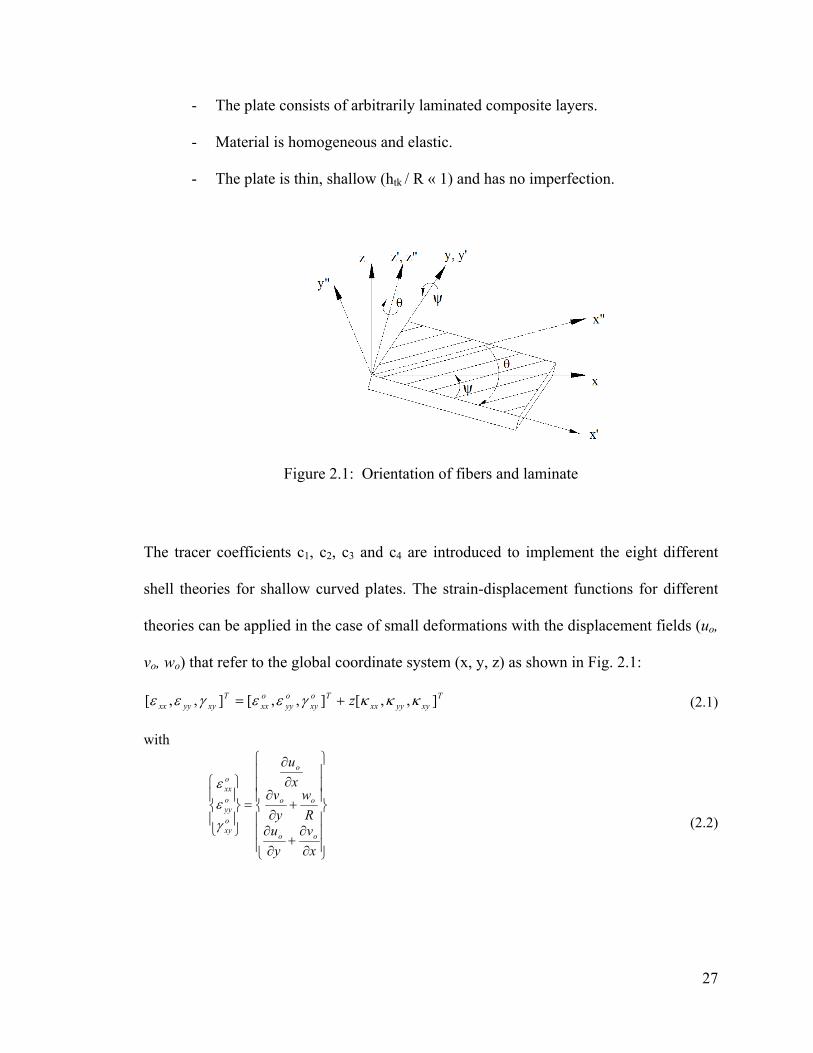
- The plate consists of arbitrarily laminated composite layers.

- Material is homogeneous and elastic.

- The plate is thin, shallow (htk / R « 1) and has no imperfection.

Figure 2.1: Orientation of fibers and laminate

The tracer coefficients c1, c2, c3 and c4 are introduced to implement the eight different

shell theories for shallow curved plates. The strain-displacement functions for different

theories can be applied in the case of small deformations with the displacement fields (uo,

vo, wo) that refer to the global coordinate system (x, y, z) as shown in Fig. 2.1:

Txyyyxx

Toxy

oyy

oxx

Txyyyxx z ],,[],,[],,[ κκκγεεγεε += (2.1)

with

⎪⎪⎪

⎭

⎪⎪⎪

⎬

⎫

⎪⎪⎪

⎩

⎪⎪⎪

⎨

⎧

∂∂

+∂∂

+∂∂

∂∂

=⎪⎭

⎪⎬

⎫

⎪⎩

⎪⎨

⎧

xv

yu

Rw

yv

xu

oo

oo

o

oxy

oyy

oxx

γεε

(2.2)

28

and

⎪⎪⎪

⎭

⎪⎪⎪

⎬

⎫

⎪⎪⎪

⎩

⎪⎪⎪

⎨

⎧

⎟⎟⎠

⎞⎜⎜⎝

⎛∂∂

−∂∂

+∂∂

∂−

∂∂

+−∂∂

−

∂∂

−

=⎪⎭

⎪⎬

⎫

⎪⎩

⎪⎨

⎧

yuc

xvc

Ryxw

yv

Rcw

Rc

yw

xw

ooo

oo

o

o

xy

yy

xx

43

2

221

2

2

2

2

12κκκ

(2.3)

where Txyyyxx ],,[ 000 γεε and T

xyyyxx ],,[ κκκ are the mid-surface strains and curvatures

respectively. The superscript ‘T’ stands for transpose of the matrix.

By setting,

i) c1 = c2 = c3 = c4 = 0, equations that correspond to Donnel’s [97],

Mushtari’s [97], Timoshenko’s [97] and Love’s [98] shell theories are obtained.

ii) c1 = c3 = c4 = 1 and c2 = 0, equations that correspond to Vlasov’s [99] shell

theory is obtained.

iii) c1 = c2 = 0 and c3 = c4=1/2, equations that correspond to Sander’s [100]

and Koiter’s [101] shell theories are obtained.

iv) c1 = c4 = 0, c2 =1 and c3 =2, equations that correspond to Novozhilov’s

[102] shell theory is obtained.

The Fig. 2.1 describes the orientation of fibers and laminate. """ , zandyx are the

principal material directions oriented by θ (fiber orientation angle) degrees with respect

to the ''' , zandyx directions respectively. The local coordinate system ( ''' ,, zyx ) makes

an angle of ψ (taper angle) degrees with the global coordinate system (x, y, z).

Hooke’s law for orthotropic materials in the principal material directions can be written

as:

29

⎪⎪⎪⎪

⎭

⎪⎪⎪⎪

⎬

⎫

⎪⎪⎪⎪

⎩

⎪⎪⎪⎪

⎨

⎧

⎥⎥⎥⎥⎥⎥⎥⎥

⎦

⎤

⎢⎢⎢⎢⎢⎢⎢⎢

⎣

⎡

=

⎪⎪⎪⎪

⎭

⎪⎪⎪⎪

⎬

⎫

⎪⎪⎪⎪

⎩

⎪⎪⎪⎪

⎨

⎧

""

""

""

""

""

""

""

""

""

""

""

""

66

55

44

332313

232212

131211

"000000"000000"000000"""000"""000"""

yx

zx

zy

zz

yy

xx

yx

zx

zy

zz

yy

xx

CC

CCCCCCCCCC

γγγεεε

τττσσσ

(2.4)

where ij"σ and ij

"τ are the normal stresses and shear stresses respectively and, ij"ε and

ij"γ are the normal strains and shear strains respectively with i, j = """ ,, zyx in the

material coordinate system ),,( """ zyx . etcCC ...., 12"

11" are the corresponding stiffness

coefficients.

Eq. (2.4) can be expressed as:

{ } [ ]{ }""" εσ C= (2.5)

The stress transformation matrix due to fiber orientation angle θ is of the following form

[103]:

[ ]

⎥⎥⎥⎥⎥⎥⎥⎥

⎦

⎤

⎢⎢⎢⎢⎢⎢⎢⎢

⎣

⎡

−−−

−

=

θθθθθθθθθθ

θθθθθθθθ

σθ

22

22

22

sincos000sincossincos0cossin0000sincos000000100

sincos2000cossinsincos2000sincos

T

(2.6)

The stress transformation matrix due to taper angle ψ can be written as:

[ ]

⎥⎥⎥⎥⎥⎥⎥⎥

⎦

⎤

⎢⎢⎢⎢⎢⎢⎢⎢

⎣

⎡

−−−

−=

ψψψψψψψψ

ψψψψψψ

ψψψψ

σψ

cos0sin0000sincos0sincos0sincos

sin0)cos(0000sincos20cos0sin0000100sincos20sin0cos

22

22

22

T

(2.7)

The elastic properties of a layer are given in its principal material directions by the Eq.

(2.4) but the final form of the governing equations are in the global coordinate system

30

(x,y,z). The layer properties should be transformed to global directions from the principal

material directions as follows:

--First, coordinate transformation corresponding to the rotation of x” and y” about z” axis

(see Fig. 2.1)

--Second, coordinate transformation corresponding to the rotation of x’ and z’ about y’

axis (see Fig. 2.1)

Therefore, the stress tensor for a ply in the tapered laminate is formulated as:

{ } [ ][ ][ ][ ] [ ] { }εσ σψσθσθσψTT TTCTT "= (2.8)

where [ σθT ] and [ σψT ] are the stress transformation matrices due to fiber orientation angle

θ and taper angle ψ respectively.

The above equation can be expressed in a short form:

{ } [ ]{ }εσ C= (2.9)

Thus, the stiffness matrix [C] in the global coordinate system ( zyx ,, ) can be expressed

by the stiffness matrix [C”] in the principal material coordinate system ( ","," zyx ) and

the transformation matrices as:

[ ] [ ][ ][ ][ ] [ ]TT TTCTTC σψσθσθσψ "= (2.10)

The reduced stiffness matrix is in the form:

⎪⎭

⎪⎬

⎫

⎪⎩

⎪⎨

⎧

⎥⎥⎥

⎦

⎤

⎢⎢⎢

⎣

⎡=

⎪⎭

⎪⎬

⎫

⎪⎩

⎪⎨

⎧

xy

yy

xx

xy

yy

xx

QQQQQQQQQ

γεε

τσσ

662616

262212

161211

(2.11)

where, Qij = Cij - Ci3 Cj3/ C33, i , j = 1,2,6 (2.12)

and Cij is the coefficient of material stiffness matrix in the global coordinate system given

by the Eq. (2.10).

31

The equations for coefficients of matrices [A], [B] and [D] for tapered laminate can be

written as

dzzzQDBAh

hijijijij ),,1(),,( 2

2/

2/∫

−

= i , j = 1,2,6 (2.13)

In which, Aij is the stretching stiffness matrix coefficient, Bij is the coupling stiffness

matrix coefficient, Dij is the bending stiffness matrix coefficient, and Qij is calculated

from the Eq. (2.12).

The strain energy of the tapered shell structure is written in Cartesian co-ordinates as

follows:

dxdyDBBAb L

Ttap

∫ ∫⎭⎬⎫

⎩⎨⎧

⎥⎦

⎤⎢⎣

⎡=∏

0 0

][][21 εε (2.14)

where Txyyyxxxyyyxx ],,,,,[][ 000 κκκγεεε = (2.15)

The potential energy due to the uniaxial compression is [104]:

dxdyx

wxv

xu

Fb L

oootap

∫ ∫⎪⎭

⎪⎬⎫

⎪⎩

⎪⎨⎧

⎥⎥⎦

⎤

⎢⎢⎣

⎡⎟⎠⎞

⎜⎝⎛∂∂

+⎟⎠⎞

⎜⎝⎛∂∂

+∂∂

−=0 0

22

21λ

(2.16)

where, λ is the inplane normal compressive load in x direction.

The approximate solutions for the displacements are expressed as a double series:

∑∑= =

=M

m

N

nnmmno yUxUUyxu

1 1)()(),(

(2.17)

∑∑= =

=M

m

N

nnmmno yVxVVyxv

1 1)()(),(

(2.18)

∑∑= =

=M

m

N

nnmmno yWxWWyxw

1 1)()(),(

(2.19)

32

The functions Um(x), Un(y), Vm(x), Vn(y), Wm(x), and Wn(y) are so chosen as to satisfy

the boundary conditions which are given in the Appendix A and the coefficients Umn, Vmn

and Wmn are determined by the following stationary conditions:

mnmn UF

U ∂∂

=∂∏∂ (2.20)

mnmn VF

V ∂∂

=∂∏∂ (2.21)

mnmn WF

W ∂∂

=∂

∏∂ (2.22)

where ∏ and F are given by the Eqs. (2.14) and (2.16) respectively.

The Eqs. (2.20) through (2.22) are, respectively, rewritten as:

[ ] [ ] [ ][ ] [ ] [ ] [ ][ ]⎪⎭

⎪⎬

⎫

⎪⎩

⎪⎨

⎧−=

⎪⎭

⎪⎬

⎫

⎪⎩

⎪⎨

⎧

IJ

IJ

IJ

IJ

IJ

IJ

IJIJIJ

WVU

WVU

LLL 000131211 λ (2.23)

[ ] [ ] [ ][ ] [ ] [ ] [ ][ ]⎪⎭

⎪⎬

⎫

⎪⎩

⎪⎨

⎧−=

⎪⎭

⎪⎬

⎫

⎪⎩

⎪⎨

⎧

IJ

IJ

IJ

IJ

IJ

IJ

IJ

IJIJIJ

WVU

GWVU

LLL 00 22232212 λ (2.24)

[ ] [ ] [ ][ ] [ ] [ ] [ ][ ]⎪⎭

⎪⎬

⎫

⎪⎩

⎪⎨

⎧−=

⎪⎭

⎪⎬

⎫

⎪⎩

⎪⎨

⎧

IJ

IJ

IJ

IJ

IJ

IJ

IJ

IJIJIJ

WVU

GWVU

LLL 33332313 00λ (2.25)

Eqs. (2.23) through (2.25) are rearranged into matrix form:

[ ] [ ] [ ][ ] [ ] [ ][ ] [ ] [ ]

[ ] [ ] [ ][ ] [ ] [ ][ ] [ ] [ ] ⎪

⎭

⎪⎬

⎫

⎪⎩

⎪⎨

⎧

⎥⎥⎥

⎦

⎤

⎢⎢⎢

⎣

⎡−=

⎪⎭

⎪⎬

⎫

⎪⎩

⎪⎨

⎧

⎥⎥⎥

⎦

⎤

⎢⎢⎢

⎣

⎡

IJ

IJ

IJ

IJ

IJ

IJ

IJ

IJ

IJIJIJ

IJIJIJ

IJIJIJ

WVU

GG

WVU

LLLLLLLLL

33

22

332313

232212

131211

0000000

λ (2.26)

Further details about the matrices ],[],[],[],[ 33221211IJIJIJIJ GGLL and so on are given in the

Appendix A. The eigenvalues λ are the values of buckling loads. The following indicial

expressions were introduced [105] and used in Eq. (2.26):

33

nMmI +−= )1( and jNiJ +−= )1( (2.27)

where Mmi ......2,1, = and Nnj ......2,1, = .

Eq. (2.26) can be written in the short form:

0][][ =+ ZK λ

(2.28)

where, [K] and [Z] are the stiffness matrix and geometric stiffness matrix respectively.

Eq. (2.28) is solved using MATLAB® program as an eigenvalue problem for which the

eigenvalues λ are the values of buckling loads. The smallest value of λ is the critical

buckling load, crλ .

2.3 VALIDATION

To the author’s knowledge, no results are available yet in the literature on the buckling

loads of the tapered curved composite plates under the action of uni-axial compression.

Therefore the comparison with the existing works could not be made. In order to validate

the formulation and analysis, first, the taper angle is set to be zero, and the resulting

uniform-thickness laminates have been analyzed and the results have been compared with

that available in the literature for the uniform-thickness laminates. For this purpose, a

uniform-thickness cylindrical panel made of Morganite II/4617 having the mechanical

properties of Ex” =137.89 x109 Pa (20.0 x106 psi), Ey” = 14.48 x109 Pa (2.1 x106 psi),

Gx”y” = 5.86 x 109 Pa (0.85x106 psi), υx”y” = 0.21 and the geometrical properties of length

L = 0.3048 m (12 inches), width b = 0.2032 m (8 inches), radius R = (0.3048 - h/2) m,

thickness h = 1.50368 x 10-03 m (0.0592 inches) and taper angle ψ = 0 degree which has

been investigated by Wilkins [106] is considered. The plate is clamped at four edges (C4-

C4) and the boundary conditions (C4-C4) are given in the Appendix A. In the work of

34

Wilkins [106], experiments were carried out applying the experimental procedures of

Southwell (S) and Moiré (Mo). Results of the present work are compared with that of the

Ref. [106] for different laminate configurations in the Tables 2.1 and 2.2.

From the Table 2.1 it is found that the result is converged when 9 terms are taken in the

Ritz series. Most of the buckling problems in the present work have converged with 9

terms. The results based on different shell theories are close to each other but the

Novozhilov’s theory provides the most conservative result. As can be seen from Tables

2.1 and 2.2, the present analytical results differ from that of the experimental ones with a

maximum error of 15.9 percent, which is nominal for a linear buckling analysis.

Table 2.1: The comparison of buckling load of uniform-thickness cylindrical panel

Laminate Configurat-ion

No. of Terms in the Series (N x M)

Wilkins [106] (x104 N/m)

Present (x 104 N/m) Donnell, Love, Doubly, Mushtari, Timoshenko

Vlasov Sander, Koiter Novozhilov

Exp. Ritz Solution Ritz Solution Ritz Solution Ritz Solution

[0/90]2s

1x1

15.5162 (S)

634.6769 633.2735 634.5210 632.3378 2x2 118.0114 117.7504 117.9824 117.5764 3x3 20.6453 20.5996 20.6402 20.5692 4x4 18.5656 18.5246 18.5611 18.4972 5x5 18.1300 18.0899 18.1255 18.0632 6x6 17.8980 17.8584 17.8936 17.8320 7x7 17.8629 17.8234 17.8585 17.7971 8x8 17.8235 17.7841 17.8191 17.7578 9x9 17.8191 17.7797 17.8148 17.7535

Table 2.2: The comparison of buckling loads for uniform-thickness cylindrical panel of

different configurations

Laminate Configuration Wilkins [106] (x 104 N/m)

Present, Novozhilov (x 104 N/m)

Exp. Ritz Solution [0/45/90/-45]s 15.5425 (Mo) 15.9825 [0]6s 47.1485 (S) 54.6658

35

Next, uniform-thickness cylindrical panel made of T300/5208 graphite/epoxy having the

mechanical properties of Ex” = 141.34 GPa (20.5 x106 psi), Ey” = 8.96 GPa (1.3 x106 psi),

Gx”y” = 5.17 GPa (0.75 x106 psi) and υx”y” = 0.335 which is clamped (C3) in transverse

direction and simply supported (S3) in longitudinal direction is considered. The boundary

conditions (C3-S3) are given in the Appendix A. The dimensions of the plate are taken to

be: length L = 0.3048 m (12 inches), the cord length 'b = 0.3048 m, radius of the plate R

= 0.3048 m, thickness h = 1.016x10-03 m (0.04 inches). Becker [107] has conducted the

bifurcation (obtained from eigenvalue solution) buckling analysis of this curved plate

using STAGS computer code. In the present study, the buckling analysis is carried out

using Ritz method based on various shell theories and the results are compared with that

given in the work of Becker [107]. The normalized buckling load is given in the Table

2.3 where crλ is the critical buckling load.

Table 2.3: The comparison of buckling loads of uniform-thickness curved plates applying

different shell theories

Laminate Configuration

Becker [107] )/()( 3

"2 hEL xcrλ Present )/()( 3

"2 hEL xcrλ

Theory Exp. Donnell, Love, Doubly Mushtari, Timoshenko Vlasov Sander,

Koiter Novozhilov

[90/0]2s 33.30 24.50 34.950 34.866 34.949 34.816

As can be observed from the Table 2.3, the present result is in good agreement with the

theoretical buckling load given in the reference work. The present results are higher than

that of the experimental results. According to Ref. [107], the bifurcation buckling loads

may be 23 to 45 percent higher than the experimental buckling results because the

occurrence of elastic instability is strongly influenced by the geometric nonlinearity,

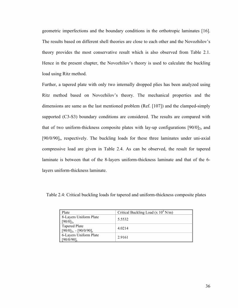
36

geometric imperfections and the boundary conditions in the orthotropic laminates [16].

The results based on different shell theories are close to each other and the Novozhilov’s

theory provides the most conservative result which is also observed from Table 2.1.

Hence in the present chapter, the Novozhilov’s theory is used to calculate the buckling

load using Ritz method.

Further, a tapered plate with only two internally dropped plies has been analyzed using

Ritz method based on Novozhilov’s theory. The mechanical properties and the

dimensions are same as the last mentioned problem (Ref. [107]) and the clamped-simply

supported (C3-S3) boundary conditions are considered. The results are compared with

that of two uniform-thickness composite plates with lay-up configurations [90/0]2s and

[90/0/90]s, respectively. The buckling loads for these three laminates under uni-axial

compressive load are given in Table 2.4. As can be observed, the result for tapered

laminate is between that of the 8-layers uniform-thickness laminate and that of the 6-

layers uniform-thickness laminate.

Table 2.4: Critical buckling loads for tapered and uniform-thickness composite plates

Plate Critical Buckling Load (x 104 N/m) 8-Layers Uniform Plate [90/0]2s

5.5532

Tapered Plate [90/0]2s - [90/0/90]s

4.0214

6-Layers Uniform Plate [90/0/90]s

2.9161

37

2.4 FIRST-PLY FAILURE ANALYSIS

The load carrying capability of the tapered curved plates is studied considering first-ply

failure load. This type of failure analysis is considered in the present work to determine

whether a layer has failed due to compressive loading before global buckling. The

commercial software ANSYS® has been chosen to model the curved composite plates.

Element SHELL99 is used for the first-ply failure analysis using ANSYS®. SHELL99 is

an 8-node, 3-D shell element with six degrees of freedom (three translations and three

rotations) at each node. It is designed based on the degenerated solid approach with shear

deformation effect and to model thin to moderately-thick plate and shell structures with a

side-to-thickness ratio of roughly 10 or greater. The tapered curved plates are meshed by

eighty-one elements which are shown by numbering in the Fig. 2.2. The first-ply failure

analysis is carried out using ANSYS® based on the 3-D version of Tsai-Wu failure

criterion. The first-ply failure refers to the first instant at which any layer or more than

one layer fails at the same load. The same criterion is applied for both the composite ply

and the resin pocket, the resin pocket is considered (imagined) to be made up of layers of

isotropic resin material. Material properties [45] of composite ply and epoxy are given in

the Tables 2.5 and 2.6 respectively, where Xt, Yt, Zt are the normal tensile strengths in the

principal material directions ","," zyx respectively; Ryz, Sxz, Txy are the shear strengths

in the y”z”, x”z”, x”y” planes respectively; Xc, Yc, Zc are the normal compressive strengths

in the principal material directions ","," zyx respectively.

38

Table 2.5: Material properties of NCT/301 graphite-epoxy composite material

Table 2.6: Material properties of epoxy material used in NCT/301

Mechanical Property Value Strength Property Value Ex” = Ey” = Ez” 3.930 GPa Xt = Yt = Zt 57.00 MPa Gx”y” = Gx”z” = Gy”z” 1.034 GPa Xc = Yc = Zc -104 MPa

"""""" zyzxyxννν == 0.370 Ryz = Sxz = Txy 22 MPa

Figure 2.2: Finite element mesh.

Four different sizes of square tapered composite plates with taper configuration B and

made of NCT/301 graphite-epoxy composite material is considered. The lay-up is

[0/90]9s at the thick end and [0/90]3s at the thin end which is defined as lay-up

Mechanical Property Value Strength Property Value Ex” 113.900 GPa Xt 1621 MPa

Ey” = Ez” 7.985 GPa Xc -1250 MPa Gx”y” = Gx”z” 3.137 GPa Yt = Zt 48.28 MPa

Gy”z” 2.852 GPa Yc = Zc -200 MPa """" zxyx

νν = 0.288 Ryz 25.00 MPa

""zyν 0.400 Sxz = Txy 33.30 MPa

39

configuration LC1 in the Table 2.7. The mechanical properties of the composite and

epoxy material are given in Tables 2.5 and 2.6 respectively. The geometric properties of

the plates are: side length of the square plates varies from 85.9 to 859.4 mm, plate

thickness at thick end htk = 4.5 mm and the radius R = 500 mm. The clamped-clamped

(C4-C4) boundary conditions given in the Appendix A are considered. The results of

failure analysis are tabulated in the Table 2.8.

Table 2.7: List of lay-up configurations

Lay-up Configuration

Ply Staking Sequence Lengths of the Hybrid Configuration (m)

Thick Section

Tapered Section

Thin Section

Thick Section

Tapered Section

Thin Section

LC1 [0/90]9s Config. B [0/90]3s 0.0382 0.1146 0.0382 LC2 [±45]9s Config. B [±45]3s 0.0382 0.1146 0.0382 LC3 [02/±458]s Config. B [02/±452]s 0.0382 0.1146 0.0382

Table 2.8: Critical buckling load and first-ply failure load of tapered curved laminates

with lay-up configuration LC1 and taper configuration B

Taper Angle in Degree

Side Length of the Square Plate (m)

Buckling Load Using Ritz Method

(x 104 N/m)

First-ply Failure Load Using ANSYS® (x 104 N/m)

Failure Location (FEN, FLN)*

0.10 0.8594 14.20 48.05 1, 2 0.50 0.1719 43.81 42.00 1, 2 0.75 0.1146 70.69 43.50 9, 3 1.00 0.0859 100.23 45.60 9, 3

* FEN and FLN denote the failed element number and failed layer number at first-ply failure.

The side length of square plates corresponding to taper angles is given in the Table 2.8.

The first-ply failure loads are compared with the buckling loads. As can be seen from the

40

Table 2.8, the tapered curved plates corresponding to taper angles of 0.50, 0.75 and 1.0

degrees will fail by first-ply failure before the global buckling. On the other hand, the

plate corresponding to taper angle of 0.1 degree will fail first by buckling failure.

Therefore, the maximum plate size should be (0.1754 x 0.1754) which is corresponding

to taper angle of 0.49 degree and the critical length-to-height ratio (Ltap / htk) is to be 38.9.

The failed layer numbers 2 and 3, respectively, are the second layer and the third layer at

the thick end of the plates. All the tapered curved plates failed at the thick end where the

minimum numbers of plies above or below the resin pockets.

Next, the tapered plates of the Table 2.8 are analyzed for different radii using the same

boundary conditions (C4-C4), ply-configuration (LC1) and material properties (Table 2.5

and Table 2.6). The critical sizes of the tapered curved plates are determined

corresponding to various radii. For the calculation of critical length-to-height ratio, the

same procedure is applied as mentioned in the previous problem for the radius of 500

mm. In the Fig. 2.3, radius versus critical length-to-height ratio of tapered curved plates is

plotted. In this figure, Ltap denotes the taper length and htk denotes the thickness at the

thick end. The stiffness of the tapered curved plate increases with the decrease of radius.

Therefore, critical length-to-height ratio is to be increased with the decrease of radius to

avoid the material failure. It can also be seen in the Fig. 2.3 that the critical length-to-

height ratio increases with the decrease of radius. The critical length-to-height ratio varies

non-linearly with the change of radius. The design limit of the tapered curved composite

plates with the lay-up configuration LC1 and the taper configuration B is determined and

represented as the hatched area in the Fig. 2.3. Beyond this limit, tapered curved plate

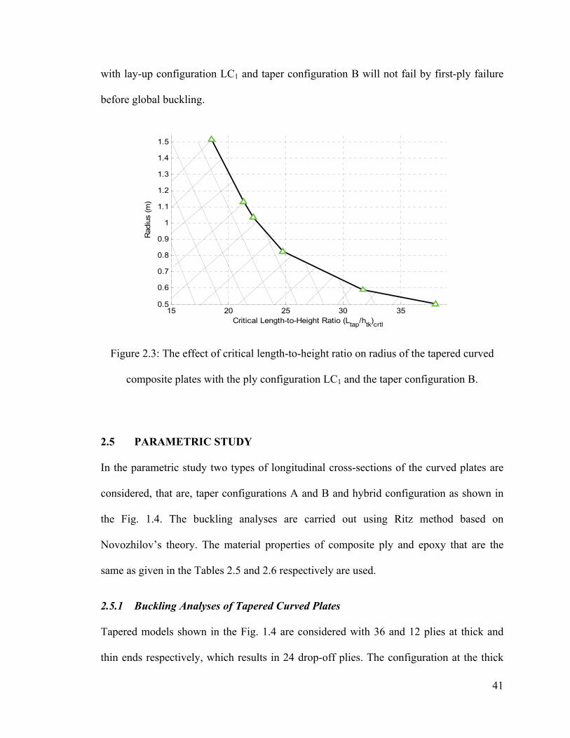
41

with lay-up configuration LC1 and taper configuration B will not fail by first-ply failure

before global buckling.

Figure 2.3: The effect of critical length-to-height ratio on radius of the tapered curved

composite plates with the ply configuration LC1 and the taper configuration B.

2.5 PARAMETRIC STUDY

In the parametric study two types of longitudinal cross-sections of the curved plates are

considered, that are, taper configurations A and B and hybrid configuration as shown in

the Fig. 1.4. The buckling analyses are carried out using Ritz method based on

Novozhilov’s theory. The material properties of composite ply and epoxy that are the

same as given in the Tables 2.5 and 2.6 respectively are used.

2.5.1 Buckling Analyses of Tapered Curved Plates

Tapered models shown in the Fig. 1.4 are considered with 36 and 12 plies at thick and

thin ends respectively, which results in 24 drop-off plies. The configuration at the thick

15 20 25 30 350.5

0.6

0.7

0.8

0.9

1

1.1

1.2

1.3

1.4

1.5

Critical Length-to-Height Ratio (Ltap/htk)crtl

Rad

ius

(m)

42

end is (0/90)9s, and that of the thin end is (0/90)3s; this lay-up configuration is defined as

LC1. In the analyses of taper configurations, the height of thick end htk = 4.5 mm and the

radius of curved plate R = 500 mm are considered. For the analyses of tapered curved

plates only LC1 ply-configuration with clamped-clamped (C4-C4) boundary conditions

are considered. Various parameters, namely ply drop-off, taper angle and length-to-radius

ratio are investigated to see the effects of these parameters on buckling load of tapered

curved plates. The results are shown in the following Figs. 2.4 through 2.6.

2.5.1.1 Influence of Ply Drop-Off

The effect of ply drop-off on critical buckling load is shown in the Fig. 2.4. To

investigate this effect, the side length of square tapered plate is considered as 859.4 mm

corresponding to taper angle of 0.1 degree. The thickness of the thick end is not changed

and the taper angle is varied with the corresponding increase in the number of drop-off

plies. The plate can be considered as a uniform-thickness plate when the number of ply

drop-off is set to zero and the taper configuration A is obtained by dropping-off twenty

four plies. The plates are clamped-clamped (C4-C4) at four edges and the lay-up

configuration is LC1. In the Fig. 2.4, crλ denotes the critical buckling load.

From the Fig. 2.4, it is observed that the uniform-thickness curved plate is stiffer than the

uniform-thickness flat plate in terms of buckling behavior. It is also observed that the

tapered flat plate is less stiff than uniform flat, but this behavior of the plate can be

inverted if the tapered flat plate is made into a curved one. Buckling load of flat and

curved plates varies linearly with the drop-off plies. It can be concluded from the Fig. 2.4

that the tapered flat plate is more flexible than uniform flat plate, but the tapered curved

43

plate provides a better design option in terms of saving the material without any

compromise of the strength. Similar type of conclusions can also be made for other types

of taper configurations.

Figure 2.4: The effect of ply drop-off on buckling load for clamped-clamped (C4-C4)

plates.

2.5.1.2 Influence of Taper Angle

The effect of taper angle on buckling load of tapered curved plates using Ritz method is

compared with the two different taper configurations, A and B. The comparison is shown

in the Fig. 2.5 where the size of the plate is decreased with the increase of taper angle

while keeping the thickness of thick section unchanged. The maximum and minimum

edge lengths of the tapered curved square plate are 859.4 mm corresponding to the taper

angle of 0.1 degree and 171.9 mm corresponding to the taper angle of 0.5 degree

respectively. In the Fig. 2.5, crλ denotes the critical buckling load.

0 5 10 15 20 250

0.5

1

1.5

2

2.5

3

3.5x 105

No. of drop-off plies

Crit

ical

buc

klin

g lo

ad ( λ

cr),

N/m

Curved PlateFlat Plate


44

Figure 2.5: Effect of taper angle on buckling load for clamped tapered curved laminates

with the lay-up configuration LC1 and taper configuration B.

As can be observed from Fig. 2.5, the critical buckling loads of two taper configurations

increase with the increase of taper angle, because the plates become shorter (without

changing the thickness) with the increase of taper angle. Taper configuration A has a

large resin pocket at the core. Alternatively, taper configuration B has distributed five

small resin pockets with the continuous plies above and below the resin pockets. For that

reason, the buckling load of taper configuration B is higher than that of taper

configuration A. At lower values of taper angle, buckling loads do not vary significantly.

On the other hand, at the higher values of taper angle buckling loads disperse away from

each other. The critical buckling load depends on both taper configuration and taper

angle. The critical buckling load varies nonlinearly with the variation of taper angle.

2.5.1.3 Influence of Length-to-Radius Ratio

Effect of length-to-radius ratio on normalized buckling loads for the clamped tapered

curved laminate with the taper configurations A and B is shown in the Figure 2.6. The

0.1 0.15 0.2 0.25 0.3 0.35 0.4 0.45 0.51

2

3

4

5x 105

Taper angle (ψo)

Crit

ical

buc

klin

g lo

ad ( λ

cr),

N/m Taper Configuration A

Taper Configuration B

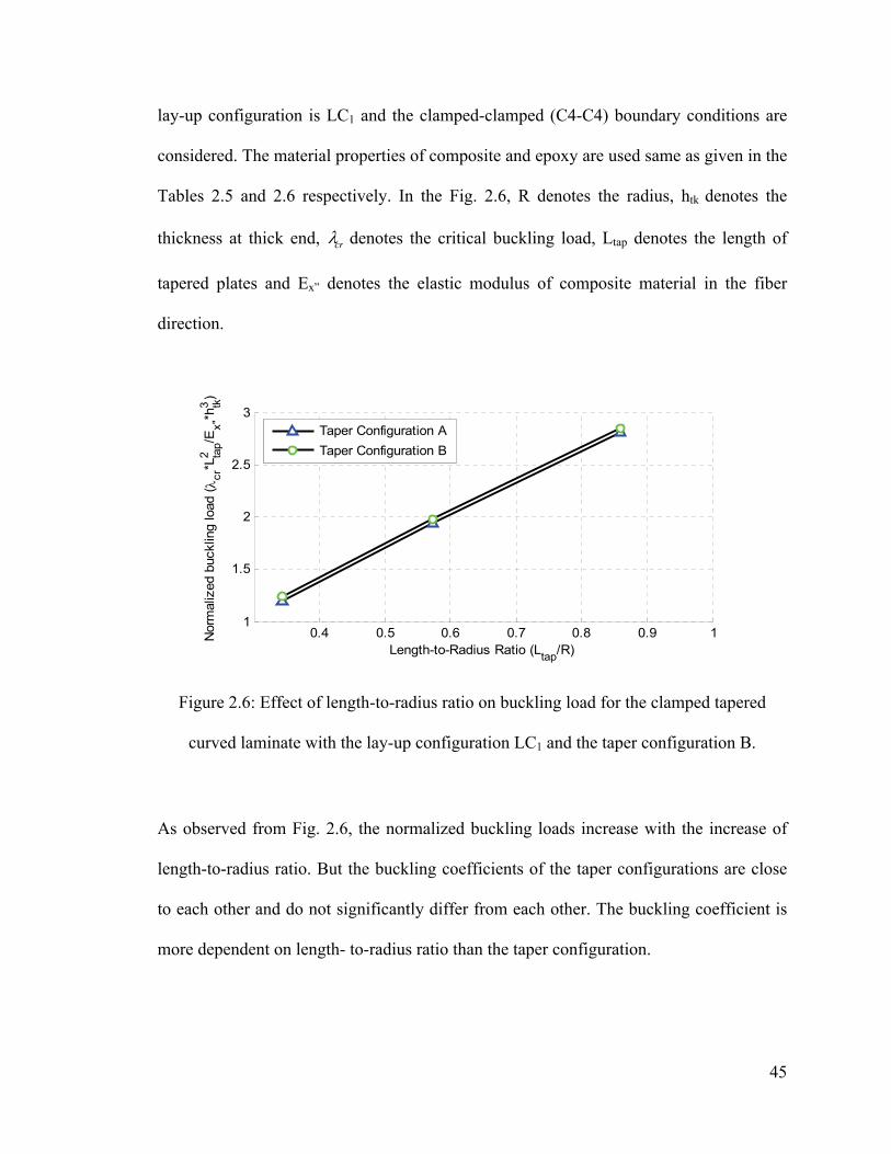
45

lay-up configuration is LC1 and the clamped-clamped (C4-C4) boundary conditions are

considered. The material properties of composite and epoxy are used same as given in the

Tables 2.5 and 2.6 respectively. In the Fig. 2.6, R denotes the radius, htk denotes the

thickness at thick end, crλ denotes the critical buckling load, Ltap denotes the length of

tapered plates and Ex” denotes the elastic modulus of composite material in the fiber

direction.

Figure 2.6: Effect of length-to-radius ratio on buckling load for the clamped tapered

curved laminate with the lay-up configuration LC1 and the taper configuration B.

As observed from Fig. 2.6, the normalized buckling loads increase with the increase of

length-to-radius ratio. But the buckling coefficients of the taper configurations are close

to each other and do not significantly differ from each other. The buckling coefficient is

more dependent on length- to-radius ratio than the taper configuration.

0.4 0.5 0.6 0.7 0.8 0.9 11

1.5

2

2.5

3

Length-to-Radius Ratio (Ltap/R)

Nor

mal

ized

buc

klin

g lo

ad ( λ

cr*L

tap

2/E

x"*h

tk3)

Taper Configuration ATaper Configuration B

46

2.5.2 Buckling Analyses of Hybrid Curved Plates

Laminates with only taper section have been studied in the previous sections and the

hybrid (combinations of tapered and uniform-thickness) sections are taken into account in

the present sub-section of thesis. The tapered part of hybrid plates is modeled using the

configuration B. For the analysis of hybrid configuration three types of lay-up

configurations, namely LC1, LC2 and LC3 given in the Table 2.7 are considered. For the

buckling analysis, total plate length L = 229.2 mm, width b = 114.6 mm and the material

properties of Tables 2.5 and 2.6 are considered. According to the first-ply failure

analysis, the hybrid plates with the above mentioned lay-up configurations will not fail by

first-ply failure before global buckling. Two parameters, namely radius-to-thickness ratio

and boundary conditions are considered to see the influences of these parameters on

buckling load of hybrid curved plates. The results are shown in the following Figs. 2.7

through 2.11.

2.5.2.1 Influence of Lay-Up Configurations

The normalized buckling loads of three lay-up configurations are calculated using Ritz

method as shown in the Figs. 2.7 - 2.8. The buckling loads are calculated for clamped-

clamped (C4-C4) boundary conditions. The buckling load is considered in the Figs. 2.7 -

2.8 to see the influence of the lay-up configurations on R/htk. In these figures, R denotes

the radius, htk denotes the thickness at thick end, crλ denotes the critical buckling load, L

denotes the total length of hybrid plates and Ex” denotes the elastic modulus of composite

material in the fiber direction. From Figs. 2.7 - 2.8, the following observations are made:

a) The lay-up configuration LC2 is the weakest one among all other lay-up

configurations.

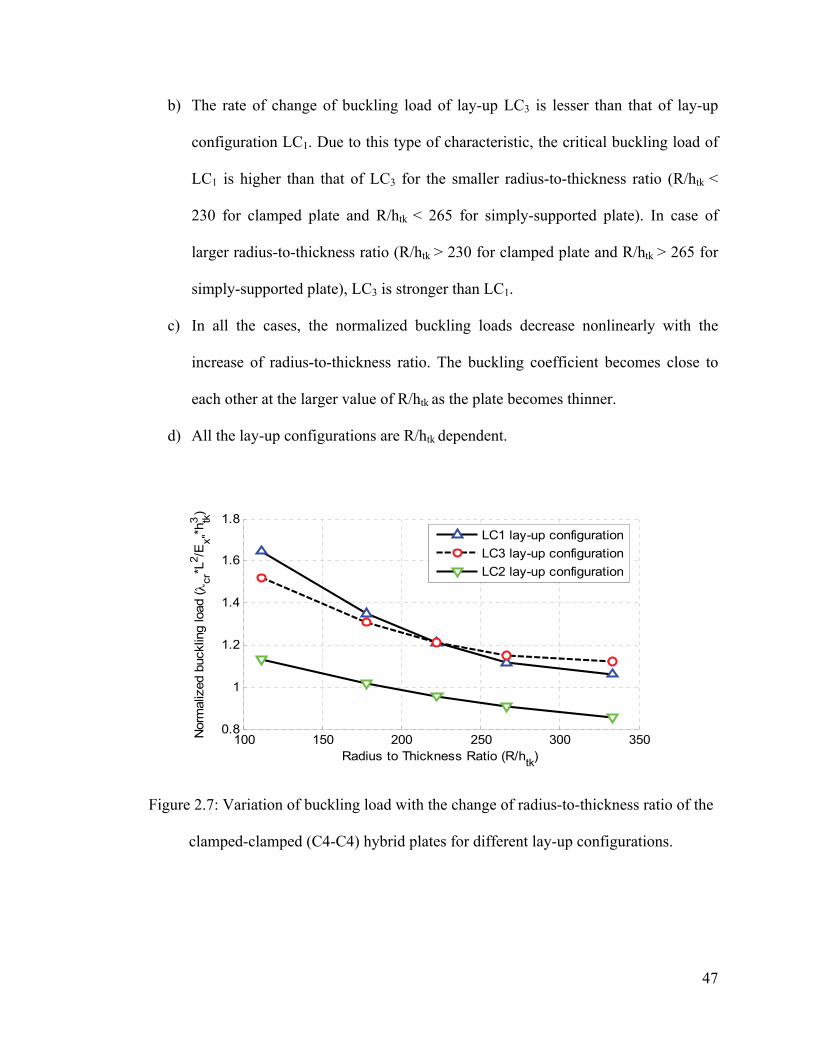
47

b) The rate of change of buckling load of lay-up LC3 is lesser than that of lay-up

configuration LC1. Due to this type of characteristic, the critical buckling load of

LC1 is higher than that of LC3 for the smaller radius-to-thickness ratio (R/htk <

230 for clamped plate and R/htk < 265 for simply-supported plate). In case of

larger radius-to-thickness ratio (R/htk > 230 for clamped plate and R/htk > 265 for

simply-supported plate), LC3 is stronger than LC1.

c) In all the cases, the normalized buckling loads decrease nonlinearly with the

increase of radius-to-thickness ratio. The buckling coefficient becomes close to

each other at the larger value of R/htk as the plate becomes thinner.

d) All the lay-up configurations are R/htk dependent.

Figure 2.7: Variation of buckling load with the change of radius-to-thickness ratio of the

clamped-clamped (C4-C4) hybrid plates for different lay-up configurations.

100 150 200 250 300 3500.8

1

1.2

1.4

1.6

1.8

Radius to Thickness Ratio (R/htk)

Nor

mal

ized

buc

klin

g lo

ad ( λ

cr*L

2 /Ex"

*htk3

)

LC1 lay-up configurationLC3 lay-up configurationLC2 lay-up configuration

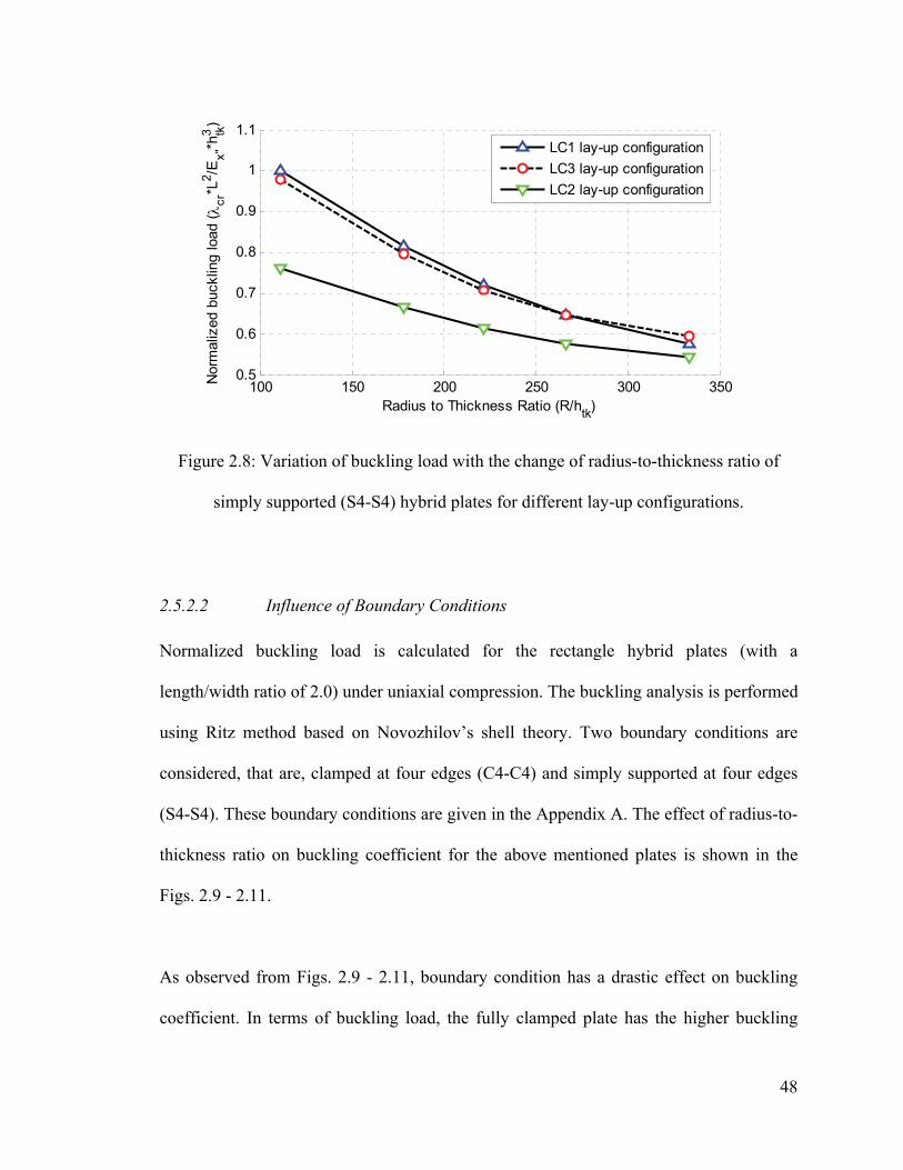
48

Figure 2.8: Variation of buckling load with the change of radius-to-thickness ratio of

simply supported (S4-S4) hybrid plates for different lay-up configurations.

2.5.2.2 Influence of Boundary Conditions

Normalized buckling load is calculated for the rectangle hybrid plates (with a

length/width ratio of 2.0) under uniaxial compression. The buckling analysis is performed

using Ritz method based on Novozhilov’s shell theory. Two boundary conditions are

considered, that are, clamped at four edges (C4-C4) and simply supported at four edges

(S4-S4). These boundary conditions are given in the Appendix A. The effect of radius-to-

thickness ratio on buckling coefficient for the above mentioned plates is shown in the

Figs. 2.9 - 2.11.

As observed from Figs. 2.9 - 2.11, boundary condition has a drastic effect on buckling

coefficient. In terms of buckling load, the fully clamped plate has the higher buckling

100 150 200 250 300 3500.5

0.6

0.7

0.8

0.9

1

1.1


Nor

mal

ized

buc

klin

g lo

ad ( λ

cr*L

2 /Ex"

*htk3

)


49

load than the simply-supported plate. Simply supported plates have more degrees of

freedom than the clamped ones which is the reason for less strength. All the lay-up

configurations are both R/htk and boundary condition dependent.


configuration for different boundary conditions.



100 150 200 250 300 3500

0.5

1

1.5

2


Nor

mal

ized

buc

klin

g lo

ad ( λ

cr*L

2 /Ex"

*htk3

)

C4-C4 Boundary conditionS4-S4 Boundary condition

100 150 200 250 300 3500.4

0.6

0.8

1

1.2


Nor

mal

ized

buc

klin

g lo

ad ( λ

cr*L

2 /Ex"

*htk3

)


50



2.6 CONCLUSIONS

In the present chapter, buckling analysis has been carried out using Ritz method based on

eight well known classical shallow shell theories, namely Donnell’s, Love’s, Mushtari’s,

Timoshenko’s, Vlasov’s, Sander’s, Koiter’s and Novozhilov’s thoeries. Two types of

taper configurations (A and B) and three types of lay-up configurations (LC1, LC2 and

LC3) are considered under uniaxial compressive load. A detailed parametric study of

curved (tapered and hybrid) plates has been conducted that includes the effects of

boundary conditions, stacking sequence, taper configurations, radius, and geometric

parameters of the plates. Among the important conclusions and observations one may list

the following:

100 150 200 250 300 3500.4

0.6

0.8

1

1.2

1.4

1.6

1.8


Nor

mal

ized

buc

klin

g lo

ad ( λ

cr*L

2 /Ex"

*htk3

)


51

a) The buckling results based on different shell theories are close to each other but

the Novozhilov’s theory provides the most conservative result.

b) The moderately thick and tapered curved composite plates may fail by first-ply

failure before global buckling. Therefore the tapered curved plate should be larger

than the corresponding critical size. The critical size depends on both radius and

staking sequence of the curved plates.

c) The tapered flat plate is more flexible than uniform flat plate, but the tapered

curved plate provides a better design option in terms of saving the material without

any compromise of the strength.

d) The normalized buckling load is more dependent on length-to-radius ratio (Ltap/R)

than the taper configuration.

e) The buckling loads of all the lay-up configurations are both radius-to-thickness

ratio (R/htk) and boundary condition dependent.

52

Chapter 3

Ply Failure vs. Global Buckling of Tapered Curved Composite Plates

3.1 INTRODUCTION

In this chapter, approximate analytical solutions are developed using Ritz method for the

global buckling response of tapered curved plates considering uniaxial compression.

Buckling analysis of tapered curved plates is carried out based on six well-established

First-order shear deformation Shell Theories (FST). Various boundary conditions, and

different lay-up and taper configurations are considered. The critical buckling loads

calculated using the Ritz method are compared with that of the existing experimental and

analytical results. The failure strength characteristics and load carrying capability of the

tapered curved plates are studied considering two predominant types of local failures,

which are the first-ply failure and the delamination failure. Based on the failure and

buckling analyses, the critical values of size and shape parameters of the plates such that

they will fail only in global buckling mode are determined. A comprehensive parametric

study is carried out and design guidelines for the tapered curved plates are established

based on this study.

3.2 FORMULATION

To determine the stiffness matrix of a ply in a tapered laminate, three coordinate systems

have been defined: principal material coordinate system ),,( """ zyx , local coordinate system

),,( ''' zyx and global coordinate system (x, y, z). These systems are shown in Fig. 2.1.

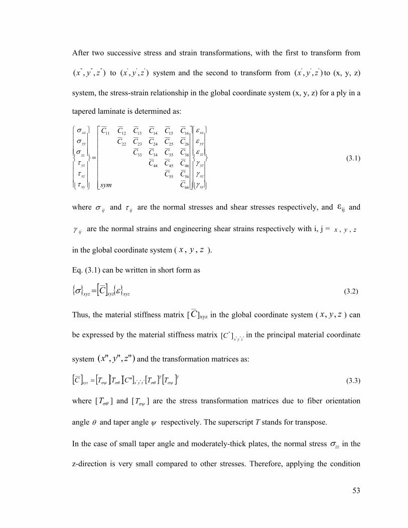
53

After two successive stress and strain transformations, with the first to transform from

),,( """ zyx to ),,( ''' zyx system and the second to transform from ),,( ''' zyx to (x, y, z)

system, the stress-strain relationship in the global coordinate system (x, y, z) for a ply in a

tapered laminate is determined as:

⎪⎪⎪⎪

⎭

⎪⎪⎪⎪

⎬

⎫

⎪⎪⎪⎪

⎩

⎪⎪⎪⎪

⎨

⎧

⎥⎥⎥⎥⎥⎥⎥⎥

⎦

⎤

⎢⎢⎢⎢⎢⎢⎢⎢

⎣

⎡

=

⎪⎪⎪⎪

⎭

⎪⎪⎪⎪

⎬

⎫

⎪⎪⎪⎪

⎩

⎪⎪⎪⎪

⎨

⎧

xy

xz

yz

zz

yy

xx

xy

xz

yz

zz

yy

xx

CsymCCCCCCCCCCCCCCCCCCCC

γγγεεε

τττσσσ

66

5655

464544

36353433

2625242322

161514131211

(3.1)

where ijσ and ijτ are the normal stresses and shear stresses respectively, and ijε and

ijγ are the normal strains and engineering shear strains respectively with i, j = zyx ,,

in the global coordinate system ( zyx ,, ).

Eq. (3.1) can be written in short form as

{ } [ ] { }xyzxyzxyz C εσ = (3.2)

Thus, the material stiffness matrix [C]xyz in the global coordinate system ( zyx ,, ) can

be expressed by the material stiffness matrix """][ "zyxC in the principal material coordinate

system )",","( zyx and the transformation matrices as:

[ ] [ ][ ][ ] [ ] [ ]TTzyxxyz TTCTTC σψσθσθσψ """"= (3.3)

where [ σθT ] and [ σψT ] are the stress transformation matrices due to fiber orientation

angle θ and taper angle ψ respectively. The superscript T stands for transpose.

In the case of small taper angle and moderately-thick plates, the normal stress zzσ in the

z-direction is very small compared to other stresses. Therefore, applying the condition

54

that 0=zzσ in the Eq. (3.1), the corresponding reduced stiffness matrix is calculated and

expressed after rearrangement as:

⎪⎪⎪

⎭

⎪⎪⎪

⎬

⎫

⎪⎪⎪

⎩

⎪⎪⎪

⎨

⎧

⎥⎥⎥⎥⎥⎥

⎦

⎤

⎢⎢⎢⎢⎢⎢

⎣

⎡

=

⎪⎪⎪

⎭

⎪⎪⎪

⎬

⎫

⎪⎪⎪

⎩

⎪⎪⎪

⎨

⎧

xz

yz

xy

yy

xx

xz

yz

xy

yy

xx

QQQQQQQQQQQQQQQQQQQQQQQQQ

γγγεε

τττσσ

5545562515

4544462414

4646662616

2524262212

1514161211

(3.4)

where ;/ 3333 CCCCQ jiijij −= i, j = 1, 2, 4, 5, 6. (3.5)

and ijC is the material stiffness coefficient in the global coordinate system given by the

Eq. (3.3).

The equations for coefficients of matrices [A], [B] and [D] for tapered laminate can be

written as

dzzzQDBAh

hijijijij ),,1(),,( 2

2/

2/∫

−

= i , j = 1,2,4,5,6 (3.6)

The strain-displacement relations corresponding to different shell theories are considered

for the case of small deformations of a curved plate with radius R and written in terms of

the mid-plane displacement field (uo, vo, wo) that refers to the global coordinate system

(x, y, z) as shown in Fig. 2.1. Further, xϕ and yϕ denote the rotations due to shear

deformation. The tracer coefficients c1 and c2 are introduced to express the strain-

displacement relations corresponding to the six different shell theories for shallow

)1/( <<Rhtk curved plate. The strain field can be expressed as:

Toxy

oyy

oxx

Toxz

oyz

oxy

oyy

oxx

Txzyzxyyyxx z ]00[][][ κκκγγγεεγγγεε += (3.7)

55

with

⎪⎪⎪⎪⎪

⎭

⎪⎪⎪⎪⎪

⎬

⎫

⎪⎪⎪⎪⎪

⎩

⎪⎪⎪⎪⎪

⎨

⎧

∂∂

+

−∂∂

+

∂∂

+∂∂

+∂∂

∂∂

=

⎪⎪⎪

⎭

⎪⎪⎪

⎬

⎫

⎪⎪⎪

⎩

⎪⎪⎪

⎨

⎧

xw

Rc

yw

xv

yu

Rw

yv

xu

ox

ooy

oo

oo

o

oxz

oyz

oxy

oyy

oxx

ϕ

νϕγγγεε

2

(3.8)

and

⎪⎪⎪⎪⎪

⎭

⎪⎪⎪⎪⎪

⎬

⎫

⎪⎪⎪⎪⎪

⎩

⎪⎪⎪⎪⎪

⎨

⎧

⎟⎟⎠

⎞⎜⎜⎝

⎛∂∂

−∂∂

+∂

∂+

∂∂

∂

∂∂∂

=

⎪⎪⎪

⎭

⎪⎪⎪

⎬

⎫

⎪⎪⎪

⎩

⎪⎪⎪

⎨

⎧

002

00

1

yu

xv

Rc

xy

y

x

ooyx

y

x

oxy

oyy

oxx

ϕϕ

ϕ

ϕ

κκκ

(3.9)

where the column matrices Txzyzxyyyxx ][ 00000 γγγεε and

Toxy

oyy

oxx ]00[ κκκ are,

respectively, the matrix of mid-plane strains and the matrix of curvatures.

By setting,

i) c1 = c2 = 0, equations that correspond to Donnell’s [108] and Morley’s

[109] shell theories are obtained.

ii) c1 = 0 and c2 = 1, equations that correspond to Love’s [98] and Loo’s

[110] shell theories are obtained.

iii) c1 = 1 and c2 = 1, equations that correspond to Sanders’s [100] and

Koiter’s [101] shell theories are obtained.

56

In the case of shallow shells, the Koiter’s and the Sanders’s shell theories lead to the

same expressions for strains and curvatures. In the present work, shallow tapered

laminated shells are considered. Therefore, these two shell theories are referred to

together as ‘Koiter-Sanders shell theory’.

The force and moment resultants are written using the above mentioned strain field and

the laminate stiffness matrices given in the Eq. (3.6), in the form:

⎪⎪⎪⎪⎪⎪

⎭

⎪⎪⎪⎪⎪⎪

⎬

⎫

⎪⎪⎪⎪⎪⎪

⎩

⎪⎪⎪⎪⎪⎪

⎨

⎧

⎥⎥⎥⎥⎥⎥⎥⎥⎥⎥⎥⎥⎥

⎦

⎤

⎢⎢⎢⎢⎢⎢⎢⎢⎢⎢⎢⎢⎢

⎣

⎡

⎟⎟⎠

⎞⎜⎜⎝

⎛⎟⎟⎠

⎞⎜⎜⎝

⎛

⎟⎟⎟⎟

⎠

⎞

⎜⎜⎜⎜

⎝

⎛

⎟⎟⎟

⎠

⎞

⎜⎜⎜

⎝

⎛

=

⎪⎪⎪⎪⎪

⎭

⎪⎪⎪⎪⎪

⎬

⎫

⎪⎪⎪⎪⎪

⎩

⎪⎪⎪⎪⎪

⎨

⎧

oxz

oyz

oxy

oyy

oxx

oxy

oyy

oxx

xz

yz

xy

yy

xx

xy

yy

xx

AAAA

SBBBBBB

AAAAAA

S

BBBBBB

SDDDDDDDDD

BBBBBBBBB

AAAAAA

SBBBBBBBBB

AAAAAAAAA

QQMMMNNN

γγκκκγεε

5545

45443

562515

462414

562515

4624142

5646

2524

1514

1

662616

262212

161211

662616

262212

161211

5646

2524

1514

1

662616

262212

161211

662616

262212

161211

(3.10a)

The Eq. (3.10a) can be written in a short form as:

}]{[ ' εEQMN

=⎪⎭

⎪⎬

⎫

⎪⎩

⎪⎨

⎧ (3.10b)

In the Eq. (3.10a) S1, S2 and S3 are the Shear Correction (SC) factors. For uniform plate

the coefficients S1 and S2 are set to be equal to zero but the coefficient S3 is non-zero.

Moreover, the value of S3 is considered to be 5/6 for uniform plate. For a tapered plate

the coefficients S1, S2 and S3 will have non-zero values. There is no experimental or

analytical work that is currently available as to what values of S1, S2 and S3 are

appropriate for tapered laminated plates. Considering this, in the present work, all

possible combinations of these SC factors (S1, S2 and S3) are considered and

corresponding analyses are conducted. The number of permutations of three SC factors

57

by taking the two numerical values (1 and 5/6) at a time is to be 6. Accordingly, the

following six sets of SC factors are considered in the buckling analysis and

corresponding critical buckling loads are calculated.

S1=1, S2=1, S3=1 (3.11a)

S1=1, S2=1, S3=5/6 (3.11b)

S1=1, S2 =5/6, S3 =5/6 (3.11c)

S1=5/6, S2=5/6, S3 =5/6 (3.11d)

S1=5/6, S2 =5/6, S3 =1 (3.11e)

S1=5/6, S2=1, S3 =1 (3.11f)

The set of SC factors that corresponds to the most conservative value of critical buckling

loads is determined using the results of the analyses. This particular set of values is used

futher onwards throughout the present work. For this purpose, a tapered plate with

configuration B and having 36 layers at the thick end with [0/90]9s lay-up and 12 layers at

the thin end with [0/90]3s lay-up, that is subjected to uni-axial end compressive loading

has been analyzed using Ritz method. The plate is clamped at four edges (C4-C4) and the

boundary conditions represented as C4 are given in the Appendix B. The dimensions of

the square plate are (see Fig. 1.4): various values of the side length of the plate in the

range of from 85.94 mm to 171.90 mm are considered, plate thickness at thick end htk =

4.5 mm and radius R = 500 mm. The material properties of the composite ply and epoxy

are the same as given in Tables 2.5 and 2.6 respectively. The critical buckling load using

six shear correction factors is shown in the Fig. 3.1 at the end of this section.

The strain energy of a tapered plate is written in Cartesian co-ordinates as follows:

58

[ ]( ) dxdyEb L

Ttap

∫ ∫=∏0 0

' }{}{21 εε (3.12)

where Txzyzxyyyxxxyyyxx ][}{ 00000000 γγκκκγεεε = (3.13)

and [E’] is the stiffness matrix given in Eq. (3.10b).

The potential energy corresponding to the uni-axial end compression λ is

dxdyx

wxv

xu

Wb L

oootap

∫ ∫⎪⎭

⎪⎬⎫

⎪⎩

⎪⎨⎧

⎥⎥⎦

⎤

⎢⎢⎣

⎡⎟⎠

⎞⎜⎝

⎛∂∂

+⎟⎠

⎞⎜⎝

⎛∂∂

+∂∂

−=0 0

22

21λ (3.14)

The approximate solutions for the displacement fields and rotations are expressed as a

double series:

∑∑= =

=M

m

N

nnmmno yUxUUyxu

1 1)()(),(

(3.15)

∑∑= =

=M

m

N

nnmmno yVxVVyxv

1 1)()(),(

(3.16)

∑∑= =

=M

m

N

nnmmno yWxWWyxw

1 1)()(),(

(3.17)

∑∑= =

=M

m

N

nnmmnx yXxXXyx

1 1)()(),(ϕ

(3.18)

∑∑= =

=M

m

N

nnmmny yYxYYyx

1 1)()(),(ϕ

(3.19)

The functions Um(x), Un(y), Vm(x), Vn(y), Wm(x), Wn(y), Xm(x), Xn(y), Ym(x) and Yn(y)

are so chosen as to satisfy the boundary conditions which are given in the Appendix B

and the coefficients Umn, Vmn, Wmn , Xmn and Ymn are determined by the following

stationary conditions:

59

mnmn UW

U ∂∂

=∂∏∂ (3.20)

mnmn VW

V ∂∂

=∂∏∂ (3.21)

mnmn WW

W ∂∂

=∂

∏∂ (3.22)

mnmn XW

X ∂∂

=∂

∏∂ (3.23)

mnmn YW

Y ∂∂

=∂∏∂ (3.24)

where, ∏ and W are given by the Eqs. (3.12) and (3.14) respectively.

Using the Eqs. (3.20) through (3.24) the following matrix equation is obtained:

[ ] [ ] [ ] [ ] [ ][ ] [ ] [ ] [ ] [ ][ ] [ ] [ ] [ ] [ ][ ] [ ] [ ] [ ] [ ][ ] [ ] [ ] [ ] [ ] ⎪

⎪⎪

⎭

⎪⎪⎪

⎬

⎫

⎪⎪⎪

⎩

⎪⎪⎪

⎨

⎧

⎥⎥⎥⎥⎥⎥

⎦

⎤

⎢⎢⎢⎢⎢⎢

⎣

⎡

−=

⎪⎪⎪

⎭

⎪⎪⎪

⎬

⎫

⎪⎪⎪

⎩

⎪⎪⎪

⎨

⎧

⎥⎥⎥⎥⎥⎥

⎦

⎤

⎢⎢⎢⎢⎢⎢

⎣

⎡

IJ

IJ

IJ

IJ

IJ

IJ

IJ

IJ

IJ

IJ

IJ

IJ

IJIJIJIJIJ

IJIJIJIJIJ

IJIJIJIJIJ

IJIJIJIJIJ

IJIJIJIJIJ

YXWVU

GG

YXWVU

LLLLLLLLLLLLLLLLLLLLLLLLL

]0[]0[]0[]0[]0[]0[]0[]0[]0[]0[]0[]0[][]0[]0[]0[]0[]0[][]0[]0[]0[]0[]0[]0[

33

22

5545352515

4544342414

3534332313

2524232212

1514131211

λ

(3.25)

Further details about the matrices ],[],[],[],[ 33221211IJIJIJIJ GGLL and so on are given in the

Appendix B. The eigenvalues λ are the values of buckling loads. The following indicial

expressions were introduced [105] and used in the Eq. (3.25):

nMmI +−= )1( and jNiJ +−= )1( (3.26)

where Mmi ......2,1, = and Nnj ......2,1, = .

Eq. (3.25) can be written in a short form:

0][][ '' =+ ZK λ (3.27)

60

where [K’] and [Z’] are the stiffness matrix and geometric stiffness matrix respectively of

the tapered plate. Eq. (3.27) is solved using MATLAB® as an eigenvalue problem. The

smallest value of λ is the critical buckling load, crλ .

The critical buckling loads of taper configuration B corresponding to various taper angles

are plotted in the Fig. 3.1. It can be seen from Fig. 3.1 that the set (S1=1, S2=5/6, S3=5/6)

given in the Eq. (3.11c) is the most conservative one in terms of critical buckling load.

This set of shear correction factors will be used further onwards in the present work.


the laminate with the taper configuration B based on Koiter-Sanders shell theory.

3.3 VALIDATION

The commercial software ANSYS® has been chosen to model the curved composite

plates to compare the buckling loads obtained using Ritz method based on FST. Element

SHELL99 is used for the analyses using ANSYS®. SHELL99 is an 8-node, 3-D shell

element with six degrees of freedom (three translations and three rotations) at each node.

It is designed based on the degenerated solid approach with shear deformation effect and

0.5 0.55 0.6 0.65 0.7 0.75 0.8 0.85 0.9 0.95 14

5

6

7

8

9

10x 105

Taper angle (ψo)

Crit

ical

buc

klin

g lo

ad (N

/m)

S1=1, S2=1, S3=1S1=1, S2=1, S3=5/6S1=1, S2=5/6, S3=5/6S1=5/6, S2=5/6, S3=5/6S1=5/6, S2=5/6, S3=1S1=5/6, S2=1, S3=1

61

to model thin to moderately-thick plate and shell structures with a side-to-thickness ratio

of roughly 10 or greater. The tapered curved plates are meshed by using eighty-one

elements which are shown by numbering in the Fig. 2.2.

To the authors’ knowledge, no results are available yet in the literature on the buckling

loads of the tapered curved composite plates under the action of uni-axial compression.

Therefore the comparison with the existing works could not be made. However, in order

to validate the formulation and analysis, first, the taper angle is set to be zero, and the

resulting uniform-thickness laminates have been analyzed and the results have been

compared with that available in the literature for the uniform-thickness laminates [107].

For this reason, a uniform-thickness cylindrical panel made of T300/5208 graphite/epoxy

material having the mechanical properties of Ex” = 141.34 GPa (20.5 x106 psi), Ey” = 8.96

GPa (1.3 x106 psi), Gx”y” = 5.17 GPa (0.75 x106 psi) and υ = 0.335 are considered. The

plate is clamped (C3) in transverse direction and simply-supported (S3) in longitudinal

direction. The boundary conditions C3 and S3 are given in the Appendix B. The

dimensions of the plate are taken to be: length L = 0.3048 m (12 inches), cord 'b =

0.3048 m, radius R = 0.3048 m, thickness h = 1.016x10-03 m (0.04 inches). Becker [107]

has conducted the bifurcation (obtained from eigenvalue solution) buckling analysis of

this curved plate using STAGS computer code. In the present study, the buckling analysis

is carried out using Ritz method based on various shell theories and the results are

compared with that given in the work of Becker [107]. The buckling load is also obtained

using ANSYS®. The normalized buckling load is given in the Table 3.1 wherein crλ

denotes the critical buckling load.

62

As can be observed from the Table 3.1, the results obtained in the present work are in

good agreement with the theoretical buckling load given in the reference work. The

present results as well as the theoretical results given in Becker [107] are higher than the

experimental result. According to Ref. [107], the bifurcation buckling load may be 23 to

45 percent higher than the experimental result for the critical buckling load. The results

obtained based on different shell theories are somewhat close to each other but the

Koiter-Sanders shell theory provides the most conservative result. The result obtained

using ANSYS® overestimates the critical buckling load. Therefore in the present study,

the Koiter-Sanders shell theory is used to calculate the buckling load using Ritz method.

Table 3.1: Comparison of critical buckling loads for the uniform-thickness cylindrical

plate

Laminate Configuration

Becker [107] )/()( 3"

2 hEL xcrλ Present )/()( 3"

2 hEL xcrλ

Exp. Theory (Bifurcation)

Donnell, Morley

Koiter- Sanders Love, Loo ANSYS®

[90/0]2s 24.50 33.30 34.84 34.70 34.75 37.34

Next, a tapered plate with only two (one above and corresponding one below the mid

plane) internally-dropped plies has been analyzed using Ritz method based on Koiter-

Sanders theory. The plate has configuration [90/0]2s at thick end and [90/0/90]s at thin

end. The material properties of the ply and the dimensions of the plate are the same as

that mentioned before for the uniform-thickness cylindrical plate (Ref. [107]). The

clamped-simply supported (C3-S3) boundary conditions are considered as in the previous

case. The results obtained for critical buckling load are compared with that of two

63

uniform-thickness composite plates with lay-up configurations [90/0]2s and [90/0/90]s,

respectively. The critical buckling loads for these three laminates under uni-axial end

compressive load are given in Table 3.2. As can be observed, the result for the tapered

laminate is between that of the 8-layers uniform-thickness laminate and that of the 6-

layers uniform-thickness laminate.


Plate Critical Buckling Load (x 104 N/m) 8-Layers Uniform Plate [90/0]2s

5.5366

Tapered Plate [90/0]2s - [90/0/90]s

4.0094

6-Layers Uniform Plate [90/0/90]s

2.9074

3.4 FIRST-PLY FAILURE ANALYSIS

The strength in compression of the tapered curved plate is investigated considering first-

ply failure. This type of failure analysis is considered in the present work to determine

whether any layer has failed (locally) due to compressive loading before the laminate as a

whole fails on global buckling. First-ply failure analysis is carried out using ANSYS®

based on the 3-D version of Tsai-Wu failure criterion given in the ANSYS® reference

manual. The first-ply failure refers to the first instant at which any layer or more than one

layer fails at the same load. The same criterion is applied for both the composite ply and

the resin pocket. For this purpose, the resin pocket is considered (imagined) to be made

up of layers of isotropic resin material. Material properties of composite ply and epoxy

resin are given in the Tables 2.5 and 2.6 respectively.

64

Four square-shaped tapered composite plates of different sizes with taper configuration B

(Fig. 1.4) and made of NCT/301 graphite-epoxy composite material are considered. The

lay-up configuration for all the plates is [0/90]9s at the thick end and [0/90]3s at the thin

end. This laminate is referred to as the laminate with lay-up configuration LC1 in the

Table 2.7 and further onwards. The side length of each of the square plates is as given in

the Table 3.3, plate thickness at the thick end (htk) is 4.5 mm and the radius (R) of the

plates is 500 mm. The clamped-clamped (C4-C4) boundary conditions as described in the

Appendix B are considered. The results of first-ply failure analysis are summarized in the

Table 3.3 along with the results of buckling analysis.

In the Table 3.3, the first-ply failure loads are compared with the buckling loads. As can

be seen from this table, the tapered curved plates corresponding to taper angles of 0.75

and 1.0 degrees will fail by first-ply failure before the global buckling. On the other hand,

the plates corresponding to taper angles of 0.1 and 0.50 degrees will not fail by first-ply

failure even at the state of global buckling. Therefore, the maximum plate size should be

corresponding to a taper angle of 0.53 degree and the critical length-to-height ratio (Ltap /

htk) is to be 36. The failed layers numbered 2 and 3 respectively are the second layer and

the third layer from the bottom surface of the laminate at the thick end of the plate. All

the tapered curved plates failed at the thick end where the numbers of plies above or

below the resin pockets are at minimum.

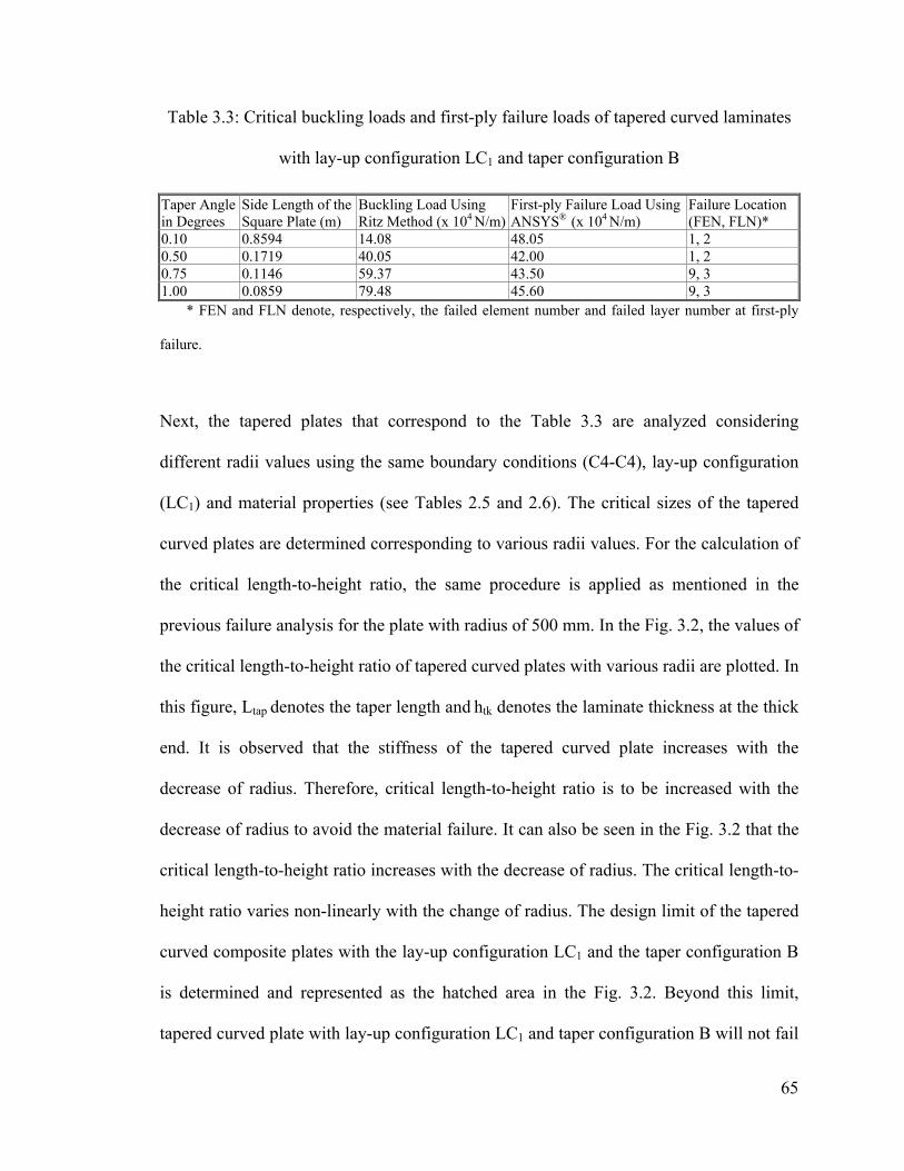
65

Table 3.3: Critical buckling loads and first-ply failure loads of tapered curved laminates

with lay-up configuration LC1 and taper configuration B

Taper Angle in Degrees


Buckling Load Using Ritz Method (x 104 N/m)

First-ply Failure Load Using ANSYS® (x 104 N/m)


0.10 0.8594 14.08 48.05 1, 2 0.50 0.1719 40.05 42.00 1, 2 0.75 0.1146 59.37 43.50 9, 3 1.00 0.0859 79.48 45.60 9, 3

* FEN and FLN denote, respectively, the failed element number and failed layer number at first-ply

failure.

Next, the tapered plates that correspond to the Table 3.3 are analyzed considering

different radii values using the same boundary conditions (C4-C4), lay-up configuration

(LC1) and material properties (see Tables 2.5 and 2.6). The critical sizes of the tapered

curved plates are determined corresponding to various radii values. For the calculation of

the critical length-to-height ratio, the same procedure is applied as mentioned in the

previous failure analysis for the plate with radius of 500 mm. In the Fig. 3.2, the values of

the critical length-to-height ratio of tapered curved plates with various radii are plotted. In

this figure, Ltap denotes the taper length and htk denotes the laminate thickness at the thick

end. It is observed that the stiffness of the tapered curved plate increases with the

decrease of radius. Therefore, critical length-to-height ratio is to be increased with the

decrease of radius to avoid the material failure. It can also be seen in the Fig. 3.2 that the

critical length-to-height ratio increases with the decrease of radius. The critical length-to-

height ratio varies non-linearly with the change of radius. The design limit of the tapered

curved composite plates with the lay-up configuration LC1 and the taper configuration B

is determined and represented as the hatched area in the Fig. 3.2. Beyond this limit,

tapered curved plate with lay-up configuration LC1 and taper configuration B will not fail

66

by first-ply failure before global buckling. Similar type of effect is also considered in the

Fig. 2.3, where the critical length-to-height ratio (Ltap / htk) is to be 38.9 corresponds to

taper angle of 0.49 degree.

Figure 3.2: The relation between the critical length-to-height ratio and the radius of the

tapered curved composite plate with the lay-up configuration LC1 and the taper

configuration B.

3.5 DELAMINATION FAILURE ANALYSIS

The initiation of delamination, if any, is dictated by the transverse interlaminar stresses

developed under compressive load. In ANSYS®, interlaminar transverse shear stresses in

shell element are calculated based on the assumption that no shear is carried at the top

and bottom surfaces of the element. These interlaminar shear stresses are only computed

in the interior of the element and are computed using equilibrium requirements.

Delamination at any interface between any two adjacent layers is said to have occurred

16 18 20 22 24 26 28 30 32 34 360.5

0.6

0.7

0.8

0.9

1

1.1

1.2

1.3

1.4

1.5

Critical Length-to-Height Ratio (Ltap/htk)crt

Rad

ius

(m)

67

when any of the transverse stress components in any of the two layers adjacent to the

interface becomes equal to or greater than its corresponding allowable strength. Four

square tapered composite plates of different sizes with taper configuration B and made of

NCT/301 graphite-epoxy composite material are considered. The lay-up is [0/90]9s at the

thick end and [0/90]3s at the thin end which together is defined as lay-up configuration

LC1 in the Table 2.7. The material properties of the composite ply and epoxy material are

given in the Tables 2.5 and 2.6 respectively. The side length of the square plate varies

from 85.9 to 859.4 mm, plate thickness at the thick end (htk) is 4.5 mm and radius (R) of

the plates is 500 mm. The clamped-clamped (C4-C4) boundary conditions described in

the Appendix B is considered. The averaged maximum interlaminer shear stresses are

calculated in the present work at the state of first-ply failure load or critical buckling load

(considering the larger one) and the corresponding locations are tabulated in the Table

3.4. The failed layers numbered 5 and 13 are, respectively, below and above the large

resin pocket at the thin end.

Table 3.4: Averaged maximum interlaminar shear stress of clamped-clamped (C4-C4)

tapered curved laminate with lay-up configuration LC1 and taper configuration B


Side Length of Square Plate (m)

Compressive End Load (x 104 N/m)

Maximum Interlaminar Shear Stress, (MPa)

Location (EN, LLN)** Remark

0.10 0.8594 48.05 1.01 63, 5 No Initiation of Delamination

0.50 0.1719 42.00 0.57 63, 5 0.75 0.1146 59.37 0.99 55, 13 1.00 0.0859 79.48 1.25 63, 5

** EN and LLN denote, respectively, the element number and lower layer number adjacent to the interface

where the interlaminer shear stress is maximum.

68

It is observed from the Table 3.4 that no initiation of delamination takes place for the

taper configuration B and lay-up configuration LC1 at the states of first-ply failure or

global buckling. This is so because the maximum interlaminer shear stress in both the

cases is less than the corresponding allowable shear strength of the composite material.

As an alternative approach, thin resin layers of thickness 0.0125 mm each are considered

above the top resin pockets and below the bottom resin pockets as shown by the thick

lines (thick lines are used to show these layers more clearly) in the Fig. 3.3; these thin

resin plies are defined as ‘resin-rich layers’. The longitudinal cross-section across the

middle of curved laminate is considered. The thin resin-rich layers having thickness of

one-tenth of a composite ply are taken into account in the analysis and transverse

interlaminar normal and shear stresses developed at the locations of the ply drop-off are

calculated to determine the stress states at these locations. The plate with a taper angle of

1 degree corresponding to the data given in the Table 3.4 is investigated using the same

boundary conditions (C4-C4), ply-configuration (LC1) and material properties (see

Tables 2.5 and 2.6). The stresses are calculated under the compressive load of 79.48x104

N/m which is the critical buckling load corresponding to taper angle of 1 degree. The

stresses at the top thin ‘resin-rich layers’ in the global coordinate directions (x,y,z) are

plotted in the Fig. 3.4.

69

Figure 3.3: Longitudinal cross-section of taper configuration B with thin resin-rich layers.

Figure 3.4: The stresses at the top ‘resin-rich layers’ with lay-up configuration LC1 and

taper configuration B for the taper angle of 1 degree.

From the stress distributions in ‘resin-rich layers’ shown in the Fig. 3.4, it is observed

that significant normal and transverse stresses are present at these locations. These

stresses are localized close to the region near the ply drops which are the probable

locations for the initiation of delamination. In the Table 3.4, only the locations of

maximum interlaminer stresses are identified but the present alternate approach is

required to observe the distribution of these stresses along longitudinal direction. The

drop in the normal stress zzσ at each ply drop-off location is relatively higher than that in

the interlaminar shear stresses. In addition, the drop in zzσ at the ply drop-off that is

close to the thin end is relatively the largest. It is to mention that the plate analyzed in

0 0.01 0.02 0.03 0.04 0.05 0.06 0.07 0.08 0.09-15

-10

-5

0

5x 106 Stresses at the top resin-rich layers

x (m)

Stre

ss (P

a)

shear stress (τxz)normal stress (σzz)shear stress (τyz)

70

Fig. 3.4 will fail by first-ply failure load before global buckling as shown in Table 3.3.

This may be the cause of the trace of normal stress zzσ . A similar stress distribution has

been observed at the bottom thin resin-rich layers.


In the parametric study three types of longitudinal cross-sections of the curved plates are

considered, that are, taper configurations A and B, and a hybrid configuration as shown

in the Fig. 1.4. The Ritz solution is obtained based on Koiter-Sanders shell theory. The

same material properties of composite ply and epoxy that are given in the Tables 2.5 and

2.6 respectively are used. The sizes of the plates are so chosen that the plates will not fail

by first-ply failure before global buckling.

3.6.1 Buckling Analysis of Tapered Curved Plates

Tapered models shown in the Fig. 1.4 are considered with 36 and 12 plies at thick and


end is [0/90]9s, and that of the thin end is [0/90]3s (this lay-up configuration is defined

before as LC1). In the analyses of taper configurations, the thickness at the thick end htk is

set to be 4.5 mm and the radius of curved plate R is set to be 500 mm. For all taper

configurations only LC1 lay-up configuration with the boundary conditions of clamped at

all four edges (C4-C4) are considered. The effects of various parameters, namely the ply

drop-off parameters, taper angle and length-to-radius ratio on the critical buckling load of

the tapered curved plates are investigated. The results are shown in the following Figs.

3.5 through 3.7.

71


The effect of ply drop-off on critical buckling load is shown in the Fig. 3.5. To


corresponding to a taper angle of 0.1 degree. The thickness at the thick end is not

changed and the taper angle is varied with the corresponding increase in the number of

drop-off plies. The plate can be considered as a uniform-thickness plate when the

number of ply drop-off is set to zero and the taper configuration A is obtained by

dropping off twenty-four plies. The plates are clamped (C4-C4) at the four edges and the

lay-up configuration is LC1. In the Fig. 3.5, crλ denotes the critical buckling load.

From the Fig. 3.5, it is observed that the uniform-thickness curved plate is many times

stiffer than the uniform-thickness flat plate in terms of buckling behavior. It is also

observed that the tapered flat plate is less stiff than uniform flat plate. However, this

strength reduction can be compensated for if the tapered plate is made into a curved one.

Buckling loads of flat and curved plates vary linearly with the number of ply drop-offs. It

can be concluded from the Fig. 3.5 that the tapered curved plate provides a better design

option in terms of saving the material without any compromise of the strength.

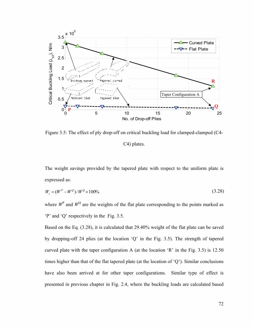
72

Figure 3.5: The effect of ply drop-off on critical buckling load for clamped-clamped (C4-

C4) plates.

The weight savings provided by the tapered plate with respect to the uniform plate is

expressed as:

%100/)( ×−= QQPs WWWW (3.28)

where WP and WQ are the weights of the flat plate corresponding to the points marked as

‘P’ and ‘Q’ respectively in the Fig. 3.5.

Based on the Eq. (3.28), it is calculated that 29.40% weight of the flat plate can be saved

by dropping-off 24 plies (at the location ‘Q’ in the Fig. 3.5). The strength of tapered

curved plate with the taper configuration A (at the location ‘R’ in the Fig. 3.5) is 12.50

times higher than that of the flat tapered plate (at the location of ‘Q’). Similar conclusions

have also been arrived at for other taper configurations. Similar type of effect is

presented in previous chapter in Fig. 2.4, where the buckling loads are calculated based

0 5 10 15 20 250

0.5

1

1.5

2

2.5

3

3.5x 105

No. of Drop-off Plies

Crit

ical

Buc

klin

g Lo

ad ( λ

cr),

N/m

Curved PlateFlat Plate


P

R

Q

73

on classical shell theory. In Fig. 2.4, the buckling loads for both of the uniform and

curved plates are 1.24 % higher than that of the present FST-based solution.


The effect of the taper angle of the plate on the critical buckling load is determined using

Ritz method based on First-order shear deformation Shell Theory (FST). The results are

also compared with that obtained using Ritz method based on Classical Shell Theory

(CST) given in the Refs. [111-112] and using Finite Element Method (FEM) given in the

Ref. [113]. The size of the plate is decreased with the increase of taper angle while

keeping the thickness of the thick section unchanged. The maximum and minimum edge

lengths of the tapered curved square plates are, respectively, 859.4 mm corresponding to

a taper angle of 0.1 degree and 171.9 mm corresponding to a taper angle of 0.5 degree.

The comparison of critical buckling loads is shown in the Fig. 3.6 wherein crλ denotes

the critical buckling load.

As can be observed, in all the three cases the critical buckling load increases as the taper

angle is increased, because the plates become shorter (without any change in the

thickness of the thick section) with the increase of taper angle. The buckling loads given

in the Refs. [112] and [113] are, respectively, calculated using Ritz method based on

Novozhilov’s Classical Shell Theory (CST) and the nine-node Lagrange finite element

based on First-order shear deformation Shell Theory (FST). In the case of buckling

analysis based on the present FST based Ritz solution has more degrees of freedom

compared to other two solutions (CST based Ritz solution and FST based FEM solution).

For this reason, the buckling loads calculated using the present FST based Ritz solution

74

can be considered as the most conservative ones. At lower values of taper angle, the

critical buckling loads calculated using the three different approaches do not vary

significantly. On the other hand, at higher values of taper angle, the values of the critical

buckling loads differ relatively much. Therefore it would be better to use the FST based

Ritz solution for the thick and short plates. It can also be observed that in all the three

cases, the critical buckling load varies nonlinearly with the variation of taper angle.

Figure 3.6: Effect of taper angle on the critical buckling load of clamped-clamped (C4-

C4) tapered curved plate with lay-up configuration LC1 and taper configuration B.


The buckling loads of plates of different sizes are calculated using the present FST based

Ritz solution and are compared with the buckling loads obtained using ANSYS®. The

lay-up configuration is LC1 and the clamped-clamped (C4-C4) boundary conditions are

considered. The material properties used for composite ply and epoxy are the same as

0.1 0.15 0.2 0.25 0.3 0.35 0.4 0.45 0.51

2

3

4

5x 105

Taper angle (ψo)

Crit

ical

buc

klin

g lo

ad ( λ

cr),

N/m CST (Ritz) [111-112]

FST (FEM) [113]FST (Ritz,Koiter-Sanders)

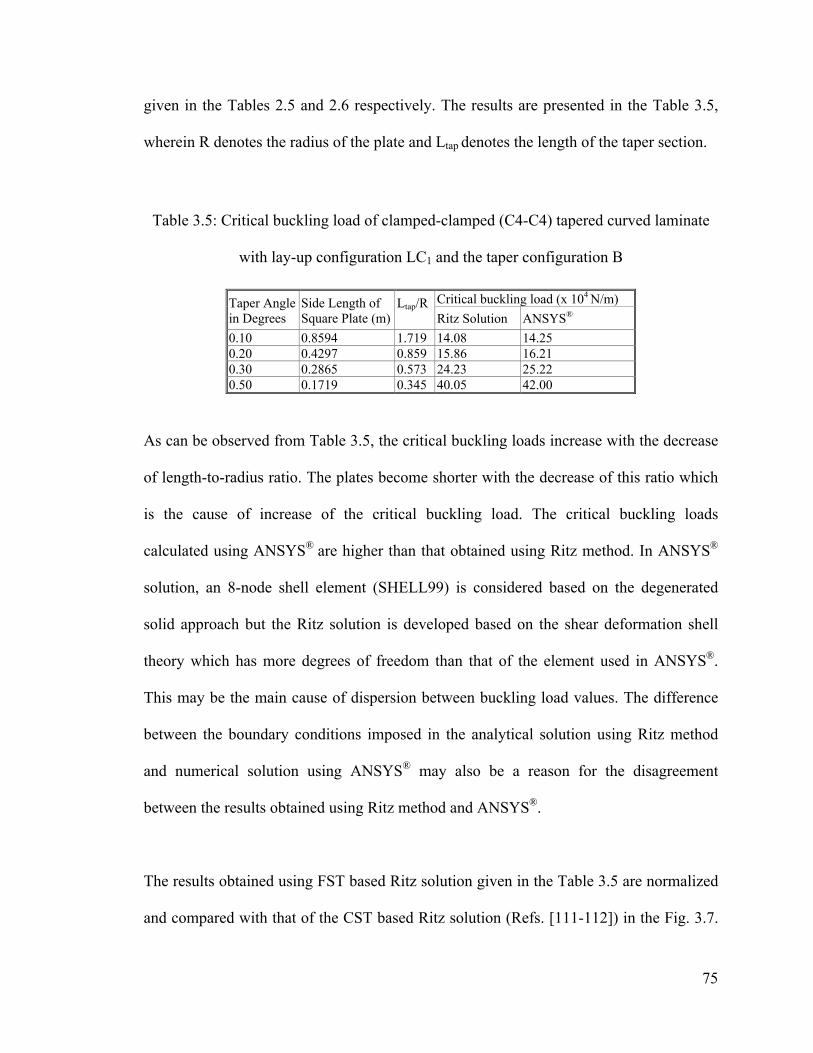
75

given in the Tables 2.5 and 2.6 respectively. The results are presented in the Table 3.5,

wherein R denotes the radius of the plate and Ltap denotes the length of the taper section.

Table 3.5: Critical buckling load of clamped-clamped (C4-C4) tapered curved laminate

with lay-up configuration LC1 and the taper configuration B


Side Length of Square Plate (m)

Ltap/R

Critical buckling load (x 104 N/m) Ritz Solution ANSYS®

0.10 0.8594 1.719 14.08 14.25 0.20 0.4297 0.859 15.86 16.21 0.30 0.2865 0.573 24.23 25.22 0.50 0.1719 0.345 40.05 42.00

As can be observed from Table 3.5, the critical buckling loads increase with the decrease

of length-to-radius ratio. The plates become shorter with the decrease of this ratio which

is the cause of increase of the critical buckling load. The critical buckling loads

calculated using ANSYS® are higher than that obtained using Ritz method. In ANSYS®

solution, an 8-node shell element (SHELL99) is considered based on the degenerated

solid approach but the Ritz solution is developed based on the shear deformation shell

theory which has more degrees of freedom than that of the element used in ANSYS®.

This may be the main cause of dispersion between buckling load values. The difference

between the boundary conditions imposed in the analytical solution using Ritz method

and numerical solution using ANSYS® may also be a reason for the disagreement

between the results obtained using Ritz method and ANSYS®.

The results obtained using FST based Ritz solution given in the Table 3.5 are normalized

and compared with that of the CST based Ritz solution (Refs. [111-112]) in the Fig. 3.7.

76

In this figure, R denotes the radius, htk denotes the thickness at the thick end, crλ denotes

the critical buckling load, Ltap denotes the length of taper section and Ex” denotes the

elastic modulus of composite ply material in the longitudinal direction.


clamped tapered curved plates with the lay-up configuration LC1 and the taper

configuration B.

The normalized buckling load called herein as the buckling coefficient decreases with the

decrease of length-to-radius ratio of the tapered curved plate. The buckling coefficient

calculated based on FST deviates away from that of CST with the increase of thickness of

the plate as the rotations ( xϕ and yϕ ) due to shear deformation play an important role.

The difference between the critical buckling loads calculated using FST and CST is close

to 10% corresponding to the moderately-long plate (Ltap/R = 0.35). This difference

increases with the decrease of length-to-radius ratio (Ltap/R) as the plate becomes shorter.

0.2 0.3 0.4 0.5 0.6 0.7 0.8 0.9 10.5

1

1.5

2

2.5

3

Length-to-Radius Ratio (Ltap/R)

Nor

mal

ized

Buc

klin

g Lo

ad ( λ

cr*L

tap

2/E

x"*h

tk3)

CST (Ritz) [Refs.111-112]

FST (Ritz, Koiter-Sander)

77

3.6.2 Buckling Analysis of Hybrid Curved plates

Laminates with only taper configuration have been studied in the previous sections of the

present chapter. The hybrid configuration (consisting of both tapered and uniform-

thickness sections) is taken into account in the present sub-section. The tapered section of

hybrid plate is considered to have the taper configuration B. For the analysis of hybrid

configuration three types of lay-up configurations, namely LC1, LC2 and LC3 given in the

Table 2.7 are considered. For the buckling analysis, the total plate length L = 229.2 mm,

width b = 114.6 mm and the material properties given in the Tables 2.5 and 2.6 are

considered. According to the first-ply failure analysis, the hybrid plates with the above

mentioned lay-up configurations will not fail by first-ply failure before global buckling.

Various parameters, namely the stiffness ratio, radius-to-thickness ratio and boundary

conditions are investigated as to their influences on the critical buckling load of hybrid

curved plate. With the increase of radius-to-thickness ratio, the plate becomes more flat

as the radius is increased without changing the thickness at the thick end. The results are

shown in the following Figs. 3.8 through 3.17.

3.6.2.1 The effect of the stiffness ratio

The variations of critical buckling load of hybrid type plate (Fig. 1.4) are shown in the

Fig. 3.8 as a function of stiffness ratio Ex”/Ey” for each lay-up configuration. The results

were obtained by changing the value of Ex”. In the Fig. 3.8, Ex” and Ey” denote,

respectively, the elastic moduli of composite ply material in the fiber direction and in the

transverse to the fiber direction. As was expected, the critical buckling loads in all the

three cases increase linearly with increasing stiffness ratio values. For the lower values of

stiffness ratio, the values of the critical buckling loads of all the three lay-up

78

configurations are very close to each other. But for higher values of stiffness ratio the

critical buckling loads of the three lay-up configurations differ much between themselves.

The influence of shear deformation is characterized in the Fig. 3.8. This effect is more

pronounced in the case of LC1.

Figure 3.8: Effect of stiffness ratio on the critical buckling load of the clamped-clamped

(C4-C4) hybrid curved plates.

3.6.2.2 Influence of Lay-Up Configuration

The normalized critical buckling loads (called as buckling coefficient) of three lay-up

configurations LC1, LC2 and LC3 are calculated using the present FST based Ritz solution

and ANSYS®, and the buckling coefficients are compared in the Figs. 3.9 - 3.11. The

buckling loads are calculated for clamped-clamped (C4-C4) boundary conditions. The

taper configuration B is considered for the taper section. The effect of radius-to-thickness

ratio on the buckling coefficient is evaluated in the Figs. 3.9 - 3.11. In these figures, R

denotes the radius, htk denotes the thickness at thick end, crλ denotes the critical buckling

10 15 20 251

2

3

4

5

6x 105

Ex"/Ey"

Crit

ical

buc

klin

g lo

ad ( λ

cr),

N/m LC1 lay-up configuration

LC3 lay-up configurationLC2 lay-up configuration

79

load, L denotes the total length of hybrid plates and Ex” denotes the elastic modulus of

composite ply material in the fiber direction. From Figs. 3.9 - 3.11, the following

observations are made:

a) The lay-up configuration LC2 is the weakest one among all lay-up configurations.

b) The rate of change of buckling coefficient of lay-up configuration LC3 is lesser

than that of lay-up configuration LC1. The buckling coefficient of LC1 is higher than that

of LC3 for smaller values of radius-to-thickness ratio (R/htk < 230 for clamped-clamped

plate and R/htk < 250 for simply-supported plate). In the case of larger values of radius-to-

thickness ratio (R/htk > 230 for clamped-clamped plate and R/htk > 250 for simply-

supported plate), LC3 is stronger than LC1.

c) In all the cases, the value of the buckling coefficient decreases nonlinearly with

the increase of radius-to-thickness ratio. The values of buckling coefficient become close

to each other at larger values of R/htk ratio as the plate becomes flatter. In the case of plate

with larger radius, the effect of radius has less influence on the buckling coefficient and

the buckling behavior of the plate largely depends on the orientation of fiber angle. For

uniaxial compressive load, the fibers parallel to the direction of the applied load are the

strongest ones and the fibers perpendicular to the direction of the applied load are the

weakest ones. A quantitative comparison of relative stiffness of three lay-up

configurations is given in the Table 3.6. Lay-up configuration LC3 is the strongest as it is

made of two types of plies: moderately stiff plies and stiffest plies. Lay-up configuration

LC2 is the weakest one as it is constructed of the moderately stiff plies only. On the other

hand, lay-up configuration LC1 is the moderately stiff as two extreme types of plies

namely, the weakest plies and strongest plies, are used to construct it.

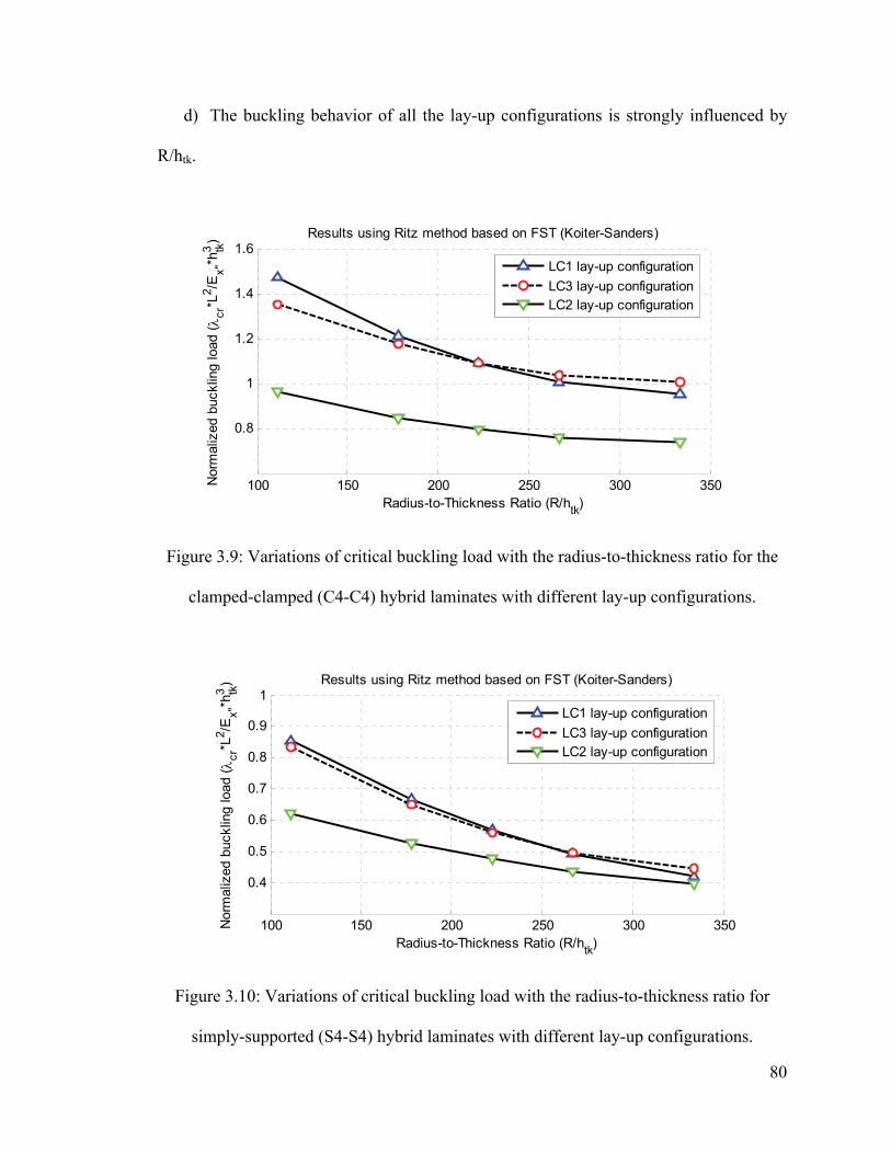
80

d) The buckling behavior of all the lay-up configurations is strongly influenced by

R/htk.


clamped-clamped (C4-C4) hybrid laminates with different lay-up configurations.

Figure 3.10: Variations of critical buckling load with the radius-to-thickness ratio for

simply-supported (S4-S4) hybrid laminates with different lay-up configurations.

100 150 200 250 300 350

0.8

1

1.2

1.4

1.6Results using Ritz method based on FST (Koiter-Sanders)

Radius-to-Thickness Ratio (R/htk)

Nor

mal

ized

buc

klin

g lo

ad ( λ

cr*L

2 /Ex"

*htk3

)


100 150 200 250 300 350

0.4

0.5

0.6

0.7

0.8

0.9

1Results using Ritz method based on FST (Koiter-Sanders)


Nor

mal

ized

buc

klin

g lo

ad ( λ

cr*L

2 /Ex"

*htk3

)


81



Table 3.6: Qualitative comparison of stiffness properties of lay-up configurations for

higher values of radius-to-thickness ratio

Fiber Orientation

Remark 900 ±450 00 Stiffness for Uniaxial End Compression Weakest Moderate Strongest

No. of plies in LC1 6 0 6 Moderate Configuration

No. of plies in LC2 0 6+6 0 Weakest Configuration

No. of plies in LC3 0 4+4 4 Strongest Configuration

Figs. 3.12 – 3.14 show the effect of the radius-to-thickness ratio on normalized critical

buckling loads. The normalized critical buckling loads corresponding to different values

of radius-to-thickness ratio of hybrid curved plates are calculated using FST based Ritz

solution and the buckling loads thus obtained are compared with that obtained using CST

100 150 200 250 300 3500.8

1

1.2

1.4

1.6Results using ANSYS


Nor

mal

ized

buc

klin

g lo

ad ( λ

cr*L

2 /Ex"

*htk3

)


82

based Ritz solution and using ANSYS®. From Figs. 3.12 – 3.14, the following


a) The normalized critical buckling loads of all lay-up configurations decrease with

the increase of radius-to-thickness ratio of the plate.

b) The lowest and highest values of buckling coefficients are obtained based on FST

and CST respectively. The buckling coefficients calculated using ANSYS® are close to

that of CST solution. In ANSYS® an 8-node shell element (SHELL99) is considered

based on the degenerated solid approach but the Ritz solution is developed based on FST

which has more degrees of freedom than the element used in ANSYS®. This is the reason

for higher values of buckling coefficient obtained using ANSYS®. In the case of

classical shell theory (CST), shear strains are omitted which is the cause for the

corresponding higher value of buckling coefficient compared to that of the other two

solutions.

c) On an average, buckling coefficient of all lay-up configurations (Figs. 3.12–3.14)

obtained based on CST is 5.8% higher than that obtained using ANSYS®. On the other

hand, buckling coefficients of LC1, LC2 and LC3 obtained based on FST are, respectively,

5.22%, 13.51% and 9.38% lower than that obtained using ANSYS®.

83


clamped-clamped (C4-C4) hybrid laminates with LC1 lay-up configuration.



100 150 200 250 300 3500.8

1

1.2

1.4

1.6

1.8


Nor

mal

ized

buc

klin

g lo

ad ( λ

cr*L

2 /Ex"

*htk3

)

CST (Ritz) [Refs. 111-112]ANSYS [Ref. 114]FST (Ritz)

100 150 200 250 300 350

0.7

0.8

0.9

1

1.1

1.2


Nor

mal

ized

buc

klin

g lo

ad ( λ

cr*L

2 /Ex"

*htk3

)

CST (Ritz)[Refs. 111-112]ANSYS [Ref. 114]FST (Ritz)

84




Normalized critical buckling loads are calculated for the rectangular hybrid laminated

curved plates (with a length/width ratio of 2.0) under uniaxial compression. The buckling

analyses are performed using Ritz method based on Koiter-Sanders shell theory. Two

boundary conditions are considered, that are, clamped at four edges (C4-C4) and simply-

supported at four edges (S4-S4). These boundary conditions are given in the Appendix B.

The effect of boundary condition on the buckling coefficient for the above mentioned

plates is shown in the Figs. 3.15 – 3.17.

As observed from Figs. 3.15 – 3.17 and as can be expected, the boundary condition has

significant influence on the buckling coefficient. In terms of critical buckling load, the

fully clamped plate has a higher buckling load than the simply-supported plate. Simply-

100 150 200 250 300 3500.9

1

1.1

1.2

1.3

1.4

1.5

1.6


Nor

mal

ized

buc

klin

g lo

ad ( λ

cr*L

2 /Ex"

*htk3

)

CST (Ritz)[Refs. 111-112]ANSYS [Ref. 114]FST (Ritz)

85

supported plates allow rotations at the boundaries which is the reason for less strength.

For lay-up configuration LC1 as can be seen in the Fig. 3.15, the buckling coefficient

difference between the values of that correspond to the clamped-clamped plate and the

simply-supported plate is in the range of about 42.66% - 53.14% and the average

difference is 45.17%. In the case of lay-up configuration LC2 as can be seen in the Fig.

3.16, the buckling coefficient difference between the values of that correspond to the

clamped-clamped plate and the simply-supported plate is in the range of about 35.02% -

46.83% and the average difference is 39.94%. On the other hand for the lay-up

configuration LC3 as can be seen in the Fig. 3.17, the buckling coefficient difference

between the values of that correspond to the clamped-clamped plate and the simply-

supported plate is in the range of about 36.22% - 54.58% and the average difference is

44.84%. Buckling coefficients of all the lay-up configurations are strongly influenced by

both R/htk ratio and boundary condition.



100 150 200 250 300 3500.4

0.6

0.8

1

1.2

1.4

1.6

1.8


Nor

mal

ized

buc

klin

g lo

ad ( λ

cr*L

2 /Ex"

*htk3

)


86





100 150 200 250 300 350

0.4

0.5

0.6

0.7

0.8

0.9

1


Nor

mal

ized

buc

klin

g lo

ad ( λ

cr*L

2 /Ex"

*htk3

)


100 150 200 250 300 3500.4

0.6

0.8

1

1.2

1.4


Nor

mal

ized

buc

klin

g lo

ad ( λ

cr*L

2 /Ex"

*htk3

)


87

3.7 CONCLUSIONS

In the present chapter, the global buckling analysis of tapered curved laminated plates has

been carried out using Ritz method based on six well-established first-order shallow shell

theories, namely, Donnell’s, Moreley’s, Love’s, Loo’s, Koiter’s and Sander’s theories.

Three types of tapered plates (two taper configurations A and B, and a hybrid

configuration), three types of lay-up configurations (LC1, LC2 and LC3), and uniaxial end

compressive load are considered. A detailed parametric study of the plates has been

conducted that includes the effects of boundary conditions, stacking sequence, taper

configurations, radius, and geometric parameters of the plates. The conclusions listed in

the following are based on the results presented in this chapter:

a) The moderately-thick and tapered curved composite plates fail by first-ply failure

before global buckling. Therefore the dimensions of tapered curved plate should be larger

than the corresponding critical size. The critical sizes depend on both radius and staking

sequence of the plates. Such critical sizes have been determined in the present work.

b) The tapered flat plate is more flexible than uniform flat plate, but the tapered

curved plate provides a better design option in terms of saving the material without any

compromise of the strength.

c) The critical buckling loads of all lay-up configurations are considerably

influenced by the stiffness ratio (Ex”/Ey”) of the ply material.

d) Classical shell theory can be used to calculate with reasonable accuracy the

critical buckling load of moderately-long plates for which Ltap/R > 0.35. The first-order

shear deformation shell theory should be used for the calculation of critical buckling load

of shorter plates for which Ltap/R < 0.35.

88

Chapter 4

Compressive Response of Tapered Curved Composite Plates Based on a

Nine-Node Composite Shell Element

4.1 INTRODUCTION

The prime objective of the present chapter is to conduct the linear global buckling

analysis of the tapered curved plates (see Fig. 1.4) using finite element method based on

first-order shear deformation shell theories. Six shell theories are used in the analysis,

that are, Donnel’s, Moreley’s, Love’s, Loo’s, Koiter’s and Sander’s theories. The

corresponding critical buckling loads are calculated and the most conservative value is

obtained. The appropriate set of shear correction factors are determined as like chapter

three and used in the buckling analyses. Buckling loads calculated using the finite

element method are compared with that of the existing experimental results and analytical

results for tapered curved composite plates based on Ritz solutions (which have been

calculated in the chapters two and three). A parametric study that encompasses the

influences of taper angle, length-to-radius ratio, stiffness ratio, stacking sequence,

boundary conditions, radius and geometric parameters of the plates on the critical

buckling load is conducted.

4.2 FORMULATION

The basic formulation based on first order shear deformation has been described in the

chapter three using the Eqs. (3.1) through (3.10). In the Eq. (3.10a), three Shear

89

Correction (SC) factors S1, S2 and S3 are given. The set of SC factors in Eq. (3.11) that

corresponds to the most conservative value of critical buckling loads is reevaluated using

the present FEM. This particular set of values is used further onwards throughout the

present work. For this purpose, a tapered plate with configuration B and having 36 layers

at the thick end with [0/90]9s lay-up and 12 layers at the thin end with [0/90]3s lay-up, that

is subjected to uni-axial end compressive loading has been analyzed using FEM method.

The plate is clamped at four edges (C4-C4) and the boundary conditions represented as

C4 are given in the Appendix C. The dimensions of the square plate are (see Fig. 1.4):

various values of the side length of the plate in the range of from 85.94 mm to 171.90

mm are considered, plate thickness at the thick end htk = 4.5 mm and the radius R = 500

mm. The material properties of the composite ply and epoxy are the same as given in

Tables 2.5 and 2.6 respectively. The critical buckling loads using these properties are

calculated and presented at the end of this section.

The total potential energy is expressed as the sum of strain energy U and the potential

energy of external load W. For a plate of dimension bLtap × subjected to uni-axial

compressionλ ,

[ ]( )dxdyEUb L

Ttap

∫ ∫=0 0

' }{}{21 εε (4.1)

where T

xzyzxyyyxxxyyyxx ][}{ 00000000 γγκκκγεεε =

(4.2) and [E’] is the stiffness matrix given in Eq. (3.10b).

dxdyx

wWb L

otap

∫ ∫ ⎟⎠⎞

⎜⎝⎛∂∂

−=0 0

2

21λ

(4.3)

90

Figure 4.1: The nine-node shell element

The nine-node Lagrange shell element with five degrees of freedom per node shown in

Fig. 4.1 is used in the present analysis. The five degrees of freedom are: the translation

displacements in x, y and z directions that are u, v and w respectively, and rotations about

y and x axes that are xϕ and yϕ respectively which are due to shear deformation. The

displacement fields and rotations are defined as:

ii iuNu ∑ ==

9

1; ii ivNv ∑=

=9

1; ii i wNw ∑ =

=9

1; ixi ix Nϕϕ ∑=

=9

1;

iyi iy Nϕϕ ∑==

9

1 (4.4)

where ),( yxNi are the Lagrange shape functions. The shape functions are given in the Appendix C.

The matrix of strains and curvatures, is expressed as:

(4.5a)

where

(4.5b)

]t (4.5c)

91

The matrix is given in the Appendix C where i = 1, 2, 3 … 9.

The first variations of strain energy U and potential energy W that are given, respectively,

by the Eqs. (4.1) and (4.3) are considered. For an element they are expressed as

(4.6)

(4.7)

where is the element nodal displacement matrix. The element stiffness matrix

and the element geometric stiffness matrix [Ge] are given by

(4.8)

(4.9)

The matrix is given in the Appendix C. The equilibrium equation of an element

is expressed as:

The Eq. (4.10) is simplified using the Eqs. (4.6) through (4.9):

0][][ =+ ∑∑ ee GK λ (4.11)

where the eigenvalues λ are the values of buckling loads. The element stiffness matrix

and the element geometric stiffness matrix [Ge] are augmented considering all of the

elements in the plate. Eq. (4.11) is solved using MATLAB® as an eigenvalue problem.

The smallest value of λ is the critical buckling load, crλ .

e

e

e

e

uW

uU

∂

∂=

∂

∂

(4.10)

92

The critical buckling loads corresponding to different values of shear correction factors

are plotted in the Figs. 4.2 and 4.3. It can be seen from these figures that the critical

buckling loads corresponding to all the six sets of shear correction factors are close to

each other for lower values of taper angle. On the other hand, at higher values of taper

angle, the values of the critical buckling loads differ relatively much. Among all the

cases, the set (S1=1, S2=5/6, S3=5/6) in the Eq. (3.11c) is the most conservative one in

terms of critical buckling load. Similar conclusion has also been made using Ritz solution

in the chapter three and this set of shear correction factors will be used further onwards in

the present work.


the clamped-clamped laminate with the configuration B based on Koiter-Sanders shell

theory.

0.5 0.55 0.6 0.65 0.7 0.75 0.8 0.85 0.9 0.95 14

5

6

7

8

9

10x 105

Taper angle (ψo)

Crit

ical

buc

klin

g lo

ad (N

/m)


93


the simply-supported laminate with the configuration B based on Koiter-Sanders shell

theory.

4.3 VALIDATION

To the authors’ knowledge, no results are available yet in the literature on the buckling

loads of the tapered curved composite plates under the action of uni-axial compression

except the other contemporary works of the present author. Therefore the comparison

with the existing works of other researchers could not be made. However, in order to

validate the formulation and analysis, first, the taper angle is set to be zero, and the

resulting uniform-thickness curved plates have been analyzed and the results have been

compared with that available in the literature for the uniform-thickness plates. For this

reason, an isotropic cylindrical panel [115] is investigated which is subjected to

uniformly distributed transverse (normal to the surface) load q, and the geometric and

materials properties are: width b = 2×R×α (α = 0.1 rad.), radius R = 2.54 m (100 in.),

length L = 0.508 m (20 in.), thickness h = 3.175x10-03 m (0.125 in.), elastic modulus E =

3.10 GPa (0.45×106 psi), Poisson ratio υ = 0.3, and transverse load q = 275.79 Pa (0.04

0.5 0.55 0.6 0.65 0.7 0.75 0.8 0.85 0.9 0.95 12

2.5

3

3.5

4

4.5

5x 105

Taper angle (ψo)

Crit

ical

buc

klin

g lo

ad (N

/m)


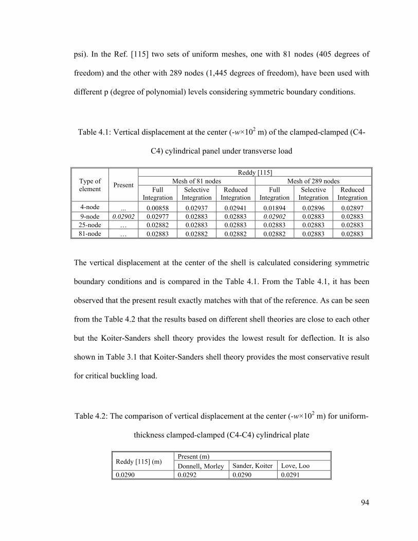
94

psi). In the Ref. [115] two sets of uniform meshes, one with 81 nodes (405 degrees of

freedom) and the other with 289 nodes (1,445 degrees of freedom), have been used with

different p (degree of polynomial) levels considering symmetric boundary conditions.

Table 4.1: Vertical displacement at the center (-w×102 m) of the clamped-clamped (C4-

C4) cylindrical panel under transverse load

Type of element Present

Reddy [115] Mesh of 81 nodes Mesh of 289 nodes

Full Integration

Selective Integration

Reduced Integration

Full Integration

Selective Integration

Reduced Integration

4-node ... 0.00858 0.02937 0.02941 0.01894 0.02896 0.02897 9-node 0.02902 0.02977 0.02883 0.02883 0.02902 0.02883 0.02883 25-node … 0.02882 0.02883 0.02883 0.02883 0.02883 0.02883 81-node … 0.02883 0.02882 0.02882 0.02882 0.02883 0.02883

The vertical displacement at the center of the shell is calculated considering symmetric

boundary conditions and is compared in the Table 4.1. From the Table 4.1, it has been

observed that the present result exactly matches with that of the reference. As can be seen

from the Table 4.2 that the results based on different shell theories are close to each other

but the Koiter-Sanders shell theory provides the lowest result for deflection. It is also

shown in Table 3.1 that Koiter-Sanders shell theory provides the most conservative result

for critical buckling load.

Table 4.2: The comparison of vertical displacement at the center (-w×102 m) for uniform-

thickness clamped-clamped (C4-C4) cylindrical plate

Reddy [115] (m) Present (m) Donnell, Morley Sander, Koiter Love, Loo

0.0290 0.0292 0.0290 0.0291

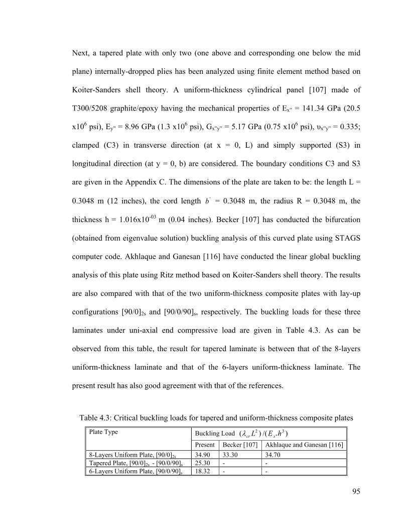
95

Next, a tapered plate with only two (one above and corresponding one below the mid

plane) internally-dropped plies has been analyzed using finite element method based on

Koiter-Sanders shell theory. A uniform-thickness cylindrical panel [107] made of

T300/5208 graphite/epoxy having the mechanical properties of Ex” = 141.34 GPa (20.5

x106 psi), Ey” = 8.96 GPa (1.3 x106 psi), Gx”y” = 5.17 GPa (0.75 x106 psi), υx”y” = 0.335;

clamped (C3) in transverse direction (at x = 0, L) and simply supported (S3) in

longitudinal direction (at y = 0, b) are considered. The boundary conditions C3 and S3

are given in the Appendix C. The dimensions of the plate are taken to be: the length L =

0.3048 m (12 inches), the cord length 'b = 0.3048 m, the radius R = 0.3048 m, the

thickness h = 1.016x10-03 m (0.04 inches). Becker [107] has conducted the bifurcation

(obtained from eigenvalue solution) buckling analysis of this curved plate using STAGS

computer code. Akhlaque and Ganesan [116] have conducted the linear global buckling

analysis of this plate using Ritz method based on Koiter-Sanders shell theory. The results

are also compared with that of the two uniform-thickness composite plates with lay-up

configurations [90/0]2s and [90/0/90]s, respectively. The buckling loads for these three

laminates under uni-axial end compressive load are given in Table 4.3. As can be

observed from this table, the result for tapered laminate is between that of the 8-layers

uniform-thickness laminate and that of the 6-layers uniform-thickness laminate. The

present result has also good agreement with that of the references.


Plate Type Buckling Load )/()( 3"

2 hEL xcrλ

Present Becker [107] Akhlaque and Ganesan [116] 8-Layers Uniform Plate, [90/0]2s 34.90 33.30 34.70 Tapered Plate, [90/0]2s - [90/0/90]s 25.30 - - 6-Layers Uniform Plate, [90/0/90]s 18.32 - -

96


In the parametric study three types of longitudinal cross-sections of the curved plates are

considered, that are, taper configurations A and B, and a hybrid configuration as shown

in the Fig. 1.4. The finite element method is used based on Koiter-Sanders shell theory.

The material properties of composite ply and epoxy used are the same as given in the

Tables 2.5 and 2.6 respectively. Based on the convergence test, the mesh size used for the

finite element analyses of taper configuration and hybrid configuration are 9×9 and

15×15 respectively. The 9×9 finite element mesh is shown in the Fig. 4.4.

Figure 4.4: The 9×9 finite element mesh for the tapered curved plate

1

3

2

5

4

7

6

9

8

11

10

13

12

15

14

17

16

19

18

20

22

21

24

23

26

25

28

27

30

29

32

31

34

33

36

35

38

37

39

41

40

43

42

45

44

47

46

49

48

51

50

53

52

55

54

57

56

58

60

59

62

61

64

63

66

65

68

67

70

69

72

71

74

73

76

75

77

79

78

81

80

83

82

85

84

87

86

89

88

91

90

93

92

95

94

96

98

97

100

99

102

101

104

103

106

105

108

107

110

109

112

111

114

113

115

117

116

119

118

121

120

123

122

125

124

127

126

129

128

131

130

133

132

134

136

135

138

137

140

139

142

141

144

143

146

145

148

147

150

149

152

151

153

155

154

157

156

159

158

161

160

163

162

165

164

167

166

169

168

171

170

172

174

173

176

175

178

177

180

179

182

181

184

183

186

185

188

187

190

189

191

193

192

195

194

197

196

199

198

201

200

203

202

205

204

207

206

209

208

210

212

211

214

213

216

215

218

217

220

219

222

221

224

223

226

225

228

227

229

231

230

233

232

235

234

237

236

239

238

241

240

243

242

245

244

247

246

248

250

249

252

251

254

253

256

255

258

257

260

259

262

261

264

263

266

265

167

169

168

171

270

273

272

275

274

277

276

279

278

281

280

283

282

285

284

286

288

287

190

189

192

291

294

293

296

295

298

297

300

299

302

301

304

303

305

307

306

309

308

311

310

313

312

315

314

317

316

319

318

321

320

323

322

324

326

325

328

327

330

329

332

331

334

333

336

335

338

337

340

339

342

341

343

345

344

347

346

349

348

351

350

353

352

355

354

357

356

359

358

361

360

1

2

3

4

5

6

7

8

9 18

17

16

15

14

13

12

11

10 19

20

21

22

23

24

25

26

27

28

29

30

31

32

33

34

35

36

37

38

39

40

41

42

43

44

45

46

47

48

49

50

51

52

53

54

55

56

57

58

59

60

61

62

63

64

65

66

67

68

69

70

71

72

73

74

75

76

77

78

79

80

81

x

y Node numberElement number

97

4.4.1 Buckling Analysis of Tapered Curved Plates

Tapered models shown in the Fig. 1.4 are considered with 36 and 12 plies at the thick end

and the thin end respectively, which results in 24 drop-off plies. The configuration at the

thick end is (0/90)9s, and that of the thin end is (0/90)3s (this lay-up configuration is

referred to as LC1 in the Table 2.7). In the analyses of taper configurations, the thickness

of the thick end htk is set to be 4.5 mm and the radius of the curved plate R is set to be

500 mm. For all the taper configurations only LC1 lay-up configuration with clamped-

clamped (C4-C4) boundary conditions is considered. In Table 4.4 the number of elements

of taper configuration B was determined based on mesh convergence test. Various

parameters, namely ply drop-off parameters, taper angle, stiffness ratio and length-to-

radius ratio are investigated to see the influences of these parameters on the buckling

loads of tapered curved plates. The results are shown in the following Figs. 4.5 through

4.10.

Table 4.4: Effect of mesh size on the critical buckling load of tapered curved plate with

taper configuration B and LC1 lay-up configuration (taper angle = 0.5 degree and radius =

500 mm)

Mesh 9 x 7 9 x 8 9 x 9 λ cr (×104 N/m) 87.2299 87.1570 87.1162


The effect of ply drop-off on critical buckling load is shown in the Figs. 4.5 and 4.6. To


corresponding to a taper angle of 0.1 degree. The thickness of the thick end is not

98

changed and the taper angle is varied with the corresponding increase in the number of

drop-off plies. The plate can be considered as a uniform-thickness plate when the

number of ply drop-off is set to zero and the taper configuration A is obtained by

dropping off twenty four plies. The plates are clamped (C4-C4) at four edges and the lay-

up configuration is LC1. In the Figs. 4.5 and 4.6, crλ denotes the critical buckling load.

Figure 4.5: The effect of ply drop-off on critical buckling load for simply-supported

plates.

0 5 10 15 20 250

0.5

1

1.5

2

2.5

3x 105


Crit

ical

buc

klin

g lo

ad ( λ

cr),

N/m

Curved Plate, R=0.5 mFlat Plate


99

Figure 4.6: The effect of ply drop-off on critical buckling load for clamped-clamped

plates.

From the Figs. 4.5 and 4.6, it is observed that the uniform-thickness curved plate is many

times stiffer than the uniform-thickness flat plate in terms of buckling behavior. It is also

observed that the tapered flat plate is less stiff than uniform flat plate. However, this

strength reduction can be compensated for if the tapered plate is made into a curved one.

It can be concluded from the Figs. 4.5 and 4.6 that the tapered curved plate provides a

better design option in terms of saving the material without any compromise of the

strength. Buckling loads of flat and curved plates vary linearly with the number of ply

drop-off. The weight savings of the tapered plate with respect to the uniform plate is

expressed as:

%100/)( ×−= PQPs WWWW (4.12)

where WP and WQ are the weights corresponding to the points marked as ‘P’ and ‘Q’

respectively in Fig. 4.6.

0 5 10 15 20 250

0.5

1

1.5

2

2.5

3

3.5x 105


Crit

ical

buc

klin

g lo

ad ( λ

cr),

N/m

Curved Plate, R=0.5 mCurved Plate, R=0.8 mCurved Plate, R=1.0 mCurved Plate, R=1.2 mCurved Plate, R=1.5 mFlat Plate

P Q

R

100

The gain of strength of the curved tapered plate with respect to the flat tapered plate can

be expressed as:

%100/)( ×−= QQRs SSSG (4.13)

where SQ and SR are the strengths corresponding to the points marked as ‘Q’ and ‘R’

respectively in Fig. 4.6.

Based on the Eq. (4.12), it is calculated that 21.96% weight can be saved by dropping-off

18 plies (corresponding to the location of ‘Q’ in the Fig. 4.6). The gain of strength of the

curved tapered plate with respect to the flat tapered plate is calculated by the Eq. (4.13).

Considering the strength property shown in Fig. 4.6, the gain of strength of the tapered

curved plate (corresponding to the location of ‘R’) with respect to the flat tapered plate

(corresponding to the point ‘Q’) is 82.47%. The details of the calculations are given in

the Appendix C. Similar conclusions have also been arrived at for other taper

configurations. Similar type of effect is presented in previous chapters in Figs. 2.4 and

3.5, where the buckling loads are calculated based on CST-based and FST-based Ritz

solution respectively. In Fig. 2.4, the buckling loads for both of the uniform and curved

plates are 0.80 % higher than that of the present FST-based FEM solution (Fig. 4.6). On

the other hand, the buckling loads shown in Fig. 3.5 are 0.46 % lower than that of the

present FST-based FEM solution (Fig. 4.6).


The effect of taper angle of the curved plates on the critical buckling load is compared

with that of obtained CST based Ritz solution and FST based Ritz solution. The

comparison is shown in the Fig. 4.7 where the size of the plate is decreased with the

101

increase of taper angle while keeping the thickness of the thick section unchanged. The

maximum and minimum edge lengths of the tapered curved square plate are 859.4 mm

corresponding to a taper angle of 0.1 degree and 85.94 mm corresponding to a taper angle

of 1.0 degree respectively. In the Fig. 4.7, crλ denotes the critical buckling load.

As can be observed from Fig. 4.7, the critical buckling load using three different methods

increases as the taper angle is increased, because the plate becomes shorter (without

changing the thickness) with the increase of taper angle. The buckling loads in the Refs.

[112] and [116] are, respectively, calculated using Ritz method based on CST and FST.

The buckling results FST based FEM solution are close to FST based Ritz solution as the

both of these methods are based on first-order shear deformation theory. At lower values

of taper angle, buckling loads obtained using different methods do not vary significantly.

On the other hand, at the higher values of taper angle the critical buckling loads obtained

using three different methods differ relatively much. It can also be observed that in all the

three cases, the critical buckling load varies nonlinearly with the variation of taper angle.

Figure 4.7: Effect of taper angle on the critical buckling load for clamped-clamped

tapered curved plate with the taper configuration B and the LC1 lay-up configuration.

0.1 0.2 0.3 0.4 0.5 0.6 0.7 0.8 0.9 10

2

4

6

8

10

12x 105

Taper angle (ψo)

Crit

ical

buc

klin

g lo

ad ( λ

cr),

N/m CST (Ritz) [Ref.112]

FST (FEM)

FST (Ritz) [Ref. 116]

102


The normalized buckling loads of the plates of different sizes are calculated and

compared with that of CST (Ritz) [112] and FST (Ritz) [116]. The lay-up configuration is

LC1 and the clamped-clamped (C4-C4) boundary conditions are considered. The material

properties of composite ply and epoxy are used same as given in the Tables 2.5 and 2.6

respectively. The results are presented in the Fig. 4.8, wherein R denotes the radius of the

plate, htk denotes the thickness at the thick end, crλ denotes the critical buckling load, Ltap

denotes the length of taper section and Ey” denotes the elastic modulus of composite

material in the fiber direction.

The normalized buckling load called herein as the buckling coefficient decreases with the

decrease of length-to-radius ratio of the tapered curved plate. Buckling coefficient using

FST based FEM solution is close to that of the FST based Ritz solution. But buckling

coefficients using FEM solution and FST based Ritz solution depart away from that of

CST based Ritz solution with the increase of thickness of the plate as the rotations ( xϕ

and yϕ ) play an important role with the increase of plate thickness. The buckling load

using FEM is compared with the one using CST and the error is close to 10%

corresponding to the moderately-long plate (Ltap/R = 0.25). The error percentage

increases with the decrease of length-to-radius ratio (Ltap/R) as the plate becomes shorter.

103


clamped tapered curved laminate with the lay-up configuration LC1 and the taper

configuration B.

4.4.1.4 The effect of the stiffness ratio

The variation of critical buckling load is shown in the Figs. 4.9 and 4.10 as a function of

stiffness ratio Ex”/Ey” for each lay-up configuration. The results were obtained by

changing the value of Ex”. In the Figs. 4.9 and 4.10, Ex” and Ey” denote, respectively, the

elastic moduli of composite ply material in the fiber direction and in the direction

transverse to the fiber direction. As was expected, the critical buckling load in all the

three cases increases linearly with increasing stiffness ratio values. For the lower values

of stiffness ratio, the values of the critical buckling loads of all the three lay-up

configurations are very close to each other. But for higher values of stiffness ratio the

critical buckling loads of the three lay-up configurations differ much between themselves.

This effect is more pronounced in the case of LC1.

0.1 0.2 0.3 0.4 0.5 0.6 0.7 0.8 0.90.5

1

1.5

2

2.5

3

Length-to-Radius Ratio(Ltap/R)

Crit

ical

buc

klin

g lo

ad ( λ

cr*L

tap

2/E

x"*h

tk3)

CST (Ritz) [112]FST (FEM)FST (Ritz) [116]

104

Figure 4.9: Effect of stiffness ratio on critical buckling load for clamped-clamped tapered

curved laminate with the taper configuration B.

Figure 4.10: Effect of stiffness ratio on critical buckling load for simply-supported

tapered curved laminate with the taper configuration B.

4.4.2 Buckling Analysis of Hybrid Curved plates

Laminates with only taper configuration have been studied in the previous sections of this

chapter. The hybrid configuration (consisting of both tapered and uniform-thickness

sections) is taken into account in the present sub-section. The tapered section of hybrid

10 15 20 252

4

6

8

10

12x 105

Ex"/Ey"

Crit

ical

buc

klin

g lo

ad ( λ

cr),



10 15 20 252

3

4

5

6

7x 105

Ex"/Ey"

Crit

ical

buc

klin

g lo

ad ( λ

cr),



105

plate is considered to have the taper configuration B. For the analyses of hybrid

configuration three types of lay-up configurations, namely LC1, LC2 and LC3 given in the

Table 2.7 are considered. For the buckling analyses, the total plate length L = 229.2 mm,

width b = 114.6 mm and the material properties given in Tables 2.5 and 2.6 are

considered. According to the first-ply failure analysis, the hybrid plates with the above

mentioned lay-up configurations will not fail by first-ply failure before global buckling.

Two parameters radius-to-thickness ratio and boundary condition are investigated as to

their effects on the critical buckling load of hybrid curved plate. With the increase of

radius-to-thickness ratio, the plate becomes more flat as the radius is increased without

changing the thickness at the thick end. The results are shown in the following Figs. 4.11

through 4.18.

4.4.2.1 Influence of Lay-Up Configurations

The normalized critical buckling loads of three lay-up configurations LC1, LC2 and LC3

are calculated using finite element method and are compared in the Figs. 4.11 - 4.12. The

buckling loads are calculated for clamped-clamped (C4-C4) boundary conditions. The

effect of radius-to-thickness ratio on buckling load is also evaluated in the Figs. 4.11 -

4.12. In these figures, R denotes the radius, htk denotes the thickness at the thick end, crλ

denotes the critical buckling load, L denotes the total length of hybrid plates and Ex”

denotes the elastic modulus of composite material in the fiber direction.

106

Figure 4.11: Variation of buckling coefficients with the radius-to-thickness ratio for the


Figure 4.12: Variation of critical buckling load with the radius-to-thickness ratio for

simply- supported (S4-S4) hybrid laminates with different lay-up configurations.

From Figs. 4.11 - 4.12, the following observations are made:

a) The lay-up configuration LC2 is the weakest one among all lay-up configurations.

100 150 200 250 300 350

0.8

1

1.2

1.4

1.6


Nor

mal

ized

buc

klin

g lo

ad ( λ

cr*L

2 /Ex"

*htk3

)


100 150 200 250 300 3500.4

0.5

0.6

0.7

0.8

0.9

1


Nor

mal

ized

buc

klin

g lo

ad ( λ

cr*L

2 /Ex"

*htk3

)


107

b) The rate of change of buckling load of lay-up configuration LC3 is lesser than that

of lay-up configuration LC1. The buckling coefficient of LC1 is higher than that of

LC3 for smaller values of radius-to-thickness ratio (R/htk < 245 for clamped-

clamped plate and R/htk < 260 for simply-supported plate). In the case of larger

values of radius-to-thickness ratio (R/htk > 245 for clamped-clamped plate and

R/htk > 260 for simply-supported plate), LC3 is stronger than LC1.

c) In all the cases, the value of the buckling coefficient decreases nonlinearly with

the increase of radius-to-thickness ratio. The values of buckling coefficient

become close to each other at larger values of R/htk ratio as the plate becomes

flatter. In the case of plate with larger radius, the effect of radius has less

influence on the buckling coefficient and the buckling behavior of the plate

largely depends on the orientation of fiber angle. For uniaxial compressive load,

the fibers parallel to the direction of the applied load are the strongest ones and

the fibers perpendicular to the direction of the applied load are the weakest ones.

A quantitative comparison of relative stiffness of three lay-up configurations is

given in the Table 3.6. Lay-up configuration LC3 is the strongest as it is made of

two types of plies: moderately stiff plies and stiffest plies. Lay-up configuration

LC2 is the weakest one as it is constructed of the moderately stiff plies only. On

the other hand, lay-up configuration LC1 is the moderately stiff as two extreme

types of plies namely, the weakest plies and strongest plies, are used to construct

it.

d) The buckling behavior of all the lay-up configurations is strongly influenced by

R/htk.

108

Figs. 4.13 – 4.15 show the effect of the radius-to-thickness ratio on normalized critical

buckling load. The normalized critical buckling loads corresponding to different values of

radius-to-thickness ratio of hybrid curved plates are calculated using finite element

method based on Koiter-Sanders shell theory. The buckling coefficients are compared

with that obtained using Ritz method based on CST and using element SHELL99 of

ANSYS®. From Figs. 4.13 – 4.15, the following observations are made.

a) The normalized critical buckling loads of all lay-up configurations decrease with

the increase of radius-to-thickness ratio.

b) The lowest and highest values of buckling coefficients are obtained using the

present FEM solution and CST based on Ritz solution respectively. In the case of

classical shell theory (CST), shear strains are omitted which is the cause for the

corresponding higher values of buckling loads compared to that of the other two

(present FEM and ANSYS) solutions. The buckling coefficient calculated using

FEM is lower than that of the ANSYS®. Because FEM solution is based on a

nine-node shell element which has more degrees of freedom than that of the

SHELL99 of ANSYS®.

c) On an average, the buckling coefficients of LC1 lay-up configuration (Fig. 4.13)

obtained based on ANSYS® and the present FEM solution are, respectively, 5.5%

and 6.47% lower than that obtained using CST based Ritz solution.

d) On an average, the buckling coefficients of LC2 lay-up configuration (Fig. 4.14)

obtained based on ANSYS® and the present FEM solution are, respectively, 4.2%

and 10.67% lower than that obtained using CST based solution.

109

e) On an average, the buckling coefficients of LC3 lay-up configuration (Fig. 4.15)

obtained based on ANSYS® and the present FEM solution are, respectively,

4.07% and 7.70% lower than that obtained using CST based solution.





100 150 200 250 300 3501

1.2

1.4

1.6

1.8


Nor

mal

ized

buc

klin

g lo

ad ( λ

cr*L

2 /Ex"

*htk3

)

CST (Ritz) [112]ANSYS [114]FST (FEM)

100 150 200 250 300 350

0.7

0.8

0.9

1

1.1

1.2


Nor

mal

ized

buc

klin

g lo

ad ( λ

cr*L

2 /Ex"

*htk3

)

CST (Ritz) [112]ANSYS [114]FST (FEM)

110




Normalized critical buckling loads are calculated for the rectangular hybrid laminated

curved plates (with a length/width ratio of 2.0) under uniaxial end compression. The

buckling analyses are performed using finite element method based on Koiter-Sanders

shell theory. Two types of boundary conditions are considered, that are, clamped at four

edges (C4-C4) and simply supported at four edges (S4-S4). These boundary conditions

are given in the Appendix C. The effect of radius-to-thickness ratio on the buckling

coefficient for the above mentioned plates is shown in the Figs. 4.16- 4.18.

100 150 200 250 300 3501

1.1

1.2

1.3

1.4

1.5

1.6

1.7


Nor

mal

ized

buc

klin

g lo

ad ( λ

cr*L

2 /Ex"

*htk3

)CST (Ritz) [112]ANSYS [114]FST (FEM)

111

As observed from Figs. 4.16- 4.18 and as can be expected, the boundary condition has

significant influence on the buckling coefficient. In terms of critical buckling load, the

fully clamped plate has a higher buckling load than the simply-supported plate. Simply

supported plates allow rotations at the boundaries which is the reason for less strength.

For lay-up configuration LC1 as can be seen in the Fig. 4.16, the difference between the

buckling coefficient values that correspond to the clamped-clamped plate and the simply-

supported plate is in the range of about 39.88% - 50.95% and the average difference is

43.50%. In the case of lay-up configuration LC2 as can be seen in the Fig. 4.17, the

difference between the buckling coefficient values that correspond to the clamped-

clamped plate and the simply-supported plate is in the range of about 31.78% - 42.58%

and the average difference is 37.10%. On the other hand for the lay-up configuration LC3

as can be seen in the Fig. 4.18, the difference between the buckling coefficient values that

correspond to the clamped-clamped plate and the simply-supported plate is in the range

of about 36.30% - 51.56% and the average difference is 42.92%. Buckling coefficients of

all the lay-up configurations are strongly influenced by both R/htk ratio and the boundary

condition.

112


configuration for different boundary conditions using FEM.



100 150 200 250 300 3500.4

0.6

0.8

1

1.2

1.4

1.6

1.8


Nor

mal

ized

buc

klin

g lo

ad ( λ

cr*L

2 /Ex"

*htk3

)


100 150 200 250 300 3500.4

0.5

0.6

0.7

0.8

0.9

1

1.1


Nor

mal

ized

buc

klin

g lo

ad ( λ

cr*L

2 /Ex"

*htk3

)


113



4.5 CONCLUSIONS

In the present chapter, the buckling analysis of tapered curved laminated plates has been

carried out using finite element method based on six well-established first-order shallow

shell theories, namely, Donnell’s, Moreley’s, Love’s, Loo’s, Koiter’s and Sander’s

theories. Three types of tapered plates (taper configurations A and B, and a hybrid

configuration), three types of lay-up configurations (LC1, LC2 and LC3), and uniaxial end

compressive load are considered. A detailed parametric study of the plates has been

conducted that includes the influences of boundary condition, stacking sequence, taper

configuration, radius, and geometric parameters of the tapered curved plates. The

conclusions listed in the following are based on the results presented in this chapter:

a) Any of the previously mentioned shell theories can be used for the buckling

analysis of uniform or tapered curved plates. But the Sander’s and the Koiter’s

shell theories provide the most conservative result.

100 150 200 250 300 3500.4

0.6

0.8

1

1.2

1.4


Nor

mal

ized

buc

klin

g lo

ad ( λ

cr*L

2 /Ex"

*htk3

)


114

b) The uniaxial compressive strength can be increased significantly by making the

tapered plate into a curved one and a considerable amount of material can also be

saved.

c) The critical buckling loads of all lay-up configurations are considerably influenced

by the stiffness ratio (Ex”/Ey”) of the ply material. In the present analysis, the value

of Ex” was varied without changing the value of Ey”. As a result, plate becomes

stiffer in the longitudinal direction with the increase of the stiffness ratio (Ex”/Ey”)

and this influenced significantly to increase the critical buckling load.

d) In the case of present FEM solution, classical shell theory can be used to calculate

with reasonable accuracy the critical buckling loads of moderately-long plates for

which Ltap/R > 0.25. The first-order shear deformation shell theory should be used

for the calculation of critical buckling loads of shorter plates for which Ltap/R <

0.25. In the case of FST based Ritz solutions of chapter three, this ratio Ltap/R is to

be 0.35. Because, the present FEM solution is closer to CST based Ritz solution

compared to that of the FST based Ritz solution. For this reason, shorter plate can

be used if the FEM based solution is being used in the calculation of critical

buckling load.

e) At higher values of radius, lay-up configurations LC3, LC1 and LC2 become the

strongest, moderate and weakest laminates respectively.

115

Chapter 5

Non-Linear Buckling Analysis of Tapered Curved Composite Plates

Based on a Simplified Methodology

5.1 INTRODUCTION

The first objective of this chapter is to conduct the fully non-linear analysis of the tapered

curved plate without considering the effect of ply failure on the response of the tapered

curved plate using the finite element method based on first-order shear deformation shell

theories. Two non-linear shell theories are used in the analysis, that are, Donnel’s and

Sanders’s theories. The corresponding stability limit loads are calculated and the most

conservative value is obtained. The second objective is to calculate the linearized

buckling loads considering the singularity of the tangent stiffness matrix. The third

objective is to determine the stability limit load using a simplified methodology that

involves only two load steps. A parametric study that encompasses the effects of taper

angle, length-to-height ratio, radius, radius-to-thickness ratio, and geometric parameters

of the plates is also conducted.

In the present work, the buckling response of curved composite plates with longitudinal

internal ply-drop-off configurations as shown in Fig. 5.1 is investigated. Longitudinal-

ply-drop-off tapers are those in which the internal discontinuities of the laminate are

parallel to the direction of the applied load. In the Fig. 5.1, htk and htn denote the

thicknesses at the thick end and thin end respectively; Ltk, Ltap and Ltn denote the lengths

116

of thick, taper and thin section respectively; R, b and b’ denote the radius, the width and

the cord length of curved plates respectively; and (uo, vo, wo) denotes the mid-plane

displacement field with reference to the global coordinate system (x, y, z). The taper

configuration has five resin pockets: four small resin pockets are distributed

symmetrically with respect to the mid-plane and the fifth one is designed combining the

two small resin pockets. Every small resin pocket is formed by dropping-off three

composite plies and there are continuous composite plies above and below each resin

pocket. The hybrid configuration is obtained by combining the tapered and uniform-

thickness sections as shown in the Fig. 5.1 wherein L denotes the total length.

Figure 5.1: Different longitudinal cross-sections of curved plate.

117

5.2 FORMULATION

The basic formulation based on first order shear deformation has been described in the

chapter three using the Eqs. (3.1) through (3.10). In the Eq. (3.10a), three Shear

Correction (SC) factors S1, S2 and S3 are given. It has been shown in the previous

chapters three and four that the set (S1=1, S2= S3=5/6) in the Eq. (3.11c) is the most

conservative one in terms of critical buckling load. This set of shear correction factors

will be used in the present non-linear analyses.

The total potential energy is expressed as the sum of strain energy U and the potential

energy of external load W. For the tapered plate of dimension bLtap × subjected to uni-

axial compression Px,

[ ]{ }

[ ]{ } [ ]{ }

[ ]{ } [ ]{ }

NNNLLNLL

b L

NT

N

b L

LT

N

b L

NT

L

b L

LT

L

b LT

UUUU

dxdyEdxdyE

dxdyEdxdyE

dxdyEU

taptap

taptap

tap

+++=

++

+=

=

∫ ∫∫ ∫

∫ ∫∫ ∫

∫ ∫

0 0

'

0 0

'

0 0

'

0 0

'

0 0

'

][][21][][

21

][][21][][

21

][][21

εεεε

εεεε

εε

(5.2)

where and [E’] are given in the Eq. (3.10b).

The nine-node Lagrange element with five degrees of freedom per node shown in Fig. 4.1

is used in the analysis. The five degrees of freedom are: the translation displacements in

x, y and z directions that are u, v and w respectively, and rotations about y and x axes that

dyuPWtapLxo

b

x =∫−= |0

(5.1)

118

are xϕ and yϕ which are due to shear deformation. The displacement fields and rotations

are defined as:

ii iuNu ∑==

9

1 ; ii ivNv ∑==

9

1 ; ii iwNw ∑==

9

1 ; ixi ix Nϕϕ ∑==

9

1 ; iyi iy Nϕϕ ∑==

9

1 (5.3)

where ),( yxNi are the Lagrange shape functions. The shape functions are given in the

Appendix C.

The linear part of the matrix of strains and curvatures, is expressed as:

(5.4)

]T

where the matrix is given in the Appendix D with i = 1, 2, 3 … 9 and the non-liner

part of the matrix of strains and curvatures, is expressed as:

(5.5)

The matrices [H] and [S] are given in the Appendix D. The first variation of potential

energy W given by Eq. (5.1), and the first and second variations of strain energy U given

by Eq. (5.2) are considered. They are expressed as:

(5.6)

(5.7)

(5.8)

where is the element nodal displacement matrix.

Further, element nodal load matrix ][ eF , element stiffness matrix and element

tangent stiffness matrix are written as:

119

( )tapLx

Txxxe NPNPNPF == |]0,0,0,0,,........0,0,0,0,,0,0,0,0,[][ 921 (5.9)

[ ] [ ][ ] [ ] [ ][ ][ ]

[ ] [ ] [ ][ ] [ ] [ ] [ ][ ][ ]⎥⎥⎦

⎤⎟⎟⎠

⎞⎜⎜⎝

⎛Ω+⎟⎟

⎠

⎞⎜⎜⎝

⎛Ω+

⎟⎟⎠

⎞⎜⎜⎝

⎛Ω+

⎢⎢⎣

⎡⎟⎟⎠

⎞⎜⎜⎝

⎛Ω=

∫∫

∫∫

ΩΩ

ΩΩ

dSHEHSdBEHS

dSHEBdBEBK

TTL

TT

TLL

TLe

''

''

21

21][

(5.10)

[ ] [ ][ ] [ ] [ ][ ][ ]

[ ] [ ] [ ][ ] [ ] [ ] [ ][ ][ ]

[ ] [ ][ ] [ ] [ ][ ]⎥⎥⎦

⎤⎟⎟⎠

⎞⎜⎜⎝

⎛Ω+⎟⎟

⎠

⎞⎜⎜⎝

⎛Ω+

⎟⎟⎠

⎞⎜⎜⎝

⎛Ω+⎟⎟

⎠

⎞⎜⎜⎝

⎛Ω+

⎟⎟⎠

⎞⎜⎜⎝

⎛Ω+

⎢⎢⎣

⎡⎟⎟⎠

⎞⎜⎜⎝

⎛Ω=

∫∫

∫∫

∫∫

ΩΩ

ΩΩ

ΩΩ

dSNSdSNS

dSHEHSdBEHS

dSHEBdBEBK

NT

LT

TTL

TT

TLL

TLeT

''

''][

(5.11)

The matrices [H], [S], [NL] and [NN], and the matrix of shape functions [Ni] are given in

the Appendix D.

The equilibrium equations for an element are expressed as:

The non-linear Eq. (5.12) is simplified using the Eqs. (5.6), (5.7), (5.9) and (5.10) in

terms of element stiffness matrix , element nodal load matrix }{ eF and the element

nodal displacement matrix }{ eu as:

{ }( )[ ] { } { }∑∑ = eee FuuK (5.13)

The Newton-Raphson solution procedure for the r-th iteration can be expressed as:

{ }( ) { } { } { }( ) { } 111 ][][ −−− −=∂ rrrrT uuKFuuK (5.14)

where [KT] denotes the tangent stiffness matrix of the structure, {F} denotes the load

matrix of the structure, [K] denotes the stiffness matrix of the structure, and {u} denotes

the displacement matrix of the structure. The solution at the r-th iteration is then given by

ee uW

uU

∂∂

=∂∂ (5.12)

120

{ } { } { }rrr uuu ∂+= −1 (5.15)

The linearized buckling loads are determined considering the singularity of the tangent

stiffness matrix. The details of linearized buckling analysis has been explained in the Ref.

[91] which is summarized in the following.

The stiffness matrices that correspond to two successive load steps represented by (t-∆t)

and t are [t-∆tK] and [tK] respectively, and the corresponding vectors of externally applied

loads are {t-∆tPx} and {tPx}. In the linearized buckling analysis it is assumed that the

stiffness varies linearly with the linear variation of the applied load and at any load step τ,

γτ

=−−

Δ−

Δ−

][][][][

KKKK

ttt

tt

(5.16)

and

γτ

=−−

Δ−

Δ−

}{}{}{}{

xtt

xt

xtt

x

PPPP

(5.17)

where γ is a scaling factor. At the state of buckling, the tangent stiffness matrix is

singular and the condition for calculating γ is:

0]det[ =Kτ (5.18)

or, equivalently,

0}]{[ =uKτ (5.19)

Substituting from the Eq. (5.16) into the Eq. (5.19) , the eigenproblem is obtained as:

}]{[}]{[ uKuK ttt Δ−Λ= (5.20) and

γγ 1−

=Λ (5.21)

121

The eigenvalues iΛ in the Eq. (5.21) are all positive and the smallest values ......, 21 ΛΛ

are of interest. The linearized buckling load is given by:

}){}({}{}{ 1 xtt

xt

xtt

Bucklingx PPPP Δ−Δ− −Λ+= (5.22)

In the present work, the arc-length method of Ref. [77] is considered for the fully non-

linear buckling analysis. In the case of arc-length method, both the displacement and load

are iterative according to Crisfield’s arc-length method [77] and the incremental

displacement { }ru∂ is expressed in terms of displacement and load. Moreover, in the

present work, post-buckling analysis is carried out without considering the effect of ply

failure and the stability limit load (non-linear buckling load) is evaluated from the load-

deflection curve. Numerical integration is considered to evaluate the stiffness matrix and

the tangent stiffness matrix using the appropriate Gauss quadrature.

5.3 VALIDATION

To the author’s knowledge, no results are available yet in the literature on the non-linear

buckling analysis of the tapered curved composite plates under the action of uni-axial

compression. Therefore the comparison with the existing works could not be made. In

order to validate the formulation and analysis, first, the taper angle is set to be zero, and

the resulting uniform-thickness plates have been analyzed and the results have been

compared with that available in the literature for the uniform-thickness plates. For this

purpose, the deflection of a shallow curved plate hinged on straight edges and free on the

curved edges [62] is calculated using the Sanders’s shell theory. The geometric and

material parameters used are: width b = 2×R×α (α = 0.1 rad.), radius R = 0.0254 m (1in.),

length L = 0.508 m (20 in.), thickness h = 3.175x10-03 m (0.125 in.), elastic modulus E =

122

3.10 GPa (0.45×106 psi) and Poisson ratio υ = 0.3. Point load at the center of the plate is

used with a load step of P = - 444.82 N and a total of 12 load steps are considered. For

this non-linear analysis, full integration of stiffness coefficients and symmetric boundary

conditions are considered. The deflection versus load curve is compared in the Fig. 5.2

for different mesh sizes (in the Fig. 5.2, for example, N9-6x6 represents the 6x6 mesh

using nine-node element). As can be observed the results obtained using nine-node

element are in close agreement with those given by Reddy [62].

Figure 5.2: Deflection versus load curve for the hinged-free curved plate based on

Sanders’s shell theory.

A uniform-thickness cylindrical panel with ply configuration [02/902]s and made of

T300/5208 graphite/epoxy material having the mechanical properties of Ex” = 181 GPa,

Ey” = Ez” = 10.3 GPa, Gx”y” = Gx”z” = Gy”z” = 7.10 GPa, υx”y” = υx”z” = υy”z” = 0.28 and the

geometrical properties of length L = 150 mm, width b = 157.05 mm, radius R = 150 mm,

thickness h = 1 mm and cross sectional area at the curved end A = 157.05 mm2 has been

0 0.005 0.01 0.015 0.02 0.025 0.030

1000

2000

3000

4000

5000

6000

Deflection at the Center (m)

Poi

nt L

oad

(N)

N9-6x6N9-8x8N9-12x12N25-1x1 [62]

F

H

H

F

P

123

investigated by Kweon and Hong [118]. In this reference, continuum non-linear analysis

has been carried out using 8-node degenerative shell element and updated Lagrangian

formulation without considering the effect of ply failure. However, in the present study,

fully non-linear analysis is carried out using nine-node Lagrange shell element and

Sanders shell theory without considering the failure effect. The arc-length method is used

to solve the non-linear equations. The load-deflection curve is plotted in the Fig. 5.3 from

which the stability limit load is calculated as 129 MPa (the details of limit load

calculation are given in the Appendix E) but in the Ref. [118] its value is given as 123.10

MPa. Deflections calculated based on two shell theories are close to each other but

Sanders’s theory provides a more conservative result. This shell theory will be used

further onwards in the present work.

Figure 5.3: Load-deflection curve for uniform-thickness curved plate with ply

configuration [02/902]s.

0 1 2 3

x 10-4

0

0.5

1

1.5

2

2.5

3

3.5x 108

Maximum Transverse Deflection (m)

Load

per

Uni

t Are

a (P

x/A),

Pa

SanderDonnel

Stability Limit

124

Alternatively, the stability limit load of cylindrical panel with ply configuration [02/902]s

is predicted from the linearized critical loads. The calculation of linealized critical load is

performed based on a pre-stressed structure under a certain load vector {Fbase} and can be

expressed as:

{Fbase} = λbase{Fref} (5.23)

where {Fref} denotes the reference pre-stress load vector and λbase denotes the scalar base

load.

To perform this type of linearized analysis, the selected load {Fbase} is first applied in a

single load step and the modified Newton-Raphson equilibrium iteration is performed.

The tangent stiffness matrix of the structure [KT] corresponding to the equilibrium state is

obtained. At the succeeding step a trial load increment is applied and the stiffness matrix

[K] due to stress and displacement increment of this trial load step is calculated. A basic

assumption of the linearized analysis is that the structure behaves linearly before the

critical load is reached. Based on this assumption, the pre-stressed load {Fbase} is applied

to find out the corresponding critical load, so that the tangent stiffness matrix [KT] is

completely degraded. To find out this additional load level, a generalized eigen-analysis

procedure is applied. If the eigenvalue extraction based on this fundamental load level

gives a critical scalar load ∆λcr, then the predicted and linearized critical scalar load λcr,

shown in the Fig. 5.4, is given by

λcr = ∆λcr + λbase (5.24)

At various base load levels, different linearized critical loads may be predicted, and if the

stability limit does exist for the structure, the curve formed by connecting these predicted

critical loads should intersect the non-linear load-deflection curve at the point of

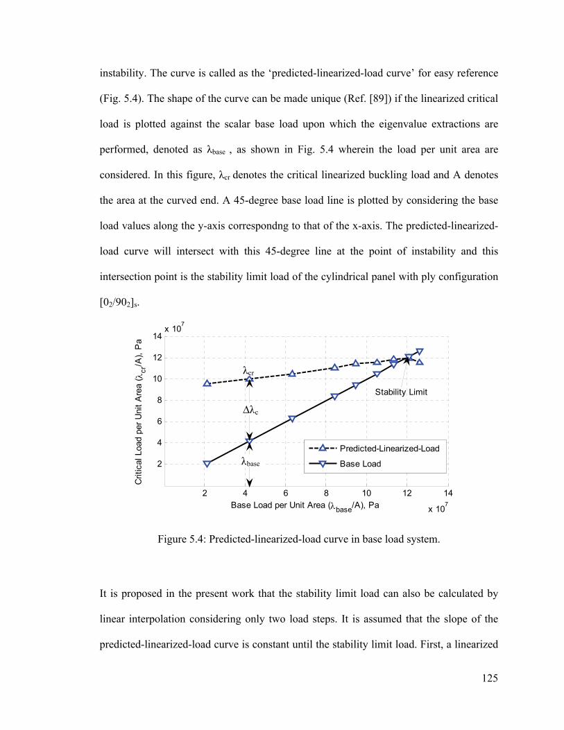
125

instability. The curve is called as the ‘predicted-linearized-load curve’ for easy reference

(Fig. 5.4). The shape of the curve can be made unique (Ref. [89]) if the linearized critical

load is plotted against the scalar base load upon which the eigenvalue extractions are

performed, denoted as λbase , as shown in Fig. 5.4 wherein the load per unit area are

considered. In this figure, λcr denotes the critical linearized buckling load and A denotes

the area at the curved end. A 45-degree base load line is plotted by considering the base

load values along the y-axis correspondng to that of the x-axis. The predicted-linearized-

load curve will intersect with this 45-degree line at the point of instability and this

intersection point is the stability limit load of the cylindrical panel with ply configuration

[02/902]s.

Figure 5.4: Predicted-linearized-load curve in base load system.

It is proposed in the present work that the stability limit load can also be calculated by

linear interpolation considering only two load steps. It is assumed that the slope of the

predicted-linearized-load curve is constant until the stability limit load. First, a linearized

2 4 6 8 10 12 14

x 107

2

4

6

8

10

12

14x 107

Base Load per Unit Area (λbase/A), Pa

Crit

ical

Loa

d pe

r Uni

t Are

a ( λ

cr/A

), P

a

Predicted-Linearized-Load

Base Load

Stability Limit

λcr

λbase

∆λc

126

buckling analysis based on the pre-stress load (b1) is performed, and an approximated

critical load (p1) is obtained (see Fig. 5.5). Then a suitable second base load (b2) is

applied to the structure and iterations are carried out until equilibrium. This configuration

of the structure is taken as the base state upon which another linearized buckling analysis

is performed to obtain a new predicted critical load (p2). Finally, on a λcr-λbase graph,

extrapolation from points (b1, p1) and (b2, p2) is made to find out the intersection point.

The linear interpolation is expressed for the prediction of the stability limit load as:

Stability ;1 2

121

mbmpLoadLimit

−−

= (5.25)

12

122 bb

ppm−−

= (5.26)

where m2 is the slope of the predicted-linearized-load curve, b1 and b2 are the base loads,

and p1 and p2 are the linearized critical loads corresponding to the base loads b1 and b2

respectively.

Figure 5.5: Prediction of stability limit load using the simplified methodology for

uniform-thickness curved plate with ply configuration [02/902]s.

2 4 6 8 10 12 14

x 107

2

4

6

8

10

12

14x 107

Base Load per Unit Area (λbase/A), Pa

Crit

ical

Loa

d pe

r Uni

t Are

a ( λ

cr/A

), P

a

Predicted-Linearized-LoadBase Load

Stability Limitp1

p2

b1

b2

127

In the Table 5.1, the stability limit load per unit area predicted based on the present

simplified methodology is compared with that obtained using fully non-linear analysis. It

is observed from the Table 5.1, the stability limit load per unit area predicted based on the

simplified methodology is 6.76 % lower than that obtained from fully non-linear analysis

(for corresponding load-deflection curve, see Fig. 5.3).

Table 5.1: Comparison of stability limit load per unit area for the cylindrical panel with

ply configuration [02/902]s

Plate Type

Stability Limit Load per Unit Area Based on Simplified Methodology (MPa)

Stability Limit Load per Unit Area Based on Fully Non-Linear Analysis (MPa)

Uniform Curved 120.27 129


In the parametric study two types of longitudinal cross-sections of the curved plates are

considered, that are, taper configuration and hybrid configuration as shown in the Fig.

5.1. The non-linear buckling analysis is carried out using nine-node Lagrange shell

element based on Sander’s theory. The material properties of composite material and

epoxy used are the same as given in the Tables 2.5 and 2.6 respectively. Based on the

convergence test, the number of elements used in the finite element analysis of taper

configuration and hybrid configuration are 9×9 and 15×15 respectively. The 9×9 finite

element mesh is shown in the Fig. 4.4.

128

5.4.1 Non-Linear Buckling Analyses of Tapered Curved Plates

For the analysis of tapered curved plates, three types of non-linear buckling analyses are

considered, that are, fully non-linear buckling, linearized buckling and simplified non-

linear buckling analysis. The fully non-linear buckling analysis employs a non-linear

static analysis with gradually increasing load to seek the load level at which the structure

becomes unstable and this load level is known as the stability limit load. The basic

assumption of the linearized buckling analysis is that the structure behaves linearly before

the critical load is reached. In case of simplified non-linear buckling analysis, the stability

limit is calculated by linear interpolation considering only two load steps and it is

assumed that the slope of the predicted-linearized-load curve is constant until the stability

limit point.

Taper configuration shown in the Fig. 5.1 is considered with 36 and 12 plies at thick and


end is [0/90]9s, and that of the thin end is [0/90]3s. In the fully non-linear analysis of taper

configuration, the height of the thick end htk is to be taken as 4.5 mm and the radius of

curved plate R is set to be 500 mm. Various values for parameters, namely the critical

length-to-height ratio, radius, and taper angle are investigated to see the influences of

these parameters on the buckling loads of tapered curved plates. The results are shown in

the following Figs. 5.6 through 5.8.

The fully non-linear analysis of clamped-clamped tapered curved square plate with the

side length of 0.8594 m is carried out using the Crisfield’s arc-length method [77]. The

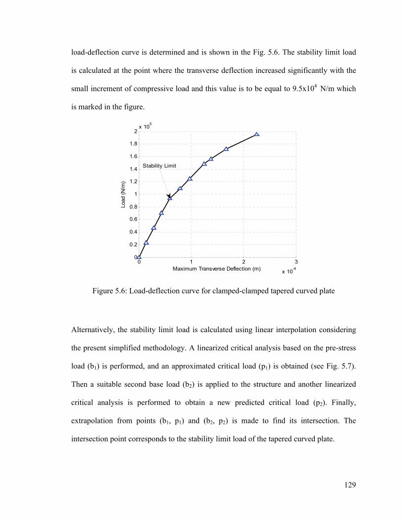
129

load-deflection curve is determined and is shown in the Fig. 5.6. The stability limit load

is calculated at the point where the transverse deflection increased significantly with the

small increment of compressive load and this value is to be equal to 9.5x104 N/m which

is marked in the figure.

Figure 5.6: Load-deflection curve for clamped-clamped tapered curved plate

Alternatively, the stability limit load is calculated using linear interpolation considering

the present simplified methodology. A linearized critical analysis based on the pre-stress

load (b1) is performed, and an approximated critical load (p1) is obtained (see Fig. 5.7).

Then a suitable second base load (b2) is applied to the structure and another linearized

critical analysis is performed to obtain a new predicted critical load (p2). Finally,

extrapolation from points (b1, p1) and (b2, p2) is made to find its intersection. The

intersection point corresponds to the stability limit load of the tapered curved plate.

0 1 2 3

x 10-4

0

0.2

0.4

0.6

0.8

1

1.2

1.4

1.6

1.8

2x 105


Load

(N/m

)

Stability Limit

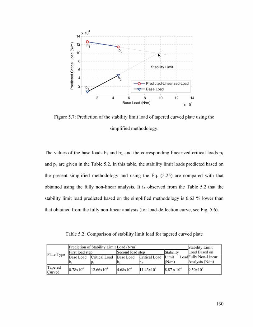
130

Figure 5.7: Prediction of the stability limit load of tapered curved plate using the

simplified methodology.

The values of the base loads b1 and b2, and the corresponding linearized critical loads p1

and p2 are given in the Table 5.2. In this table, the stability limit loads predicted based on

the present simplified methodology and using the Eq. (5.25) are compared with that

obtained using the fully non-linear analysis. It is observed from the Table 5.2 that the

stability limit load predicted based on the simplified methodology is 6.63 % lower than

that obtained from the fully non-linear analysis (for load-deflection curve, see Fig. 5.6).

Table 5.2: Comparison of stability limit load for tapered curved plate

Plate Type

Prediction of Stability Limit Load (N/m) Stability Limit Load Based on Fully Non-Linear Analysis (N/m)

First load step Second load step Stability Limit Load (N/m)

Base Load b1

Critical Load p1

Base Load b2

Critical Load p2

Tapered Curved 0.78x104 12.66x104 4.68x104 11.43x104 8.87 x 104 9.50x104

2 4 6 8 10 12 14

x 104

2

4

6

8

10

12

14x 104

Base Load (N/m)

Pre

dict

ed C

ritic

al L

oad

(N/m

)


Stability Limit

p1p2

b1

b2

131


The load carrying capability of the tapered curved plates is studied in the Ref. [116]

considering first-ply failure load. This type of failure analysis is considered to determine

whether a layer in the laminate has failed due to compressive loading before global

buckling occurs. Element SHELL99 is used for the analyses using ANSYS®. First-ply

failure analysis is carried out in the Ref. [116] using ANSYS® based on the 3-D version

of Tsai-Wu failure criterion. Material properties of composite material and epoxy are

given in the Tables 2.5 and 2.6 respectively.

Four different sizes of square tapered composite plates with the taper configuration of

Fig. 5.1 and made of NCT/301 graphite-epoxy composite material are considered. The

lay-up is [0/90]9s at the thick end and [0/90]3s at the thin end. The side length of the

square plate varies from 85.9 mm to 859.4 mm, plate thickness at the thick end (htk) is 4.5

mm and radius (R) of the plate is 500 mm. The clamped-clamped (C4-C4) boundary

conditions given in the Appendix D are considered. The side length of square plates

corresponding to various values of taper angles are given in the Table 5.3. The first-ply

failure loads are compared with the linear buckling and stability limit loads based on the

present simplified methodology. From this table, the following observations are made:

a) The tapered curved plates corresponding to the taper angles of 0.75 and 1.0

degrees will fail by first-ply failure before the linear global buckling (see Table

3.3). In the case of stability limit load, tapered plate corresponding to the taper

angle of 1.0 degree will fail by first-ply failure.

132

b) On the other hand, the plates corresponding to the taper angles of 0.1 and 0.50

degrees will not fail by first-ply failure if the linear buckling load is considered.

The plates corresponding to the taper angles of 0.1, 0.50 and 0.75 degrees will not

fail by first-ply failure if the stability limit load is considered. The maximum plate

size should be corresponding to the taper angle of 0.53 and 0.79 degrees for linear

buckling loads and stability limit loads respectively.

c) The critical length-to-height ratio (Ltap / htk) is to be 36 (see Fig. 3.2) and 24 (see

Fig. 5.8) for the linear buckling load and stability limit load respectively.

d) In terms of numerical values, the difference between the two loads (linear

buckling load and stability limit load) decreases with decrease of plate size. This

is so because the plate becomes stiffer with the decrease of plate size and the

stability limit load of stiff plate is closer to the bifurcation-buckling load (linear

buckling load).

e) The failed layers with numbers 2 and 3, respectively, are the second layer and the

third layer from the bottom at the thick end of the plates. All the tapered curved

plates failed at the thick end where the number of plies above or below the resin

pockets are at minimum.

Table 5.3: Comparison of linear buckling load, stability limit load and first-ply failure

load of tapered curved composite plates

Taper Angle in Degree


Linear Buckling Load [116]

(N/m)

Stability Limit Load Based on the Simplified Methodology (N/m)

First-ply Failure Load [116] (N/m)


0.10 0.8594 14.08 x104 8.87 x104 48.05 x104 1, 2 0.50 0.1719 40.05 x104 25.68 x104 42.00 x104 1, 2 0.75 0.1146 59.37 x104 42.55 x104 43.50 x104 9, 3 1.00 0.0859 79.48 x104 59.61 x104 45.60 x104 9, 3

* FEN and FLN denote the failed element number and failed layer number at first-ply failure.

133

Next, the tapered plates of the Table 5.3 are analyzed corresponding to different radii

using the same boundary condition (C4-C4), laminate configuration, and the material

properties of Tables 2.5 and 2.6. The critical sizes of the tapered curved plates are

determined corresponding to various radii. For the calculation of critical length-to-height

ratio, the same procedure is applied as that used in the previous case of the plate with the

radius of 500 mm. In the Fig. 5.8, the plot of radius versus critical length-to-height ratio

of tapered curved plates is given. In this figure, Ltap denotes the taper length and htk

denotes the thickness of the plate at the thick end. From Fig. 5.8, the following


a) The critical length-to-height ratio of the plate increases with the decrease of

radius. This is so because the stiffness of the tapered curved plate increases with

the decrease of radius. The critical length-to-height ratio varies non-linearly with

the radius. In the case of larger radius, shorter plate can be used under uni-axial

compression, which will not fail before global buckling.

b) The design limit for the tapered curved composite plates mentioned in the Table

5.3 corresponds to the shaded area of the Fig. 5.8. Beyond this limit, tapered

curved plate will not fail by ply failure before global buckling of the plate occurs.

Dark shaded area represents the design limit predicted by the present simplified

non-linear buckling (stability limit) analysis, and the dark and light shaded areas

together represent the design limit corresponding to the linear buckling analysis.

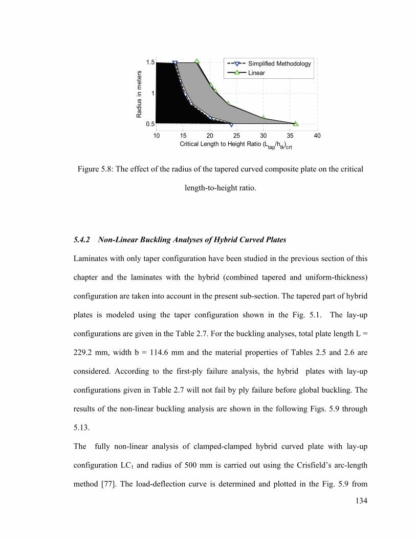
134

Figure 5.8: The effect of the radius of the tapered curved composite plate on the critical

length-to-height ratio.

5.4.2 Non-Linear Buckling Analyses of Hybrid Curved Plates

Laminates with only taper configuration have been studied in the previous section of this

chapter and the laminates with the hybrid (combined tapered and uniform-thickness)

configuration are taken into account in the present sub-section. The tapered part of hybrid

plates is modeled using the taper configuration shown in the Fig. 5.1. The lay-up

configurations are given in the Table 2.7. For the buckling analyses, total plate length L =

229.2 mm, width b = 114.6 mm and the material properties of Tables 2.5 and 2.6 are

considered. According to the first-ply failure analysis, the hybrid plates with lay-up

configurations given in Table 2.7 will not fail by ply failure before global buckling. The

results of the non-linear buckling analysis are shown in the following Figs. 5.9 through

5.13.

The fully non-linear analysis of clamped-clamped hybrid curved plate with lay-up

configuration LC1 and radius of 500 mm is carried out using the Crisfield’s arc-length

method [77]. The load-deflection curve is determined and plotted in the Fig. 5.9 from

10 15 20 25 30 35 40

0.5

1

1.5

Critical Length to Height Ratio (Ltap/htk)crtR

adiu

s in

met

ers

Simplified MethodologyLinear

135

which the stability limit load is calculated at the point where the transverse deflection

increased significantly with the small increment of compressive load and this value is to

be equal to 19.0x104 N/m.

Figure 5.9: Load-deflection curve for clamped hybrid curved plate

Alternatively, the stability limit load is calculated by linear interpolation using the present

simplified methodology. A linearized buckling analysis based on the pre-stress load (b1)

is performed, and an approximated critical load (p1) is obtained (see Fig. 5.10). Then a

suitable second base load (b2) is applied to the structure and another linearized buckling

analysis is performed to obtain a new predicted critical load (p2). Finally, extrapolation

from points (b1, p1) and (b2, p2) is made to find its intersection. The intersection point

corresponds to the stability limit load of the tapered curved plate.

The values of the base loads b1 and b2, and the corresponding linearized critical loads p1

and p2 are given in the Table 5.4. In this table, the stability limit load predicted using the

0 1 2 3

x 10-4

0

0.5

1

1.5

2

2.5

3

3.5x 105


Load

(N/m

)

Stability Limit

136

present simplified methodology is compared with that obtained using fully non-linear

analysis. It is observed from the Table 5.4, the stability limit load predicted based on

simplified methodology is 8.94 % lower than that obtained from fully non-linear analysis

(for the load-deflection curve, see Fig. 5.9).

Figure 5.10: Prediction of the stability limit load of hybrid curved plate using simplified

methodology.

Table 5.4: Comparison of the stability limit load for hybrid curved plate

Plate Type

Prediction of Stability Limit Load (N/m) Stability Limit Load Based on Fully Non-Linear Analysis (N/m)

First load step Second load step Stability Limit Load (N/m) Base Load

b1 Critical Load p1

Base Load b2

Critical Load p2

Hybrid Curved 1.0x104 20.6x104 5.0x104 19.95x104 17.3 x104 19.0x104

5.4.2.1 Influence of Radius-to-Thickness Ratio

Figs. 5.11 through 5.13 show the influence of the radius-to-thickness ratio on the

normalized stability limit and the normalized linear buckling load. The normalized

0.5 1 1.5 2 2.5

x 105

0.5

1

1.5

2

2.5x 105

Base Load (N/m)

Pre

dict

ed C

ritic

al L

oad

(N/m

)


Stability Limit

p1 p2

b1b2

137

stability limit loads corresponding to different radius-to-thickness ratio of hybrid curved

plates are calculated using simplified methodology based on Sander’s theory and these

normalized loads are compared with the linear buckling loads obtained using Ritz method

based on Classical Shell Theory (CST) and First-order shear deformation Shell Theory

(FST). In the Figs. 5.11 – 5.13, R denotes the radius, htk denotes the thickness of the plate

at thick end, crλ denotes the stability limit load or critical linear buckling load, Ltap

denotes the length of taper section and Ex” denotes the elastic modulus of the composite

material in the fiber direction. From Figs. 5.11 – 5.13, the following observations are

made:

a) All types of normalized loads decrease with the increase of radius-to-thickness

ratio.

b) The lowest and highest normalized loads are obtained using the simplified

methodology and CST-based Ritz solution respectively. In the case of CST-based

Ritz solution, shear strains are omitted which is the cause for higher buckling

loads compared to that obtained using the other two methods. The normalized

load using the simplified methodology is lower than that of the FST-based Ritz

solution. Because the equations for the strains of non-linear shell theory which is

linearized to calculate the stability limit load have more non-linear terms

compared to the linear shell theory.

c) Stability limit load of hybrid plates are strongly radius-to-thickness ratio

dependent.

138

d) The stability limit load diverges away from the linear buckling load with the

increase of radius-to-thickness ratio. This is so because the plate becomes more

flexible with the increase of radius.


clamped-clamped hybrid plate with lay-up configuration LC1.



100 150 200 250 300 3500.4

0.6

0.8

1

1.2

1.4

1.6

1.8

2


Nor

mal

ized

Buc

klin

g Lo

ad ( λ

cr*L

2 /Ex"

*htk3

)

Ritz-CST [Ref.111-112]Ritz-FST [Ref.116]Stability Limit Load

100 150 200 250 300 3500.4

0.6

0.8

1

1.2

1.4


Nor

mal

ized

Buc

klin

g Lo

ad ( λ

cr*L

2 /Ex"

*htk3

)


139



5.5 CONCLUSIONS

In the present chapter, fully non-linear and linearized buckling analyses have been carried

out using finite element method based on two well known first-order shallow shell

theories, namely, Donnel’s, and Sander’s theories. Three types of composite plates, that

are, uniform-thickness, tapered and hybrid plates are considered under uni-axial

compressive load. A detailed parametric study of curved (tapered and hybrid ) plates has

been conducted that includes the influences of taper angle, critical length-to-height ratio,

radius, radius-to-thickness ratio and geometric parameters of the plates on the buckling

load. The conclusions listed herein, are based on all the numerical results presented.

100 150 200 250 300 3500.4

0.6

0.8

1

1.2

1.4

1.6

1.8


Nor

mal

ized

Buc

klin

g Lo

ad ( λ

cr*L

2 /Ex"

*htk3

)


140

a) Any of the above mentioned shell theories can be used for the buckling analysis of

flat or tapered curved plates. However, the Sander’s shell theory provides the most

conservative results.

b) Stability limit load calculated based on the simplified methodology has agreement

with that of the fully non-linear analysis. The present simplified methodology

consumes reasonably shorter computational time compared to the standard fully

non-linear analysis.

c) The moderately thick and tapered curved composite plates may fail by ply failure

before global buckling. Therefore, the tapered curved plate should be larger than

the corresponding critical size. The critical size depends on both the radius and

taper angle of the plate.

d) Stability limit load of hybrid plate depends strongly on the radius-to-thickness

ratio.

141

Chapter 6

Conclusions, Contributions, and Future Work

6.1 CONCLUDING REMARKS

The objective of the present thesis work is to investigate the compressive response of

shallow curved composite plates with longitudinal internal ply-drop-off configurations.

For this purpose, three types of analyses, namely, global buckling (linear and non-linear),

first-ply failure, and delamination failure analyses are considered. Three types of tapered

plates (taper configurations A and B, and a hybrid configuration) and three types of lay-

up configurations (LC1, LC2 and LC3) are investigated.

Linear global buckling is carried out using Classical Shell Theory (CST) based on Ritz

method and using First-order shear deformation Shell Theory (FST) based on the Ritz

method and Finite Element Method (FEM). The classical linear buckling analysis is

carried out based on eight well-known classical shallow shell theories, namely Donnell’s,

Love’s, Mushtari’s, Timoshenko’s, Vlasov’s, Sander’s, Koiter’s and Novozhilov’s

theories. The linear buckling analysis is also carried out based on six well-established

first-order shear deformation shell theories, that are, Donnell’s, Moreley’s, Love’s, Loo’s,

Koiter’s and Sander’s theories. The Ritz method is used to solve both of the CST and

FST based linear buckling problems. A nine-node tapered curved composite finite

element is developed based on the above mentioned six first-order shear deformation

shell theories. In the case of different shell theories, the corresponding critical buckling

loads are calculated and the most conservative value is obtained.

142

Linear buckling analysis is insufficient to take into account the effect of large deflections

on the buckling loads of structural components. This effect can only be considered in the

non-linear buckling analysis. However, very large number of load steps is required to

determine the buckling load based on the non-linear analysis in which the stability limit

load is calculated from the non-linear load-deflection curve. In the present thesis work, a

simplified methodology is developed to predict the stability limit load that requires the

consideration of only two load steps. The stability limit loads of the tapered curved plates

are calculated using this simplified methodology.

The strength characteristics and load carrying capability of the tapered curved plates are

investigated considering the first-ply failure and delamination failure analyses using

ANSYS®. First-ply failure analysis is carried out based on the 3-D version of Tsai-Wu

failure criterion. The initiation of delamination, if any, is dictated by the transverse

interlaminar stresses developed under compressive load. The interlaminar transverse

shear stresses in shell element are calculated based on the assumption that no shear is

carried at the top and bottom surfaces of the element. These interlaminar shear stresses

are only computed in the interior of the element and are computed using equilibrium

requirements.

Based on the failure and buckling analyses, the critical sizes and parameters of the

tapered curved plates that will not fail before global buckling are determined. Parametric

studies that encompass the effects of boundary conditions, stacking sequence, taper

configurations, radius and other geometric parameters of the plates are conducted.

143

Based on the present study, the following main concluding remarks are made:

a) The buckling results based on different classical shell theories are close to each

other but the Novozhilov’s shell theory provides the most conservative result.

b) Any of the previously mentioned first-order shear deformation shell theories can be

used for the buckling analysis of uniform or tapered curved plates. But the Sander’s

and the Koiter’s shell theories provide the most conservative result.

c) The moderately-thick and tapered curved composite plates can also fail by first-ply

failure before global buckling. Therefore the dimensions of tapered curved plate

should be larger than the corresponding critical size. The critical sizes depend on

both radius and stacking sequence of the plates. Such critical sizes have been

determined in the present work.

d) The tapered flat plate is more flexible than uniform flat plate, but the tapered

curved plate provides a better design option in terms of saving the material without

any compromise of the strength.

e) Uniaxial compressive strength can be increased significantly by making the tapered

plate into a curved one and a considerable amount of material can also be saved.

f) The critical buckling loads of all lay-up configurations are considerably influenced

by the stiffness ratio (Ex”/Ey”) of the ply material.

g) Classical shell theory can be used to calculate with reasonable accuracy the critical

buckling loads of moderately-long plates for which Ltap/R > 0.35. The first-order

shear deformation shell theory should be used for the calculation of critical

buckling loads of shorter plates for which Ltap/R < 0.35.

144

h) The normalized buckling load is more dependent on length-to-radius ratio (Ltap/R)

than the taper configuration.

i) The buckling behavior of all the lay-up configurations are both radius-to-thickness

ratio (R/htk) and boundary condition dependent. At higher values of radius, lay-up

configurations LC3, LC1 and LC2 become the strongest, moderate and weakest

laminates respectively.

j) Stability limit load calculated based on the simplified methodology has agreement

with that of the fully non-linear analysis. The present simplified methodology



6.2 CONTRIBUTIONS

The remarkable contributions made in this thesis are summarized below:

1) One of the important contributions of the present thesis is a systematic and

thorough study of the compressive response of the tapered curved composite

plates. The tapered curved plate provides a better design option in terms of saving

the material without any compromise of the strength. The cost of the engineering

products can be minimized by reducing the weight of the products. According to

Bombardier [119], the extra cost of $41,000 to 69,000 USD per year per aircraft is

needed for the extra Operating Empty Weight (OWE) of 500 kg of a regional jet.

2) The second most important contribution is the present simplified methodology that



145

3) The critical sizes and parameters of the tapered curved plates that will not fail by

first-ply failure and delamination failure before global buckling are determined.

This contribution is made for design purpose.

4) To apply the first-order shear deformation shell theories to analyze the tapered

plates, an appropriate set of shear correction factors have been determined.

6.3 RECOMMENDATIONS

The following recommendations for further study can be considered:

1) A low velocity transverse impact on a composite plate may cause internal

delaminations, which has not been considered in the present work. Therefore,

Compression After Impact (CAI) of the tapered curved plates can be considered in

the future work.

2) The post-buckling response of tapered curved composite plates including

progressive failure of the laminate under compressive and shear loadings.

3) To quantify the effect of stochastic variability in the material properties on the

progressive failure.

4) The dynamic buckling analysis of the tapered curved composite plates.

146

APPENDIX A

Boundary Conditions for Classical Shell Theory

S3: at x=0, L u ≠ dw/dx ≠ 0; w = v = Nxx = Mxx = 0

)sin(LxmWm π=

)sin(

LxmVm π=

)cos(

LxmU m π=

at y=0, b v≠ dw/dy ≠ 0; w = u = Myy = Nyy = 0

)sin(bynWn π=

)cos(

bynVn π=

)sin(

bynU n π=

(A1)

S4: at x=0, L dw/dx ≠ 0; w = v = u = Mxx = 0

)sin(LxmWm π=

)sin(LxmVm π=

)sin(LxmU m π=

at y=0, b dw/dy ≠ 0; w = u = v = Myy = 0

)sin(bynWn π=

)sin(bynVn π=

)sin(bynU n π=

(A2)

C3: at x=0, L u ≠ Mxx ≠ 0; w = v = Nxx = dw/dx = 0

⎟⎠

⎞⎜⎝

⎛ −−⎟⎠

⎞⎜⎝

⎛ −=L

xL

xL

xL

xW ii

iii

mλλ

γλλ

sinhsincoshcos

Vm =Wm;

)cos(LxmU m π=

at y=0, b v ≠ Myy ≠ 0; w = u = dw/dy = Nyy = 0

⎟⎠

⎞⎜⎝

⎛ −−⎟⎠

⎞⎜⎝

⎛ −=b

yb

yb

yb

yW ii

iii

nλλ

γλλ

sinhsincoshcos

)cos(bynV n π=

Un=Wn

(A3)

C4: at x=0, L Mxx ≠ 0; w = v = dw/dx = 0

⎟⎠

⎞⎜⎝

⎛−−⎟

⎠

⎞⎜⎝

⎛−=

Lx

Lx

Lx

Lx

W iii

iim

λλγ

λλsinhsincoshcos

Vm =Wm;

dxdW

U mm = ; u = 0 at x = L

)cos(LxmU m π= ; u ≠ 0 at x = 0

at y=0, b Myy ≠ 0; w = u = v = dw/dy = 0

⎟⎠

⎞⎜⎝

⎛ −−⎟⎠

⎞⎜⎝

⎛ −=b

yb

yb

yb

yW ii

iii

nλλ

γλλ

sinhsincoshcos

dydW

V nn =

Un = Wn

(A4)

In general, the displacement functions are expressed in the Equations (2.17) through

(2.19) and Um, Un, Vm, Vn, Wm and Wn are selected from the above expressions for

different boundary conditions. L and b are the length and width of the plate respectively;

Nij and Mij are the resultant force and moment respectively, where i, j = x, y. The values

147

of Lamda, λi and Gama, γi can be found in Bertholate [103]. Si and Ci are the simply

supported and clamped boundary conditions respectively with i= 3, 4.

System Equations of Classical Shallow Shell Theories

For balanced symmetric laminate, Bij=0 and A16=A26=0; applying these conditions to the

equations (2.26), the following expressions of stIJL and st

IJG are obtained, where s, t = 1,

2, 3:

⎪⎭

⎪⎬⎫

⎭⎬⎫

⎟⎠⎞

⎜⎝⎛++

⎪⎩

⎪⎨⎧

⎩⎨⎧

=

∫∫∫∫

∑∑ ∫∫∑∑= == =

dydy

dUdy

dUdxUURcDdyUUdx

dxdU

dxdUA

dydy

dUdy

dUdxUUAL

bjn

L

im

b

jnim

L

M

i

N

j

bjn

L

im

M

m

N

nIJ

00

24

6600

11

1 1 0066

1 1

11

(A5)

⎪⎭

⎪⎬⎫

⎭⎬⎫

+

+−

⎪⎩

⎪⎨⎧

⎩⎨⎧−=

∫∫

∫∫∫∫

∑ ∑ ∫∫∑∑= == =

dydy

dVUdxV

dxdU

A

dyVdy

dUdx

dxdV

UAdyVdy

dUdx

dxdV

UccRD

dydy

dVdy

dUdxVUc

Rc

DL

bj

nim

L

b

jni

m

Lb

jni

m

L

M

i

N

j

bjn

L

im

M

m

N

nIJ

0012

0066

043

02

66

1 1 0042

226

1 1

12

(A6)

⎪⎭

⎪⎬⎫

⎭⎬⎫

++

++

⎪⎩

⎪⎨⎧

⎪⎩

⎪⎨⎧

=

∫∫∫∫

∫∫∫∫

∑∑ ∫∫∑∑= == =

dyWdy

dUdxdx

WdUcR

DdyWUdxWdx

dUR

A

dyWdy

dUdxWUcRcDdy

dydW

dydUdx

dxdWUc

RD

dydy

Wddy

dUdxWUcR

DL

b

jni

m

Lb

jnim

L

b

jn

im

Lbjni

m

L

M

i

N

j

bjn

L

im

M

m

N

nIJ

02

2

40

16

00

12

043

1

026

04

0

66

1 1 02

2

04

26

1 1

13

2

(A7)

⎪⎭

⎪⎬⎫

⎭⎬⎫

+⎟⎠⎞

⎜⎝⎛+

++

⎟⎠⎞

⎜⎝⎛+

⎪⎩

⎪⎨⎧

⎩⎨⎧

=

∫∫∫∫

∫∫∫∫

∫∫∑∑ ∫∫∑∑= == =

dyVdy

dVdxdxdVVc

RcDdy

dydV

dydVdxVV

RcD

dydy

dVVdxV

dxdVc

RcDdyVVdx

dxdV

dxdVA

dyVVdxdxdV

dxdV

RcDdy

dydV

dydVdxVVAL

b

jni

m

Lbjn

im

L

bj

nim

Lb

jnim

L

b

jn

Lim

M

i

N

j

bjn

L

im

M

m

N

nIJ

032

2

026

0

22

022

032

2

026

0066

00

23

661 1 00

221 1

22

(A8)

148

dyWdy

dVdxWV

RAdyWVdx

dxWd

dxdV

Rc

D

dyWVdxWdx

dVc

RcDdy

dydW

Vdxdx

dWdx

dVc

RD

L

b

jn

im

Lb

jnim

L

b

jn

L

im

M

i

N

j

bj

n

Lim

M

m

N

nIJ

∫∫∫∫

∫∫∑∑ ∫∫∑∑

+−

−⎪⎩

⎪⎨⎧

⎩⎨⎧−=

= == =

00

22

02

23

016

0033

126

1 1 003

66

1 1

23 2

⎪⎭

⎪⎬⎫

⎭⎬⎫

−

−−

−−

∫∫

∫∫∫∫

∫∫∫∫

dyWdy

dVdx

dxWd

VRcD

dydy

Wddy

dVdxWV

Rc

DdyWdy

dVdxWVc

Rc

D

dydy

dWdy

dVdx

dxdW

VRc

Ddydy

WdVdxW

dxdV

Rc

D

b

jni

m

L

bjn

im

Lb

jn

im

L

bjni

m

Lbj

nim

L

02

22

012

02

2

0

222

023

1

022

00

226

02

23

026 2

(A9)

⎪⎭

⎪⎬⎫

⎪⎩

⎪⎨⎧

⎪⎩

⎪⎨⎧

⎭⎬⎫

= ∑ ∑ ∫∫∑ ∑= == =

M

i

N

j

b

jn

Lim

M

m

N

nIJ dyVVdx

dxdV

dxdV

G1 1 001 1

22 (A10)

⎪⎭

⎪⎬⎫

⎪⎩

⎪⎨⎧

⎪⎩

⎪⎨⎧

⎭⎬⎫

= ∑ ∑ ∫∫∑ ∑= == =

M

i

N

j

b

jn

Lim

M

m

N

nIJ dyWWdx

dxdW

dxdW

G1 1 001 1

23 (A11)

⎥⎦

⎤⎢⎣

⎡++

++

⎢⎢⎣

⎡⎥⎦

⎤++

+⎪⎩

⎪⎨⎧

⎩⎨⎧

=

∫∫∫∫

∫∫∫∫

∫∫∫∫

∫∫∑∑ ∫∫∑∑= == =

dydy

dWWdx

dxdW

dxWdDdy

dyWdWdxWW

RcD

dyWdy

dWdxWdx

dWRcDdyW

dydWdx

dxWd

dxdWD

dydy

dWdy

Wddxdx

dWWDdyWdy

WddxWWRcD

dyWWdxWdx

WdRcDdy

dydW

Wdxdx

dWWRcDL

bj

n

Lim

bi

n

L

im

b

jn

L

im

b

jn

Lim

bjn

Li

mj

bn

L

im

b

jn

L

im

M

i

N

j

bj

n

Li

m

M

m

N

nIJ

002

2

160

2

2

02

122

002

126

002

2

16

02

2

026

02

2

02

122

002

2

21

121 1 00

21

261 1

33

2

22

2

2

dydy

dWdy

dWdx

dxdW

dxdW

Ddydx

Wddx

dWdxW

dxdW

D

dydy

WdWdxW

dxWd

DdyWWdxWWRcD

bjn

Lim

bjn

i

Lm

bj

n

L

im

b

jn

L

im

∫∫∫∫

∫∫∫∫

++

++

0066

02

2

026

02

2

02

2

1200

4

21

22

42

(A12)

⎪⎭

⎪⎬⎫

⎪⎭

⎪⎬⎫

+

++

++

∫∫

∫∫∫∫

∫∫∫∫

dydy

Wddy

WddxWWD

dyWdy

Wddxdx

WdWDdyWWdxWWRA

dyWWdxdx

WddxWdDdyWWdx

dxWdW

RcD

bjn

L

im

b

jn

Li

m

b

jn

L

im

b

jn

Lim

b

jn

Li

m

02

2

2

2

022

02

2

02

2

1200

222

002

2

2

2

1100

2

2

21

12

The respective values of c1, c2, c3 and c4 are given in the section of formulation.

149

APPENDIX B

Boundary Conditions for First-order Shear Deformation Shell Theory

S3: at x = 0, L w = Mxx = yϕ = Nxx = v = 0

)sin(LxmWm π=

)sin(LxmVm π=

)cos(LxmU m π=

)cos()(Lxmmx πϕ =

)sin()(

Lxmmy πϕ =

at y = 0, b w = Myy = xϕ

= Nyy = u = 0

)sin(bynWn π=

)cos(bynVn π=

)sin(bynU n π=

)sin()(

bxnnx πϕ =

)cos()(bxnny πϕ =

(B1)

S4:

at x = 0, L w = Mxx = yϕ = u = v = 0

)sin(LxmWm π=

)sin(LxmVm π=

)sin(LxmU m π=

)cos()(Lxmmx πϕ =

)sin()(

Lxmmy πϕ =

at y = 0, b w = Myy = xϕ

= u = v = 0

)sin(bynWn π=

)sin(bynVn π=

)sin(bynUn π=

)sin()(

bxnnx πϕ =

)cos()(bxnny πϕ =

(B2)

C3:

at x = 0, L w = xϕ = yϕ = Nxx = v = 0

⎟⎠⎞

⎜⎝⎛ −−⎟

⎠⎞

⎜⎝⎛ −=

Lx

Lx

Lx

LxW ii

iii

mλλγλλ sinhsincoshcos

)sin(LxmVm π=

)cos(LxmU m π=

)sin()(Lxmmx πϕ =

)sin()(

Lxmmy πϕ =

at y = 0, b w = xϕ = yϕ

= Nyy = u = 0

⎟⎠⎞

⎜⎝⎛ −−⎟

⎠⎞

⎜⎝⎛ −=

by

by

by

byW ii

iii

nλλ

γλλ sinhsincoshcos

)cos(bynVn π=

)sin(bynUn π=

)sin()(

bxnnx πϕ =

)sin()(bxnny πϕ =

(B3)

150

C4: at x = 0, L w = xϕ = yϕ = v = 0

⎟⎠⎞

⎜⎝⎛ −−⎟

⎠⎞

⎜⎝⎛ −=

Lx

Lx

Lx

LxW ii

iii

mλλγλλ sinhsincoshcos

)sin(LxmVm π=

)sin(LxmU m π=

; u = 0 at x = L

)cos(LxmU m π=

; u ≠ 0 at x = 0

)sin()(

Lxmmx πϕ =

,)sin()(

Lxmmy πϕ =

at y = 0, b w = xϕ = yϕ = u = v = 0

⎟⎠⎞

⎜⎝⎛ −−⎟

⎠⎞

⎜⎝⎛ −=

by

by

by

byW ii

iii

nλλ

γλλ sinhsincoshcos

)sin(bynVn π=

)sin(bynUn π=

)sin()(

bxnnx πϕ =

)sin()(bxnny πϕ =

(B4)

In general, the displacement functions are expressed as in the Equations (3.15) through

(3.19) and functions Um, Un, Vm, Vn, Wm, Wn, xϕ and yϕ are selected from the above

expressions for different boundary conditions. L and b are the length and width of the

plate respectively; Nij and Mij are the resultant force and moment respectively, where i, j

= x, y. The values of λi and γi can be found in Bertholet [103]. Si and Ci denote the

simply-supported and clamped boundary conditions respectively, where i = 3, 4.

Different Edge Conditions of the Curved Plates

C4

C4

C4

C4 S4

S4

S4

S4 C3

S3

S3

C3

Clamped-Clamped (C4-C4) Simply-Supported (S4-S4) Clamped-Simply Supported (C3-S3)

The details about the boundary conditions where S3, S4, C3 and C4 are, respectively,

given by the Eqs. (B1) through (B4).

System Equations of First-order Shear Deformation Shell Theory For balanced symmetric laminate, B11= B12= B16= B22= B26= B66=0, and A16=A26=0;

applying these conditions to the Eq. (3.25), the following expressions for stIJL are

obtained:

151

⎪⎭

⎪⎬⎫

⎭⎬⎫

⎟⎠⎞

⎜⎝⎛++

⎪⎩

⎪⎨⎧

⎩⎨⎧

=

∫∫∫∫

∑ ∑ ∫∫∑ ∑= == =

dydy

dUdy

dUdxUURcDdyUUdx

dxdU

dxdUA

dydy

dUdy

dUdxUUAL

bjn

L

im

b

jnim

L

M

i

N

j

bjn

L

im

M

m

N

nIJ

00

21

6600

11

1 1 0066

1 1

11

4/1

(B5)

⎪⎭

⎪⎬⎫

⎭⎬⎫

−+

++

−⎪⎩

⎪⎨⎧

⎪⎩

⎪⎨⎧

⎟⎠⎞

⎜⎝⎛−=

∫∫∫∫

∫∫∫∫

∫∫∑∑ ∫∫∑∑= == =

dyVdy

dUdxVURcAdyV

dydUdxVU

RccB

dydy

dVUdxV

dxdUAdyV

dydUdx

dxdVUA

dyVUdxVdx

dUARcdyV

dydUdx

dxdVUD

RcL

b

jn

L

im

b

jn

im

L

bj

nim

Lb

jni

m

L

b

jnim

LM

i

N

j

b

jn

Li

m

M

m

N

nIJ

00

246

0221

046

0012

0066

0014

2

1 1 0066

21

1 1

12

21

41

(B6)

⎪⎭

⎪⎬⎫

⎭⎬⎫

−

−+

++

+⎪⎩

⎪⎨⎧

⎩⎨⎧

=

∫∫

∫∫∫∫

∫∫∫∫

∫∫∑∑ ∫∫∑∑= == =

dydy

dWdy

dUdxWURcB

dyWdy

dUdxdx

dWURcBdyWUdxW

dxdU

RA

dydy

dWdy

dUdxWUAdydy

dWUdxW

dxdUA

dyWdy

dUdxdx

dWUAdyWUdxdx

dWdx

dUAL

bjn

L

im

b

jni

m

Lb

jnim

L

bjn

im

Lbj

nim

L

b

jni

m

LM

i

N

j

b

jn

Lim

M

m

N

nIJ

00

146

0

1

056

0012

0046

0014

0056

1 1 0015

1 1

13

21

211

(B7)

where c1 and c2 are the tracer coefficients used to express the strain and curvature fields

that correspond to different shell theories. In a similar manner, the equations for rest of

the coefficients stIJL (s, t = 1, 2, 3, 4, 5) can be written.

stIJG can be expressed as:

⎪⎭

⎪⎬⎫

⎪⎩

⎪⎨⎧

⎪⎩

⎪⎨⎧

⎭⎬⎫

= ∑∑ ∫∫∑∑= == =

M

i

N

j

b

jn

Lim

M

m

N

nIJ dyVVdx

dxdV

dxdVG

1 1 001 1

22 (B8)

⎪⎭

⎪⎬⎫

⎪⎩

⎪⎨⎧

⎪⎩

⎪⎨⎧

⎭⎬⎫

= ∑∑ ∫∫∑∑= == =

M

i

N

j

b

jn

Lim

M

m

N

nIJ dyWWdx

dxdW

dxdW

G1 1 001 1

33 (B9)

where L and b are the length and the width of a plate respectively and L denotes the total

length of a plate, that is, L= Ltap for taper configurations A and B, and L = L for hybrid

configuration (see Fig. 1.4).

152

APPENDIX C

Shape Functions for the Nine-node Lagrange Element

221 b)/b-y)(b

21-y( )/-x)(

21-x4( LLLN =

22

2 b)/b-y(y )/-x)(21-x-8( LLLN =

(C1)

223 b)/b

21-y(y )/-x)(

21-x4( LLLN =

22

4 b)/b-y)(b21-y( )/-x(x-8 LLN =

225 b)/b-y(y )/-x(x16 LLN =

226 b)/b

21-y(y )/-x(x-8 LLN =

22

7 b)/b-yb)(21-y()/

21-x(x4 LLN =

22

8 b)/b-y(y )/21-x(x-8 LLN =

229 b)/b

21-y(y )/

21-x(x4 LLN =

where L and b are the length and the width of an element respectively with respect to

local coordinates; and is the set of local coordinates.

[ ]

⎥⎥⎥⎥⎥⎥⎥⎥⎥⎥⎥⎥⎥⎥⎥⎥⎥⎥⎥

⎦

⎤

⎢⎢⎢⎢⎢⎢⎢⎢⎢⎢⎢⎢⎢⎢⎢⎢⎢⎢⎢

⎣

⎡

−

−

=

000

00

022

0000

0000

000

000

0000

2

11

ii

ii

i

iiii

i

i

ii

ii

i

iL

Ndx

dN

NdydNN

Rc

dxdN

dydN

dxdN

Rc

dydN

Rc

dydN

dxdN

dxdN

dydN

RN

dydN

dxdN

B

(C2)

[ ]

⎥⎥⎥⎥⎥⎥

⎦

⎤

⎢⎢⎢⎢⎢⎢

⎣

⎡

=

0000000000

00000000000000

dxdN

g iiL

(C3)

153


S3:

at x = 0, L w = Mxx = yϕ = Nxx = vo = 0 at y = 0, b w = Myy = xϕ = Nyy = uo = 0

(C4)

S4:

at x = 0, L w = Mxx = yϕ = uo = vo = 0 at y = 0, b w = Myy = xϕ = uo= vo = 0

(C5)

C3:

at x = 0, L w = xϕ = yϕ = Nxx = vo = 0 at y = 0, b w = xϕ = yϕ = Nyy = uo= 0

(C6)

C4:

at x = 0, L w = xϕ = yϕ = uo = vo = 0 at y = 0, b w = xϕ = yϕ = uo = vo = 0

(C7)

where (uo, vo, wo) constitute the mid-plane displacement field that refers to the global

coordinate system (x, y, z) as shown in Fig. 2.1; L and b are the length and width of a

plate respectively; Nij and Mij are the resultant forces and moments respectively, where i,

j = x, y.

Different Edge Conditions of the Curved Plates

C4

C4

C4

C4 S4

S4

S4

S4 C3

S3

S3

C3

Clamped-Clamped (C4-C4) Simply-Supported (S4-S4) Clamped-Simply Supported (C3-S3)

The details about the boundary conditions S3, S4, C3 and C4 are, respectively, given by

the Eqs. (C4) through (C7).

154

Calculation of the Weight Savings and the Gain of Strengths

To calculate the weight of a tapered laminate, the laminate is divided into several

segments based on the horizontal distribution of resin pockets. For example, taper

configuration A has only one segment but the taper configuration B has three segments.

The weight of all the segments is combined to get the weight of the laminate. The resin

pocket is considered (imagined) to be made up of layers of isotropic resin material and

the height of the resin pocket is equivalent to the number of drop-off plies.

The weight of the uniform flat laminate which is to be made into the tapered one is:

∑=

××××+×+××=N

ncprpcrrul btLNCPNURPPDOnW

1])([ ρρρ

(C8)

The weight of the tapered flat laminate can be expressed as:

∑ ××××+×+×××= ])([ 21 btLNCPNURPDOPnW cprpcrrtl ρρρ

(C9)

The weight of the tapered curved laminate can be expressed as:

∑ ×××××+×+×××= ])([ 21 ζρρρ RtLNCPNURPDOPnW cprpcrrtcl

(C10)

where ‘n’ denotes the number of segments, ‘PDO’ denotes the plies to be dropped-off,

‘DOP’ denotes the dropped-off plies, rρ denotes the density of resin, ‘NURP’ denotes the

number of uniform (imagined) resin plies, ‘NCP’ denotes the number of composite plies,

cρ denotes density of composite, Lrp denotes the length of the resin pocket, tcp denotes

the thickness of the composite plies, ‘b’ denotes the width of the flat plate, ‘R’ denotes

the radius of the curved plate, and ‘ζ ’ denotes the center angle of the curved plate.

The properties mentioned in the Eqs. (C8) and (C9) for the plate with one segment used

in the Fig. 4.6 are:

n = 1, PDO = 18, rρ = 1050 kg/m3, NURP = 6, NCP = 12, cρ = 1480 kg/m3, Lrp = 0.8594

m, tcp = 0.000125 m and b = 0.8594 m.

Therefore, the weight of the uniform flat plate corresponding to the point ‘P’ in the Fig.

4.6 is:

155

8594.0000125.8594.0)14801210506105018( ××××+×+×=PW

96.3=PW Kg (C11)

And the weight of the tapered plate corresponding to the point ‘Q’ in the Fig. 4.6 is:

8594.000125.8594.)148012105061050182/1( ××××+×+××=QW

09.3=QW Kg (C12)

The weight savings of the tapered plate with respect to the uniform plate is expressed as:

%100/)( ×−= PQPs WWWW (C13)

From the Eqs. (C11) through (C13), the weight savings of the plate used in the Fig. 4.6

with 18 drop-off plies is 21.96 %.

The gain of strength of a curved tapered plate with respect to a flat tapered plate can be

expressed as:

%100/)( ×−= RQRs SSSG (C14)

From the Eq. (C14), the gain of strength of the plate used in the Fig. 4.6 with 18 drop-off

plies is 82.47 %.

APPENDIX D

Strain-Nodal Displacement Matrix

[ ]

⎥⎥⎥⎥⎥⎥⎥⎥⎥⎥⎥⎥⎥⎥⎥⎥⎥⎥⎥⎥

⎦

⎤

⎢⎢⎢⎢⎢⎢⎢⎢⎢⎢⎢⎢⎢⎢⎢⎢⎢⎢⎢⎢

⎣

⎡

−

=

000

00

000

0000

0000

000

000

0000

1

ii

ii

i

ii

i

i

ii

ii

i

iL

Ndx

dN

Ndy

dNN

Rc

dxdN

dydN

dydN

dxdN

dxdN

dydN

RN

dydN

dxdN

B

(D1)

156

Matrices Required to Calculate

[ ]

⎥⎥⎥⎥⎥⎥⎥⎥⎥⎥⎥⎥⎥⎥

⎦

⎤

⎢⎢⎢⎢⎢⎢⎢⎢⎢⎢⎢⎢⎢⎢

⎣

⎡

⎟⎟⎠

⎞⎜⎜⎝

⎛−−

⎟⎟⎠

⎞⎜⎜⎝

⎛−⎟⎟

⎠

⎞⎜⎜⎝

⎛−−

=

000000000000000

0

00

1

11

dxdw

Rvc

dydw

dxdw

Rvc

dydw

Rvc

dydw

dxdw

Hoooo

oooo

o

(D2)

[ ]

⎥⎥⎥⎥⎥⎥

⎦

⎤

⎢⎢⎢⎢⎢⎢

⎣

⎡

=

0000

0000

0000 1

dydNdxdN

RNc

S

i

i

i

(D3)

Matrices Required to Calculate

[ ]⎥⎥⎥

⎦

⎤

⎢⎢⎢

⎣

⎡

−−

−−=

232

313

232

LLL

LLL

LLL

L

NNNNNNNNN

N (D4)

[ ]⎥⎥⎥

⎦

⎤

⎢⎢⎢

⎣

⎡

−−

−−=

232

313

232

NNN

NNN

NNN

N

NNNNNNNNN

N (D5)

{ } { } [ ] { } 1888'

82118 ........,, ××× == Lt

LLLLi ENNNN ε (D6)

{ } { } [ ] { } 1888'

82118 ........,, ××× == Nt

NNNNi ENNNN ε (D7)

157


For first-order shear deformation shell theory, the BCs of clamped-clamped (C4-C4)

plate are mentioned below:

at x = 0 w = xϕ = yϕ = uo = vo = 0 at x = L w = xϕ = yϕ = vo = 0; uo ≠ 0 at y = 0, b w = xϕ = yϕ = uo = vo = 0

(D8)

where (uo, vo, wo) denotes the mid-plane displacement field that refers to the global

coordinate system (x, y, z) as shown in Fig. 2.1; L and b are the length and width of the

plate respectively; Nij and Mij are the resultant force and moment respectively, where i, j

= x, y.

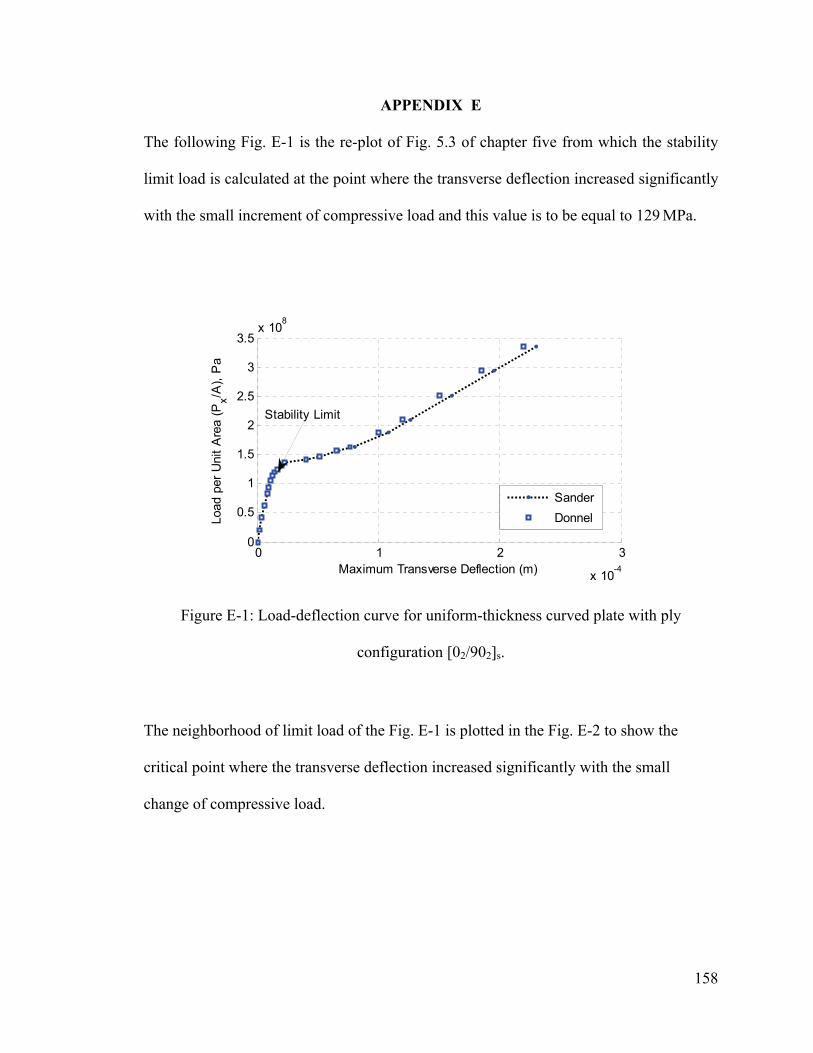
158

APPENDIX E

The following Fig. E-1 is the re-plot of Fig. 5.3 of chapter five from which the stability

limit load is calculated at the point where the transverse deflection increased significantly

with the small increment of compressive load and this value is to be equal to 129 MPa.

Figure E-1: Load-deflection curve for uniform-thickness curved plate with ply


The neighborhood of limit load of the Fig. E-1 is plotted in the Fig. E-2 to show the

critical point where the transverse deflection increased significantly with the small

change of compressive load.

0 1 2 3

x 10-4

0

0.5

1

1.5

2

2.5

3

3.5x 108


Load

per

Uni

t Are

a (P

x/A),

Pa

SanderDonnel

Stability Limit

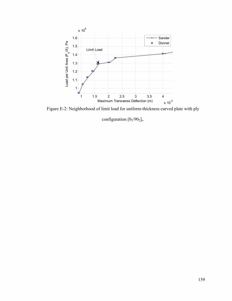
159

Figure E-2: Neighborhood of limit load for uniform-thickness curved plate with ply


1 1.5 2 2.5 3 3.5 4

x 10-5

1

1.1

1.2

1.3

1.4

1.5

1.6

x 108


Load

per

Uni

t Are

a (P

x/A),

Pa

SanderDonnel

Limit Load

160

ACKNOWLEDGEMENT

The author of the present thesis and the supervisor would like to acknowledge the support

provided for the present work by the Natural Sciences and Engineering Research Council

of Canada (NSERC) and Concordia University.

161

REFERENCES

1. He, K., Hoa, S. V. and Ganesan, R., “The Study of Tapered Laminated Composite

Structures: A Review”, Composites Science and Technology, Vol. 60, 2000, pp.

2643-2657.

2. Curry, J. M., Johnson, E. R. and Starnes Jr., J. H., “Effect of Dropped Plies on the

Strength of Graphite-epoxy Laminates”, AIAA Journal, Vol. 30(2), 1992, pp. 449-

456.

3. Hoa, S. V., Du, B. L. and Vu-Khanh, T., “Interlaminar Stresses in Tapered

Laminates”, Polymer Composites, Vol. 9(5), 1988, pp. 337-344.

4. Daoust, J. and Hoa, S. V., “Parameters Affecting Interlaminar Stresses in Tapered

Laminates Under Static Loading Conditions”, Polymer Composites, Vol. 10(5),

1989, pp. 374-83.

5. Llanos, A. S. and Vizzini, A. J., “The Effect of Film Adhensive on the

Delamination Strength of Tapered Composites”, Journal of Composite Materials,

Vol. 26(13), 1992, pp. 1968-1983.

6. Thomas, D. M. and Webber, P. H., “A Design Study into the Delamination

Behavior of Tapered Composites”, Composite Structures, Vol. 27, 1994, pp. 379-

88.

7. Piskunov, V. G. and Sipetov, V. S., “Calculation of Tapered Laminated Shells

Consisting of Anisotropic Composite Materials for Static and Thermal Loads”,

Kiev Highway Institute, Translated from Problemy Prochnosti, No. 10, October

1987, pp. 79-82.

162

8. Kee, Y. and Kim, J., “Vibration Characteristics of Initially Twisted Rotating Shell

Type Composite Blades”, Composite Structures, Vol. 64, 2004, pp. 151-159.

9. Lars, A. S. and Eggwertz, S., “Shell stability handbook”, Elsevier Science

Publishers Ltd., London, 1992.

10. Lorenz, R., “Achsensymetrische Verzerrungen in Dunnwandigen Holzylindern”,

Zeitschrift VDI, Bd 52, S 1706-1713, 1908, (Cross referenced from many other

references).

11. Timoshenko, S., “Einige Stabilitatsprobleme der Elasticitatstheorie”, Zeitschrift

Mathematik und Physik,, Bd 58, S 337-385, 1910, (Cross referenced from many

other references).

12. Ambartsumyan, S.A., “On the Theory of Anisotropic Shallow Shells”, NACA

Technical Memorandum- 1424, USA, Original in 1948 and Translated in 1956.

13. Viswanathan, A.V., Tamekuni, M. and Baker, L.L., “Elastic Stability of Laminated,

Flat and Curved, Long Rectangular Plates Subjected to Combined In-plane Loads”,

NASA CR-2330, USA, 1974.

14. Hilburger, M. W. and Starnes Jr., J. H., “Buckling Behavior of Compression-loaded

Composite Cylindrical Shells with Reinforced Cutouts”, NASA/TM-2004-212656,

Langley Research Center, Hampton, Virginia, USA, Sept 2004.

15. Michael, P. N., “Non Dimensional Parameters and Equations for Buckling of

Symmetrically Laminated Thin Elastic Shallow Shells”, Langley Research Center

Hampton, Virginia 23665, NASA, USA, March 1991.

16. Tennyson, R. C., “Buckling Of Laminated Composite Cylinders: A Review”,

Composites, Vol. 6(17), 1975, pp. 17-24.

163

17. Simitses, G. J., “Buckling Of Moderately Thick Laminated Cylindrical Shells:

A Review”, Composites Part B, Vol. 27b, 1996, pp. 581-587.

18. Buragohain, M. and Velmurugan, R., “Buckling Analysis of Composite Hexagonal

Lattice Cylindrical Shell using Smeared Stiffener Model”, Defense Science Journal,

Vol. 59 (3), May 2009, pp. 230-238.

19. Wong, W. H., Ip, K. H. and Tse, P. C., “Buckling Stresses of Composite Tubes

Under Biaxial Compressive Loads”, Experimental Mechanics, Vol. 38(2), June

1998, pp. 126-131.

20. Rao, K. M. and Meyer-Piening, H.-R., “Buckling Analysis of FRP Faced

Cylindrical Sandwich Panel under Combined Loading”, Composite Structures, Vol.

14, 1990, pp. 15-34.

21. Jaunky, N. and Knight Jr., N. F., “An Assessment of Shell Theories For Buckling of

Circular Cylindrical Laminated Composite Panels Loaded in Axial Compression”,

International Journal Of Solids and Structures, Vol. 36, 1999, pp 3799-3820.

22. Barai, A. and Durvasula, S., “Vibration and Buckling of Hybrid Laminated Curved

Panels”, Composite Structures, Vol. 21, 1992, pp. 15-27.

23. Yang, H. T. Y., Saigal, S. and Liaw, D. G., “Advances of Thin Shell Finite

Elements and Some Applications-Version I”, Computers and Structures, Vol. 35(4),

1990, pp. 481-504.

24. Kapania, R. K., “A Review on the Analysis of Laminated Shells”, Journal of

Pressure Vessel Technology, Vol. 111, 1989, pp. 88-96.

25. Gilewski, W., “A Survey of Finite Element Models for the Analysis of Moderately

Thick Shells”, Finite Elements in Analysis and Design, Vol. 9, 1991, pp. 1-21.

164

26. Noor, A. K. and Burton, W. S., “Assessment of Computational Models for

Multilayered Composite Shells”, Applied Mechanics Review, Vol. 43(4), 1990, pp.

67- 97.

27. Reddy, J. N. and Robbins Jr., D. H., “Theories and Computational Models for

Composite Laminates”, Applied Mechanics Review, Vol. 47(6), 1994, pp. 147-169.

28. Mackerle, J., “Finite Element Linear and Nonlinear, Static and Dynamic Analysis

of Structural Elements: A Bibliography (1992-1995)”, Engineering Computations,

Vol. 14(4), 1997, pp. 347-440.

29. Yang, H. T. Y., Saigal, S., Masud, A. and Kapania, R. K., “A Survey of Recent

Shell Finite Elements”, International Journal for Numerical Methods in

Engineering, Vol. 47, 2000, pp. 101-127.

30. Macneal, R. H. and Harder, R. L., “Eight Nodes or Nine”, International Journal for

Numerical Methods in Engineering, Vol. 33, 1992, pp. 1049-1058,

31. Parisch, H., “A Critical Survey of the 9-Node Degenerated Shell Element with

Special Emphasis on Thin Shell Application and Reduced Integration”, Computer

Methods in Applied Mechanics and Engineering, Vol. 20, 1979, pp. 323-350.

32. Belytschko, T., Liu, W.-K., Ong, J. S.-J. and Lam, D., “Advances in Finite Element

Technology - Implementation and Application of a 9-Node Lagrange Shell Element

with Spurious Mode Control”, Computers and Structures, Vol. 20(l-3), 1985, pp.

121-128.

33. Lee, C. K. and Hobbs, R. E., “Automatic Adaptive Refinement for Shell Analysis

Using Nine-Node Assumed Strain Element”, International Journal for Numerical

Methods in Engineering, Vol. 40, 1997, pp. 3601-3638.

165

34. Chang, T.Y., Saleeb, A.F. and Graf, W., “On the Mixed Formulation of a 9-Node

Lagrange Shell Element”, Computer Methods in Applied Mechanics and

Engineering, Vol. 73, 1989, pp. 259-281.

35. Kebari, H. and Cassell, A. C., “Non-Conforming Modes Stabilization of A Nine-

Node Stress-Resultant Degenerated Shell Element With Drilling Freedom”,

Computers and Structures, Vol. 40(3), 1991, pp. 569-580.

36. Yeom, C. H., Scardera, M. P. and Lee, S. W., “Shell Analysis With A Combination

of Eight Node and Nine Node Finite Elements” Computers and Structures, Vol.

28(2), 1988, pp. 155-163.

37. Jayasankar, S., Mahesh, S., Narayanan, S. and Padmanabhan, C., “Dynamic

Analysis of Layered Composite Shells Using Nine Node Degenerate Shell

Elements”, Journal of Sound and Vibration, Vol. 299(1-2), 2007, pp. 1-11.

38. MacNeal, R. H., Finite elements: their design and performance, Published by

Marcel Dekker, 1994.

39. Chapellet, D. and Bathe, K. J., “Fundamental Considerations for the Finite Element

Analysis Of Shell Structures”, Computers and Structures, Vol. 66(1), 1998, pp. 19-

36.

40. Reddy, J. N. and Pandey, A. K., “A First-Ply Failure Analysis of Composite

Laminates”, Computers and Structures, Vol. 25, 1987, pp. 371-393.

41. Tsai, S. W., “A Survey of Macroscopic Failure Criteria for Composite Materials”,

Journal of Reinforced Plastics and Composites, Vol. 3, January 1984, pp. 40-62.

166

42. Nahas, M.N, “Survey of Failure and Post-Failure Theories of Laminated Fiber-

reinforced Composites”, Journal of Composites Technology & Research, Vol. 8(4),

December 1986, pp. 138-153.

43. Soden, P.D., Kaddour, A.S. and Hinton, M.J., “Recommendations for Designers

and Researchers Resulting from the World-Wide Failure Exercise”, Composites

Science And Technology, Vol. 64, 2004, pp. 589-604.

44. Mortensen, F., “Development of Tools for Engineering Analysis and Design of

High Performance FRP-Composite Structural Elements”, Ph.D. Thesis, Institute of

Mechanical Engineering, Alborg University, Denmark, 1998.

45. He, K., Ganesan, R. and Hoa, S. V., “Interlaminar Stress and Delamination

Analysis of Internally-Tapered Composite Laminates”, Journal of Reinforced

Plastics and Composites, Vol. 23(7), 2004, pp. 707-727.

46. Fish, J. C. and Lee, S. W., “Delamination of Tapered Composite Structures”,

Engineering Fracture Mechanics, Vol. 34, No. 1, 1989, pp. 43-54.

47. Kassapoglou, C., “Determination of Interlaminar Stresses in Composite Laminates

under Combined Loads”, Joumal of Reinforced Plastics and Composites, Vol. 9,

January 1990, pp.

48. Waltz, T. L. and Vinson, J. R., “Interlaminar Stresses in Laminated Cylindrical

Shells of Composite Materials”, AIAA Journal, Vol. 14, No. 9, September 1976,

pp.

49. Pipes, R. B. and Pagano, N.J., “Interlaminar Stresses in Composite Laminates

Under Uniform Axial Extension” Journal of Composite Materials, Vol. 4, 1970, pp:

538.

167

50. Curry, J. M., “Effect of Dropped Plies on The Strength of Graphite-Epoxy

Laminates”, AIAA Journal, Vol. 30, No. 2, February 1992, pp. 449-456.

51. Ganesan, R. and Liu, D. Y., “Progressive Failure and Post-Buckling Response of

Tapered Composite Plates under Uni-Axial Compression”, Journal of Composite

Structures, Vol. 82, 2008, pp. 159-176.

52. Reddy, J. N., “A Generalization of Two-Dimensional Theories of Laminated

Composite Plates”. Communication Applied Numerical Methods, Vol. 3, 1987, pp.

173-180.

53. Kant, T. and Swaminathan, K., “Estimation of Transverse/Interlaminar Stresses in

Laminated Composites-A Selective Review and Survey of Current Developments”,

Composite Structures, Vol. 49, 2000, pp. 65-75.

54. Salamon. N. J., “An Assessment of the Interlaminar Stress Problem in Laminated

Composites”, Journal of Composite Materials Supplement, Vol. 14, 1980, pp. 177-

194.

55. Resnyansky, A.D., “The Impact Response of Composite Materials Involved in

Helicopter Vulnerability Assessment: Literature Review - Part 2”, DSTO-TR-1842

Part 2, Defense Science and Technology Organization, Australia, 2006.

56. Bolotin, V. V., “Delaminations in Composite Structures: its Origin, Buckling,

Growth and Stability”, Composites: Part B, Vol. 27(2), 1996, pp. 129-145.

57. Bolotin. V. V., “Mechanics of Delaminations in Laminate Composite Structures”,

Translated From Mekhanika Kompozitnykh Materialov, Vol. 37, Nos. 5/6, 2001,

pp. 585-602.

168

58. Donnell, L. H. and Wa, C. C., “Effect of Imperfections on Buckling of Thin

Cylinders and Columns under Axial Compression”, Journal of Applied Mechanics,

Vol. 17, 1950, pp 73-83.

59. von Kármán, T., "Festigkeitsproblem im Maschinenbau", Encyl. der Mathematische

Wissenschaften, IV, 311–385, 1910, (Cross referenced from many other

references).

60. Reddy, J. N., “Geometrically Nonlinear Transient Analysis of Laminated

Composite Plates”, AIAA Journal, Vol. 21(4), 1983, pp.621-629.

61. Liao, C. L. and Reddy, J. N., “Continuum-Based Stiffened Composite Shell

Element for Geometrically Nonlinear Analysis”, AIAA Journal, Vol. 27(1), 1989,

pp. 95-101.

62. Reddy, J. N., An introduction to nonlinear finite element analysis, Oxford

University Press, Oxford, UK, 2004.

63. Kayuk, Ya. F., Problems in Parameter Expansion Methods, Naukova Dumka,

Kiev, 1980 (Cross referenced from many other references).

64. Kayuk, Ya. F., Geometrically Nonlinear Problems in the Theory of Plates and

Shells, Naukova Dumka, Kiev, 1987 (Cross referenced from many other

references).

65. Vorovich, I. I., "Direct methods in the nonlinear theory of flat shells”, Prikl.

Mat.Mekh., Vol. 20(4), 1956, pp. 449-474 (Cross referenced from many other

references).

66. Vorovich, I. I., Mathematical Problems in the Nonlinear Theory of Flat Shells,

Nauka, Moscow, 1989 (Cross referenced from many other references).

169

67. Newton, I., “De analysis per aequationes infinitas (1690)”, in The Mathematical

papers of Isaac Newton, Vol. 11 (1667-1670), D.T. Whiteside (ed), Cambridge

University Press, Cambridge, UK, 1968, pp. 207-247 (Cross referenced from many

other references).

68. Raphson, J., “Analysis Aequationum universalis seu ad aequationes algebricas

resolvendas methods generalis et expedica, ex nove infinitarum serierum doctorina

deducta ac demonstrata”, London, 1690 (Cross referenced from many other

references).

69. Bellman, R. E. and Kalaba, R. R., Quasilinearization and Nonlinear Boundary-

Value Problems, American-Elsevier, New York, 1965.

70. Grigorenko, Ya. M. and Kryukov, N. N., Numerical Solution of Static Problems of

Flexible Layered Shells with Varying Parameters, Naukova Dumka, Kiev, 1988

(Cross referenced from many other references).

71. Thurston, G. A., “Newton’s Method Applied to Problems in Nonlinear Mechanics”,

Journal of Applied Mechanics, Vol. 32, 1965, pp. 383-388.

72. Haeseler, F. V. and Peitgen, H. O., “Newton’s Method and Complex Dynamical

System”, Acta Applicandae Mathematicae, Vol. 13, 1988, pp 3-58.

73. Riks, E., “The Application of Newton’s Method to the Problem of Elastic

Stability”, Journal of Applied Mechanics, Vol. 39, 1972, pp. 1060-1066.

74. Wempner, G. A., “Discrete Approximations Related to Non-Linear Theories of

Solids”, International Journal of Solids and Structures, Vol. 7, 1971, pp. 1581-

1589.

170

75. Zhu, Ju-fen and Chu, Xiao-ting, “An Improved Arc-length Method and Application

in the Post-buckling Analysis for Composite Structures”, Applied Mathematics and

Mechanics, Vol. 23(9), 2002, pp. 1081-1088.

76. Bruce, W. R. and Siegfried, F., “Improved Arc Length Orthogonality Methods for

Non-linear Finite Element Analysis”, Computers and Structures, Vol. 27(5), 1987,

pp. 625-630.

77. Crisfield, M. A., Non-linear Finite Element Analysis of Solids and Structures,

Volume -1, John Wiley and Sons Ltd., England, 2000.

78. Carrera, E., “A study on Arc-length-type Methods and Their Operation Failures

Illustrated by a Simple Model”, Computers and Structures, Vol. 50(2), 1994, pp.

217-229.

79. Galerkin, B. G., “Rods and Plates: Series Occurring in Various Questions

Concerning the Elastic Equilibrium of Rods and Plates”. Vestnik Inzhenerov I

Tekhnikov (Petrograd), Vol. 19, 1915, pp. 897-908 (in Russian) (Cross referenced

from many other references).

80. Vol'mir, A. S., Stability of Deformable Systems, Nauka, Moscow, 1967 (Cross

referenced from many other references).

81. Karman, Th. and Tsien, H. S., “The Buckling of Thin Cylindrical Shells Under

Axial Compression”, Journal of the Aeronautical Sciences, Vol. 8(8), 1941, pp.

303-312.

82. Grigolyuk, E. I. and Kabanov, V. V., Stability of Shells, Nauka, Moscow, 1978

(Cross referenced from many other references).

171

83. Riks, E., “Some Computational Aspects of Stability Analysis of Nonlinear

Structures”, Computer Methods in Applied Mechanics and Engineering, Vol. 47,

1984, pp. 219-259.

84. Ramm, E., “Strategies for Tracing Non-Linear Responses Near Limit Points”,

Non-linear Finite Element Analysis in Structural Mechanics, Springer, New York,

1981.

85. Sze, K. Y., Liu, X. H., and Lo, S. H., “Popular Benchmark Problems for Geometric

Non-Linear Analysis of Shells”, Finite Elements in Analysis and Design, Vol. 40,

2004, pp. 1551-1569.

86. Andrade, L.G., Awruch, A.M. and Morsch, I.B., “Geometrically Nonlinear

Analysis of Laminate Composite Plates and Shells Using the Eight-Node

Hexahedral Element With One-Point Integration”, Composite Structures, Vol. 79,

2007, pp. 571–580.

87. Han, S.-C., Tabiei, A. and Park, W.-T., “Geometrically Nonlinear Analysis of

Laminated Composite Thin Shells Using a Modified First-Order Shear Deformable

Element-Based Lagrangian Shell Element”, Composite Structures, Vol. 82, 2008,

pp. 465–474.

88. Pradyumna, S., Nanda, N. and Bandyopadhyay, J. N., “Geometrically Nonlinear

Transient Analysis of Functionally Graded Shell Panels Using a Higher-Order

Finite Element Formulation”, Journal of Mechanical Engineering Research, Vol.

2(2), March 2010, pp. 39-51.

172

89. Chang, S. C. and Chen, J.-J., “Effectiveness of Linear Bifurcation Analysis for

Predicting the Nonlinear Stability Limits of Structures”, International Journal for

Numerical Methods in Engineering, Vol. 23, 1986, pp. 831-846.

90. Li, L.-Y., “Improved nonlinear buckling analysis of structures”, Computational

Mechanics Vol. 6, 1990, pp. 457-462.

91. Bathe, K.-J., Finite Element Procedures, Prentice Hall, New Jersey, 1996.

92. Batdorf, S. B., “A Simplified Method of Elastic Stability Analysis for Thin

Cylindrical Shells”, NACA RT-No. 874, Washinton DC, USA, 1947.

93. Croll, J. G. A., “Towards Simple Estimates of Shell Buckling Load”, Der Stahlbau,

1975 (Cross referenced from many other references).

94. Brush, D. O., “Prebuckling rotations and Cylindrical Buckling Analysis”,

Proceedings of the Third Engineering Mechanics Division Specialty Conference,

Austin, TX, USA, Sept. 17-19, 1979.

95. Almroth, B. O. and Brogan, F. A., “Bifurcation Buckling as an Approximation of

the Collapse Load for General Shells”, AIAA journal, Vol. 10(4), April 1972, pp.

463- 470.

96. Brendel, B. and Ramm, E., “Linear and Nonlinear Stability Analysis of Cylincrical

Shells”, Computer and Structures, Vol. 12(4), 1980, pp. 549-558.

97. Leissa, A. W. Vibrations of shells, NASA SP-288, USA, 1973.

98. Love, A. E. H. “A Treatise on the Mathematical Theory of Elasticity”, 3rd ED,

Dover Publication, New York, USA, 1927.

99. Vlasov, V. Z., General Theory of Shell and Its Application in Engineering, NASA

technical translation, USA, 1964.

173

100. Sanders Jr., J. L. “An Improved First Approximation Theory for Thin Shells”,

NASA Report R-24, USA, 1959.

101. Koiter, W. T. “A Consistent First Approximation in General Theory of Thin

Elastic Shells. The Theory of Thin Elastic Shells”, Proceedings IUTAM

Symposium, Delft, North-Holland, Amsterdam, Netherlands, 1959.

102. Novozhilov, V. V., Thin Shell Theory, P. Noordhoff Ltd., Netherlands, 1964.

103. Bertholet, J. M., Composite Materials - Mechanical Behavior and Structural

Analysis, Springer Verlag, New York, USA, 1999.

104. Jaunky, N. Norman, F. K. Jr. and Ambur, D. R. “Buckling Analysis of Anisotropic

Variable-Curvature Panels and Shells”, Composite Structures, Vol. 43, 1999, pp:

321-329.

105. Zhang, Y. and Matthewst, F. L. “Initial Buckling of Curved Panels of Generally

Layered Composite Materials”, Composite Structures, Vol. 1, 1983, pp: 3-30.

106. Wilkins, D. J. “Compression Buckling Tests of Laminated Graphite-Epoxy Curved

Panels”, AIAA J., Vol. 13, April 1975, pp: 465-470.

107. Becker, M. L. “Analytical/Experimental Investigation of the Instability of

Composite Cylindrical Panels”, MS Thesis, Wright-Patterson AFB, OH." Air Force

Institute of Tech., USA, Dec. 1979.

108. Jaunky, N and Knight, Jr. NF., “An Assessment of Shell Theories for Buckling of

Circular Cylindrical Laminated Composite Panels Loaded in Axial Compression”,

International Journal of Solids and Structures, Vol. 36, 1999, pp: 3799-3820.

109. Morley LSD. An Improvement on Donnell’s Approximation for Thin-Walled

Circular Cylinders. Quart. J. Mech. and Appl. Math., Vol. 12, 1959, pp: 89-99.

174

110. Loo TT. An Extension of Donnell’s Equation for a Circular Cylindrical Shell. J.

Aero. Sci., Vol. 24, 1957, pp: 390-391.

111. Akhlaque-E-Rasul S and Ganesan R. Buckling Response of Tapered Curved

Composite Plates Based on Classical Shell Theories. Proceedings of ICCM-17

Edinburgh, UK; IF3: 3, 2009.

112. Akhlaque-E-Rasul, S. and Ganesan, R., “The Compressive Response of Thickness-

Tapered Shallow Curved Composite Plates Based on Classical Shell Theory", The

Journal of Advanced Materials, in Press.

113. Akhlaque-E-Rasul S and Ganesan R. The Buckling Response of Tapered Curved

Composite Plates-II. Proceedings of the American Society for Composites:

Twenty-Fourth Technical Conference, Newark, DE, USA, September 15–17, 2009,

CD-ROM—paper No: 09.

114. Akhlaque-E-Rasul, S. and Ganesan, R. (2010) “Buckling Analysis of Tapered

Curved Laminates Using ANSYS”. Paper has been accepted in the World Journal

of Engineering.

115. Reddy, J. N., Mechanics of laminated composite plates and shells: theory and

analysis, 2nd edition, CRC Press LLC, USA, 2004.

116. Akhlaque-E-Rasul, S., and Ganesan, R. “The compressive response of tapered

curved composite plates”. Proceedings of the American Society for Composites:

Twenty-Fourth Technical Conference, Newark, DE, USA, September 15–17, 2009,

CD-ROM- paper No: 10.

117. Lee, S. J., “Nonlinear Analysis of Smart Composite Plate and Shell Structures”,

Ph.D. Dissertation, Texas A&M University, USA, May 2004.

175

118. Kweon, J. H. and Hong, C. S., “Postbuckling Analysis of Composite Laminated

Cylindrical Panels Under Axial Compression”, AIAA Journal. Vol. 31(8), 1993,

pp. 1535-1537.

119. Viscotchi F., “Aviation Operational Measures for Fuel and Emissions Reduction”,

Workshop, Bombardier Aircraft Panel, Montreal, Canada, Sept 20-21, 2006.

END

Documents

Compressive Response of Tapered Curved Composite … · Compressive Response of Tapered Curved Composite Plates ... Compressive Response of Tapered Curved Composite Plates ... I would