Embed Size (px)
Citation preview
Optimization and Equilibrium in Energy Economics
Michael C. Ferris
University of Wisconsin, Madison
University of Michigan, Ann ArborSeptember 29, 2016
Ferris (Univ. Wisconsin) Optimality and Equilibrium Supported by DOE/ARPA-E 1 / 29
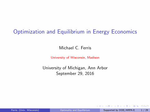
Power generation, transmission and distribution
Determine generators’ output to reliably meet the loadI∑
Gen MW ≥∑
Load MW, at all times.I Power flows cannot exceed lines’ transfer capacity.
Ferris (Univ. Wisconsin) Optimality and Equilibrium Supported by DOE/ARPA-E 2 / 29
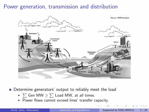
Single market, single good: equilibrium
Walras: 0 ≤ s(π)− d(π) ⊥ π ≥ 0
Market design and rules tofoster competitivebehavior/efficiency
Spatial extension: LocationalMarginal Prices (LMP) at nodes(buses) in the network
Supply arises often from a generatoroffer curve (lumpy)
Technologies and physics affectproduction and distribution
Ferris (Univ. Wisconsin) Optimality and Equilibrium Supported by DOE/ARPA-E 3 / 29
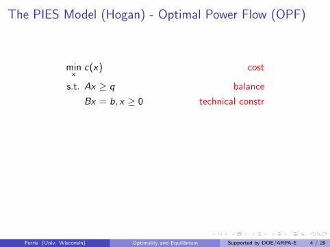
The PIES Model (Hogan) - Optimal Power Flow (OPF)
minx
c(x) cost
s.t. Ax ≥ q balance
Bx = b, x ≥ 0 technical constr
q = d(π): issue is that π is the multiplier on the “balance” constraint
Such multipliers (LMP’s) are critical to operation of market
Can try to solve the problem iteratively (shooting method):
πnew ∈ multiplier(OPF (d(π)))
Ferris (Univ. Wisconsin) Optimality and Equilibrium Supported by DOE/ARPA-E 4 / 29
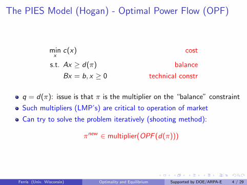
The PIES Model (Hogan) - Optimal Power Flow (OPF)
minx
c(x) cost
s.t. Ax ≥ d(π) balance
Bx = b, x ≥ 0 technical constr
q = d(π): issue is that π is the multiplier on the “balance” constraint
Such multipliers (LMP’s) are critical to operation of market
Can try to solve the problem iteratively (shooting method):
πnew ∈ multiplier(OPF (d(π)))
Ferris (Univ. Wisconsin) Optimality and Equilibrium Supported by DOE/ARPA-E 4 / 29
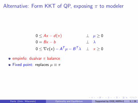
Alternative: Form KKT of QP, exposing π to modeler
0 ≤ Ax − d(π) ⊥ µ ≥ 0
0 = Bx − b ⊥ λ
0 ≤ ∇c(x)− ATµ− BTλ ⊥ x ≥ 0
empinfo: dualvar π balance
Fixed point: replaces µ ≡ π
Ferris (Univ. Wisconsin) Optimality and Equilibrium Supported by DOE/ARPA-E 5 / 29
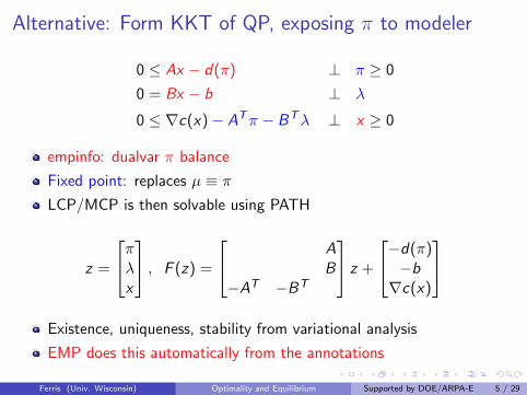
Alternative: Form KKT of QP, exposing π to modeler
0 ≤ Ax − d(π) ⊥ π ≥ 0
0 = Bx − b ⊥ λ
0 ≤ ∇c(x)− ATπ − BTλ ⊥ x ≥ 0
empinfo: dualvar π balance
Fixed point: replaces µ ≡ πLCP/MCP is then solvable using PATH
z =
πλx
, F (z) =
AB
−AT −BT
z +
−d(π)−b∇c(x)
Existence, uniqueness, stability from variational analysis
EMP does this automatically from the annotations
Ferris (Univ. Wisconsin) Optimality and Equilibrium Supported by DOE/ARPA-E 5 / 29
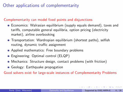
Other applications of complementarity
Complementarity can model fixed points and disjunctions
Economics: Walrasian equilibrium (supply equals demand), taxes andtariffs, computable general equilibria, option pricing (electricitymarket), airline overbooking
Transportation: Wardropian equilibrium (shortest paths), selfishrouting, dynamic traffic assignment
Applied mathematics: Free boundary problems
Engineering: Optimal control (ELQP)
Mechanics: Structure design, contact problems (with friction)
Geology: Earthquake propogation
Good solvers exist for large-scale instances of Complementarity Problems
Ferris (Univ. Wisconsin) Optimality and Equilibrium Supported by DOE/ARPA-E 6 / 29
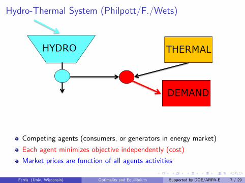
Hydro-Thermal System (Philpott/F./Wets)
Let us assume that 1 > 0 and p(!)2(!) > 0 for every ! 2 . This corresponds toa solution of SP meeting the demand constraints exactly, and being able to save moneyby reducing demand in each time period and in each state of the world. Under this as-sumption TP(i) and HP(i) also have unique solutions. Since they are convex optimizationproblems their solution will be determined by their Karush-Kuhn-Tucker (KKT) condi-tions. We dene the competitive equilibrium to be a solution to the following variationalproblem:
CE: (u1(i); u2(i; !)) 2 argmaxHP(i), i 2 H(v1(j); v2(j; !)) 2 argmaxTP(j), j 2 T0
Pi2H Ui (u1(i)) +
Pj2T v1(j) d1 ? 1 0;
0 +P
i2H Ui (u2(i; !)) +P
j2T v2(j; !) d2(!) ? 2(!) 0; ! 2 :
This gives the following result.
Proposition 2 Suppose every agent is risk neutral and has knowledge of all deterministicdata, as well as sharing the same probability distribution for inows. Then the solutionto SP is the same as the solution to CE.
3.1 Example
Throughout this paper we will illustrate the concepts using the hydro-thermal systemwith one reservoir and one thermal plant, as shown in Figure 1. We let thermal cost be
Figure 1: Example hydro-thermal system.
C (v) = v2, and dene
U(u) = 1:5u 0:015u2
V (x) = 30 3x+ 0:025x2
We assume inow 4 in period 1, and inows of 1; 2; : : : ; 10 with equal probability in eachscenario in period 2. With an initial storage level of 10 units this gives the competitiveequilibrium shown in Table 1. The central plan that maximizes expected welfare (byminimizing expected generation and future cost) is shown in Table 2. One can observethat the two solutions are identical, as predicted by Proposition 2.
6
Competing agents (consumers, or generators in energy market)
Each agent minimizes objective independently (cost)
Market prices are function of all agents activities
Ferris (Univ. Wisconsin) Optimality and Equilibrium Supported by DOE/ARPA-E 7 / 29
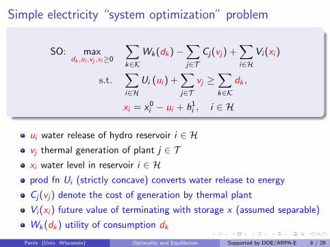
Simple electricity “system optimization” problem
SO: maxdk ,ui ,vj ,xi≥0
∑k∈K
Wk(dk)−∑j∈T
Cj(vj) +∑i∈H
Vi (xi )
s.t.∑i∈H
Ui (ui ) +∑j∈T
vj ≥∑k∈K
dk ,
xi = x0i − ui + h1i , i ∈ H
ui water release of hydro reservoir i ∈ Hvj thermal generation of plant j ∈ Txi water level in reservoir i ∈ Hprod fn Ui (strictly concave) converts water release to energy
Cj(vj) denote the cost of generation by thermal plant
Vi (xi ) future value of terminating with storage x (assumed separable)
Wk(dk) utility of consumption dk
Ferris (Univ. Wisconsin) Optimality and Equilibrium Supported by DOE/ARPA-E 8 / 29
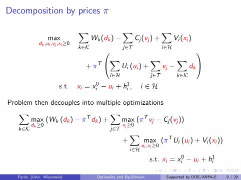
Decomposition by prices π
maxdk ,ui ,vj ,xi≥0
∑k∈K
Wk(dk)−∑j∈T
Cj(vj) +∑i∈H
Vi (xi )
+ πT
∑i∈H
Ui (ui ) +∑j∈T
vj −∑k∈K
dk
s.t. xi = x0i − ui + h1i , i ∈ H
Problem then decouples into multiple optimizations∑k∈K
maxdk≥0
(Wk (dk)− πTdk) +∑j∈T
maxvj≥0
(πT vj − Cj(vj))
+∑i∈H
maxui ,xi≥0
(πTUi (ui ) + Vi (xi ))
s.t. xi = x0i − ui + h1i
Ferris (Univ. Wisconsin) Optimality and Equilibrium Supported by DOE/ARPA-E 9 / 29
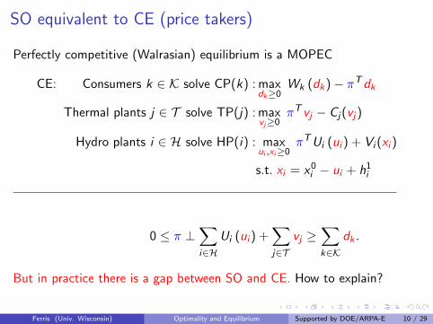
SO equivalent to CE (price takers)
Perfectly competitive (Walrasian) equilibrium is a MOPEC
CE: Consumers k ∈ K solve CP(k) : maxdk≥0
Wk (dk)− πTdk
Thermal plants j ∈ T solve TP(j) : maxvj≥0
πT vj − Cj(vj)
Hydro plants i ∈ H solve HP(i) : maxui ,xi≥0
πTUi (ui ) + Vi (xi )
s.t. xi = x0i − ui + h1i
0 ≤ π ⊥∑i∈H
Ui (ui ) +∑j∈T
vj ≥∑k∈K
dk .
But in practice there is a gap between SO and CE. How to explain?
Ferris (Univ. Wisconsin) Optimality and Equilibrium Supported by DOE/ARPA-E 10 / 29
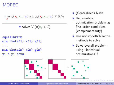
MOPEC
minxiθi (xi , x−i , π) s.t. gi (xi , x−i , π) ≤ 0,∀i
π solves VI(h(x , ·),C )
equilibrium
min theta(1) x(1) g(1)
...
min theta(m) x(m) g(m)
vi h pi cons
(Generalized) Nash
Reformulateoptimization problem asfirst order conditions(complementarity)
Use nonsmooth Newtonmethods to solve
Solve overall problemusing “individualoptimizations”?
Trade/Policy Model (MCP)
• Split model (18,000 vars) via region
• Gauss-Seidel, Jacobi, Asynchronous • 87 regional subprobs, 592 solves
= +
Ferris (Univ. Wisconsin) Optimality and Equilibrium Supported by DOE/ARPA-E 11 / 29
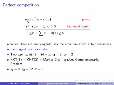
Perfect competition
maxxi
πT xi − ci (xi ) profit
s.t. Bixi = bi , xi ≥ 0 technical constr
0 ≤π ⊥∑i
xi − d(π) ≥ 0
When there are many agents, assume none can affect π by themselves
Each agent is a price taker
Two agents, d(π) = 24− π, c1 = 3, c2 = 2
KKT(1) + KKT(2) + Market Clearing gives ComplementarityProblem
x1 = 0, x2 = 22, π = 2
Ferris (Univ. Wisconsin) Optimality and Equilibrium Supported by DOE/ARPA-E 12 / 29
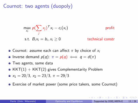
Cournot: two agents (duopoly)
maxxi
p(∑j
xj)T xi − ci (xi ) profit
s.t. Bixi = bi , xi ≥ 0 technical constr
Cournot: assume each can affect π by choice of xi
Inverse demand p(q): π = p(q) ⇐⇒ q = d(π)
Two agents, same data
KKT(1) + KKT(2) gives Complementarity Problem
x1 = 20/3, x2 = 23/3, π = 29/3
Exercise of market power (some price takers, some Cournot)
Ferris (Univ. Wisconsin) Optimality and Equilibrium Supported by DOE/ARPA-E 13 / 29
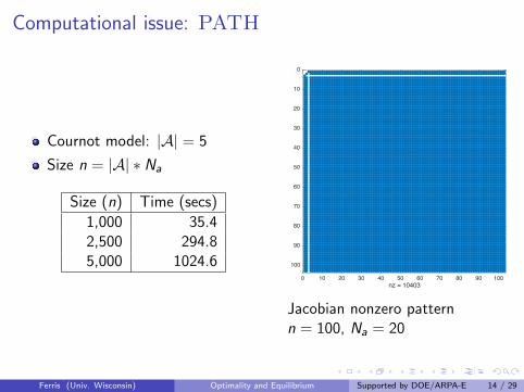
Computational issue: PATH
Cournot model: |A| = 5
Size n = |A| ∗ Na
Size (n) Time (secs)
1,000 35.42,500 294.85,000 1024.6
0 10 20 30 40 50 60 70 80 90 100nz = 10403
0
10
20
30
40
50
60
70
80
90
100
Jacobian nonzero patternn = 100, Na = 20
Ferris (Univ. Wisconsin) Optimality and Equilibrium Supported by DOE/ARPA-E 14 / 29
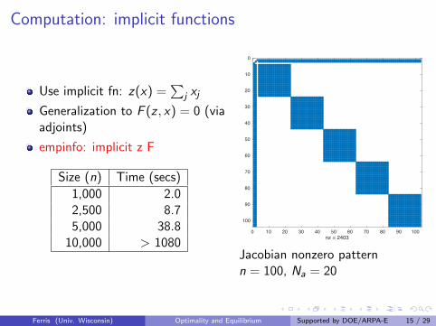
Computation: implicit functions
Use implicit fn: z(x) =∑
j xj
Generalization to F (z , x) = 0 (viaadjoints)
empinfo: implicit z F
Size (n) Time (secs)
1,000 2.02,500 8.75,000 38.8
10,000 > 10800 10 20 30 40 50 60 70 80 90 100
nz = 2403
0
10
20
30
40
50
60
70
80
90
100
Jacobian nonzero patternn = 100, Na = 20
Ferris (Univ. Wisconsin) Optimality and Equilibrium Supported by DOE/ARPA-E 15 / 29
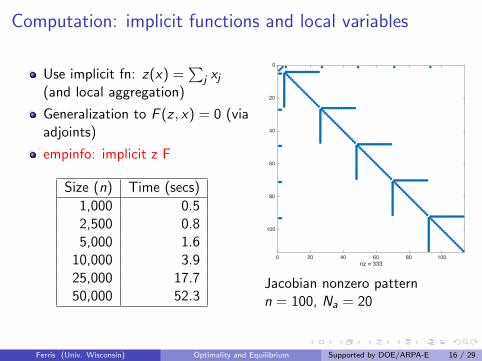
Computation: implicit functions and local variables
Use implicit fn: z(x) =∑
j xj(and local aggregation)
Generalization to F (z , x) = 0 (viaadjoints)
empinfo: implicit z F
Size (n) Time (secs)
1,000 0.52,500 0.85,000 1.6
10,000 3.925,000 17.750,000 52.3
0 20 40 60 80 100nz = 333
0
20
40
60
80
100
Jacobian nonzero patternn = 100, Na = 20
Ferris (Univ. Wisconsin) Optimality and Equilibrium Supported by DOE/ARPA-E 16 / 29
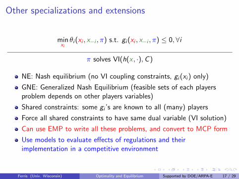
Other specializations and extensions
minxiθi (xi , x−i , π) s.t. gi (xi , x−i , π) ≤ 0, ∀i
π solves VI(h(x , ·),C )
NE: Nash equilibrium (no VI coupling constraints, gi (xi ) only)
GNE: Generalized Nash Equilibrium (feasible sets of each playersproblem depends on other players variables)
Shared constraints: some gi ’s are known to all (many) players
Force all shared constraints to have same dual variable (VI solution)
Can use EMP to write all these problems, and convert to MCP form
Use models to evaluate effects of regulations and theirimplementation in a competitive environment
Ferris (Univ. Wisconsin) Optimality and Equilibrium Supported by DOE/ARPA-E 17 / 29
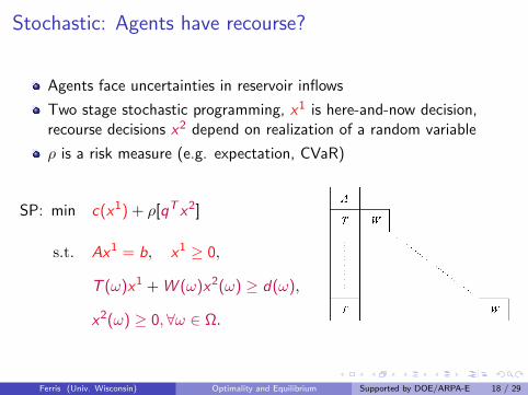
Stochastic: Agents have recourse?
Agents face uncertainties in reservoir inflows
Two stage stochastic programming, x1 is here-and-now decision,recourse decisions x2 depend on realization of a random variable
ρ is a risk measure (e.g. expectation, CVaR)
SP: min c(x1) + ρ[qT x2]
s.t. Ax1 = b, x1 ≥ 0,
T (ω)x1 + W (ω)x2(ω) ≥ d(ω),
x2(ω) ≥ 0,∀ω ∈ Ω.
A
T W
T
igure Constraints matrix structure of 15)
problem by suitable subgradient methods in an outer loop. In the inner loop, the second-stage problem is solved for various r i g h t h a n d sides. Convexity of the master is inherited from the convexity of the value function in linear programming. In dual decomposition, (Mulvey and Ruszczyhski 1995, Rockafellar and Wets 1991), a convex non-smooth function of Lagrange multipliers is minimized in an outer loop. Here, convexity is granted by fairly general reasons that would also apply with integer variables in 15). In the inner loop, subproblems differing only in their r i g h t h a n d sides are to be solved. Linear (or convex) programming duality is the driving force behind this procedure that is mainly applied in the multi-stage setting.
When following the idea of primal decomposition in the presence of integer variables one faces discontinuity of the master in the outer loop. This is caused by the fact that the value function of an MILP is merely lower semicontinuous in general Computations have to overcome the difficulty of lower semicontinuous minimization for which no efficient methods exist up to now. In Car0e and Tind (1998) this is analyzed in more detail. In the inner loop, MILPs arise which differ in their r i g h t h a n d sides only. Application of Gröbner bases methods from computational algebra has led to first computational techniques that exploit this similarity in case of pure-integer second-stage problems, see Schultz, Stougie, and Van der Vlerk (1998).
With integer variables, dual decomposition runs into trouble due to duality gaps that typically arise in integer optimization. In L0kketangen and Woodruff (1996) and Takriti, Birge, and Long (1994, 1996), Lagrange multipliers are iterated along the lines of the progressive hedging algorithm in Rockafellar and Wets (1991) whose convergence proof needs continuous variables in the original problem. Despite this lack of theoretical underpinning the computational results in L0kketangen and Woodruff (1996) and Takriti, Birge, and Long (1994 1996), indicate that for practical problems acceptable solutions can be found this way. A branch-and-bound method for stochastic integer programs that utilizes stochastic bounding procedures was derived in Ruszczyriski, Ermoliev, and Norkin (1994). In Car0e and Schultz (1997) a dual decomposition method was developed that combines Lagrangian relaxation of non-anticipativity constraints with branch-and-bound. We will apply this method to the model from Section and describe the main features in the remainder of the present section.
The idea of scenario decomposition is well known from stochastic programming with continuous variables where it is mainly used in the mul t i s tage case. For stochastic integer programs scenario decomposition is advantageous already in the two-stage case. The idea is
Ferris (Univ. Wisconsin) Optimality and Equilibrium Supported by DOE/ARPA-E 18 / 29
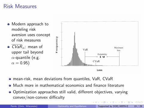
Risk Measures
Modern approach tomodeling riskaversion uses conceptof risk measures
CVaRα: mean ofupper tail beyondα-quantile (e.g.α = 0.95)
VaR, CVaR, CVaR+ and CVaR-
Loss
Fre
qu
en
cy
1111 −−−−αααα
VaR
CVaR
Probability
Maximumloss
mean-risk, mean deviations from quantiles, VaR, CVaR
Much more in mathematical economics and finance literature
Optimization approaches still valid, different objectives, varyingconvex/non-convex difficulty
Ferris (Univ. Wisconsin) Optimality and Equilibrium Supported by DOE/ARPA-E 19 / 29
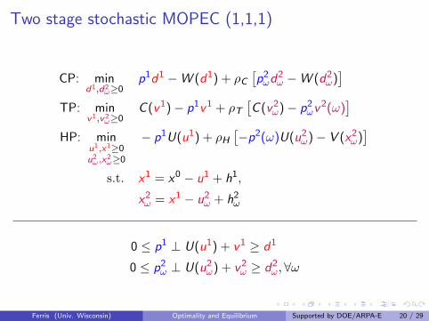
Two stage stochastic MOPEC (1,1,1)
CP: mind1
,d2ω
≥0p1d1 −W (d1)
+ ρC[p2ωd
2ω −W (d2
ω)]
TP: minv1
,v2ω
≥0C (v1)− p1v1
+ ρT[C (v2ω)− p2ωv
2(ω)]
HP: minu1,x1≥0
u2ω ,x2ω≥0
− p1U(u1)
+ ρH[−p2(ω)U(u2ω)− V (x2ω)
]
s.t. x1 = x0 − u1 + h1,
x2ω = x1 − u2ω + h2ω
0 ≤ p1 ⊥ U(u1) + v1 ≥ d1
0 ≤ p2ω ⊥ U(u2ω) + v2ω ≥ d2ω,∀ω
Ferris (Univ. Wisconsin) Optimality and Equilibrium Supported by DOE/ARPA-E 20 / 29
Two stage stochastic MOPEC (1,1,1)
CP: mind1,d2
ω≥0p1d1 −W (d1) + ρC
[p2ωd
2ω −W (d2
ω)]
TP: minv1,v2
ω≥0C (v1)− p1v1 + ρT
[C (v2ω)− p2ωv
2(ω)]
HP: minu1,x1≥0u2ω ,x
2ω≥0
− p1U(u1) + ρH[−p2(ω)U(u2ω)− V (x2ω)
]s.t. x1 = x0 − u1 + h1,
x2ω = x1 − u2ω + h2ω
0 ≤ p1 ⊥ U(u1) + v1 ≥ d1
0 ≤ p2ω ⊥ U(u2ω) + v2ω ≥ d2ω,∀ω
Ferris (Univ. Wisconsin) Optimality and Equilibrium Supported by DOE/ARPA-E 20 / 29
0
1
2
3
44
5
6
7
8
9
10
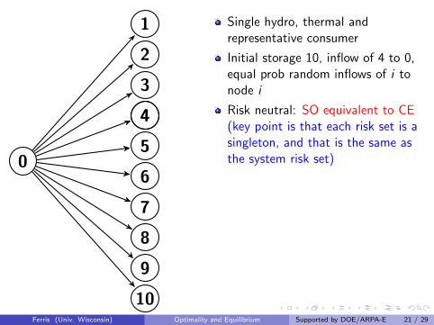
Single hydro, thermal andrepresentative consumer
Initial storage 10, inflow of 4 to 0,equal prob random inflows of i tonode i
Risk neutral: SO equivalent to CE(key point is that each risk set is asingleton, and that is the same asthe system risk set)
Each agent has its own riskmeasure, e.g. 0.8EV + 0.2CVaR
Is there a system risk measure?
Is there a system optimizationproblem?
min∑i
C (x1i ) + ρi(C (x2i (ω))
)????
Ferris (Univ. Wisconsin) Optimality and Equilibrium Supported by DOE/ARPA-E 21 / 29
0
1
2
3
44
5
6
7
8
9
10
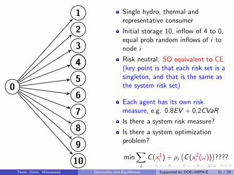
Single hydro, thermal andrepresentative consumer
Initial storage 10, inflow of 4 to 0,equal prob random inflows of i tonode i
Risk neutral: SO equivalent to CE(key point is that each risk set is asingleton, and that is the same asthe system risk set)
Each agent has its own riskmeasure, e.g. 0.8EV + 0.2CVaR
Is there a system risk measure?
Is there a system optimizationproblem?
min∑i
C (x1i ) + ρi(C (x2i (ω))
)????
Ferris (Univ. Wisconsin) Optimality and Equilibrium Supported by DOE/ARPA-E 21 / 29
Equilibrium or optimization?
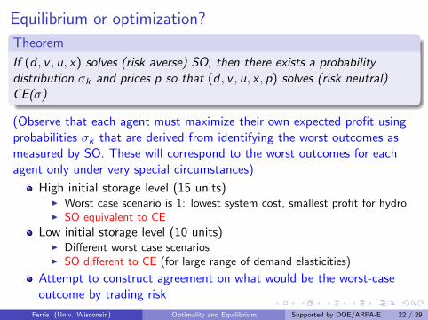
Theorem
If (d , v , u, x) solves (risk averse) SO, then there exists a probabilitydistribution σk and prices p so that (d , v , u, x , p) solves (risk neutral)CE(σ)
(Observe that each agent must maximize their own expected profit usingprobabilities σk that are derived from identifying the worst outcomes asmeasured by SO. These will correspond to the worst outcomes for eachagent only under very special circumstances)
High initial storage level (15 units)I Worst case scenario is 1: lowest system cost, smallest profit for hydroI SO equivalent to CE
Low initial storage level (10 units)I Different worst case scenariosI SO different to CE (for large range of demand elasticities)
Attempt to construct agreement on what would be the worst-caseoutcome by trading risk
Ferris (Univ. Wisconsin) Optimality and Equilibrium Supported by DOE/ARPA-E 22 / 29

Contracts in MOPEC (Philpott/F./Wets)
Can we modify (complete) system to have a social optimum bytrading risk?
How do we design these instruments? How many are needed? Whatis cost of deficiency?
Facilitated by allowing contracts bought now, for goods deliveredlater (e.g. Arrow-Debreu Securities)
Conceptually allows to transfer goods from one period to another(provides wealth retention or pricing of ancilliary services in energymarket)
Can investigate new instruments to mitigate risk, or move to systemoptimal solutions from equilibrium (or market) solutions
Ferris (Univ. Wisconsin) Optimality and Equilibrium Supported by DOE/ARPA-E 23 / 29
Theory and Observations
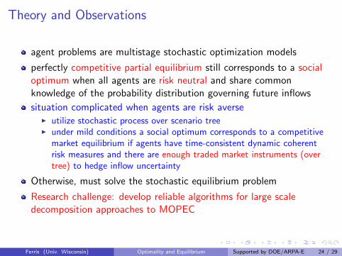
agent problems are multistage stochastic optimization models
perfectly competitive partial equilibrium still corresponds to a socialoptimum when all agents are risk neutral and share commonknowledge of the probability distribution governing future inflows
situation complicated when agents are risk averseI utilize stochastic process over scenario treeI under mild conditions a social optimum corresponds to a competitive
market equilibrium if agents have time-consistent dynamic coherentrisk measures and there are enough traded market instruments (overtree) to hedge inflow uncertainty
Otherwise, must solve the stochastic equilibrium problem
Research challenge: develop reliable algorithms for large scaledecomposition approaches to MOPEC
Ferris (Univ. Wisconsin) Optimality and Equilibrium Supported by DOE/ARPA-E 24 / 29
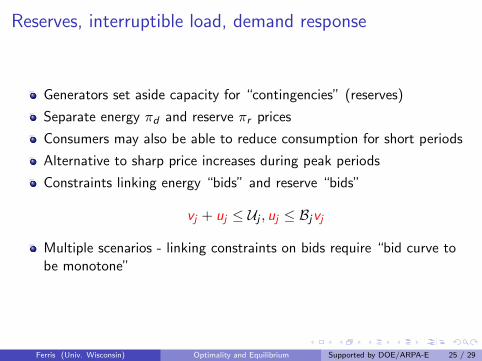
Reserves, interruptible load, demand response
Generators set aside capacity for “contingencies” (reserves)
Separate energy πd and reserve πr prices
Consumers may also be able to reduce consumption for short periods
Alternative to sharp price increases during peak periods
Constraints linking energy “bids” and reserve “bids”
vj + uj ≤ Uj , uj ≤ Bjvj
Multiple scenarios - linking constraints on bids require “bid curve tobe monotone”
Ferris (Univ. Wisconsin) Optimality and Equilibrium Supported by DOE/ARPA-E 25 / 29

Price taking: model is MOPEC
Consumption dk , demand response rk , energy vj , reserves uj , prices π
Consumer max(dk ,rk )∈C
utility(dk)− πdTdk + profit(rk , πr )
Generator max(vj ,uj )∈G
profit(vj , πd) + profit(uj , πr )
s.t. vj + uj ≤ Uj , uj ≤ BjvjTransmission max
f ∈Fcongestion rates(f , πd)
Market clearing
0 ≤ πd ⊥∑j
vj −∑k
dk −Af ≥ 0
0 ≤ πr ⊥∑j
uj +∑k
rk −R ≥ 0
Ferris (Univ. Wisconsin) Optimality and Equilibrium Supported by DOE/ARPA-E 26 / 29
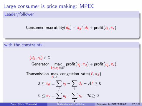
Large consumer is price making: MPEC
Leader/follower
Consumer max utility(dk)− πdTdk + profit(rk , πr )
with the constraints:
(dk , rk) ∈ CGenerator max
(vj ,uj )∈G′profit(vj , πd) + profit(uj , πr )
Transmission maxf ∈F
congestion rates(f , πd)
0 ≤ πd ⊥∑j
vj −∑k
dk −Af ≥ 0
0 ≤ πr ⊥∑j
uj +∑k
rk −R ≥ 0
Ferris (Univ. Wisconsin) Optimality and Equilibrium Supported by DOE/ARPA-E 27 / 29
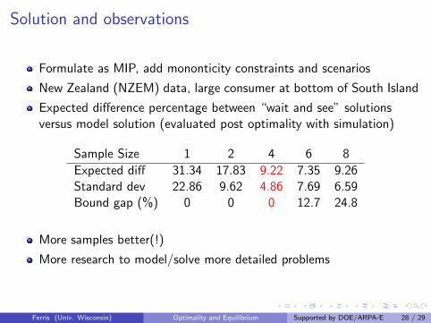
Solution and observations
Formulate as MIP, add mononticity constraints and scenarios
New Zealand (NZEM) data, large consumer at bottom of South Island
Expected difference percentage between “wait and see” solutionsversus model solution (evaluated post optimality with simulation)
Sample Size 1 2 4 6 8
Expected diff 31.34 17.83 9.22 7.35 9.26Standard dev 22.86 9.62 4.86 7.69 6.59Bound gap (%) 0 0 0 12.7 24.8
More samples better(!)
More research to model/solve more detailed problems
Ferris (Univ. Wisconsin) Optimality and Equilibrium Supported by DOE/ARPA-E 28 / 29
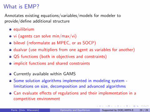
What is EMP?
Annotates existing equations/variables/models for modeler toprovide/define additional structure
equilibrium
vi (agents can solve min/max/vi)
bilevel (reformulate as MPEC, or as SOCP)
dualvar (use multipliers from one agent as variables for another)
QS functions (both in objectives and constraints)
implicit functions and shared constraints
Currently available within GAMS
Some solution algorithms implemented in modeling system -limitations on size, decomposition and advanced algorithms
Can evaluate effects of regulations and their implementation in acompetitive environment
Ferris (Univ. Wisconsin) Optimality and Equilibrium Supported by DOE/ARPA-E 29 / 29
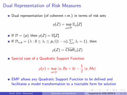
Dual Representation of Risk Measures
Dual representation (of coherent r.m.) in terms of risk sets
ρ(Z ) = supµ∈D
Eµ[Z ]
If D = p then ρ(Z ) = E[Z ]
If Dα,p = λ : 0 ≤ λi ≤ pi/(1− α),∑
i λi = 1, then
ρ(Z ) = CVaRα(Z )
Special case of a Quadratic Support Function
ρ(y) = supu∈U〈u,By + b〉 − 1
2〈u,Mu〉
EMP allows any Quadratic Support Function to be defined andfacilitates a model transformation to a tractable form for solution
Ferris (Univ. Wisconsin) Optimality and Equilibrium Supported by DOE/ARPA-E 1 / 3
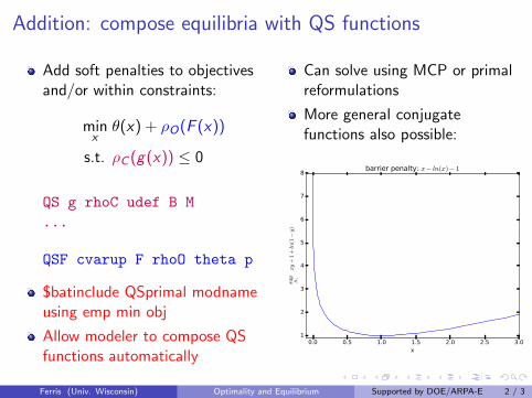
Addition: compose equilibria with QS functions
Add soft penalties to objectivesand/or within constraints:
minxθ(x) + ρO(F (x))
s.t. ρC (g(x)) ≤ 0
QS g rhoC udef B M
...
QSF cvarup F rhoO theta p
$batinclude QSprimal modnameusing emp min obj
Allow modeler to compose QSfunctions automatically
Can solve using MCP or primalreformulations
More general conjugatefunctions also possible:
0.0 0.5 1.0 1.5 2.0 2.5 3.0x
1
2
3
4
5
6
7
8
sup
R+
xy+
1+ln
(1−y)
barrier penalty: x− ln(x)− 1
Ferris (Univ. Wisconsin) Optimality and Equilibrium Supported by DOE/ARPA-E 2 / 3
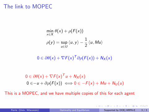
The link to MOPEC
minx∈X
θ(x) + ρ(F (x))
ρ(y) = supu∈U〈u, y〉 − 1
2〈u,Mu〉
0 ∈ ∂θ(x) +∇F (x)T∂ρ(F (x)) + NX (x)
0 ∈ ∂θ(x) +∇F (x)Tu + NX (x)
0 ∈−u + ∂ρ(F (x)) ⇐⇒ 0 ∈ −F (x) + Mu + NU(u)
This is a MOPEC, and we have multiple copies of this for each agent
Ferris (Univ. Wisconsin) Optimality and Equilibrium Supported by DOE/ARPA-E 3 / 3