Embed Size (px)
Citation preview
ISSN 0280-5316 ISRN LUTFD2/TFRT--5697--SE
Optimal Vehicle Dynamics – Yaw Rate and Side Slip Angle Control Using
4-Wheel Steering
Nenad Lazic
Department of Automatic Control Lund Institute of Technology
October 2002

Document name MASTER THESIS Date of issue October 2002
Department of Automatic Control Lund Institute of Technology Box 118 SE-221 00 Lund Sweden Document Number
ISRN LUTFD2/TFRT--5697--SE Supervisor Anders Rantzer, LTH Jens Kalkkuhl DaimlerChrysler AG, Stuttgart
Author(s)
Nenad Lasic
Sponsoring organization
Title and subtitle Optimal Vehicle Dynamics – Yaw Rate and Side Slip Angle Control Using 4-Wheel Steering. (Optimal fordonsdynamik vid 4-hjulsstyrning).
Abstract
The development of steer-by-wire involves an increased amount of possibilities for control in future cars. For example, the experimental vehicle available has both front and rear wheel steering. This enables a simultaneous multivariable control of both the yaw rate and the side slip angle. The today existing control approach is designed in the time domain and it has a decoupled control structure, where the yaw rate is controlled by the front wheel steering angle, and the side slip angle is controlled by the rear wheel steering angle. With this approach there are some major difficulties, such as constraint handling and lack of robustness to plant uncertainties, to time delays and to actuator or sensor failure. To solve these problems, a multivariable control scheduling system can be used that has already been applied to robotics, satellite attitude control and ship control but is a novelty for the field of automotive control. It is a coupling control approach, based on Individual Channel Design in the frequency domain, ICD, and considers the internal cross-coupling of the plant. It has been shown that meeting the requirements is not trivial, and a tradeoff has to be done between high performance and entirely meeting the specifications. However, the design shows a considerable degree of both robustness and integrity, which has been verified in theory as well as in simulations, but has to be further checked in real experiments.
Keywords
Classification system and/or index terms (if any)
Supplementary bibliographical information ISSN and key title 0280-5316
ISBN
Language English
Number of pages 90
Security classification
Recipient’s notes
The report may be ordered from the Department of Automatic Control or borrowed through: University Library 2, Box 3, SE-221 00 Lund, Sweden Fax +46 46 222 44 22 E-mail [email protected]

Optimal Vehicle Dynamics - Yaw Rate and
Side Slip Angle Control Using 4-Wheel
Steering
Nenad Lazic
October 23, 2002


Contents
1 Introduction 21.1 Problem Formulation . . . . . . . . . . . . . . . . . . . . . . . 21.2 Thesis Outline . . . . . . . . . . . . . . . . . . . . . . . . . . . 3
2 The Car Model 42.1 Wheel Model . . . . . . . . . . . . . . . . . . . . . . . . . . . 52.2 The One-track Bicycle Model . . . . . . . . . . . . . . . . . . 82.3 Model Parameters . . . . . . . . . . . . . . . . . . . . . . . . . 12
3 Control Strategies and Specifications 143.1 Specifications . . . . . . . . . . . . . . . . . . . . . . . . . . . 143.2 The Feedforward . . . . . . . . . . . . . . . . . . . . . . . . . 15
3.2.1 Linear system . . . . . . . . . . . . . . . . . . . . . . . 163.2.2 Nonlinear system . . . . . . . . . . . . . . . . . . . . . 173.2.3 Combining the nonlinear feedforward and the linear
feedback . . . . . . . . . . . . . . . . . . . . . . . . . . 183.3 The Feedback . . . . . . . . . . . . . . . . . . . . . . . . . . . 19
4 Feedback - Individual Channel Design 214.1 Theory . . . . . . . . . . . . . . . . . . . . . . . . . . . . . . . 214.2 Adding Actuators . . . . . . . . . . . . . . . . . . . . . . . . . 244.3 The Main Advantages and Disadvantages . . . . . . . . . . . . 254.4 The Design Procedure . . . . . . . . . . . . . . . . . . . . . . 27
5 Feedback Design - Results 285.1 Controller Scheduling . . . . . . . . . . . . . . . . . . . . . . . 395.2 System Integrity and Robustness . . . . . . . . . . . . . . . . 41
6 Simulation Results 566.1 Introducing Time Delay . . . . . . . . . . . . . . . . . . . . . 566.2 Keeping the Time Delay and Breaking the Second Loop . . . . 72
7 Conclusions and Future Work 76
A Matlab Commands 77A.1 State Space Modelling . . . . . . . . . . . . . . . . . . . . . . 77A.2 An Iteration Step . . . . . . . . . . . . . . . . . . . . . . . . . 78A.3 Making a PID-controller . . . . . . . . . . . . . . . . . . . . . 78
A.3.1 Converting into PID-parameters . . . . . . . . . . . . . 78A.3.2 Scheduling with respect to speed . . . . . . . . . . . . 79A.3.3 Discretising the controller . . . . . . . . . . . . . . . . 80
i

Acknowledgements
This thesis was done in cooperation between DaimlerChrysler AG, Stuttgart,and the Department of Automatic Control, Lund Institute of Technology. Ithas been carried out at the Department of Driver Assistant Systems, Daim-lerChrysler, in Esslingen, just outside Stuttgart, from March to September2002.
I am grateful to all the people at the department in Esslingen. Especially Iwould like to thank Dr. Jens Kalkkuhl for his great supervising and supportthroughout my work. I also would like to thank Prof. Anders Rantzerfor giving me the opportunity to do this thesis and for giving me valuablecomments on the report.
Lund, October 2002Nenad Lazic
ii
1 INTRODUCTION 2
1 Introduction
1.1 Problem Formulation
Today’s cars are becoming more and more sophisticated. They contain moreelectrical hardware components and less mechanical and hydraulic ones. Ex-amples of this are the actuators used for control such as in brake-by-wire,steer-by-wire and active suspension. In future cars there might be a verylarge number of possible configurations for these actuators. This means thatforces and torque for control action can be applied in many different ways.What we want is to optimally employ these actuators such that
• control is achieved with minimum control action
• the solution is robust to plant uncertainties, and a failure of one actu-ator can be compensated by the remaining ones
• the controller can be adapted to any specific actuator configuration
To achieve all three objectives, a multivariable control scheduling systemhas to be used that has already been applied to robotics, satellite attitudecontrol and ship control but is a novelty for the field of automotive control.It requires the solution of problems unique to automotive control such as
• handling uncertain nonlinear tyre forces
• time varying constraints on the maximum available tyre forces due tochanging road conditions
Using existing modelled vehicle dynamics, reference yaw rate and side slipangle are generated from a driver command. With proper model matching,and considering disturbances and uncertainties, control commands should begiven such that the reference is followed.
In this work 4 wheel steering (front and rear axle) is used for control,with yaw rate and side slip angle as outputs from the car, and front andrear wheel steering angles as the input to the car. The problem is to controlthe yaw rate and side slip angle simultaneously (normally, the side slip anglehas to be kept under a certain threshold), and at the same time fulfil thespecifications that are set up for the control system.
The internal structure of the system involves a certain degree of cross-coupling between inputs and outputs. An approach with a decoupled con-troller structure, as well as a model based state space design in the timedomain, where one controller is used for yaw rate and another for side slipangle, constructed independently of each other, already exists. The front

1 INTRODUCTION 3
wheel steering angle is generated using both feedforward and feedback, andfor the rear wheel steering angle only feedforward is used. This decouplingapproach has some major disadvantages. One is the lack of robustness, bothto plant uncertainties and time delays. The limitations in constraint handlingare another disadvantage.
By also taking the dependency between yaw rate and side slip angle con-trol into account, and using a coupling approach, a more robust solution canbe obtained that meets the theory and specifications in a better way. Theintention is to use feedforward and feedback for both rear and front wheelsteering. However, feedback design will be the central point.
1.2 Thesis Outline
This work consists of three main parts. The first part, system modelling,problem specification and survey of different design strategies, is discussedin chapter 2 to chapter 4. In chapter 2 the fundamental concepts of ve-hicle dynamics are explained. The general ideas and specifications of themultivariable controller design are discussed in chapter 3. Some ideas aboutfeedforward will be presented, but focus will be put on feedback design. Thefeedback design approach chosen for this work, Individual Channel Design,is explained in chapter 4. Beyond that, a rough structure for the controllerwill be discussed in the chapter.
The second part is the controller design. This will be described in chapter5. The software environment used for the design is Matlab, and in particularthe SISO root-locus design tool in Matlab.
Simulations and experimental results are the third part of this work.The simulations will be carried out in Matlab Simulink. A complete carmodel, containing the same dynamics as a real car, will be used to verifythe performance and robustness of the controller. The simulation results arediscussed in chapter 6. The most important parts of the Matlab code usedduring the design are given in the Appendix.
2 THE CAR MODEL 4
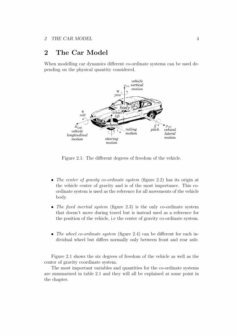
2 The Car Model
When modelling car dynamics different co-ordinate systems can be used de-pending on the physical quantity considered.
Figure 2.1: The different degrees of freedom of the vehicle.
• The center of gravity co-ordinate system (figure 2.2) has its origin atthe vehicle center of gravity and is of the most importance. This co-ordinate system is used as the reference for all movements of the vehiclebody.
• The fixed inertial system (figure 2.3) is the only co-ordinate systemthat doesn’t move during travel but is instead used as a reference forthe position of the vehicle, i.e the center of gravity co-ordinate system.
• The wheel co-ordinate system (figure 2.4) can be different for each in-dividual wheel but differs normally only between front and rear axle.
Figure 2.1 shows the six degrees of freedom of the vehicle as well as thecenter of gravity coordinate system.
The most important variables and quantities for the co-ordinate systemsare summarized in table 2.1 and they will all be explained at some point inthe chapter.

2 THE CAR MODEL 5
Figure 2.2: The CoG co-ordinate system and its main quantities.
Figure 2.3: The CoG co-ordinate system in relation to the inertial.
2.1 Wheel Model
The location of the wheel ground contact point (marked by P in figure 2.4)normally differs from the origin of the wheel co-ordinate system. Its exactlocation depends on the steering mechanism, the vertical normal force dis-tribution of the vehicle, the tyre stiffness and is described by the casters nu
and ns. The frictional forces (S and U in figure 2.4) that act on the wheelin the contact point determine the behaviour of the vehicle. The dynamiccharacteristics of these forces are nonlinear with respect to the wheel slip (see

2 THE CAR MODEL 6
W x
W y
W z L n
S n
S
U P
Figure 2.4: The wheel co-ordinate system. Road surface contact area viewedfrom above.
Table 2.1: Co-ordinate system variablesxCoG, yCoG, zCoG Axis for the center of gravity co-ordinate systemxW , yW , zW Axis for the wheel co-ordinate systemxIn, yIn, zIn Axis for the inertial co-ordinate systemψ Yaw angle (rotation about zCoG)α Tyre side slip angle (angle between xW and vW , the
wheel ground contact point velocity)δ Wheel steering angleβ Vehicle body side slip angle (angle between xCoG and
vCoG, the vehicle velocity)Sf/r Lateral wheel ground contact force (acting in the direc-
tion of yW )Uf/r Longitudinal wheel ground contact force (acting in the
direction of xW )vx The forward velocity, in the direction of xCoG
vy The lateral velocity, in the direction of yCoG
v The resulting velocity. Geometrical sum of vx and vy
Cs, Cu Tyre stiffness in the direction of yW and xW
λs, λu Wheel slip in the direction of yW and xW
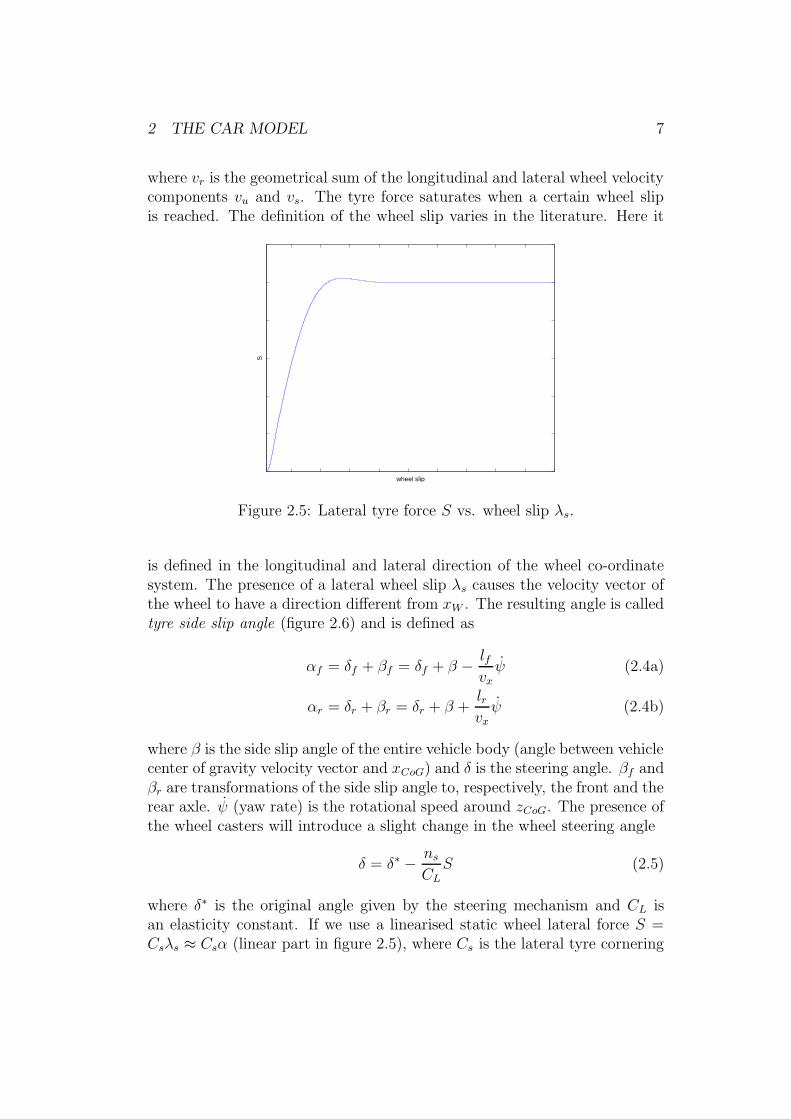
figure 2.5), which is defined as
λu =ωwheel · rwheel − vu
vr(2.1)
λs = sinα ≈ α (2.2)
λr =√
λ2u + λ2
s (2.3)
2 THE CAR MODEL 7
where vr is the geometrical sum of the longitudinal and lateral wheel velocitycomponents vu and vs. The tyre force saturates when a certain wheel slipis reached. The definition of the wheel slip varies in the literature. Here it
wheel slip
S
Figure 2.5: Lateral tyre force S vs. wheel slip λs.
is defined in the longitudinal and lateral direction of the wheel co-ordinatesystem. The presence of a lateral wheel slip λs causes the velocity vector ofthe wheel to have a direction different from xW . The resulting angle is calledtyre side slip angle (figure 2.6) and is defined as
αf = δf + βf = δf + β −lfvxψ (2.4a)
αr = δr + βr = δr + β +lrvxψ (2.4b)
where β is the side slip angle of the entire vehicle body (angle between vehiclecenter of gravity velocity vector and xCoG) and δ is the steering angle. βf andβr are transformations of the side slip angle to, respectively, the front and therear axle. ψ (yaw rate) is the rotational speed around zCoG. The presence ofthe wheel casters will introduce a slight change in the wheel steering angle
δ = δ∗ −ns
CLS (2.5)
where δ∗ is the original angle given by the steering mechanism and CL isan elasticity constant. If we use a linearised static wheel lateral force S =Csλs ≈ Csα (linear part in figure 2.5), where Cs is the lateral tyre cornering

2 THE CAR MODEL 8
stiffness, and combine it with equation (2.5), the resulting equation for thetyre force S will be
S =Cs
1 + Cs
CLns
(δ∗ + β) = C∗
sα∗ (2.6)
The virtual tyre stiffness C∗
s is reduced in comparison to Cs.The dynamic tyre characteristics can be modelled linearly or nonlinearly.
The linear approach simplifies the design but is of limited use:
S =∂S
∂λs
∣
∣
∣
∣
λs=λu=0
· λs = Csλs ≈ Csα (2.7)
U =∂U
∂λu
∣
∣
∣
∣
λs=λu=0
· λu = Cuλu (2.8)
The complete nonlinear model is [Niethammer]
S =
{
Csλs
(ξs−1)2+C∗
s ξsξs ≤ 1,
λs
λrµsFz ξs > 1
(2.9)
U =
{
Cuλu
(ξu−1)2+C∗
uξuξu ≤ 1,
λu
λrµuFz ξu > 1
(2.10)
with the following definitions of the normalised wheel slip
ξs =λr
λSmax(2.11)
ξu =λr
λUmax(2.12)
2.2 The One-track Bicycle Model
As a base for the controller design a linear one-track bicycle model is used(figure 2.6). This simple model considers front and rear wheel steering aswell as actuator dynamics. It is not very well purposed for simulation, butfor controller design it should be sufficient.
To obtain information about the behaviour of the system, in other wordsthe transfer function G(s), a state space representation is made, with theyaw rate, ψ, and the side slip angle at the rear axle, βr, as outputs and frontand rear wheel steering angles, (δf , δr), as inputs to the process. The input,output and state vectors are
u =
(
u1
u2
)
=
(
δfδr
)
(2.13)

2 THE CAR MODEL 9
f v f δ
f β f α
W x
W y
f S
f U
CoG x
CoG y
r δ
r β r α r U
r S
W y
W x
r v
f l
r l
v β
t ∂ ∂ ψ
Figure 2.6: The one-track bicycle model.

2 THE CAR MODEL 10
y =
(
y1
y2
)
=
(
ψβr
)
(2.14)
x =
ψβr
Sf
Sr
(2.15)
The force equations of the vehicle are
max = FXf + FXr = m(
vx − vyψ)
(2.16)
may = FY f + FY r = m(
vy + vxψ)
where FXf and FXr act in the vehicle direction and FY f and FY r are lateralforces. The moment equilibrium around the center of mass leads to thedifferential equation
Izzψ = FY f lf − FY rlr (2.17)
where the forces can be rewritten as
FXf = Uf cos δf − Sf sin δf (2.18)
FXr = Ur cos δr − Sr sin δr
FY f = Uf sin δf + Sf cos δf
FY r = Ur sin δr + Sr cos δr
By assuming small front and rear wheel steering angles, a linearisation canbe made:
cos δf = cos δr = 1 (2.19)
sin δf = δf
sin δr = δr
Uf = Ur = 0
Combining equation (2.18) with the equations (2.17) and (2.16) gives
ψ =1
Izz(lfSf − lrSr) (2.20)
vy = −vxψ +Sf + Sr
m(2.21)
The side slip angle β is defined as
β = arctan
(
−vy
vx
)
≈ −vy
vx(2.22)
2 THE CAR MODEL 11
Assuming a constant vx, and combining (2.21) with (2.22), gives the differ-ential equation for the side slip angle
β = ψ −Sf + Sr
mvx(2.23)
With
βr = β +Izz
lfmvx
ψ (2.24)
the side slip angle is transformed to the rear axle, and equation (2.23) canbe modified to
βr = ψ −l
lfmvxSr (2.25)
The dynamics of the tyre side forces are given by
Sf = a ·(
Sf(αf ) − Sf
)
=vx
0.03vx + 0.5(Cfαf − Sf) (2.26a)
Sr = a ·(
Sr(αr) − Sr
)
=vx
0.03vx + 0.5(Crαr − Sr) (2.26b)
where a is the initialisation transient and C · α is the linearised tyre char-acteristics. The initialisation transient is the time range, given a certainspeed, needed for the frictional force to saturate. The tyre stiffness has to betranslated to the one-track model. Cf is calculated by applying the casterequation (2.6) on the cornering stiffness, to get the modified tyre stiffnessC∗
sf , which is then multiplied by 2 to get the corresponding value for the onetrack model, i.e. Cf = 2 · C∗
sf . For the rear axle, a multiplication by 2 isenough, since there is no caster, i.e. Cr = 2 · Csr.
The actuator dynamics can be modelled with a second order differentialequation.
δf =1
T 2f
(
u1 −DfTf δf − δf
)
(2.27a)
δr =1
T 2r
(
u2 −DrTrδr − δr
)
(2.27b)
T is the time constant and D the damping ratio. The actuators will be addedexternally, and will not be included in the state space representation.
And finally, by adding up everything, a fourth order state space repre-sentation is obtained
x = Ax +Bu (2.28)
y = Cx +Du (2.29)

2 THE CAR MODEL 12
with
A =
0 0lfIzz
− lrIzz
1 0 0 − llf mvx
a ·
(
−Cf ·lf+ Izz
lf m
vx
)
a · Cf −a 0
a ·
(
Cr ·lr−
Izzlf m
vx
)
a · Cr 0 −a
(2.30)
B =
0 00 0
a · Cf 00 a · Cr
C =
(
1 0 0 00 1 0 0
)
D =
(
0 00 0
)
(2.31)
The transfer function of the state space model is
G(s) = D + C (sI − A)−1B =
(
g11(s) g12(s)g21(s) g22(s)
)
(2.32)
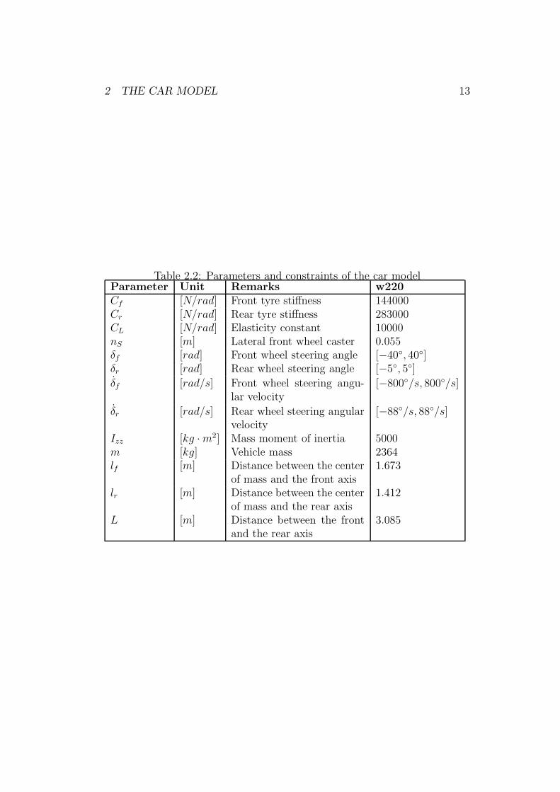
2.3 Model Parameters
The experimental vehicle used is an S-class, and is called Techno Shuttlew220. It has front and rear wheel electro-hydraulic steering, active suspensionand 4 electrohydraulic brakes. The parameters and constraints needed forthe design and in the simulation are given by table 2.2.
With the parameters from table 2.2, and a speed of vx = 14 m/s, thetransfer function of the model is
G =
(
358.9744(s2+7.692s+293)(s2+9.354s+216.8)(s2+6.03s+296.6)
−512.8205(s2+7.692s+205.1)(s2+9.354s+216.8)(s2+6.03s+296.6)
358.9744(s+3.506)(s2+9.354s+216.8)(s2+6.03s+296.6)
−293.0403(s2+9.442s+223.7)(s2+9.354s+216.8)(s2+6.03s+296.6)
)
(2.33)
2 THE CAR MODEL 13
Table 2.2: Parameters and constraints of the car modelParameter Unit Remarks w220Cf [N/rad] Front tyre stiffness 144000Cr [N/rad] Rear tyre stiffness 283000CL [N/rad] Elasticity constant 10000nS [m] Lateral front wheel caster 0.055δf [rad] Front wheel steering angle [−40◦, 40◦]δr [rad] Rear wheel steering angle [−5◦, 5◦]
δf [rad/s] Front wheel steering angu-lar velocity
[−800◦/s, 800◦/s]
δr [rad/s] Rear wheel steering angularvelocity
[−88◦/s, 88◦/s]
Izz [kg ·m2] Mass moment of inertia 5000m [kg] Vehicle mass 2364lf [m] Distance between the center
of mass and the front axis1.673
lr [m] Distance between the centerof mass and the rear axis
1.412
L [m] Distance between the frontand the rear axis
3.085
3 CONTROL STRATEGIES AND SPECIFICATIONS 14
3 Control Strategies and Specifications
3.1 Specifications
When discussing the specifications, there are four main concepts that haveto be mentioned
• Model matching. From the modelled vehicle dynamics, mentioned inthe introduction, the achievement of some particular driving dynamicsis desired. The reference signals are the only interface to the unknownmodel and a good tracking of these references is desired. With this asa starting point, the objective is to make the plant behave just like themodel, and in that way obtain the desired driving dynamics. To achievethis, a plant inverse can be calculated to generate the steering anglescorresponding to the particular reference values. In the ideal situation,i.e. if the plant transfer function is perfectly known, the problem wouldbe solved; the output would always be equal to the reference. But cal-culating the inverse is not a trivial matter, not only because of plantuncertainties. If the plant transfer function has unstable zero dynam-ics and time delays, giving it non-minimum phase characteristics, theinverse would become unstable. This shows the difficulties of obtaininga good inverse. However, an approximate inverse provides a steeringangle reference trajectory, and feedback can be used to stabilise aroundthis nominal trajectory.
• Robustness to system uncertainties. To handle uncertainties of the realplant, a feedback has to be used to handle small excitations of the actualtrajectory from the reference trajectory given by the inverse above.
• Disturbance rejection. Uneven road surface, wind disturbances andinclination of the road are examples of disturbances that can appearand that have to be taken care of by the feedback.
• System integrity. The system has to be stable in all situations. Thismeans that even if one actuator fails, the remaining active controllershould be able to keep the system in stability. In this particular case,the specification is restricted to comprise only rear actuator failure.With a front actuator failure, and the hard constraints on the rearwheel steering angle, a stabilisation would be very hard to achieve.Other factors that might put system integrity to the test, and brakethe feedback loop, could be sensor failure or hitting steering angle con-straints.

3 CONTROL STRATEGIES AND SPECIFICATIONS 15
The closed loop system should have low pass characteristics. It must havea specified closed loop bandwidth (or open loop crossover frequency, whichis almost equivalent), and large enough phase and gain margin to guaranteestability. A high roll-off is needed to achieve good noise reduction, to protectthe actuators and to handle high frequency uncertainties. Furthermore, thedesign has to be resistant to a certain time delay. This will, depending onthe magnitude of the time delay, introduce a reduction in the phase marginof the open loop system. Thus, the damping will decrease, and perhaps thestability will be put at risk as well. Because of this, it is of huge importanceto design the controllers such that the system has enough phase margin andin that way guarantee the system stability. The open loop specifications aregiven in table 3.1.
Table 3.1: Specificationsbandwidth 3 Hz = 18.8 rad/sdamping 0.5time delay 20 ms = 0.020 ssettling time max. 0.5 s
The specified time delay will give a reduction in phase margin (∆φ) by0.020 s · 18.8 rad/s = 0.376 rad = 21 degrees at the crossover frequency. Adamping (D) of 0.5 is equivalent to a phase margin of 51 degrees, accordingto table 3.2 [Burmeister]. By taking the time delay into account, the speci-fication of the phase margin has to be changed from the original 51 degreesto 72 degrees.
Table 3.2: Connection between damping and phase shiftD 0.1 0.2 0.3 0.4 0.5 0.6 0.7 0.8 0.9∆φ 11.4◦ 22.6◦ 33.3◦ 43.1◦ 51.8◦ 59.2◦ 65.2◦ 69.9◦ 73.5◦
3.2 The Feedforward
Although feedforward is the topic of this section, a more general descriptionhas to be made, involving both feedforward and feedback. Some ideas willbe given on how feedforward can be combined with feedback. The feedback,however, will be described more in detail in section 3.3 and in chapter 4.
Attaining a desired system response as specified by a system transferfunction T (s), and simultaneously achieving sufficient feedback to handle

3 CONTROL STRATEGIES AND SPECIFICATIONS 16
uncertainties and disturbances acting on the plant, requires a configurationwith at least two degrees of freedom. The general design paradigm employedhere will be the so called two degree of freedom design. With a referencetrajectory generator, for example the human driver, as the starting point,the objective is to obtain a good trajectory following. From the referencetrajectory, a nominal state space and plant input trajectory is generated usinga full nonlinear plant description. This reference tracking is the first degreeof freedom. The second degree of freedom uses linear theory to deal withdisturbance rejection, stabilisation and robustness to system uncertainties.In this way the problem is divided into one feedforward tracking and onefeedback stabilisation part. Experiments and simulations have shown thatstabilisation around a nominal trajectory allows a more aggressive responsefor nonlinear systems [Nieuwstadt]. The system can be divided in two parts,one linear and one nonlinear. Eventually they will be combined to obtainthe paradigm described above.
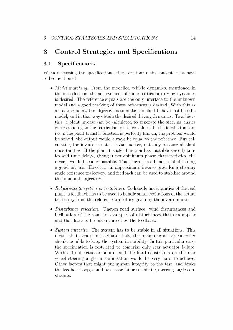
3.2.1 Linear system
Several different structures can be used to describe the two degree of freedomconfiguration. The structure used here is shown in fig 3.1. The significantfeature of any such structure is that the system transfer function T and thesystem sensitivity function S can be independently realised. They fix thevalues of K2 and K1. With
T1(s) = (I +G(s)K1(s)))−1G(s)K1(s) (3.1)
as the closed loop transfer function of the feedback loop and K2 as the feed-forward precompensation, the system equation can be written as
T1(s) ·K2(s) = T (s) =
(
t11(s) t12(s)t21(s) t22(s)
)
(3.2)
and the sensitivity function
S(s) = (1 +G(s)K1(s))−1 (3.3)
The feedforward pre-compensation is used to compensate for the dynam-ics in the feedback loop. Even though a coupling design is used for thefeedback (as will be seen in chapter 4), a significant degree of decoupling isdesired for the system transfer function T . If, for example, a yaw rate anda side slip angle reference is used, it would make sense if the outputs do notcontain any significant cross-coupling with the references; The yaw rate out-put should not depend on the side slip angle reference, and vice versa. The
3 CONTROL STRATEGIES AND SPECIFICATIONS 17
G 1 K −
2 K
Figure 3.1: The two-degree-of-freedom structure.
feedforward compensator can be designed in such a way, that a decouplingis obtained. A K2 that decouples the system would look as follows:
K2(s) = T1(s)−1 ·
(
t11(s) 00 t22(s)
)
(3.4)
However, a pre-compensator like this might be difficult to implement. If itcontains pure derivatives, it would have to be approximated, and the realvalues of K1 and G might differ from the values used in the calculations. Inthe steady state, a pre-compensator is easily obtained. The system steadystate equation would be
T = T1(0) ·K2(0) =
(
1 00 1
)
(3.5)
and a steady state pre-compensator can be calculated. It would give a correcttracking, at least for low frequencies.
3.2.2 Nonlinear system
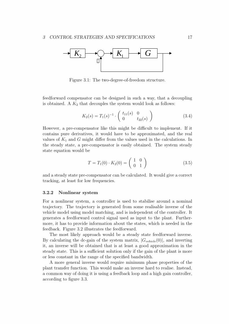
For a nonlinear system, a controller is used to stabilise around a nominaltrajectory. The trajectory is generated from some realisable inverse of thevehicle model using model matching, and is independent of the controller. Itgenerates a feedforward control signal used as input to the plant. Further-more, it has to provide information about the states, which is needed in thefeedback. Figure 3.2 illustrates the feedforward.
The most likely approach would be a steady state feedforward inverse.By calculating the dc-gain of the system matrix, |Gvehicle(0)|, and invertingit, an inverse will be obtained that is at least a good approximation in thesteady state. This is a sufficient solution only if the gain of the plant is moreor less constant in the range of the specified bandwidth.
A more general inverse would require minimum phase properties of theplant transfer function. This would make an inverse hard to realise. Instead,a common way of doing it is using a feedback loop and a high gain controller,according to figure 3.3.
3 CONTROL STRATEGIES AND SPECIFICATIONS 18
ff C R
ref U
Y fb C G
ref ψ ′
ref r , β _
Figure 3.2: Control using feedforward and feedback.
desXR=M o d e l vehicle
GH-
UHigh GainController
Figure 3.3: Feedback loop with high gain controller used to generate thesystem inverse, giving Uref .
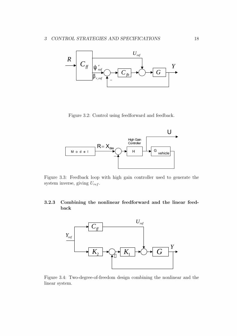
3.2.3 Combining the nonlinear feedforward and the linear feed-back
G 1 K − 2 K
ff C ref U
Y
ref Y
Figure 3.4: Two-degree-of-freedom design combining the nonlinear and thelinear system.

3 CONTROL STRATEGIES AND SPECIFICATIONS 19
A combination of the linear and the nonlinear approach can be doneaccording to figure 3.4 and the problem will be investigated in a linear setting.The feedback loop is used for stabilisation around the nominal trajectory andthe input-output relationship that describes the tracking performance wouldlook according to equation (3.6).
Y = T · Yref = (I +GK1)−1 (GK1K2 +GCff)Yref (3.6)
With some kind of inverse, Cff = G−1, as the starting point, the transferfunction would be
T = (I +GK1)−1(
GK1K2 +GG−1)
= (I +GK1)−1 (GK1K2 +G1) (3.7)
where G1 = GG−1 has low pass characteristics and is some kind of ”approxi-mate” unit matrix. The second factor is the sensitivity function with low gainfor low frequencies. This would give a transfer function for low frequenciesaccording to
Tlowfreq = (I +GK1)−1GK1K2 (3.8)
and allowing a shaping of the feedforward K2 to obtain the desired closedloop characteristics for low frequencies. If the whole frequency spectrum isconsidered, and the feedforward is set to K2 = G1, the transfer function fromreference to output would be
Y = (I +GK1)−1 (GK1G1 +G1)Yref = G1 · Yref (3.9)
This would result in a considerable amount of decoupling (recall that G1 isclose to an unit matrix), and give the system low pass characteristics.
3.3 The Feedback
There are different theories and approaches regarding control of the yaw rateand side slip angle of a car. Here are some of them:
• Decoupling by inverting the system equation and using PD-control (ENT-controller). The integral part in the controller is replaced by a distur-bance observer.
• Decoupling with constraints on the side slip angle. Switching betweenENT- and SM2-controller.
• Independent control of front and rear axle (SM2/BSR). Yaw rate con-trol with the front axle and side slip angle control with the rear axle.

3 CONTROL STRATEGIES AND SPECIFICATIONS 20
• Decoupling through coordinate transformation. Generalisation of thefirst approach.
• Control without using the side slip angle (OBETA).
• Coupling by Individual Channel Design. The design used in this work.Made in the frequency domain, and not in the time domain as theprevious ones. Described in chapter 4.
In previous work, decoupled controllers are used, where system integritycannot be guaranteed. Furthermore, the difficulties of accommodating timedelays and unstructured uncertainties when doing state space design are ex-tensive and have to be mentioned.
The feedback design will be based on the bicycle model from chapter 2.2.Nothing says that this model is a close representation of a real car, mainlybecause of the nonlinear tyre forces that appear when driving a real car,and which are not considered in the model. But in the linear region and forsmall signals the bicycle one track model should be sufficient. The nonlineardifferential system equation is x = f(x, u) and a linearisation can be done intwo ways:
1. Around an equilibrium point, x0, u0, that satisfies f(x0, u0) = 0, or
2. Around a nominal reference trajectory, xref , uref , that satisfies
f(xref , uref) = xref (3.10)
In this particular case, this is a more suitable approach.
Some deviations in the behaviour of the model compared to a real carcan be accepted, on condition that the feedback is designed in such a waythat these uncertainties are suppressed.
There also exist constraints on the steering angles, giving nonlinear actu-ator dynamics. The front actuator is limited to 40 degrees and the rear to 5degrees. If one of them saturates, and an integrator is used in the controller,the resulting windup will cause large overshoots or even make the systemunstable. This is something that has to be taken into consideration whenmaking the design, by constructing an appropriate anti-windup. It is doneaccording to [Astrom], and will not be presented here.
Further, the lightly damped closed loop channel poles change with speed.This implies that the feedback design has to be done for different speeds suchthat the specifications are fulfilled for different driving situations.

4 FEEDBACK - INDIVIDUAL CHANNEL DESIGN 21
4 Coupled Feedback Design with Diagonal Con-
troller - Individual Channel Design
To guarantee the global stability of a car with front wheel steering, or, inother words, preventing it from losing traction, the side slip angle must bekept under control and under a certain threshold. If it exceeds the criticalvalue, the yaw rate control has to be switched to a pure side slip angle control.Simultaneous control of both quantities is impossible with only front wheelsteering. If, instead, a vehicle with both front and rear wheel steering isused, control of both quantities, i.e. the side slip angle and the yaw rate, isenabled.
Individual Channel Design (ICD) will be used for the two-variable feed-back design in the frequency domain. It is an application-oriented design,and it starts from the premise that feedback design is interactive; it involvesan interplay between specifications, uncertain plant characteristics, and themultivariable feedback design process itself. Each of these will be present inthis work, at one point or another.
4.1 Theory
The control approach that is used today is based on decoupled yaw rate andside slip angle controllers, or compensators. This means that one compen-sator, with front wheel steering angle as control signal, is used for controllingthe yaw rate, and another one, with rear wheel steering angle as control sig-nal, controls the side slip angle. The two compensators are designed, in thetime domain, independently of one another, and the mutual interaction isnot considered. Figure 4.1 shows the entire system and it can be seen thatthe yaw rate not only depends on the yaw reference input but also on theside slip angle and vice versa.
This allows us to define a transfer matrix of the plant
G(s) =
(
g11(s) g12(s)g21(s) g22(s)
)
(4.1)
according to equation (2.32), with the reference input and resulting output
R =
(
r1r2
)
=
(
ψref
βr,ref
)
Y =
(
y1
y2
)
=
(
ψβr
)
(4.2)
And the multivariable controller, consisting of two single compensators ki
(i=1,2), can be described by a diagonal matrix
K(s) =
(
k1(s) 00 k2(s)
)
(4.3)

4 FEEDBACK - INDIVIDUAL CHANNEL DESIGN 22
_
_
1 k
2 k
12 g
21 g
22 g
11 g 1 r
2 r
1 u
2 u
1 y
2 y
Figure 4.1: The Complete System
This results in a multivariable feedback loop where an input ui and areference ri can be assigned to each output yi (i=1,2) from the process. Eachcompensator ki uses the output information yi and the reference value ri togive the control signal ui. Under these assumptions one can, without anyloss of information, split this double-input double-output control loop intotwo single-input single-output (SISO) loops, each consisting of a channel, Ci.
For a multivariable system we have, in matrix form, the expression forthe feedback loop
Y = (I −GK)−1GKR = T1R =
(
C1(s)1+C1(s)
g12(s)g22(s)
h2(s)1+C1(s)
g21(s)g11(s)
h1(s)1+C2(s)
C2(s)1+C2(s)
)
R (4.4)
whereCi(s) = ki(s)gii(s) (1 − γ(s)hj(s)) (4.5)
is the open loop SISO transfer function of the channel,
γ(s) =g12(s)g21(s)
g11(s)g22(s)(4.6)
is the complex-frequency multivariable structure function and describes the
4 FEEDBACK - INDIVIDUAL CHANNEL DESIGN 23
internal coupling of the plant, and
hj(s) =kj(s)gjj(s)
1 + kj(s)gjj(s)(4.7)
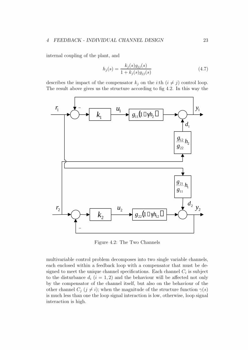
describes the impact of the compensator kj on the i:th (i 6= j) control loop.The result above gives us the structure according to fig 4.2. In this way the
_
_
( ) 2 11 1 h g γ − 1 k
2 k ( ) 12 22 1 h g γ −
2 22
12 h g g
1 r
2 r 2 u
1 u 1 y
2 y
1 11
21 h g g
1 d
2 d
Figure 4.2: The Two Channels
multivariable control problem decomposes into two single variable channels,each enclosed within a feedback loop with a compensator that must be de-signed to meet the unique channel specifications. Each channel Ci is subjectto the disturbance di (i = 1, 2) and the behaviour will be affected not onlyby the compensator of the channel itself, but also on the behaviour of theother channel Cj (j 6= i); when the magnitude of the structure function γ(s)is much less than one the loop signal interaction is low, otherwise, loop signalinteraction is high.

4 FEEDBACK - INDIVIDUAL CHANNEL DESIGN 24
The pole-zero structure of the two channels, assuming that no pole-zerocancellations occur within γ(s), is shown in table 4.1. In equation (4.6) itcan be observed that the poles of g12 and g21 and the zeros of g11 and g22
are the poles of γ(s). However, the zeros of h2 in equation (4.7) includethe zeros of g22 but not g11, which in that case are poles of (1 − γh2), andwill cancel out the zeros of g11 in front of the bracket. Hence, the zeros ofg11 (1 − γh2) are the zeros of (1 − γh2) and the poles of g11 (1 − γh2) are thepoles of g11, g12, g21 and h2. The pole zero structure of C2 is similar.
Table 4.1: Open-loop channel poles and zeros
Zeros Poles
Channel C1 Zeros of (1 − γh2) Poles of g11, g12, g21, h2
Channel C2 Zeros of (1 − γh1) Poles of g22, g12, g21, h1
Individual Channel Design on the original double-input double-outputcross-coupled multivariable system is valid irrespective of the degree of cross-coupling. This extension is shown in [Leithead, O’Reilly].
4.2 Adding Actuators
Second order actuators from equations (2.27a) and (2.27b) are used, withthe transfer functions
Hfront =1
1 +DfTfs+ T 2f s
2(4.8)
Hrear =1
1 +DrTfs+ T 2f s
2(4.9)
and time constant and damping according to table 4.2. The transfer func-tion of the front actuator (equation (4.8)) is multiplied by g11(s) and g21(s)and, similarly, the transfer function of the rear actuator (equation (4.9)) ismultiplied by g22(s) and g12(s). See figure 4.3.
The entire system would be
GPT2 =
(
Hfrontg11 Hrearg12
Hfrontg21 Hrearg22
)
(4.10)

4 FEEDBACK - INDIVIDUAL CHANNEL DESIGN 25
Table 4.2: Actuator parameters.
Time constant T (s) Damping D (s)
Front actuator 0.012 0.612Rear actuator 0.0072 0.612
12 g
21 g
22 g
11 g 1 u
2 u
1 y
2 y Rear actuator
Front actuator
Figure 4.3: The connection between the plant and the actuators
4.3 The Main Advantages and Disadvantages
As mentioned in the introduction, the control system has to be robust toplant uncertainties, and a failure of one actuator must not destabilise thesystem. The actuators are connected to the plant according to figure 4.3. Itshould be recalled that the open loop transmittance C1 is the transmittancebetween r1 and y1, with the feedback loop from plant output 1 to controlinput 1 open, but with the other feedback loop closed. And likewise forchannel 2. Hence, a failure of one actuator means that the feedback loopof the channel Ci, which the actuator concerned belongs to, is broken. Thesubsystem transfer function in question, hi, can be set equal to zero. The

4 FEEDBACK - INDIVIDUAL CHANNEL DESIGN 26
other channel will, consequently, have a rather simple structure:
Cj(s) = kj(s)gjj(s) (i 6= j) (4.11)
and it is of great importance to make sure that the remaining active com-pensator, kj, can stabilise the system. The performance, and in particularthe stability, of the closed loop system under a failure of one of the feedbackloops may thus be determined directly from inspection of the poles of thecorresponding open loop channel transmittance. In other words, system in-tegrity after feedback loop failure is guaranteed provided the following twoconditions are satisfied:
1. all the individual plant transfer functions gij(s) (i, j = 1, 2), are stable;
2. the subsystem transfer functions hi(s) (i = 1, 2), are stable.
With the decoupled system, this would not be self-evident.When designing the controller for a plant, one of the primary requirements
is robustness; that is, to ensure that the resulting closed loop performanceis not badly degraded by plant uncertainty. This is done by designing con-trollers such that sufficiently large phase and gain margins are obtained toguarantee satisfactory closed loop performance even in the presence of plantuncertainties. But, this is only valid in the SISO case. For a double-inputdouble-output system, enough phase and gain margins are not sufficient forrobustness to plant uncertainties. There are two reasons for that: excessivephase/structural sensitivity to plant parameter uncertainty at frequenciesat/below the channel crossover frequency. This leads to the following addi-tional requirement [Leithead,O’Reilly]:
• For robustness of the closed loop system stability to general plant pa-rameter uncertainty, it is necessary that the Nyquist plots of the multi-variable structure functions γhi(s) (i = 1, 2) do not go close to the point(1,0) at frequencies near or less than the channel crossover frequencies.
In the requirement above, large plant uncertainty is implicitly assumed.When the plant is well known, single-loop control can be used with thedecoupled system.
The feedback design is carried out in the frequency domain. The conver-sion from state space representation to transfer function means that infor-mation about the internal structure of the plant is lost. Furthermore, thedesign is restricted to the linear region.
4 FEEDBACK - INDIVIDUAL CHANNEL DESIGN 27
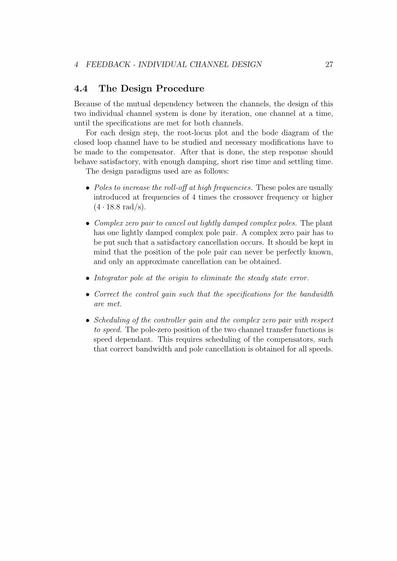
4.4 The Design Procedure
Because of the mutual dependency between the channels, the design of thistwo individual channel system is done by iteration, one channel at a time,until the specifications are met for both channels.
For each design step, the root-locus plot and the bode diagram of theclosed loop channel have to be studied and necessary modifications have tobe made to the compensator. After that is done, the step response shouldbehave satisfactory, with enough damping, short rise time and settling time.
The design paradigms used are as follows:
• Poles to increase the roll-off at high frequencies. These poles are usuallyintroduced at frequencies of 4 times the crossover frequency or higher(4 · 18.8 rad/s).
• Complex zero pair to cancel out lightly damped complex poles. The planthas one lightly damped complex pole pair. A complex zero pair has tobe put such that a satisfactory cancellation occurs. It should be kept inmind that the position of the pole pair can never be perfectly known,and only an approximate cancellation can be obtained.
• Integrator pole at the origin to eliminate the steady state error.
• Correct the control gain such that the specifications for the bandwidthare met.
• Scheduling of the controller gain and the complex zero pair with respectto speed. The pole-zero position of the two channel transfer functions isspeed dependant. This requires scheduling of the compensators, suchthat correct bandwidth and pole cancellation is obtained for all speeds.

5 FEEDBACK DESIGN - RESULTS 28
5 Feedback Design - Results
The second order actuators have high frequency poles with low damping.Just cancelling the actuators poles by zeros would be unrealistic since thelightly damped poles move with changing actuator parameters. Instead, anapproach with no actuator cancellation can be used (according to section4.4):
k1 =K1 (s− z1) (s− z∗1)
s (s+ 80)(5.1)
k2 =K2 (s− z2) (s− z∗2)
s (s+ 80)(5.2)
The dominant pole structure of the plant looks according to figure 5.1.After a few iterations, by placing the compensator complex zero right on the
−18 −16 −14 −12 −10 −8 −6 −4 −2−20
−15
−10
−5
0
5
10
15
20
Re
Im
Poles as speed changes from 5 to 30 m/s
vx=5m/s
vx=30m/s
vx=5m/s
vx=30m/s
Figure 5.1: Poles of the plant as a function of speed
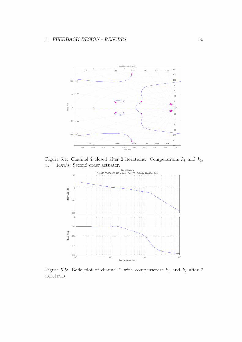
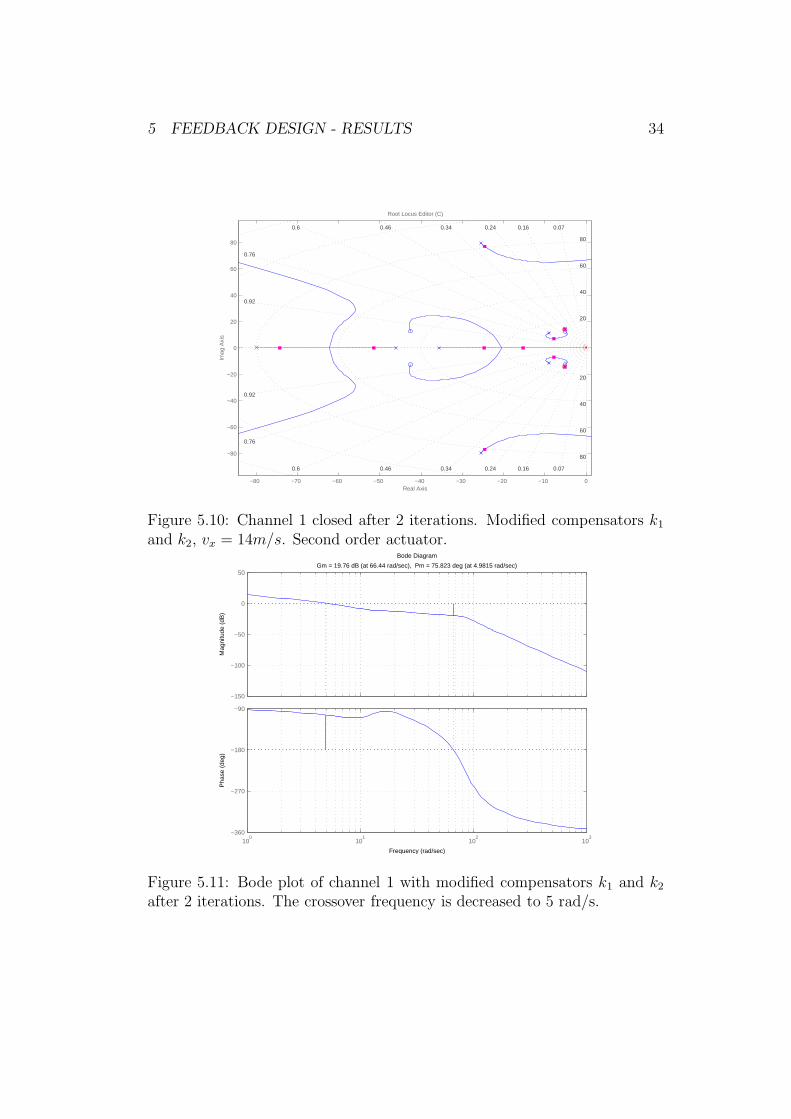
lightly damped complex pole of the plant and adjusting the gain to get thespecified bandwidth, the zero-gain structure in table 5.1 and the root-locusplots and bode diagrams in figures 5.2 to 5.5, are obtained. The speed isvx = 14m/s.
The phase margins and cross-over frequencies are shown in table 5.2.In the bode plot of the first channel (figure 5.3), a plateau around the
frequencies of the controller complex zero (15 rad/s) can be observed. The

5 FEEDBACK DESIGN - RESULTS 29
−80 −70 −60 −50 −40 −30 −20 −10 0
−80
−60
−40
−20
0
20
40
60
80
20
0.94
0.8
0.64
0.08
80
0.28
0.5
40
0.38
40
0.28
0.17
0.17 0.08
0.94
20
0.8
60
0.6480
0.5 0.38
60
Real Axis
Root Locus Editor (C)Im
ag A
xis
Figure 5.2: Channel 1 closed after 2 iterations. Compensators k1 and k2,vx = 14m/s. Second order actuator.
Bode Diagram
Frequency (rad/sec)
Pha
se (
deg)
Mag
nitu
de (
dB)
−100
−50
0
50Gm = 7.4195 dB (at 66.44 rad/sec), Pm = 83.843 deg (at 18.3 rad/sec)
100
101
102
103
−360
−270
−180
−90
Figure 5.3: Bode plot of channel 1 with compensators k1 and k2 after 2iterations.
5 FEEDBACK DESIGN - RESULTS 30
−90 −80 −70 −60 −50 −40 −30 −20 −10 0
−100
−50
0
50
100
140
120
100
80
20
0.38 0.06
100
60
0.2
40
20
140
0.88
0.7
0.52
0.52
0.28
0.38
0.13
0.28 0.2
80
0.13
120
0.06
60
0.88
0.7
40
Real Axis
Root Locus Editor (C)Im
ag A
xis
Figure 5.4: Channel 2 closed after 2 iterations. Compensators k1 and k2,vx = 14m/s. Second order actuator.
Bode Diagram
Frequency (rad/sec)
Pha
se (
deg)
Mag
nitu
de (
dB)
−100
−50
0
50Gm = 15.37 dB (at 96.459 rad/sec), Pm = 85.12 deg (at 17.855 rad/sec)
100
101
102
103
−360
−270
−180
−90
0
Figure 5.5: Bode plot of channel 2 with compensators k1 and k2 after 2iterations.
5 FEEDBACK DESIGN - RESULTS 31
Step Response
Time (sec)
Am
plitu
de
0 0.1 0.2 0.3 0.4 0.5 0.6 0.7 0.8 0.9 10
0.2
0.4
0.6
0.8
1
1.2
1.4
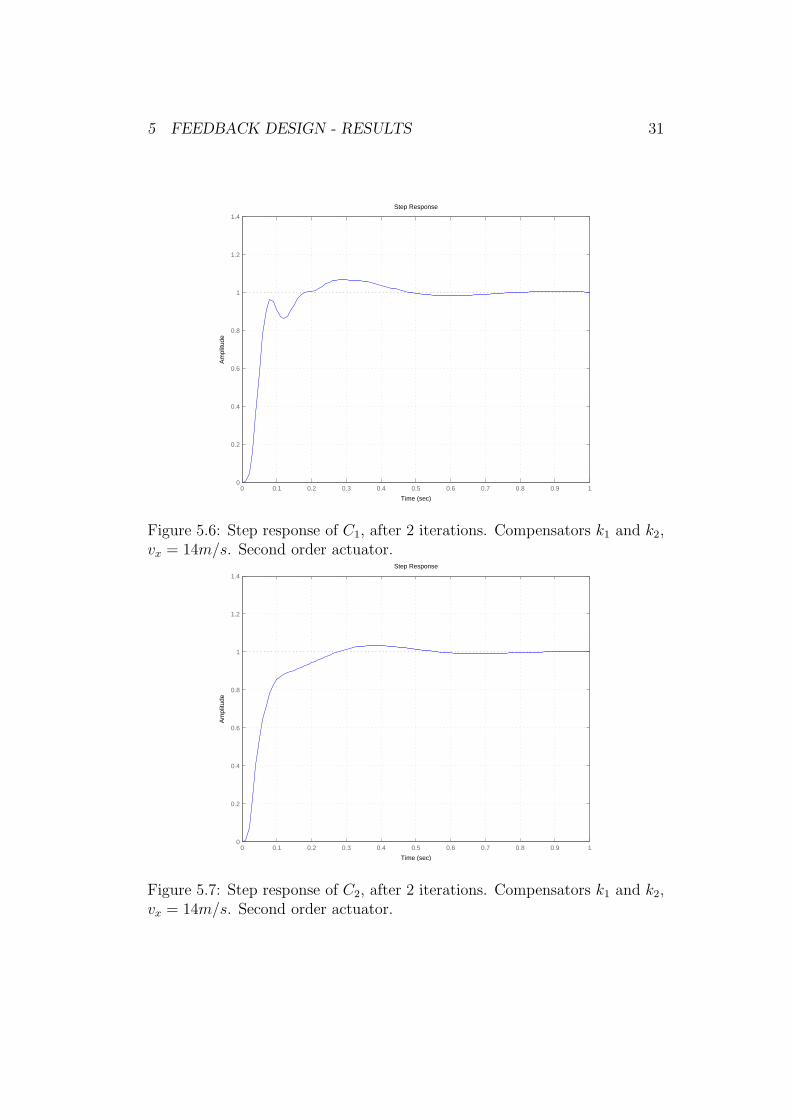
Figure 5.6: Step response of C1, after 2 iterations. Compensators k1 and k2,vx = 14m/s. Second order actuator.
Step Response
Time (sec)
Am
plitu
de
0 0.1 0.2 0.3 0.4 0.5 0.6 0.7 0.8 0.9 10
0.2
0.4
0.6
0.8
1
1.2
1.4
Figure 5.7: Step response of C2, after 2 iterations. Compensators k1 and k2,vx = 14m/s. Second order actuator.
5 FEEDBACK DESIGN - RESULTS 32
Impulse Response
Time (sec)
Am
plitu
de
0 0.1 0.2 0.3 0.4 0.5 0.6 0.7 0.8 0.9 1−5
0
5
10
15
20
25
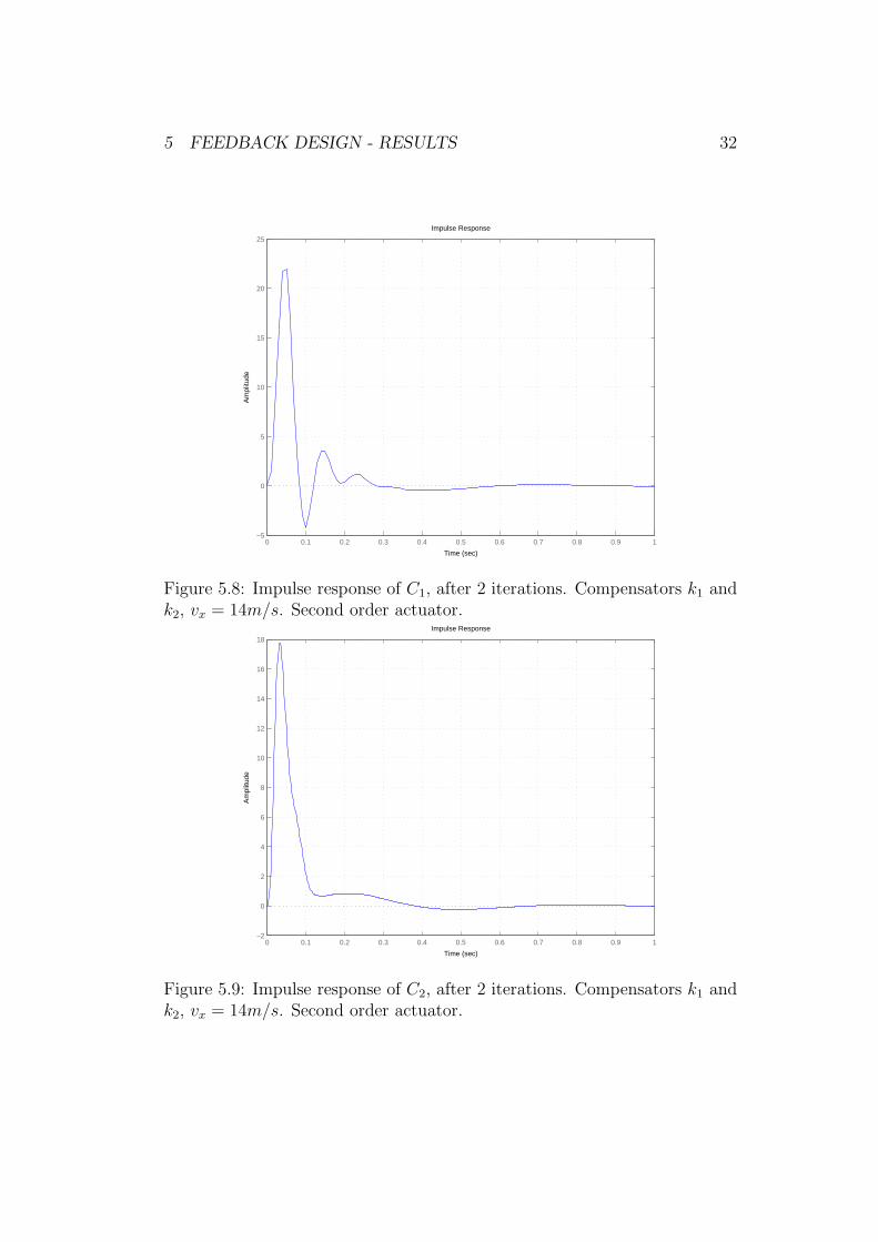
Figure 5.8: Impulse response of C1, after 2 iterations. Compensators k1 andk2, vx = 14m/s. Second order actuator.
Impulse Response
Time (sec)
Am
plitu
de
0 0.1 0.2 0.3 0.4 0.5 0.6 0.7 0.8 0.9 1−2
0
2
4
6
8
10
12
14
16
18
Figure 5.9: Impulse response of C2, after 2 iterations. Compensators k1 andk2, vx = 14m/s. Second order actuator.

5 FEEDBACK DESIGN - RESULTS 33
Table 5.1: Gain, and complex zero pair, of the two compensators with secondorder actuator and vx = 14.
Gain Ki (i = 1, 2) Zero zi (i = 1, 2)
Channel C1 2.4692 −5.1780 + 14.1772iChannel C2 -5.8253 −5.1780 + 14.1772i
Table 5.2: Phase margin and crossover frequency of both channels, withsecond order actuator and vx = 14.
Phase margin, ∆φ Cross-over frequency (rad/s)
Channel C1 84◦ 18.3Channel C2 85◦ 17.9
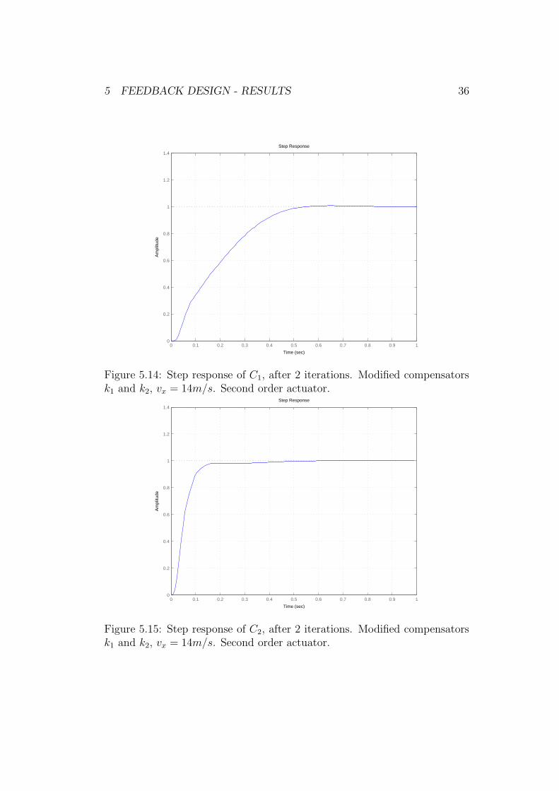
gain there is only 1.07 (0.6dB), which might aggravate the closed loop per-formance in terms of noise rejection around those frequencies. Furthermore,the slightest uncertainty in compensator gain might change the crossover fre-quency and phase margin significantly. The gain margin of the first channelis also very low. This gives, as can be seen in figure 5.6, lightly dampedmodes in the step response, caused by bad damping of the actuator poles.If the specifications are relaxed for the first channel, by allowing a lowerbandwidth, this problem can be solved with a modified first compensator.There will be a loss in performance, but in this case a tradeoff has to be donebetween entirely meeting the specifications and having a high performance.The resulting zero-gain structure, root-locus plot and bode diagram of thetwo channels, after two iterations, are shown in table 5.3 and figures 5.10 to5.13. The decreased performance of channel 1 compared to channel 2 canbe seen in the step and impulse responses in figures 5.14 to 5.17. Table 5.4shows the phase margins and crossover frequencies. The closed loop gain forfrequencies within the bandwidth has to be close to 1 for both channels. Thisis illustrated in figures 5.18 and 5.19.
Many different solutions for design have been tried out, and the function-
5 FEEDBACK DESIGN - RESULTS 34
−80 −70 −60 −50 −40 −30 −20 −10 0
−80
−60
−40
−20
0
20
40
60
80
20
0.92
0.76
0.6
0.07
80
0.24
0.46
40
0.34
40
0.24
0.16
0.16 0.07
0.92
20
0.76
60
0.6
80
0.46 0.34
60
Real Axis
Root Locus Editor (C)Im
ag A
xis
Figure 5.10: Channel 1 closed after 2 iterations. Modified compensators k1
and k2, vx = 14m/s. Second order actuator.Bode Diagram
Frequency (rad/sec)
Pha
se (
deg)
Mag
nitu
de (
dB)
−150
−100
−50
0
50Gm = 19.76 dB (at 66.44 rad/sec), Pm = 75.823 deg (at 4.9815 rad/sec)
100
101
102
103
−360
−270
−180
−90
Figure 5.11: Bode plot of channel 1 with modified compensators k1 and k2
after 2 iterations. The crossover frequency is decreased to 5 rad/s.

5 FEEDBACK DESIGN - RESULTS 35
−80 −70 −60 −50 −40 −30 −20 −10 0
−100
−50
0
50
100
140
120
100
80
0.66
0.36 0.06
80
60
0.18
40
20
120
0.86
0.66
0.48
0.48
0.26
0.36
0.11
0.26 0.18
60
0.11
100
0.06
20
0.86
40
Real Axis
Root Locus Editor (C)Im
ag A
xis
Figure 5.12: Channel 2 closed after 2 iterations. Modified compensators k1
and k2, vx = 14m/s. Second order actuator.Bode Diagram
Frequency (rad/sec)
Pha
se (
deg)
Mag
nitu
de (
dB)
−100
−50
0
50Gm = 15.305 dB (at 96.528 rad/sec), Pm = 71.697 deg (at 18.06 rad/sec)
100
101
102
103
−360
−270
−180
−90
Figure 5.13: Bode plot of channel 2 with modified compensators k1 and k2
after 2 iterations.
5 FEEDBACK DESIGN - RESULTS 36
Step Response
Time (sec)
Am
plitu
de
0 0.1 0.2 0.3 0.4 0.5 0.6 0.7 0.8 0.9 10
0.2
0.4
0.6
0.8
1
1.2
1.4
Figure 5.14: Step response of C1, after 2 iterations. Modified compensatorsk1 and k2, vx = 14m/s. Second order actuator.
Step Response
Time (sec)
Am
plitu
de
0 0.1 0.2 0.3 0.4 0.5 0.6 0.7 0.8 0.9 10
0.2
0.4
0.6
0.8
1
1.2
1.4
Figure 5.15: Step response of C2, after 2 iterations. Modified compensatorsk1 and k2, vx = 14m/s. Second order actuator.
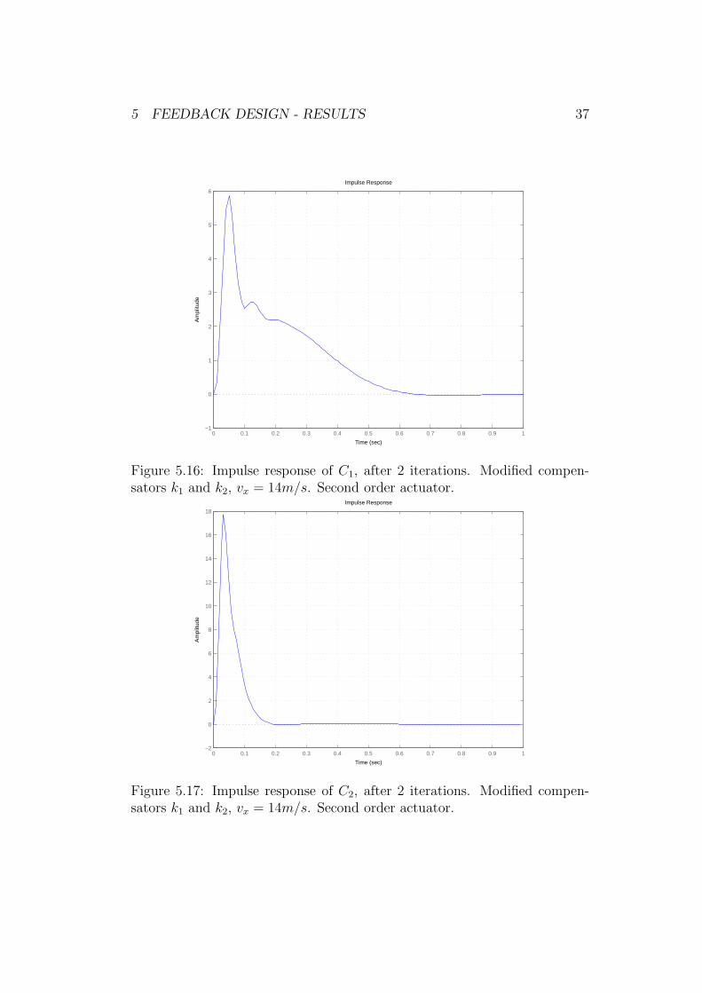
5 FEEDBACK DESIGN - RESULTS 37
Impulse Response
Time (sec)
Am
plitu
de
0 0.1 0.2 0.3 0.4 0.5 0.6 0.7 0.8 0.9 1−1
0
1
2
3
4
5
6
Figure 5.16: Impulse response of C1, after 2 iterations. Modified compen-sators k1 and k2, vx = 14m/s. Second order actuator.
Impulse Response
Time (sec)
Am
plitu
de
0 0.1 0.2 0.3 0.4 0.5 0.6 0.7 0.8 0.9 1−2
0
2
4
6
8
10
12
14
16
18
Figure 5.17: Impulse response of C2, after 2 iterations. Modified compen-sators k1 and k2, vx = 14m/s. Second order actuator.

5 FEEDBACK DESIGN - RESULTS 38
Bode Diagram
Frequency (rad/sec)
Pha
se (
deg)
Mag
nitu
de (
dB)
100
101
102
103
−360
−315
−270
−225
−180
−135
−90
−45
0
−120
−100
−80
−60
−40
−20
0
Figure 5.18: Bode plot of first loop closed with modified compensators k1
and k2 after 2 iterations.Bode Diagram
Frequency (rad/sec)
Pha
se (
deg)
Mag
nitu
de (
dB)
−100
−80
−60
−40
−20
0
100
101
102
103
−360
−270
−180
−90
0
Figure 5.19: Bode plot of second loop closed with modified compensators k1
and k2 after 2 iterations.

5 FEEDBACK DESIGN - RESULTS 39
Table 5.3: Gain, and complex zero pair, of the two compensators with secondorder actuator and vx = 14.
Gain Ki (i = 1, 2) Zero zi (i = 1, 2)
Channel C1 0.5964 −5.1780 + 14.1772iChannel C2 -5.8253 −5.1780 + 14.1772i
Table 5.4: Phase margin and crossover frequency of both channels, withsecond order actuator and vx = 14. Modified compensators.
Phase margin, ∆φ Cross-over frequency (rad/s)
Channel C1 76◦ 4.98Channel C2 72◦ 18.1
ality is shown to be very sensitive to changes in tyre parameters. A notchfilter can be used with the first compensator to get rid of the plateau, and ahigher bandwidth might then be allowed. An additional complex pole pair,in addition to the complex zero pair already used, has been tried out. Thiswould pull the lightly damped complex pole pair towards the left in the com-plex plane and increase the damping of that pole. However, the open loopphase margin would decrease significantly, with a resulting loss in robustness,which has been proved in simulations.
5.1 Controller Scheduling
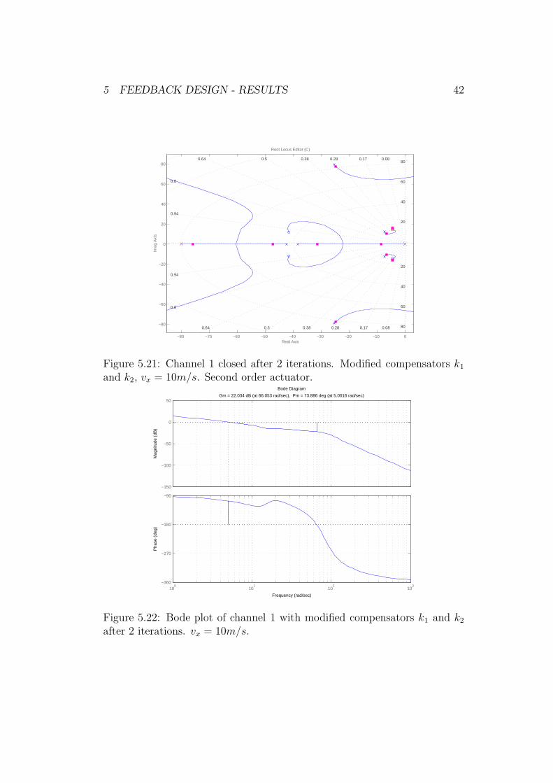
The design in the previous section was made with speed 14 m/s, by placinga zero right on the most lightly damped pole of the open system. But, thesystem must have the same closed loop characteristics for all speeds that canbe reached with normal driving. The bandwidth has to be maintained andphase margin has to remain above the specified value. Too low speeds donot cause any need for feedback, and the interesting speeds in this case arefrom 5 m/s to 30 m/s. Figure 5.20 shows how the most lightly damped pole

5 FEEDBACK DESIGN - RESULTS 40
varies with longitudinal speed.
−10 −9 −8 −7 −6 −5 −4 −3 −2 −1 00
2
4
6
8
10
12
14
16
18
20
Re
ImLightly damped pole as speed changes from 5 to 30 m/s
vx=5m/s
vx=30m/s
Figure 5.20: Most lightly damped open loop pole as a function of speed
This implies that the compensators have to be adapted continuously withrespect to speed. First, the complex zero pair must be placed on the lightlydamped pole, according to figure 5.20. Then, a gain scheduling has to be doneto obtain the specified crossover frequency (5 rad/s for channel 1 and 18 rad/s for channel 2). The transfer function of the first channel, C1, is calculated.Since the bandwidth of channel 1 is small in comparison to channel 2, thetransfer function h2 can be set to 1, and C1 can easily be calculated. Now,the gain at the desired crossover frequency, i.e. 5 rad/s, is evaluated, andinverted, which will give the correct gain of the first compensator. Once thiscompensator is determined, h1 and C2 can easily be calculated. The gainat 18 rad/s is evaluated, and an inversion will give the gain of the secondcompensator. How the scheduling is carried out in practice is shown in theappendix.
Figures 5.21 to 5.36 show the root locus plots, bode plots, step and im-pulse responses, for both channels, and for speeds 10 m/s and 25 m/s, afterfollowing the above mentioned scheduling procedure. In figure 5.37, the bodeplot of the first channel, with speeds between 5 m/s to 25 m/s, is illustrated.For lower speeds, the roll-off around the frequencies of the controller zero isconsiderably higher than for high speeds. Furthermore, a higher gain marginis also observed for low speeds. This means that the system shows a much

5 FEEDBACK DESIGN - RESULTS 41
better noise rejection for low than for high speeds. On the other hand, thephase margin decreases for lower speeds, as shown in table 5.5. This resultsin lower damping and a more oscillatory behaviour, which is never an issuefor high speeds. For the second channel, the behaviour is rather similar forall speeds (figure 5.38), and, above all, much faster than for the first channel,mainly due to the higher gain giving a higher crossover frequency. In general,the system seems to have a faster behaviour for low speeds, but also a largersettling time, which can be seen in the closed loop step and impulse responsesin figures 5.39 to 5.42. The faster and more oscillatory characteristics for lowspeeds can be explained by studying the root-locus plot of the first channel,for a low and a high speed respectively, as in figures 5.21 and 5.29. For thelower speed (10 m/s, fig. 5.21), a not completely out-cancelled pole withdamping 0.5 is present, while for the higher speed (25 m/s, fig. 5.29), thedamping is much greater, 0.8. The actuator pole is badly damped, but itshigh frequency makes the impact on the channel negligible.
The specifications that were put up for phase margin, are, as can beseen in table 5.5, precisely met. The specified step response and impulsenoise rejection settling time of 0.5 s, is, according to figures 5.39 to 5.42,reached for both channels (the definition of settling time can be found in thelitterature). However, the settling time is much longer for channel 1.
Table 5.5: Phase margin of both channels, with second order actuator, andfor different speeds. Modified compensators.
25 m/s 21 m/s 18 m/s 14 m/s 10 m/s 5 m/s
Channel C1 92.4◦ 85.1◦ 80.6◦ 75.8◦ 73.9◦ 76.5◦
Channel C2 79.7◦ 75.6◦ 73.7◦ 71.7◦ 71.4◦ 72.2◦
5.2 System Integrity and Robustness
In this section, system integrity and robustness to plant uncertainties arestudied. We recall from section 4.3 that determining system integrity is doneby inspection of the poles of C1 and C2.
1. Figure 5.1 shows that the plant transfer matrix has no right half planepoles. These poles are equivalent to the poles of the individual planttransfer functions gij(s), i, j = 1, 2 [Maciejowski].
5 FEEDBACK DESIGN - RESULTS 42
−80 −70 −60 −50 −40 −30 −20 −10 0
−80
−60
−40
−20
0
20
40
60
80
20
0.94
0.8
0.64
0.08
80
0.28
0.5
40
0.38
40
0.28
0.17
0.17 0.08
0.94
20
0.8
60
0.6480
0.5 0.38
60
Real Axis
Root Locus Editor (C)Im
ag A
xis
Figure 5.21: Channel 1 closed after 2 iterations. Modified compensators k1
and k2, vx = 10m/s. Second order actuator.Bode Diagram
Frequency (rad/sec)
Pha
se (
deg)
Mag
nitu
de (
dB)
−150
−100
−50
0
50Gm = 22.034 dB (at 66.053 rad/sec), Pm = 73.886 deg (at 5.0016 rad/sec)
100
101
102
103
−360
−270
−180
−90
Figure 5.22: Bode plot of channel 1 with modified compensators k1 and k2
after 2 iterations. vx = 10m/s.

5 FEEDBACK DESIGN - RESULTS 43
−90 −80 −70 −60 −50 −40 −30 −20 −10 0
−100
−50
0
50
100
140
120
100
80
20
0.38 0.06
100
60
0.19
40
20
140
0.88
0.68
0.52
0.52
0.28
0.38
0.12
0.28 0.19
80
0.12
120
0.06
60
0.88
0.68
40
Real Axis
Root Locus Editor (C)Im
ag A
xis
Figure 5.23: Channel 2 closed after 2 iterations. Modified compensators k1
and k2, vx = 10m/s. Second order actuator.Bode Diagram
Frequency (rad/sec)
Pha
se (
deg)
Mag
nitu
de (
dB)
−100
−50
0
50Gm = 15.078 dB (at 96.587 rad/sec), Pm = 71.4 deg (at 18.137 rad/sec)
100
101
102
103
−360
−270
−180
−90
Figure 5.24: Bode plot of channel 2 with modified compensators k1 and k2
after 2 iterations. vx = 10m/s.

5 FEEDBACK DESIGN - RESULTS 44
Step Response
Time (sec)
Am
plitu
de
0 0.1 0.2 0.3 0.4 0.5 0.6 0.7 0.8 0.9 10
0.1
0.2
0.3
0.4
0.5
0.6
0.7
0.8
0.9
1
Figure 5.25: Step response of C1, after 2 iterations. Modified compensatorsk1 and k2, vx = 10m/s. Second order actuator.
Step Response
Time (sec)
Am
plitu
de
0 0.1 0.2 0.3 0.4 0.5 0.6 0.7 0.8 0.9 10
0.2
0.4
0.6
0.8
1
1.2
1.4
Figure 5.26: Step response of C2, after 2 iterations. Modified compensatorsk1 and k2, vx = 10m/s. Second order actuator.

5 FEEDBACK DESIGN - RESULTS 45
Impulse Response
Time (sec)
Am
plitu
de
0 0.1 0.2 0.3 0.4 0.5 0.6 0.7 0.8 0.9 1−1
0
1
2
3
4
5
Figure 5.27: Impulse response of C1, after 2 iterations. Modified compen-sators k1 and k2, vx = 10m/s. Second order actuator.
Impulse Response
Time (sec)
Am
plitu
de
0 0.1 0.2 0.3 0.4 0.5 0.6 0.7 0.8 0.9 1−5
0
5
10
15
20
Figure 5.28: Impulse response of C2, after 2 iterations. Modified compen-sators k1 and k2, vx = 10m/s. Second order actuator.
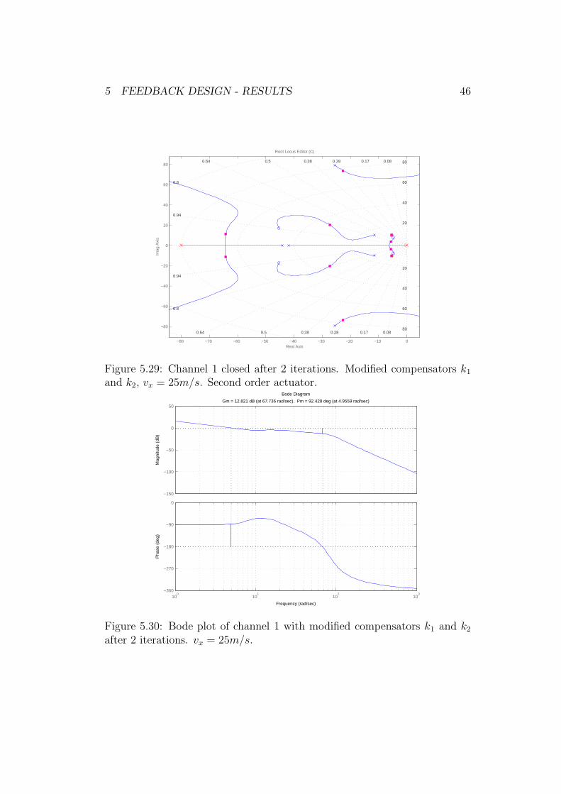
5 FEEDBACK DESIGN - RESULTS 46
−80 −70 −60 −50 −40 −30 −20 −10 0
−80
−60
−40
−20
0
20
40
60
80
20
0.94
0.8
0.64
0.08
80
0.28
0.5
40
0.38
40
0.28
0.17
0.17 0.08
0.94
20
0.8
60
0.64 800.5 0.38
60
Real Axis
Root Locus Editor (C)Im
ag A
xis
Figure 5.29: Channel 1 closed after 2 iterations. Modified compensators k1
and k2, vx = 25m/s. Second order actuator.Bode Diagram
Frequency (rad/sec)
Pha
se (
deg)
Mag
nitu
de (
dB)
−150
−100
−50
0
50Gm = 12.821 dB (at 67.736 rad/sec), Pm = 92.428 deg (at 4.9559 rad/sec)
100
101
102
103
−360
−270
−180
−90
0
Figure 5.30: Bode plot of channel 1 with modified compensators k1 and k2
after 2 iterations. vx = 25m/s.
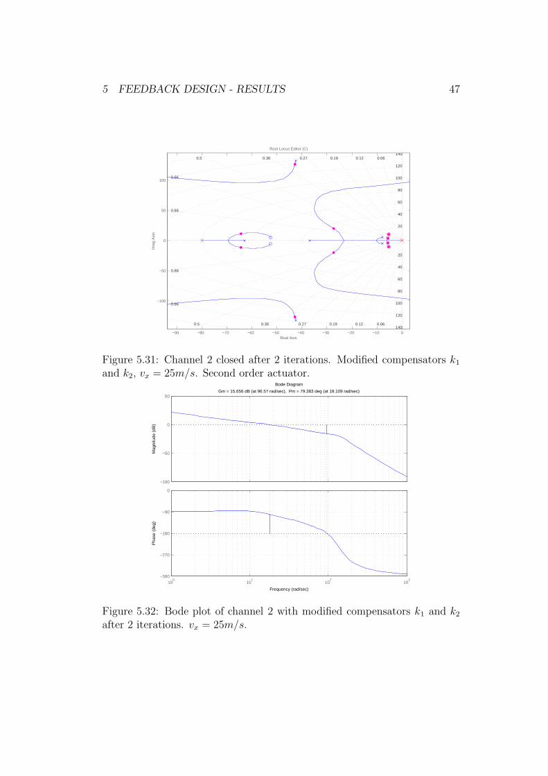
5 FEEDBACK DESIGN - RESULTS 47
−90 −80 −70 −60 −50 −40 −30 −20 −10 0
−100
−50
0
50
100
140
120
100
80
20
0.19 0.06
100
0.36
60
40
20
140
0.88
0.5
0.66
0.27
0.5
0.12
0.36 0.27 0.19
80
0.12
120
0.06
60
0.88
0.66
40
Real Axis
Root Locus Editor (C)Im
ag A
xis
Figure 5.31: Channel 2 closed after 2 iterations. Modified compensators k1
and k2, vx = 25m/s. Second order actuator.Bode Diagram
Frequency (rad/sec)
Pha
se (
deg)
Mag
nitu
de (
dB)
−100
−50
0
50Gm = 15.656 dB (at 96.57 rad/sec), Pm = 79.383 deg (at 18.109 rad/sec)
100
101
102
103
−360
−270
−180
−90
0
Figure 5.32: Bode plot of channel 2 with modified compensators k1 and k2
after 2 iterations. vx = 25m/s.
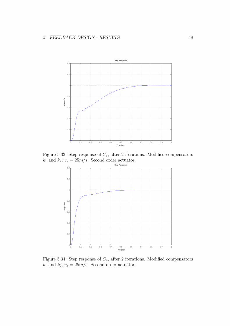
5 FEEDBACK DESIGN - RESULTS 48
Step Response
Time (sec)
Am
plitu
de
0 0.1 0.2 0.3 0.4 0.5 0.6 0.7 0.8 0.9 10
0.2
0.4
0.6
0.8
1
1.2
1.4
Figure 5.33: Step response of C1, after 2 iterations. Modified compensatorsk1 and k2, vx = 25m/s. Second order actuator.
Step Response
Time (sec)
Am
plitu
de
0 0.1 0.2 0.3 0.4 0.5 0.6 0.7 0.8 0.9 10
0.2
0.4
0.6
0.8
1
1.2
1.4
Figure 5.34: Step response of C2, after 2 iterations. Modified compensatorsk1 and k2, vx = 25m/s. Second order actuator.
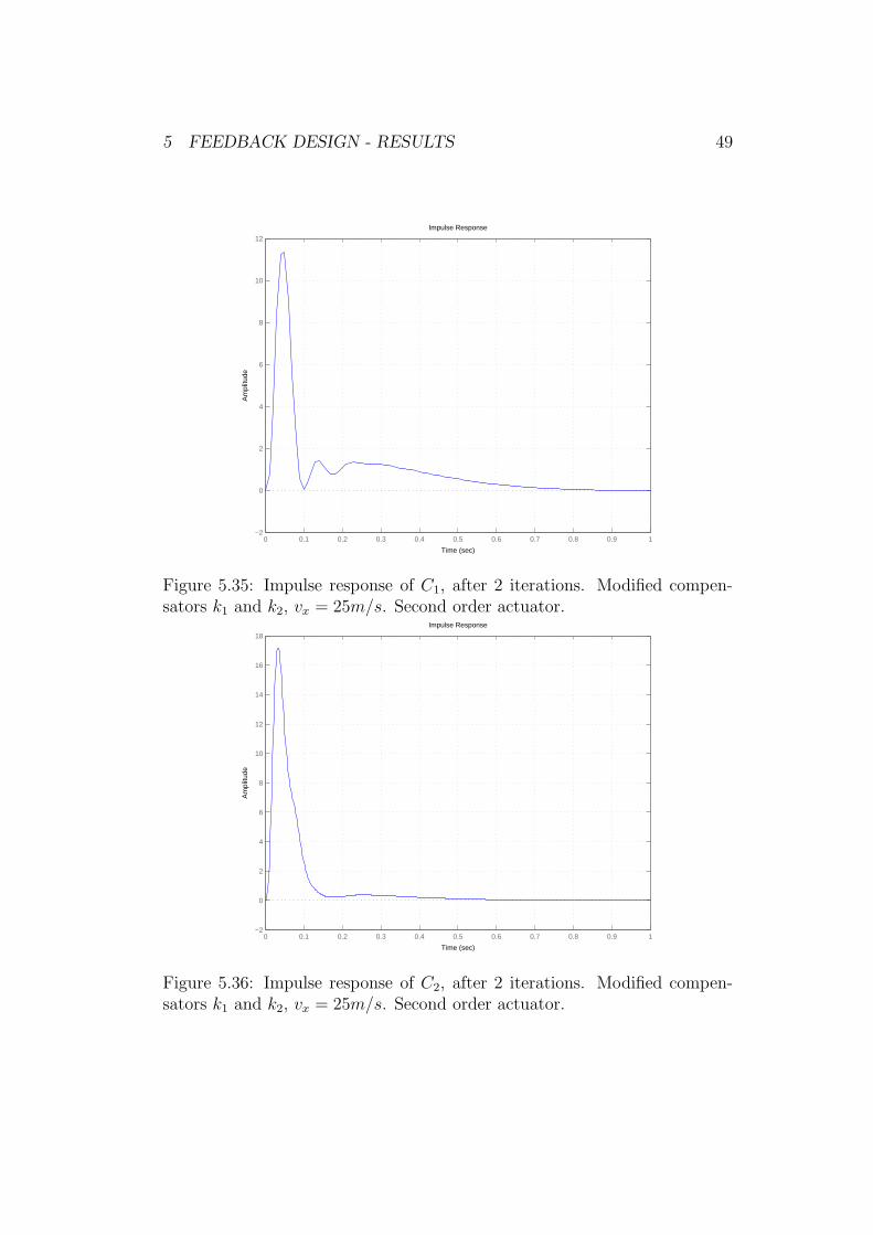
5 FEEDBACK DESIGN - RESULTS 49
Impulse Response
Time (sec)
Am
plitu
de
0 0.1 0.2 0.3 0.4 0.5 0.6 0.7 0.8 0.9 1−2
0
2
4
6
8
10
12
Figure 5.35: Impulse response of C1, after 2 iterations. Modified compen-sators k1 and k2, vx = 25m/s. Second order actuator.
Impulse Response
Time (sec)
Am
plitu
de
0 0.1 0.2 0.3 0.4 0.5 0.6 0.7 0.8 0.9 1−2
0
2
4
6
8
10
12
14
16
18
Figure 5.36: Impulse response of C2, after 2 iterations. Modified compen-sators k1 and k2, vx = 25m/s. Second order actuator.

5 FEEDBACK DESIGN - RESULTS 50
Bode Diagram
Frequency (rad/sec)
Pha
se (
deg)
Mag
nitu
de (
dB)
−150
−100
−50
0
50speed 5 m/sspeed 10 m/sspeed 14 m/sspeed 18 m/sspeed 21 m/sspeed 25 m/s
100
101
102
103
−360
−270
−180
−90
0
Figure 5.37: Bode plot of channel 1 for different speeds with modified com-pensators k1 and k2 after 2 iterations.
Bode Diagram
Frequency (rad/sec)
Pha
se (
deg)
Mag
nitu
de (
dB)
−100
−50
0
50speed 5 m/sspeed 10 m/sspeed 14 m/sspeed 18 m/sspeed 21 m/sspeed 25 m/s
100
101
102
103
−360
−270
−180
−90
0
Figure 5.38: Bode plot of channel 2 for different speeds with modified com-pensators k1 and k2 after 2 iterations.

5 FEEDBACK DESIGN - RESULTS 51
Step Response
Time (sec)
Am
plitu
de
0 0.1 0.2 0.3 0.4 0.5 0.6 0.7 0.8 0.9 10
0.2
0.4
0.6
0.8
1
1.2
1.4speed 5 m/sspeed 10 m/sspeed 14 m/sspeed 18 m/sspeed 21 m/sspeed 25 m/s
Figure 5.39: Step response of C1, after 2 iterations, for different speeds.Modified compensators k1 and k2. Second order actuator.
Step Response
Time (sec)
Am
plitu
de
0 0.1 0.2 0.3 0.4 0.5 0.6 0.7 0.8 0.9 10
0.2
0.4
0.6
0.8
1
1.2
1.4speed 5 m/sspeed 10 m/sspeed 14 m/sspeed 18 m/sspeed 21 m/sspeed 25 m/s
Figure 5.40: Step response of C2, after 2 iterations, for different speeds.Modified compensators k1 and k2. Second order actuator.

5 FEEDBACK DESIGN - RESULTS 52
Impulse Response
Time (sec)
Am
plitu
de
0 0.1 0.2 0.3 0.4 0.5 0.6 0.7 0.8 0.9 1−2
0
2
4
6
8
10
12speed 5 m/sspeed 10 m/sspeed 14 m/sspeed 18 m/sspeed 21 m/sspeed 25 m/s
Figure 5.41: Impulse response of C1, after 2 iterations, for different speeds.Modified compensators k1 and k2. Second order actuator.
Impulse Response
Time (sec)
Am
plitu
de
0 0.1 0.2 0.3 0.4 0.5 0.6 0.7 0.8 0.9 1−5
0
5
10
15
20speed 5 m/sspeed 10 m/sspeed 14 m/sspeed 18 m/sspeed 21 m/sspeed 25 m/s
Figure 5.42: Impulse response of C2, after 2 iterations, for different speeds.Modified compensators k1 and k2. Second order actuator.

5 FEEDBACK DESIGN - RESULTS 53
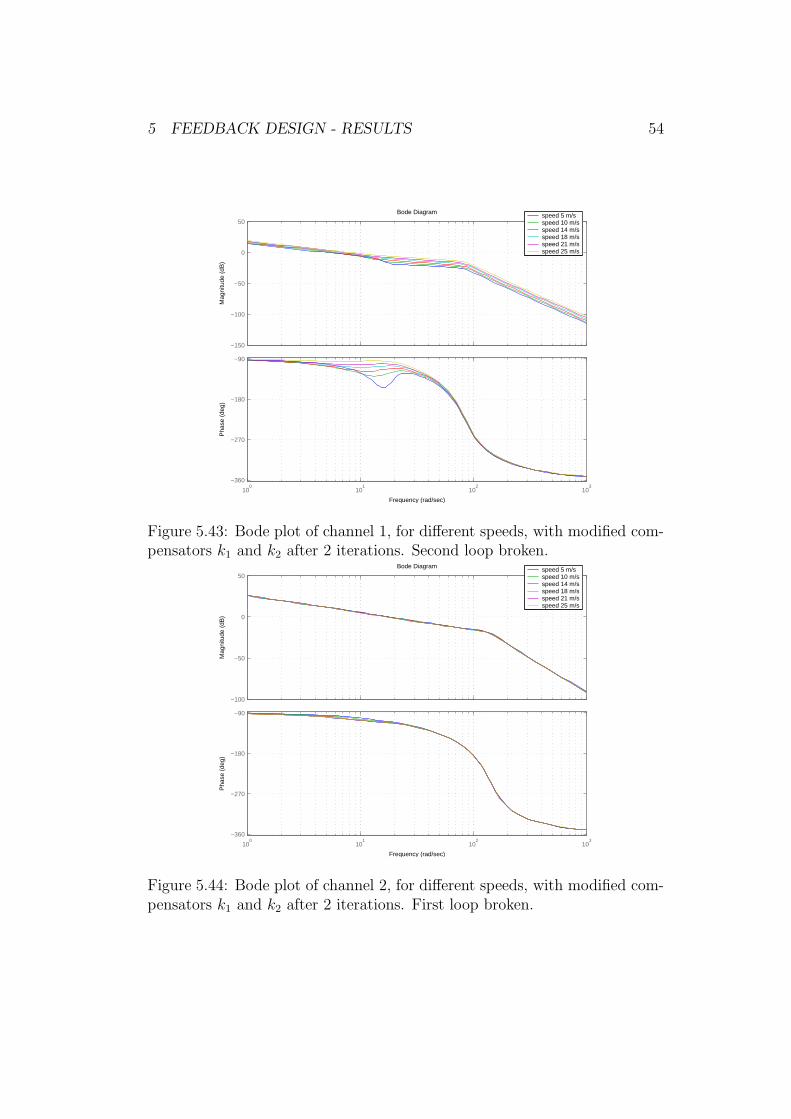
2. The bode plots of k1g11 and k2g22, for speeds between 5 m/s and 25m/s, are shown in figures 5.43 and 5.44. The phase margin is well above−180◦, which proves the stability of h1 and h2.
Similarly, the requirements for robustness from section 4.3 are checked:
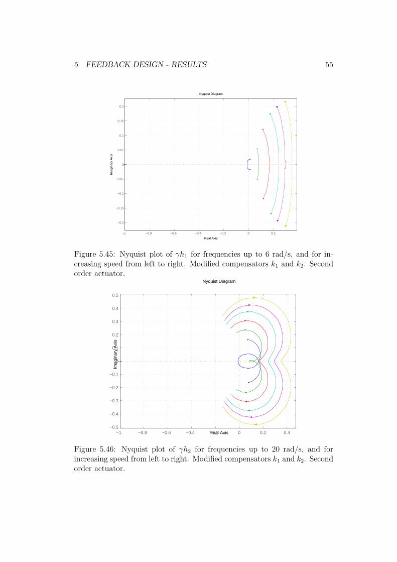
1. The phase margins from table 5.5 do not fall below the specified value.
2. Figures 5.45 and 5.46 show Nyquist plots of γh1 and γh2, for frequenciesup to the crossover frequency. Neither of them goes close to the point(1,0).
5 FEEDBACK DESIGN - RESULTS 54
Bode Diagram
Frequency (rad/sec)
Pha
se (
deg)
Mag
nitu
de (
dB)
−150
−100
−50
0
50speed 5 m/sspeed 10 m/sspeed 14 m/sspeed 18 m/sspeed 21 m/sspeed 25 m/s
100
101
102
103
−360
−270
−180
−90
Figure 5.43: Bode plot of channel 1, for different speeds, with modified com-pensators k1 and k2 after 2 iterations. Second loop broken.
Bode Diagram
Frequency (rad/sec)
Pha
se (
deg)
Mag
nitu
de (
dB)
−100
−50
0
50speed 5 m/sspeed 10 m/sspeed 14 m/sspeed 18 m/sspeed 21 m/sspeed 25 m/s
100
101
102
103
−360
−270
−180
−90
Figure 5.44: Bode plot of channel 2, for different speeds, with modified com-pensators k1 and k2 after 2 iterations. First loop broken.
5 FEEDBACK DESIGN - RESULTS 55
Nyquist Diagram
Real Axis
Imag
inar
y A
xis
−1 −0.8 −0.6 −0.4 −0.2 0 0.2
−0.2
−0.15
−0.1
−0.05
0
0.05
0.1
0.15
0.2
Figure 5.45: Nyquist plot of γh1 for frequencies up to 6 rad/s, and for in-creasing speed from left to right. Modified compensators k1 and k2. Secondorder actuator.
Nyquist Diagram
Real Axis
Imag
inar
y A
xis
−1 −0.8 −0.6 −0.4 −0.2 0 0.2 0.4−0.5
−0.4
−0.3
−0.2
−0.1
0
0.1
0.2
0.3
0.4
0.5
Figure 5.46: Nyquist plot of γh2 for frequencies up to 20 rad/s, and forincreasing speed from left to right. Modified compensators k1 and k2. Secondorder actuator.

6 SIMULATION RESULTS 56
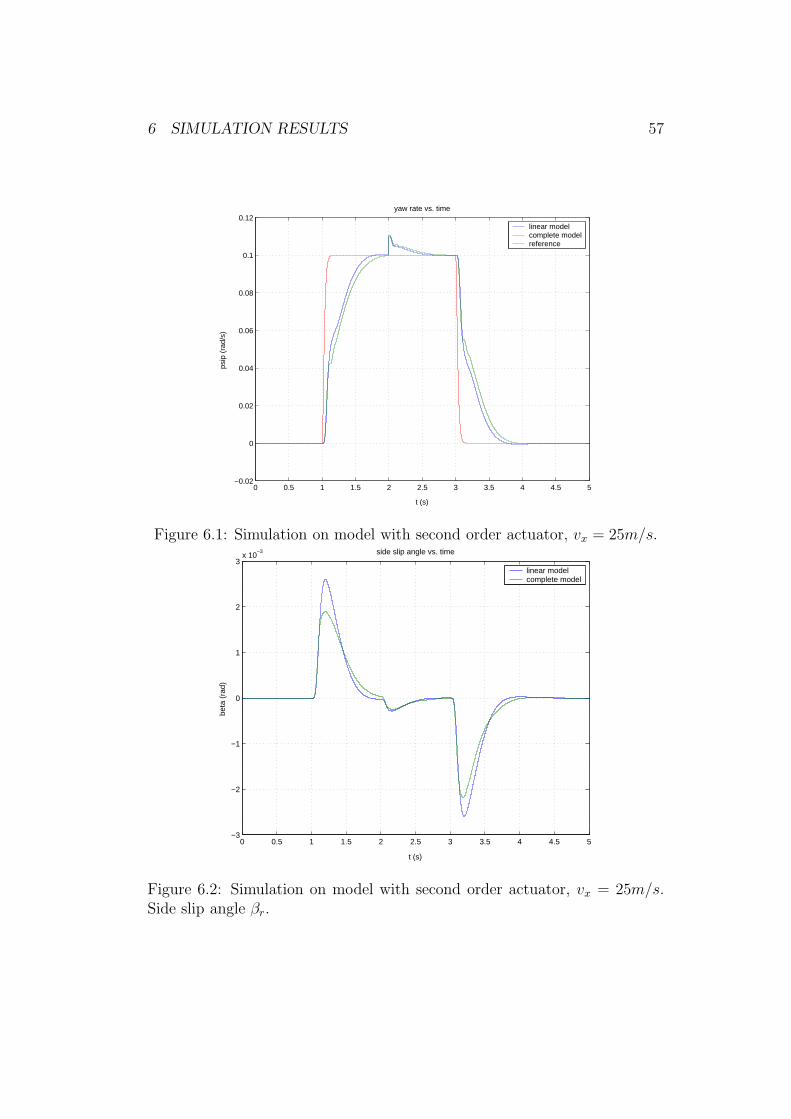
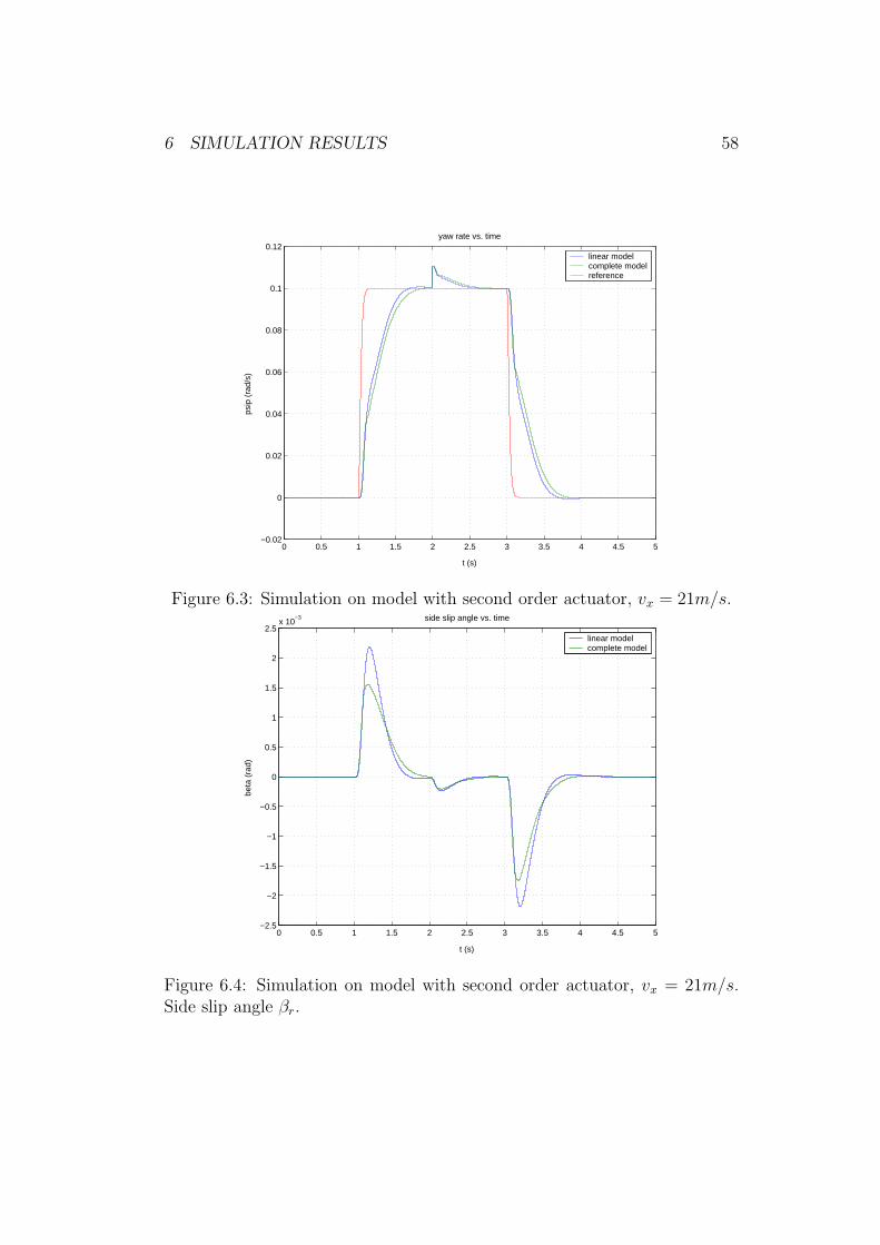
6 Simulation Results
In this section, small signal behaviour of the feedback control will be studied.Simulations are carried out, first on the simple linear one-track model usedfor the design, and later on a nonlinear and more realistic complete 4 wheelsteering vehicle model. Robustness and system integrity of the design will betested by applying a 20 ms time delay and breaking one of the control loops.A small impulse disturbance will be used to check the disturbance rejection.
The model that is used for simulation has 4 wheel steering and all thenonlinear dynamics present in a real vehicle. It is programmed in C, with aninterface to Matlab Simulink. Inputs to the model are front and rear wheelsteering angles, brake torque, surface parameters such as slope and frictioncoefficients, and drive train torque. All outputs are measurable states. Theoutputs are the lateral and longitudinal acceleration, rotational wheel speeds,and the yaw rate. The lateral and longitudinal velocities, needed to calculatethe side slip angle, are observable states and are kept in a logged output. Acontroller for longitudinal speed is needed to prevent the speed from droppingwhile making a turning manoeuvre.
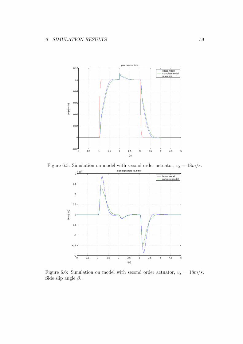
Figures 6.1 to 6.14 show simulations after using the control design andscheduling from chapter 5. A lowpass filtered step reference of 0.1 rad/s(5.7◦/s) for yaw rate, and a small impulse disturbance 1 second after thestep, are used, beyond trying to keep the side slip angle as small as possible(constant reference of 0 radians). From these figures, a decreasing peak ofthe side slip angle, as the speed decreases, can be observed. Beyond that,the observations from section 5.1 are confirmed; for low speeds, on the linearmodel, there it a more oscillatory behaviour. This is not so evident on thecomplete model, probably because of smaller gain or more damping.
6.1 Introducing Time Delay
The control system is designed with enough phase margin to handle a 20ms time delay. But, its robustness has to be proved, and, even with plantuncertainties, it has to behave in a satisfactory manner. This is shown infigures 6.15 to 6.28. In general, the yaw rate step response has slightly moreovershoot than in the case without time delay. Similarly, the peak of theside slip angle is larger than in the previous case. The jagged behaviour thatcan be seen for high speed, in figure 6.15, can be compensated for by thefeedforward. Figures 6.29 and 6.30 show the simulations for speeds between5 and 25 m/s.
6 SIMULATION RESULTS 57
0 0.5 1 1.5 2 2.5 3 3.5 4 4.5 5−0.02
0
0.02
0.04
0.06
0.08
0.1
0.12
t (s)
psip
(ra
d/s)
yaw rate vs. time
linear modelcomplete modelreference
Figure 6.1: Simulation on model with second order actuator, vx = 25m/s.
0 0.5 1 1.5 2 2.5 3 3.5 4 4.5 5−3
−2
−1
0
1
2
3x 10
−3
t (s)
beta
(ra
d)
side slip angle vs. time
linear modelcomplete model
Figure 6.2: Simulation on model with second order actuator, vx = 25m/s.Side slip angle βr.
6 SIMULATION RESULTS 58
0 0.5 1 1.5 2 2.5 3 3.5 4 4.5 5−0.02
0
0.02
0.04
0.06
0.08
0.1
0.12
t (s)
psip
(ra
d/s)
yaw rate vs. time
linear modelcomplete modelreference
Figure 6.3: Simulation on model with second order actuator, vx = 21m/s.
0 0.5 1 1.5 2 2.5 3 3.5 4 4.5 5−2.5
−2
−1.5
−1
−0.5
0
0.5
1
1.5
2
2.5x 10
−3
t (s)
beta
(ra
d)
side slip angle vs. time
linear modelcomplete model
Figure 6.4: Simulation on model with second order actuator, vx = 21m/s.Side slip angle βr.
6 SIMULATION RESULTS 59
0 0.5 1 1.5 2 2.5 3 3.5 4 4.5 5−0.02
0
0.02
0.04
0.06
0.08
0.1
0.12
t (s)
psip
(ra
d/s)
yaw rate vs. time
linear modelcomplete modelreference
Figure 6.5: Simulation on model with second order actuator, vx = 18m/s.
0 0.5 1 1.5 2 2.5 3 3.5 4 4.5 5−2
−1.5
−1
−0.5
0
0.5
1
1.5
2x 10
−3
t (s)
beta
(ra
d)
side slip angle vs. time
linear modelcomplete model
Figure 6.6: Simulation on model with second order actuator, vx = 18m/s.Side slip angle βr.

6 SIMULATION RESULTS 60
0 0.5 1 1.5 2 2.5 3 3.5 4 4.5 5−0.02
0
0.02
0.04
0.06
0.08
0.1
0.12
t (s)
psip
(ra
d/s)
yaw rate vs. time
linear modelcomplete modelreference
Figure 6.7: Simulation on model with second order actuator, vx = 14m/s.
0 0.5 1 1.5 2 2.5 3 3.5 4 4.5 5−1.5
−1
−0.5
0
0.5
1
1.5x 10
−3
t (s)
beta
(ra
d)
side slip angle vs. time
linear modelcomplete model
Figure 6.8: Simulation on model with second order actuator, vx = 14m/s.Side slip angle βr.
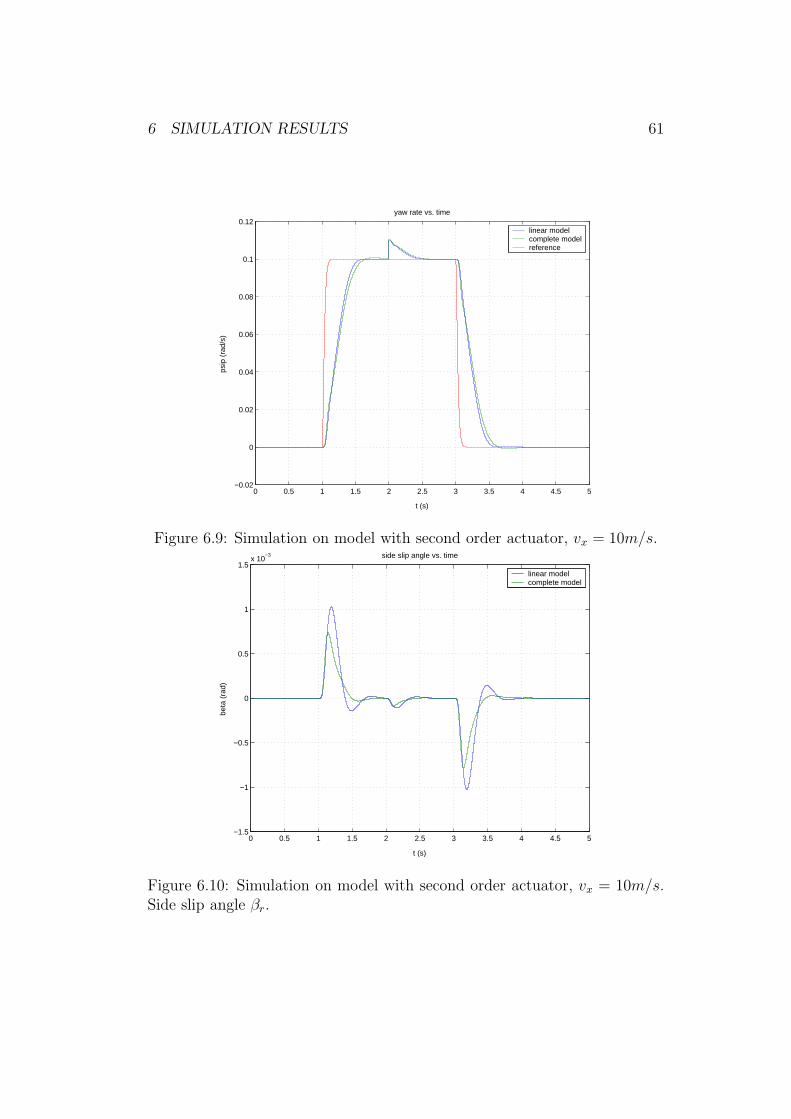
6 SIMULATION RESULTS 61
0 0.5 1 1.5 2 2.5 3 3.5 4 4.5 5−0.02
0
0.02
0.04
0.06
0.08
0.1
0.12
t (s)
psip
(ra
d/s)
yaw rate vs. time
linear modelcomplete modelreference
Figure 6.9: Simulation on model with second order actuator, vx = 10m/s.
0 0.5 1 1.5 2 2.5 3 3.5 4 4.5 5−1.5
−1
−0.5
0
0.5
1
1.5x 10
−3
t (s)
beta
(ra
d)
side slip angle vs. time
linear modelcomplete model
Figure 6.10: Simulation on model with second order actuator, vx = 10m/s.Side slip angle βr.
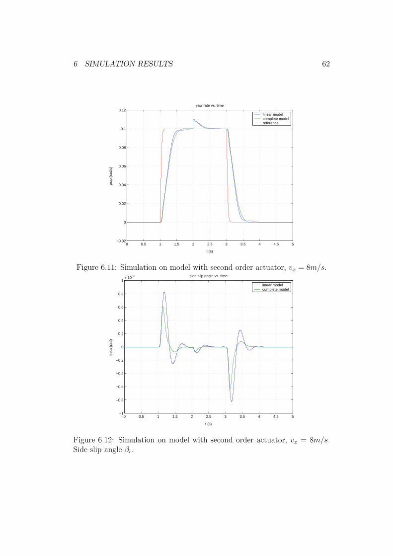
6 SIMULATION RESULTS 62
0 0.5 1 1.5 2 2.5 3 3.5 4 4.5 5−0.02
0
0.02
0.04
0.06
0.08
0.1
0.12
t (s)
psip
(ra
d/s)
yaw rate vs. time
linear modelcomplete modelreference
Figure 6.11: Simulation on model with second order actuator, vx = 8m/s.
0 0.5 1 1.5 2 2.5 3 3.5 4 4.5 5−1
−0.8
−0.6
−0.4
−0.2
0
0.2
0.4
0.6
0.8
1x 10
−3
t (s)
beta
(ra
d)
side slip angle vs. time
linear modelcomplete model
Figure 6.12: Simulation on model with second order actuator, vx = 8m/s.Side slip angle βr.

6 SIMULATION RESULTS 63
0 0.5 1 1.5 2 2.5 3 3.5 4 4.5 5−0.02
0
0.02
0.04
0.06
0.08
0.1
0.12
t (s)
psip
(ra
d/s)
yaw rate vs. time
linear modelcomplete modelreference
Figure 6.13: Simulation on model with second order actuator, vx = 5m/s.
0 0.5 1 1.5 2 2.5 3 3.5 4 4.5 5−8
−6
−4
−2
0
2
4
6
8x 10
−4
t (s)
beta
(ra
d)
side slip angle vs. time
linear modelcomplete model
Figure 6.14: Simulation on model with second order actuator, vx = 5m/s.Side slip angle βr.

6 SIMULATION RESULTS 64
0 0.5 1 1.5 2 2.5 3 3.5 4 4.5 5−0.02
0
0.02
0.04
0.06
0.08
0.1
0.12
t (s)
psip
(ra
d/s)
yaw rate vs. time. 20 ms delay.
linear modelcomplete modelreference
Figure 6.15: Simulation on model with second order actuator, vx = 25m/s.Time delay 20 ms.
0 0.5 1 1.5 2 2.5 3 3.5 4 4.5 5−4
−3
−2
−1
0
1
2
3
4x 10
−3
t (s)
beta
(ra
d)
side slip angle vs. time. 20 ms delay.
linear modelcomplete model
Figure 6.16: Simulation on model with second order actuator, vx = 25m/s.Side slip angle βr. Time delay 20 ms.
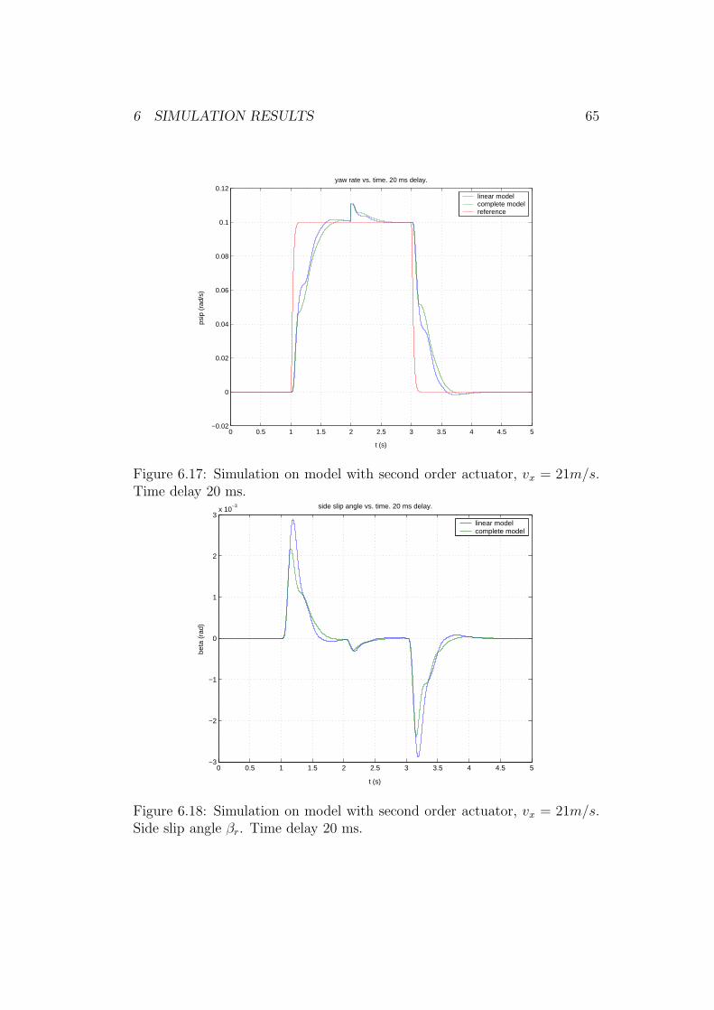
6 SIMULATION RESULTS 65
0 0.5 1 1.5 2 2.5 3 3.5 4 4.5 5−0.02
0
0.02
0.04
0.06
0.08
0.1
0.12
t (s)
psip
(ra
d/s)
yaw rate vs. time. 20 ms delay.
linear modelcomplete modelreference
Figure 6.17: Simulation on model with second order actuator, vx = 21m/s.Time delay 20 ms.
0 0.5 1 1.5 2 2.5 3 3.5 4 4.5 5−3
−2
−1
0
1
2
3x 10
−3
t (s)
beta
(ra
d)
side slip angle vs. time. 20 ms delay.
linear modelcomplete model
Figure 6.18: Simulation on model with second order actuator, vx = 21m/s.Side slip angle βr. Time delay 20 ms.

6 SIMULATION RESULTS 66
0 0.5 1 1.5 2 2.5 3 3.5 4 4.5 5−0.02
0
0.02
0.04
0.06
0.08
0.1
0.12
t (s)
psip
(ra
d/s)
yaw rate vs. time. 20 ms delay.
linear modelcomplete modelreference
Figure 6.19: Simulation on model with second order actuator, vx = 18m/s.Time delay 20 ms.
0 0.5 1 1.5 2 2.5 3 3.5 4 4.5 5−2.5
−2
−1.5
−1
−0.5
0
0.5
1
1.5
2
2.5x 10
−3
t (s)
beta
(ra
d)
side slip angle vs. time. 20 ms delay.
linear modelcomplete model
Figure 6.20: Simulation on model with second order actuator, vx = 18m/s.Side slip angle βr. Time delay 20 ms.

6 SIMULATION RESULTS 67
0 0.5 1 1.5 2 2.5 3 3.5 4 4.5 5−0.02
0
0.02
0.04
0.06
0.08
0.1
0.12
t (s)
psip
(ra
d/s)
yaw rate vs. time. 20 ms delay.
linear modelcomplete modelreference
Figure 6.21: Simulation on model with second order actuator, vx = 14m/s.Time delay 20 ms.
0 0.5 1 1.5 2 2.5 3 3.5 4 4.5 5−2
−1.5
−1
−0.5
0
0.5
1
1.5
2x 10
−3
t (s)
beta
(ra
d)
side slip angle vs. time. 20 ms delay.
linear modelcomplete model
Figure 6.22: Simulation on model with second order actuator, vx = 14m/s.Side slip angle βr. Time delay 20 ms.

6 SIMULATION RESULTS 68
0 0.5 1 1.5 2 2.5 3 3.5 4 4.5 5−0.02
0
0.02
0.04
0.06
0.08
0.1
0.12
t (s)
psip
(ra
d/s)
yaw rate vs. time. 20 ms delay.
linear modelcomplete modelreference
Figure 6.23: Simulation on model with second order actuator, vx = 10m/s.Time delay 20 ms.
0 0.5 1 1.5 2 2.5 3 3.5 4 4.5 5−1.5
−1
−0.5
0
0.5
1
1.5x 10
−3
t (s)
beta
(ra
d)
side slip angle vs. time. 20 ms delay.
linear modelcomplete model
Figure 6.24: Simulation on model with second order actuator, vx = 10m/s.Side slip angle βr. Time delay 20 ms.

6 SIMULATION RESULTS 69
0 0.5 1 1.5 2 2.5 3 3.5 4 4.5 5−0.02
0
0.02
0.04
0.06
0.08
0.1
0.12
t (s)
psip
(ra
d/s)
yaw rate vs. time. 20 ms delay.
linear modelcomplete modelreference
Figure 6.25: Simulation on model with second order actuator, vx = 8m/s.Time delay 20 ms.
0 0.5 1 1.5 2 2.5 3 3.5 4 4.5 5−1.5
−1
−0.5
0
0.5
1
1.5x 10
−3
t (s)
beta
(ra
d)
side slip angle vs. time. 20 ms delay.
linear modelcomplete model
Figure 6.26: Simulation on model with second order actuator, vx = 8m/s.Side slip angle βr. Time delay 20 ms.

6 SIMULATION RESULTS 70
0 0.5 1 1.5 2 2.5 3 3.5 4 4.5 5−0.02
0
0.02
0.04
0.06
0.08
0.1
0.12
t (s)
psip
(ra
d/s)
yaw rate vs. time. 20 ms delay.
linear modelcomplete modelreference
Figure 6.27: Simulation on model with second order actuator, vx = 5m/s.Time delay 20 ms.
0 0.5 1 1.5 2 2.5 3 3.5 4 4.5 5−1
−0.8
−0.6
−0.4
−0.2
0
0.2
0.4
0.6
0.8
1x 10
−3
t (s)
beta
(ra
d)
side slip angle vs. time. 20 ms delay.
linear modelcomplete model
Figure 6.28: Simulation on model with second order actuator, vx = 5m/s.Side slip angle βr. Time delay 20 ms.

6 SIMULATION RESULTS 71
0 0.5 1 1.5 2 2.5 3 3.5 4 4.5 5−0.02
0
0.02
0.04
0.06
0.08
0.1
0.12
t (s)
psip
yaw rate vs. time in simulation on complete model. 20 ms delay.
speed 5 m/sspeed 8 m/sspeed 10 m/sspeed 14 m/sspeed 18 m/sspeed 21 m/sspeed 25 m/sreference
Figure 6.29: Simulation on model with second order actuator, for differentspeeds. Time delay 20 ms.
0 0.5 1 1.5 2 2.5 3 3.5 4 4.5 5−3
−2
−1
0
1
2
3x 10
−3
t (s)
beta
side slip angle vs. time in simulation on complete model. 20 ms delay.
speed 5 m/sspeed 8 m/sspeed 10 m/sspeed 14 m/sspeed 18 m/sspeed 21 m/sspeed 25 m/s
Figure 6.30: Simulation on model with second order actuator, for differentspeeds. Side slip angle βr. Time delay 20 ms.

6 SIMULATION RESULTS 72
6.2 Keeping the Time Delay and Breaking the SecondLoop
When one actuator fails, or, equivalently, when one of the loops is broken,the system should remain stable. Of course, control of both yaw rate andside slip angle, without using additional intervention such as, for example,braking, is then impossible. Figures 6.31 to 6.36 show the yaw rate and sideslip angle when the rear actuator fails. In section 5.2 the performance ofthe controllers under a failure of one of the feedback loops was investigated.Despite a slight loss in phase margin, the performance of the loop in functionremains the same. The side slip angle control remains stable but referencetracking is no longer possible. The steady state error after a couple of secondsis caused by the impulse disturbance applied after 2 seconds, and the absenceof a closed loop integrator.

6 SIMULATION RESULTS 73
0 0.5 1 1.5 2 2.5 3 3.5 4 4.5 5−0.02
0
0.02
0.04
0.06
0.08
0.1
0.12
t (s)
psip
(ra
d/s)
yaw rate vs. time. 20 ms delay. Second loop broken.
linear modelcomplete modelreference
Figure 6.31: Simulation on model with second order actuator, vx = 25m/s.Time delay 20 ms. Second loop broken.
0 0.5 1 1.5 2 2.5 3 3.5 4 4.5 5−2
0
2
4
6
8
10
12x 10
−3
t (s)
beta
(ra
d)
side slip angle vs. time. 20 ms delay. Second loop broken.
linear modelcomplete model
Figure 6.32: Simulation on model with second order actuator, vx = 25m/s.Side slip angle βr. Time delay 20 ms. Second loop broken.

6 SIMULATION RESULTS 74
0 0.5 1 1.5 2 2.5 3 3.5 4 4.5 5−0.02
0
0.02
0.04
0.06
0.08
0.1
0.12
t (s)
psip
(ra
d/s)
yaw rate vs. time. 20 ms delay. Second loop broken.
linear modelcomplete modelreference
Figure 6.33: Simulation on model with second order actuator, vx = 18m/s.Time delay 20 ms. Second loop broken.
0 0.5 1 1.5 2 2.5 3 3.5 4 4.5 5−2
0
2
4
6
8
10x 10
−3
t (s)
beta
(ra
d)
side slip angle vs. time. 20 ms delay. Second loop broken.
linear modelcomplete model
Figure 6.34: Simulation on model with second order actuator, vx = 18m/s.Side slip angle βr. Time delay 20 ms. Second loop broken.

6 SIMULATION RESULTS 75
0 0.5 1 1.5 2 2.5 3 3.5 4 4.5 5−0.02
0
0.02
0.04
0.06
0.08
0.1
0.12
t (s)
psip
(ra
d/s)
yaw rate vs. time. 20 ms delay. Second loop broken.
linear modelcomplete modelreference
Figure 6.35: Simulation on model with second order actuator, vx = 10m/s.Time delay 20 ms. Second loop broken.
0 0.5 1 1.5 2 2.5 3 3.5 4 4.5 5−1
−0.5
0
0.5
1
1.5
2
2.5
3
3.5
4x 10
−3
t (s)
beta
(ra
d)
side slip angle vs. time. 20 ms delay. Second loop broken.
linear modelcomplete model
Figure 6.36: Simulation on model with second order actuator, vx = 10m/s.Side slip angle βr. Time delay 20 ms. Second loop broken.

7 CONCLUSIONS AND FUTURE WORK 76
7 Conclusions and Future Work
The main concept of this work has been the design of a diagonal feedbackcontroller for yaw rate and side slip angle, using front and rear wheel steer-ing. With the today existing decoupled design, there are obvious difficultiesin obtaining a robust solution that can handle time delays as well as actu-ator and sensor failures or constraint hitting. Instead, coupling based onIndividual Channel Design has been applied.
Of all approaches tested, the one presented in this report shows the bestability of fulfilling the specifications. It has a rather easy structure and thescheduling is quite straightforward. It can also easily be implemented as aPID-controller.
System integrity, or the performance of the closed-loop system under afailure of one of the feedback loops, has been studied. The theoretical re-quirements have been tested, by studying the pole placement of the channels,and by simulating on a car model.
Robustness to plant uncertainty is very important for the controller towork on a real plant. It can to some extent be verified in theory. Thishas been done by studying the structure function of the system, and bysimulating on the car model. A 20 ms time delay has also been used tocheck the robustness. During the design it has been noticed that the plantdynamics show great variations with changing tyre characteristics, such as,for instance, the stiffness. This further increases the importance of having arobust solution.
The physical environment is very uncertain. Changes in the road surfaceand wind disturbances are always present. A rejection of those disturbancesis important. An integrator is used in the controller to avoid steady stateerrors.
The specified bandwidth and phase margin have been obtained with thefeedback design for the second channel. The first channel turned out to bequite ill behaved, and the bandwidth specification had to be relaxed for thefirst feedback loop. The lower bandwidth used will affect the performancein terms of the step and impulse response rise time. Despite the slowercharacteristics of the first loop, and the fact that the original specificationscould not be completely fulfilled, feedback can still be used for both frontand rear wheel steering.
A feedforward still remains to be designed. This can be done by usingthe general ideas about feedforward (some are presented in section 3.2). Thefeedforward used with the today existing feedback design, can possibly beapplied. Furthermore, it should be investigated whether a change of theoutputs would make design somewhat easier. The controllers also need to beimplemented, and finally tested in the experimental vehicle.
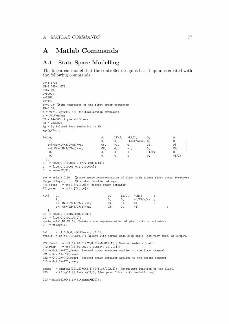
A MATLAB COMMANDS 77
A Matlab Commands
A.1 State Space Modelling
The linear car model that the controller design is based upon, is created withthe following commands:
LV=1.673;
LH=3.085-1.673;
L=LV+LH;
J=5000;
m=2364;
vx=14;
TV=0.03; %time constants of the first order actuators
TH=0.03;
a = vx/(0.03*vx+0.5); %initialisation transient
b = J/LV/m/vx;
CV = 144000; %tyre stiffness
CH = 283000;
fg = 3; %closed loop bandwidth in Hz
wg=fg*2*pi;
A=[ 0, 0, LV/J, -LH/J, 0, 0 ;
1, 0, 0, -L/LV/m/vx, 0, 0 ;
a*[-CV*(LV+J/LV/m)/vx, CV, -1, 0, CV, 0] ;
a*[ CH*(LH-J/LV/m)/vx, CH, 0, -1, 0, CH] ;
0, 0, 0, 0, -1/TV, 0 ;
0, 0, 0, 0, 0, -1/TH ;
];
B = [0,0;0,0;0,0;0,0;1/TV,0;0,1/TH];
C = [1,0,0,0,0,0; 0,1,0,0,0,0];
D = zeros(2,2);
sys = ss(A,B,C,D); %state space representation of plant with linear first order actuators.
Gbig= tf(sys); %transfer function of sys.
PT1_front = tf(1,[TV,1,0]); %first order actuator
PT1_rear = tf(1,[TH,1,0]);
A1=[ 0, 0, LV/J, -LH/J ;
1, 0, 0, -L/LV/m/vx ;
a*[-CV*(LV+J/LV/m)/vx, CV, -1, 0] ;
a*[ CH*(LH-J/LV/m)/vx, CH, 0, -1] ;
];
B1 = [0,0;0,0;a*CV,0;0,a*CH];
C1 = [1,0,0,0;0,1,0,0];
sys1= ss(A1,B1,C1,D); %state space representation of plant with no actuators.
G = tf(sys1);
Calt = [1,0,0,0;-J/LV/m/vx,1,0,0];
sysalt = ss(A1,B1,Calt,D); %plant with normal side slip angle (not rear axle) as output.
PT2_front = tf([1],[0.012^2,0.612*0.012,1]); %second order actuator
PT2_rear = tf([1],[0.0072^2,0.612*0.0072,1]);
G11 = G(1,1)*PT2_front; %second order actuator applied to the first channel.
G21 = G(2,1)*PT2_front;
G22 = G(2,2)*PT2_rear; %second order actuator applied to the second channel.
G12 = G(1,2)*PT2_rear;
gamma = minreal(G(1,2)*G(2,1)/G(1,1)/G(2,2)); %structure function of the plant.
H20 = tf(wg^2,[1,2*wg,wg^2]); %low pass filter with bandwidth wg.
G10 = minreal(G(1,1)*(1-gamma*H20));
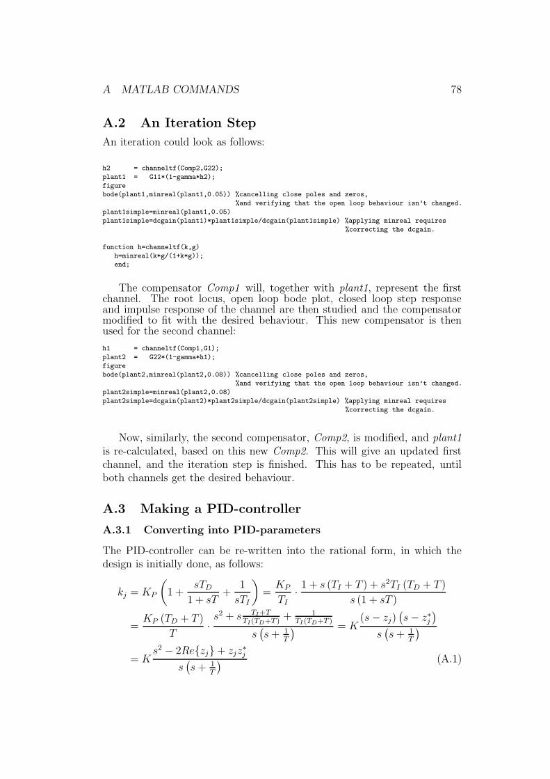
A MATLAB COMMANDS 78
A.2 An Iteration Step
An iteration could look as follows:
h2 = channeltf(Comp2,G22);
plant1 = G11*(1-gamma*h2);
figure
bode(plant1,minreal(plant1,0.05)) %cancelling close poles and zeros,
%and verifying that the open loop behaviour isn’t changed.
plant1simple=minreal(plant1,0.05)
plant1simple=dcgain(plant1)*plant1simple/dcgain(plant1simple) %applying minreal requires
%correcting the dcgain.
function h=channeltf(k,g)
h=minreal(k*g/(1+k*g));
end;
The compensator Comp1 will, together with plant1, represent the firstchannel. The root locus, open loop bode plot, closed loop step responseand impulse response of the channel are then studied and the compensatormodified to fit with the desired behaviour. This new compensator is thenused for the second channel:
h1 = channeltf(Comp1,G1);
plant2 = G22*(1-gamma*h1);
figure
bode(plant2,minreal(plant2,0.08)) %cancelling close poles and zeros,
%and verifying that the open loop behaviour isn’t changed.
plant2simple=minreal(plant2,0.08)
plant2simple=dcgain(plant2)*plant2simple/dcgain(plant2simple) %applying minreal requires
%correcting the dcgain.
Now, similarly, the second compensator, Comp2, is modified, and plant1is re-calculated, based on this new Comp2. This will give an updated firstchannel, and the iteration step is finished. This has to be repeated, untilboth channels get the desired behaviour.
A.3 Making a PID-controller
A.3.1 Converting into PID-parameters
The PID-controller can be re-written into the rational form, in which thedesign is initially done, as follows:
kj = KP
(
1 +sTD
1 + sT+
1
sTI
)
=KP
TI·1 + s (TI + T ) + s2TI (TD + T )
s (1 + sT )
=KP (TD + T )
T·s2 + s TI+T
TI(TD+T )+ 1
TI (TD+T )
s(
s+ 1T
) = K(s− zj)
(
s− z∗j)
s(
s+ 1T
)
= Ks2 − 2Re{zj} + zjz
∗
j
s(
s + 1T
) (A.1)

A MATLAB COMMANDS 79
This would give the PID-parameters in terms of T , the complex zero pair zj
and z∗j , and gain K:
TI = −2Re{zj}
zjz∗j− T (A.2)
TD =1
TI
·1
zjz∗
j
− T (A.3)
KP = KT
TD + T(A.4)
A.3.2 Scheduling with respect to speed
The controller zero is placed right on the lightly damped pole of the plant.The complex zero calculation is done with the following function, where theinputs are the car parameters and the current speed.
function z=makezero(LV,LH,m,J,CV,CH,vx)
L=LV+LH; a = vx/(0.03*vx+0.5);
pss_f=-CV*(LV+J/(LV*m))/vx;
pss_r=CH*(LH-J/(LV*m))/vx;
A1pol=[ 1;
2*a;
a^2+a*CH*L/(LV*m*vx)-(a*pss_f*LV/J)+a*pss_r*LH/J;
a^2*CH*L/(LV*m*vx)-(a*CV*LV/J)-(a^2*pss_f*LV/J)+a^2*pss_r*LH/J+a*CH*LH/J;
-a^2*CV*LV/J-a^2*CH*pss_f*L/(LV*m*vx)*LV/J+a^2*CV*pss_r*L/(LV*m*vx)*LV/J+a^2*CH*LH/J
]’; %characteristic polynomial of the state matrix A.
poles=roots(A1pol); %poles of the plant.
place_of_pole=find(real(poles)==max(real(poles))); %finds the lightly damped pole.
z=poles(place_of_pole(1));
z=real(z)+abs(imag(z))*i; %returns the lightly damped pole with positive imaginary part.
The compensator gains, K1 and K2, are calculated as follows:
function [Gain_Comp1,GainComp2] = makegain(LV,LH,m,J,CV,CH,vx)
L=LV+LH;
a = vx/(0.03*vx+0.5);
A1=[ 0, 0, LV/J, -LH/J;
1, 0, 0, -L/LV/m/vx;
a*[-CV*(LV+J/LV/m)/vx, CV, -1, 0];
a*[ CH*(LH-J/LV/m)/vx, CH, 0, -1];
];
B1 = [0,0;0,0;a*CV,0;0,a*CH];
C1 = [1,0,0,0;0,1,0,0];
D = zeros(2,2);
sys1 = ss(A1,B1,C1,D);
G = tf(sys1); %system transfer function
G11 = G(1,1)*tf([1],[0.012^2,0.612*0.012,1]); %second order actuator applied to channel 1.
G22 = G(2,2)*tf([1],[0.0072^2,0.612*0.0072,1]); %second order actuator applied to channel 2.
gamma = minreal(G(1,2)*G(2,1)/G(1,1)/G(2,2));
zero = makezero(LV,LH,m,J,CV,CH,vx); %finds the complex zero for speed vx.
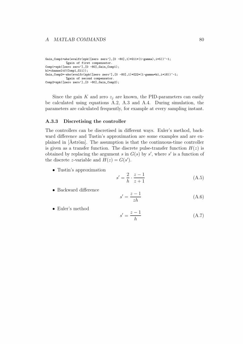
A MATLAB COMMANDS 80
Gain_Comp1=abs(evalfr(zpk([zero zero’],[0 -80],1)*G11*(1-gamma),i*5))^-1;
%gain of first compensator.
Comp1=zpk([zero zero’],[0 -80],Gain_Comp1);
h1=channeltf(Comp1,G11));
Gain_Comp2=-abs(evalfr(zpk([zero zero’],[0 -80],1)*G22*(1-gamma*h1,i*18))^-1;
%gain of second compensator.
Comp2=zpk([zero zero’],[0 -80],Gain_Comp2);
Since the gain K and zero zj are known, the PID-parameters can easilybe calculated using equations A.2, A.3 and A.4. During simulation, theparameters are calculated frequently, for example at every sampling instant.
A.3.3 Discretising the controller
The controllers can be discretised in different ways. Euler’s method, back-ward difference and Tustin’s approximation are some examples and are ex-plained in [Astrom]. The assumption is that the continuous-time controlleris given as a transfer function. The discrete pulse-transfer function H(z) isobtained by replacing the argument s in G(s) by s′, where s′ is a function ofthe discrete z-variable and H(z) = G(s′).
• Tustin’s approximation
s′ =2
h·z − 1
z + 1(A.5)
• Backward difference
s′ =z − 1
zh(A.6)
• Euler’s method
s′ =z − 1
h(A.7)

REFERENCES 81
References
[Glad] Torkel Glad, Lennart Ljung, Reglerteknik, Grundlaggandeteori, 1997 Studentlitteratur
[Glad2] Torkel Glad, Lennart Ljung, Reglerteori, Flervariabla ocholinjara metoder, 1997 Studentlitteratur
[Hayes] Monson H. Hayes, Statistical Digital Signal Processing andModeling, John Wiley & Sons 1996
[Horowitz] Isaac M. Horowitz, Synthesis of Feedback Systems, AcademicPress 1963
[Kalkkuhl] Jens Kalkkuhl, Individual Channel Design - Ein Werkzeugzur Analyse und Synthese Robuster Mehrgrossenregelungenim Frequenzbereich, Daimler Benz 1997
[Kiencke] U. Kiencke, L. Nielsen, Automotive Control Systems, For En-gine, Driveline, and Vehicle, 2000 Springer
[Kleinschrodt] Thomas Kleinschrodt, Four Wheel Steering Considering theNonlinear Wheel Slip - An Anti Windup Problem, DaimlerChrysler 2001
[Leithead,O’Reilly] W.E. Leithead,J. O’Reilly, Performance issues in the in-dividual channel design of 2-input 2-output systems, Int. J.Control 1991-1992
[Maciejowski] J.M. Maciejowski, Multivariable Feedback Design, 1989Addison-Wesley
[Niethammer] Marc Niethammer, Reglerentwurf fur ein Fahrzeug mitlenkbarer Vorder- und Hinterachse, Daimler Chrysler 2000
[Nieuwstadt] Michiel J. van Nieuwstadt, Trajectory Generation for Nonlin-ear Control Systems, California Institute of Technology 1997
[Arzen] Karl-Erik Arzen, Real-Time Control Systems, Dept. of Auto-matic Control, Lund Institute of Technology 2001
[Astrom] K.J. Astrom, Bjorn Wittenmark, Computer Controlled Sys-tems, Theory and Design, 3rd ed, 1997 Prentice Hall


![Enabling Testing of Lateral Active Safety Functions in a ...Notation Notations Bicycle Model Notation Meaning z Yaw angle [deg] z Yaw rate [deg/s] f Steering angle [deg] m Vehicle](https://img.pdfslide.us/doc/110x75/5f2a0d0f0b144d4639358dc0/enabling-testing-of-lateral-active-safety-functions-in-a-notation-notations.jpg)