Embed Size (px)
Citation preview

Optimal Shape Design for Open Rotor Blades
Thomas D. Economon
⇤, Francisco Palacios
†, and Juan J. Alonso
‡,
Stanford University, Stanford, CA 94305, U.S.A.
A continuous adjoint formulation for optimal shape design of rotating surfaces, includingopen rotor blades, is developed, analyzed, and applied. The compressible Euler equationsare expressed in a rotating reference frame, and from these governing flow equations, anadjoint formulation centered around finding surface sensitivities using di↵erential geom-etry is derived. The surface formulation provides the gradient information necessary forperforming gradient-based aerodynamic shape optimization. A two-dimensional test caseconsisting of a rotating airfoil is used to verify the accuracy of the gradient informationobtained via the adjoint method against finite di↵erencing, and a gradient accuracy studyis also performed. The shape of the airfoil is then optimized for drag minimization in thepresence of transonic shocks. In three-dimensions, the formulation is verified against finitedi↵erencing for a classic, two-bladed rotor, which is then redesigned for minimum inviscidtorque using a Free-Form Deformation approach to geometry parameterization. Optimalshape design for open rotor blades is presented as a final application of the new continuousadjoint formulation.
Nomenclature
V ariable Definition
c Airfoil chord length~d Force projection vectorjS
Scalar function defined at each point on S~n Unit normal vectorp Static pressurep1 Freestream pressure~r Position vector from the frame rotation center to a point in the flow domain~r
o
Specified frame rotation center~u
r
Velocity due to rotation at a point, ~! ⇥ ~r~v Flow velocity vector in the intertial frame~v
r
Relative flow velocity vector, ~v � ~ur
v1 Freestream velocity~A Euler flux Jacobian matricesA
z
Projected area in the z-directionC
d
Coe�cient of dragC
l
Coe�cient of liftC
p
Coe�cient of pressureC
Q
Coe�cient of torque, Q/(0.5⇢1⇡R3(!R)2)C
T
Coe�cient of thrust, T/(0.5⇢1⇡R2(!R)2 )E Total energy per unit mass~F Euler convective fluxes~F
rot
Rotating Euler convective fluxesH Stagnation enthalpy
⇤Ph.D. Candidate, Department of Aeronautics & Astronautics, AIAA Student Member.†Engineering Research Associate, Department of Aeronautics & Astronautics, AIAA Member.‡Associate Professor, Department of Aeronautics & Astronautics, AIAA Senior Member.
1 of 23
American Institute of Aeronautics and Astronautics
30th AIAA Applied Aerodynamics Conference25 - 28 June 2012, New Orleans, Louisiana
AIAA 2012-3018
Copyright © 2012 by the authors. Published by the American Institute of Aeronautics and Astronautics, Inc., with permission.
Dow
nloa
ded
by S
tanf
ord
Uni
vers
ity o
n Se
ptem
ber
27, 2
012
| http
://ar
c.ai
aa.o
rg |
DO
I: 1
0.25
14/6
.201
2-30
18

Hm
Mean curvature of a surface¯I Identity matrixJ Cost function defined as an integral over SM1 Freestream Mach numberQ Rotor torqueQ Vector of source termsR Rotor radiusR(U) System of governing flow equationsS Solid wall domain boundary (design surface)T Rotor thrustT Rotation matrix for transforming data between periodic boundariesU Vector of conservative variablesW Vector of characteristic variables↵ Angle of attack� Sideslip angle� Ratio of specific heats, � = 1.4 for air⇢ Fluid density⇢1 Freestream density~� Adjoint velocity vector~! Specified angular velocity vector of the rotating frame! Angular velocity magnitude� Far-field domain boundary Vector of adjoint variables⌦ Flow domain
Mathematical Notation
~b Spatial vector b 2 Rn, where n is the dimension of the physical cartesian space (in general, 2 or 3)B Column vector or matrix B, unless capitalized symbol clearly defined otherwise~B ~B = (B
x
, By
) in two dimensions or ~B = (Bx
, By
, Bz
) in three dimensionsr(·) Gradient operatorr · (·) Divergence operator@
n
(·) Normal gradient operator at a surface point, ~nS
·r(·)r
S
(·) Tangential gradient operator at a surface point, r(·) � @n
(·)· Vector inner product⇥ Vector cross product⌦ Vector outer productBT Transpose operation on column vector or matrix B�(·) Denotes first variation of a quantity
I. Introduction and Motivation
Environmental pressures to decrease both fuel burn and emissions, coupled with fuel price volatility,continue to drive the need for more e�cient aircraft propulsion technology. Open rotor propulsion systems
have long been studied due to their potential for game-changing advances in propulsive e�ciency. Previousflight testing by General Electric, Pratt & Whitney, and NASA [1] has shown that open rotor engines loweredspecific fuel consumption for an MD-80 and a B727 between 20-40 % depending on the type of engine beingreplaced and the choice of flight cruise Mach number. Furthermore, this fuel burn reduction was consideredconservative, as it was based on a demonstrator engine alone, and not a finalized, production engine. Otherwork has estimated that open rotors could save approximately 30 % of the fuel cost for a medium rangetransport, and about 12 % of the total direct operating cost of the aircraft [2]. These results were based ondated fuel prices which were lower than current values, and emphasis should be placed on the likelihood offuel price volatility continuing in the future.
Although the technology is promising, significant challenges must be addressed before a wide-spreadadoption of open rotors occurs: assessing possible increases in noise, the potential aircraft structural weightpenalties of noise insulation or protection from blade-out, and potential weight and/or cost penalties of
2 of 23
American Institute of Aeronautics and Astronautics
Dow
nloa
ded
by S
tanf
ord
Uni
vers
ity o
n Se
ptem
ber
27, 2
012
| http
://ar
c.ai
aa.o
rg |
DO
I: 1
0.25
14/6
.201
2-30
18

the open rotors as compared to turbofans [3]. These same challenges also o↵er an opportunity for theaircraft designer to take advantage of synergistic interactions between the configuration design and openrotor installation. New proposals for unconventional aircraft configurations or engine placement may targetenhanced aerodynamic performance, noise shielding, or provide safety in the event of blade-out. Thesecomplex systems will require high fidelity analysis and system-level integration studies in order to assess theviability of the open rotor as a next generation propulsion system. Interaction e↵ects during installation andthe potential for large increases in noise have recently garnered much interest in the research community [4–8].
As a first step toward the multidisciplinary design of open rotors, this paper describes a new adjoint-based methodology to be used for the e�cient optimal shape design of rotating aerodynamic surfaces, such asrotor blades. By focusing on an axisymmetric, single rotor configuration, the governing Euler flow equationscan be recast into a rotating frame of reference moving with the body, and this transformation allows forthe steady solution of a problem which was unsteady in the inertial frame. Adjoint-based formulations foroptimal shape design of steady problems have a rich history in aeronautics, and their e↵ectiveness is wellestablished [9–11].
Rotor design has long been pursued using various techniques, but to our knowledge, only several pub-lications have addressed adjoint-based shape design using the non-inertial governing flow equations. Leeand Kwon [12] presented a continuous adjoint formulation for inviscid, hovering rotor flows on unstructuredmeshes. More recently, discrete adjoint formulations for the Reynolds-averaged Navier-Stokes (RANS) equa-tions in a rotating frame have been shown by Nielsen et al. [13] with the Spalart-Allmaras turbulence modelon unstructured meshes and by Dumont et al. [14] with the k � ! turbulence model and the shear stresstransport correction on structured meshes.
⌦�1
S~n
S
~n�1
�1
�p1 �
p2
~n�p1 ~n�p2
Figure 1. Notional schematic of the flow do-main, ⌦, and the disconnected boundarieswith their corresponding surface normals: S,�1, as well as new periodic boundaries, �p.
While a discrete adjoint approach can often be morestraightforward to implement, especially if automatic di↵er-entiation is available, we pursue in this article a continuousapproach. The continuous formulation can o↵er the advan-tage of physical insight into the character of the governing flowequations and their adjoint system, and this insight can aidin composing well-behaved numerical solution methods. Morespecifically, the treatment given in this article is a system-atic methodology for the compressible Euler equations centeredaround finding surface sensitivities with the use of di↵erentialgeometry formulas. The surface sensitivities show the designerexactly where shape changes will have the most e↵ect on a cho-sen objective function. This type of surface formulation has nodependence on volume mesh sensitivities and has been success-fully applied to full aircraft configurations and even extendedto the RANS equations [15, 16]. It is here extended for theoptimal shape design of steadily rotating surfaces. Note thatthis methodology is general and could be used for the design ofother rotating bodies such as propellers, turbomachinery, windturbines, etc.
As there are few applications of these techniques and existing examples have been applied mostly withinthe rotorcraft research community, a novel application to optimal shape design of open rotor blades ispresented. A Free-Form Deformation (FFD) approach to geometry parameterization allows for advanceddesign variable definitions during shape optimization. The combination of the adjoint formulation, unstruc-tured meshes, and the FFD approach give the designer more freedom to explore non-intuitive design spacesinvolving complex geometries such as highly twisted, swept open rotor blades.
The contributions of this article are the following: a detailed derivation of the continuous adjoint for-mulation emphasizing surface sensitivities, practical numerical implementation details for central schemesincluding a new type of dissipation switch, two- and three-dimensional gradient verification for the adjointagainst finite di↵erencing, a gradient accuracy study, and three optimal shape design examples includingopen rotor blades.
The paper begins with a description of the physical problem in Section II, including the governingflow equations with corresponding boundary conditions. Section III contains a detailed derivation of thecontinuous adjoint formulation for the compressible Euler equations in a rotating reference frame. This
3 of 23
American Institute of Aeronautics and Astronautics
Dow
nloa
ded
by S
tanf
ord
Uni
vers
ity o
n Se
ptem
ber
27, 2
012
| http
://ar
c.ai
aa.o
rg |
DO
I: 1
0.25
14/6
.201
2-30
18
derivation is generalized to two or three dimensions. Numerical implementation strategies such as numericalmethods, design variable definition, and mesh deformation appear in Section IV. Lastly, Section V presentsnumerical results and discussion for both two- and three-dimensional numerical experiments, including afinal example for the optimal shape design of open rotor blades.
II. Description of the Physical Problem
Ideal fluids are governed by the Euler equations. In our particular problem, these equations are consideredin a domain, ⌦, bounded by a disconnected boundary which is divided into a far-field component, �1, asolid wall boundary, S, and periodic boundary faces, �
p
, as seen in Fig. 1. The surface S will also bereferred to as the design surface, and it is considered continuously di↵erentiable (C1). In practical shapedesign applications, the assumption of di↵erentiability does not hold for sharp corners or edges that mightappear along trailing edges or the tips of wings or rotor blades. Special considerations must be made at theselocations during the design process, and these will be discussed later with other numerical implementationdetails. Normal vectors to the boundary surfaces are directed out of the domain by convention.
The governing flow equations in the limit of vanishing viscosity are the compressible Euler equations.When simulating fluid flow about certain aerodynamic bodies that operate under an imposed steady rotation,including many turbomachinery, propeller, and rotor applications, it can be advantageous to transformthe system of Euler equations into a reference frame that rotates with the body of interest. With thistransformation, a flow field that is unsteady when viewed from the inertial frame can be solved for in asteady manner, and thus more e�ciently, without the need for grid motion. For conciseness, this formulationof the governing system will be referred to as the rotating Euler equations.
Considering the flow domain of Fig. 1 after performing the appropriate transformation into a referenceframe that rotates with a steady angular velocity, ~! = {!
x
,!y
,!z
}T , and a specified rotation center, ~ro
={x
o
, yo
, zo
}T , the absolute velocity formulation [17] of the steady, rotating Euler equations in conservationform is
8
>
>
>
>
>
<
>
>
>
>
>
:
R(U) = r · ~Frot
�Q = 0 in ⌦,
(~v � ~ur
) · ~nS
= 0 on S,
W+ = W1 on �1,
U1 = T U2 on �p1 ,
U2 = T �1U1 on �p2 ,
(1)
where
U =
8
>
<
>
:
⇢
⇢~v
⇢E
9
>
=
>
;
, ~Frot
=
8
>
<
>
:
⇢(~v � ~ur
)
⇢~v ⌦ (~v � ~ur
) + ¯Ip
⇢H(~v � ~ur
) + ~ur
p
9
>
=
>
;
, Q =
8
>
<
>
:
0
�⇢(~! ⇥ ~v)
0
9
>
=
>
;
,
where ⇢ is the fluid density, ~v = {u, v, w}T is the absolute flow velocity, E is the total energy per unitmass, H is the total enthalpy per unit mass, p is the static pressure, and ~u
r
is the velocity due to rotation(~u
r
= ~! ⇥ ~r). Here, ~r is the position vector pointing from the rotation center to a point (x, y, z) in theflow domain, or ~r = {(x � x
o
), (y � yo
), (z � zo
)}T . The velocity due to rotation is also sometimes calledthe whirl velocity. The second and third lines of Eq. 1 represent the solid wall and characteristic-basedfar-field boundary conditions, respectively, with an adjustment for rotation. Rotor simulations often takeadvantage of rotational periodicity by solving for the flow around a single blade with periodic boundariesrather than the entire set of blades, and this can decrease computational cost greatly. With rotationalperiodicity (fourth and fifth lines of Eq. 1), vector flow quantities at each point, such as the momentum,must be rotated using a transformation matrix, T , so that the angle of incidence between the vector and thedomain boundary remains the same when transforming the state to the corresponding periodic face. Thetransformation matrix, T , can be found in the appendix. In order to close the system of equations afterassuming a perfect gas, the pressure is determined from
p = (� � 1)⇢
E � 1
2(~v · ~v)
�
, (2)
4 of 23
American Institute of Aeronautics and Astronautics
Dow
nloa
ded
by S
tanf
ord
Uni
vers
ity o
n Se
ptem
ber
27, 2
012
| http
://ar
c.ai
aa.o
rg |
DO
I: 1
0.25
14/6
.201
2-30
18

and the stagnation enthalpy is given by
H = E +p
⇢. (3)
It is important to note that not all simulations of rotating bodies can benefit from this solution approach.The flow field must be steady in the rotating frame, and some conditions or geometric features, such as relativesurface motion, can cause unsteadiness for rotating bodies. If the incoming flow velocity is not parallel tothe axis of rotation, the conditions are no longer axisymmetric, and the blades would not see a steady fieldduring rotation. In this case, the rotating Euler equations would not provide an e�cient, steady solutionmethod.
III. Surface Sensitivities Using a Continuous Adjoint Methodology
The objective of this section is to describe the way in which we quantify the influence of geometricmodifications on the pressure distribution at a solid surface in the flow domain. Again, the motivation forpursuing a continuous formulation based on surface sensitivities includes the following important considera-tions: manipulation of the continuous equations o↵ers direct insight into the mathematical character of thegoverning equations, there is no dependence on volume mesh sensitivities when computing the first variationof a functional (only a surface integral remains), and the e↵ect of local surface shape modifications can bedirectly visualized using the surface sensitivities to further designer intuition. It is here that the continuousadjoint formulation is systematically derived following a procedure similar to that of Bueno-Orovio et al. [15].
A typical shape optimization problem seeks the minimization of a certain cost function, J , with respectto changes in the shape of the boundary, S. For example, for the designer concerned with aerodynamicperformance, an obvious choice for J might be the coe�cient of drag on S. Therefore, we will concentrateon functionals defined as integrals over the solid surface S,
J =
Z
S
jS
ds, (4)
where jS
is a scalar function defined at each point on S. As the designer choosing the shape of S, thequestion we would like to answer is the following: what e↵ect does a change in the shape of S have on thevalue of J? In the case of drag minimization mentioned above, shape deformations that reduce the drag onthe surface are desired.
�S~nS
S
S0
~x
Figure 2. An infinitesimal shape deformation inthe local surface normal direction.
Therefore, the goal is to compute the variation of Eq. 4caused by arbitrary but small (and multiple) deformationsof S and to use this information to drive our geometricchanges in order to find an optimal shape for the designsurface, S. This leads directly to a gradient-based op-timization framework. The shape deformations appliedto S will be infinitesimal in nature and can be describedmathematically by
S0 = {~x + �S(~x)~nS
(~x), ~x 2 S}, (5)
where S has been deformed to a new surface S0 by apply-ing an infinitesimal profile deformation, �S, in the local normal direction, ~n
S
, at a point, ~x, on the surface,as shown in Fig. 2. Upon application of the surface deformation, the cost function varies due to the changesin the solution induced by the deformation:
�J =
Z
�S
jS
ds +
Z
S
�jS
ds. (6)
Note that taking the variation results in two separate terms. The first term depends on the variation of thegeometry and the value of the scalar function in the original state, while the second term depends on theoriginal geometry and the variation of the scalar function caused by the deformation.
With the basic outline of the shape design problem described, let us more specifically define the scalarfunction as
jS
= ~d · (p~nS
). (7)
5 of 23
American Institute of Aeronautics and Astronautics
Dow
nloa
ded
by S
tanf
ord
Uni
vers
ity o
n Se
ptem
ber
27, 2
012
| http
://ar
c.ai
aa.o
rg |
DO
I: 1
0.25
14/6
.201
2-30
18

The vector ~d is the force projection vector, and it is an arbitrary, constant vector which can be chosen torelate the pressure, p, at the surface to a desired quantity of interest. For aerodynamic applications, likelycandidates are
~d =
8
>
>
>
>
>
>
>
>
>
>
>
>
<
>
>
>
>
>
>
>
>
>
>
>
>
:
⇣
1C1
⌘
(cos ↵ cos �, sin ↵ cos �, sin �), CD
Drag coe�cient,⇣
1C1
⌘
(� sin ↵, cos ↵, 0), CL
Lift coe�cient,⇣
1C1
⌘
(� sin � cos ↵,� sin � sin ↵, cos �), CSF
Side-force coe�cient,⇣
1C1CD
⌘
(� sin↵� CLCD
cos↵ cos�,�CLCD
sin�, cos↵� CLCD
sin↵ cos�), CLCD
L/D,⇣
1C1
⌘
(�1, 0, 0), CT
Thrust coe�cient,⇣
1C1Lref
⌘
(0, (z � zo
),�(y � yo
)), CQ
Torque coe�cient,
(8)where C1 = 1
2v21⇢1A
z
, v1 is the freestream velocity, ⇢1 is the freestream density, Lref
is a referencelength for computing moments, and A
z
is the reference area. In practice for a three-dimensional surface, weoften sum up all positive components of the normal surface vectors in the z-direction in order to calculatethe projection A
z
. A pre-specified reference area can also be used in a similar fashion, and this is anestablished procedure in applied aerodynamics. For the thrust and torque coe�cient projection vectors inthree dimensions, it is assumed that the axis of rotation is aligned with the positive x-axis, such that thrustis in the negative x-direction.
Starting from Eq. 6, Eq. 7 can be introduced, and further manipulation can be performed:
�J =
Z
�S
~d · (p~nS
) ds +
Z
S
�[~d · (p~nS
)] ds
=
Z
S
~d · [@n
(p~nS
) � 2Hm
(p~nS
)]�S ds +
Z
S
~d · (�p~nS
+ p�~nS
) ds
=
Z
S
~d · [@n
(p~nS
) � 2Hm
(p~nS
)]�S ds +
Z
S
(~d · ~nS
)�p ds �Z
S
~d · [prS
(�S)] ds
=
Z
S
~d · [@n
(p~nS
) � 2Hm
(p~nS
)]�S ds +
Z
S
(~d · ~nS
)�p ds �Z
S
[rS
· (p~d�S) � ~d ·rS
(p)�S] ds
=
Z
S
~d · [@n
(p~nS
) + rS
(p) � 2Hm
(p~nS
)] �S ds +
Z
S
(~d · ~nS
)�p ds
=
Z
S
(~d ·rp)�S ds +
Z
S
(~d · ~nS
)�p ds, (9)
where we have used relationships from di↵erential geometry in the following order8
>
>
>
<
>
>
>
:
R
�S
q ds =R
S
[@n
(q) � 2Hm
q]�S ds,
�~nS
= �rS
(�S),R
S
rS
· (~q) ds = 0,
r · ~q = @n
(~q · ~nS
) + rS
(~q) � 2Hm
(~q · ~nS
).
(10)
The second relationship in Eq. 10 holds for small deformations [18], q is an arbitrary scalar function, ~q is anarbitrary vector, and H
m
is the mean curvature of S computed as (1 +2)/2, where (1,2) are curvaturesin two orthogonal directions on the surface. Also note that we have used integration by parts to expand thefinal term in going from the third to fourth line of Eq. 9.
Eq. 9 states that evaluating the variation of the cost function requires information about the geometryand its variation, as well as the pressure and its variation at the design surface. While the pressure atall points on the surface can be determined from a single flow solution in the domain (i.e., solving thegoverning flow equations within ⌦ with suitable boundary conditions at � and S), obtaining the variationof the pressure for multiple, arbitrary surface deformations is not as straightforward. In fact, as expressedin Eq. 9, calculating �J for a number, N , of shape deformations would require N linearized flow solutionsin order to compute the value of �p corresponding to each deformation. Ideally, the explicit dependence on�p in the variation of the functional would be removed, so that the variation due to an arbitrary number ofdeformations can be computed in a much more e�cient manner.
6 of 23
American Institute of Aeronautics and Astronautics
Dow
nloa
ded
by S
tanf
ord
Uni
vers
ity o
n Se
ptem
ber
27, 2
012
| http
://ar
c.ai
aa.o
rg |
DO
I: 1
0.25
14/6
.201
2-30
18
In order to accomplish this, we note that any variations of the flow variables are constrained to satisfythe system of governing flow equations, R(U) = 0. Therefore, our optimal shape problem can be considereda constrained optimization problem, and we can build a Lagrangian using the original cost function, Eq. 4,and the governing equations to transform it into an unconstrained optimization problem:
J =
Z
S
jS
ds +
Z
⌦ TR(U) d⌦, (11)
where we have introduced the adjoint variables, which operate as Lagrange multipliers and are defined as
=
8
>
>
>
>
>
<
>
>
>
>
>
:
⇢
⇢u
⇢v
⇢w
⇢E
9
>
>
>
>
>
=
>
>
>
>
>
;
=
8
>
<
>
:
⇢
~'
⇢E
9
>
=
>
;
. (12)
Now, reconsider the process of finding the first variation of J when applying the surface deformation. Thevariation of the governing flow equations due to the change in the surface shape also appears:
�J =
Z
S
(~d ·rp)�S ds +
Z
S
(~d · ~nS
)�p ds +
Z
⌦ T �R(U) d⌦. (13)
The third term of Eq. 13 will provide the new information necessary for removing the dependence on�p, and thus, we must linearize the governing equations with respect to small perturbations of the designsurface to find �R(U). First, consider the governing equations and, more specifically, the convective fluxesfor the rotating frame formulation. The contributions due to rotation can be separated from the traditionalfluxes for the Euler equations, ~F , as
~Frot
=
8
>
<
>
:
⇢(~v � ~ur
)
⇢~v ⌦ (~v � ~ur
) + ¯Ip
⇢H(~v � ~ur
) + ~ur
p
9
>
=
>
;
=
8
>
<
>
:
⇢~v
⇢~v ⌦ ~v + ¯Ip
⇢H~v
9
>
=
>
;
�
8
>
<
>
:
⇢~ur
⇢~v ⌦ ~ur
⇢E~ur
9
>
=
>
;
= ~F � (U ⌦ ~ur
), (14)
where Eq. 3 has been used to express the rotational contributions purely in terms of the conservative variables,U . By substituting this result into Eq. 1, the following form of the governing equations is retrieved,
R(U) = r · ~F �r · (U ⌦ ~ur
) �Q = 0 in ⌦, (15)
which retain the same boundary conditions as described above for the original rotating frame formulation.The linearization of Eq. 15 results in
�R(U) = r · � ~F �r · �(U ⌦ ~ur
) � �Q
= r ·
@ ~F
@U�U
!
�r ·
@(U ⌦ ~ur
)
@U�U
�
� @Q@U
�U
= r ·⇣
~A � ¯I~ur
⌘
�U � @Q@U
�U, (16)
with the linearized form of the boundary condition at the surface,
�~v · ~nS
= �(~v � ~ur
) · �~nS
� @n
(~v � ~ur
) · ~nS
�S, (17)
where ~A is the Jacobian of ~F using conservative variables, and the Jacobian of the source term usingconservative variables, @Q
@U
, is given in the appendix. Details on the linearization of the solid wall boundarycondition are also contained in the appendix. Eq. 16 can now be introduced into Eq. 13 to produce
�J =
Z
S
(~d ·rp)�S ds +
Z
S
(~d · ~nS
)�p ds +
Z
⌦ Tr ·
⇣
~A � ¯I~ur
⌘
�Ud⌦�Z
⌦ T
@Q@U
�Ud⌦. (18)
7 of 23
American Institute of Aeronautics and Astronautics
Dow
nloa
ded
by S
tanf
ord
Uni
vers
ity o
n Se
ptem
ber
27, 2
012
| http
://ar
c.ai
aa.o
rg |
DO
I: 1
0.25
14/6
.201
2-30
18

To remove the dependence on �p, we now perform manipulations such that the domain integrals caneither be eliminated or transformed into surface integrals. Integrating the first domain integral by partsgives
Z
⌦r ·h
T
⇣
~A � ¯I~ur
⌘
�Ui
d⌦�Z
⌦r T ·
⇣
~A � ¯I~ur
⌘
�Ud⌦�Z
⌦ T
@Q@U
�Ud⌦, (19)
and applying the divergence theorem to the first term of Eq. 19, assuming a smooth solution, givesZ
S
T
⇣
~A � ¯I~ur
⌘
· ~nS
�Uds +
Z
�1
T
⇣
~A � ¯I~ur
⌘
· ~nS
�Uds �Z
⌦
r T ·⇣
~A � ¯I~ur
⌘
+ T
@Q@U
�
�Ud⌦,
(20)
where the final two terms in Eq. 19 have been combined into a single domain integral. While we have assumeda smooth solution here with the use of the divergence theorem, formulations supporting discontinuities, suchas shocks, have also been developed [19]. With the appropriate choice of boundary conditions, the integralover the far-field boundary can be forced to vanish. The domain integral can also be made to vanish, ifits integrand is zero at every point in the domain. When set equal to zero, the terms within the bracketsconstitute the set of partial di↵erential equations which are commonly referred to as the adjoint equations.Therefore, the domain integral will vanish provided that the adjoint equations are satisfied as
r T ·⇣
~A � ¯I~ur
⌘
+ T
@Q@U
= 0 in ⌦, (21)
or after taking the transpose
⇣
~A � ¯I~ur
⌘
T
·r +@Q@U
T
= 0 in ⌦. (22)
The accompanying boundary condition on S for the adjoint equations will be presented below.At this point, only the first term in Eq. 20 remains. The surface integral can be evaluated by hand given
our knowledge of the governing equations to giveZ
S
T
⇣
~A � ¯I~ur
⌘
· ~nS
�Uds =
Z
S
(�~v · ~nS
)(⇢ ⇢
+ ⇢~v · ~'+ ⇢H ⇢E
) ds +
Z
S
[~nS
· ~'+ ⇢E
(~v · ~nS
)]�p ds,
(23)
where we have used the flow boundary condition, (~v � ~ur
) · ~nS
= 0, in evaluating ~A at the surface, S. Toeliminate the dependence on �~v · ~n
S
, we will use the linearized boundary condition on S, Eq. 17, to obtainZ
S
T
⇣
~A � ¯I~ur
⌘
· ~nS
�Uds
= �Z
S
[@n
(~v � ~ur
) · ~nS
�S + (~v � ~ur
) · �~nS
]# ds +
Z
S
[~nS
· ~'+ ⇢E
(~v · ~nS
)]�p ds
= �Z
S
[@n
(~v � ~ur
) · ~nS
�S �rS
(�S) · (~v � ~ur
)] # ds +
Z
S
[~nS
· ~'+ ⇢E
(~v · ~nS
)]�p ds
= �Z
S
{@n
(~v � ~ur
) · ~nS
#+ rS
· [(~v � ~ur
)#]} �S ds +
Z
S
[~nS
· ~'+ ⇢E
(~v · ~nS
)]�p ds, (24)
where as a shorthand, # = ⇢ ⇢
+ ⇢~v · ~'+ ⇢H ⇢E
. To obtain this last expression we have used the linearizedboundary condition, geometric relations from the second and third lines of Eq. 10, and we have also usedthe product rule in going from the second to the third line. After performing these manipulations to theintegrals, we update �J from Eq. 18:
�J =
Z
S
(~d ·rp)�S ds +
Z
S
(~d · ~nS
)�p ds +
Z
S
{@n
(~v � ~ur
) · ~nS
#+ rS
· [(~v � ~ur
)#]} �S ds
�Z
S
[~nS
· ~'+ ⇢E
(~v · ~nS
)]�p ds. (25)
8 of 23
American Institute of Aeronautics and Astronautics
Dow
nloa
ded
by S
tanf
ord
Uni
vers
ity o
n Se
ptem
ber
27, 2
012
| http
://ar
c.ai
aa.o
rg |
DO
I: 1
0.25
14/6
.201
2-30
18

The last step is to rearrange the variation of the functional as
�J =
Z
S
n
~d ·rp + @n
(~v � ~ur
) · ~nS
#+ rS
· [(~v � ~ur
)#]o
�S ds +
Z
S
h
~d · ~nS
� ~nS
· ~'� ⇢E
(~v · ~nS
)i
�p ds,
(26)
where we have separated the di↵erent terms to have a clear view of those depending on the flow variations(first integral) and those depending on the current flow state, adjoint variables, or geometry, which are allconsidered known quantities (second integral).
Eq. 26 is the key to evaluating the functional sensitivity with respect to deformations on the design surface,S. Recall that the original goal of the preceding manipulations was to eliminate the explicit dependence on�p appearing in Eq. 9. In comparing Eqs. 9 & 26, we see that our manipulations have introduced new termsinto both integrals, and we can make use of this development to eliminate the first integral. As the integralis over the design surface, the new terms provide the mechanism for forcing the integrand to zero in the formof a boundary condition for the adjoint equations at the solid surface. Therefore, the adjoint equations withthe admissible adjoint boundary condition that eliminates the dependence on the fluid flow variations (�p)can be written as
8
<
:
⇣
~A � ¯I~ur
⌘
T
·r + @Q@U
T
= 0 in ⌦,
~nS
· ~' = ~d · ~nS
� ⇢E
(~v · ~nS
) on S,(27)
with the appropriate far-field boundary conditions, and the variation of the objective function becomes
�J =
Z
S
n
~d ·rp + @n
(~v � ~ur
) · ~nS
#+ rS
· [(~v � ~ur
)#]o
�S ds =
Z
S
@J
@S�S ds, (28)
where @J
@S
= ~d · rp + @n
(~v � ~ur
) · ~nS
# + rS
· [(~v � ~ur
)#] is what we call the surface sensitivity. Thesurface sensitivity provides a measure of the variation of the objective function with respect to infinitesimalvariations of the surface shape in the direction of the local surface normal. It can be further simplified forease of computation:
@J
@S= ~d ·rp + @
n
(~v � ~ur
) · ~nS
#+ rS
· [(~v � ~ur
)#]
= ~d ·rp + (r · ~v)#+ (~v � ~ur
) ·r(#), (29)
where the product rule, the relationship r · ~ur
= r · (~! ⇥ ~r) = 0, and the solid wall boundary condition,(~v�~u
r
) ·~nS
= 0, were used in simplifying to retrieve the final line of Eq. 29. This value is computed at eachsurface node of the numerical grid with negligible computational cost.
IV. Numerical Implementation
In this section, we explain several numerical implementation details that were critical components of arobust solution methodology. For combating stability issues during the solution of the adjoint equations, wepresent a new type of dissipation switch for central schemes. Without these special considerations, achievinghigh quality shape optimization results would be di�cult for realistic applications.
A. Numerical Methods
Solution procedures for both the rotating Euler equations and the corresponding adjoint equations wereimplemented within the SU2 software suite (Stanford University Unstructured). This collection of C++codes is built specifically for PDE analysis and PDE-constrained optimization on unstructured meshes,and it is particularly well suited for aerodynamic shape design. Modules for performing direct and adjointflow solutions, acquiring gradient information by projecting surface sensitivities into the design space, anddeforming meshes are included in the suite, amongst others. Scripts written in the Python programminglanguage are also used to automate execution of the SU2 suite components, especially for performing shapeoptimizations.
9 of 23
American Institute of Aeronautics and Astronautics
Dow
nloa
ded
by S
tanf
ord
Uni
vers
ity o
n Se
ptem
ber
27, 2
012
| http
://ar
c.ai
aa.o
rg |
DO
I: 1
0.25
14/6
.201
2-30
18

edge
i j
PrimalGrid
DualGrid
⌦i
@⌦i
~n@⌦
~nij
Figure 3. Schematic of the primal and dualmesh structure including the control vol-ume, control volume faces, edges, and nor-mals.
The optimization results presented in this work make use ofthe SciPy library (http://www.scipy.org), a well-established,open-source software package for mathematics, science, andengineering. The SciPy library provides many user-friendlyand e�cient numerical routines for the solution of non-linearconstrained optimization problems, such as conjugate gradi-ent, Quasi-Newton, or sequential least-squares programmingalgorithms. At each design iteration, the SciPy routines onlyrequire the values and gradients of the objective functions asinputs, computed by means of our continuous adjoint approach,as well as the set of any chosen constraints.
Both the direct and adjoint problems are solved numeri-cally using a Finite Volume Method formulation with an edge-based structure. The median-dual vertex-based scheme storesinstances of the solution at the nodes of the primal grid andconstructs the dual mesh around these nodes by connectingthe surrounding cell centers and the mid-points of the edgesbetween the primal grid nodes, as seen in Fig. 3. The solveris capable of both explicit and implicit psuedo-time integra-tion for relaxing the solution to the steady-state. The code isfully parallel and takes advantage of an agglomeration multi-
grid approach for convergence acceleration. The rotating Euler equations are spatially discretized using acentral scheme with JST-type artificial dissipation [20], and the adjoint equations use a slightly modified JSTscheme. Source terms are approximated using piecewise constant reconstruction within each of the finitevolume cells. Further detail on the numerical solution procedures is given below.
1. Direct Problem
We highlight here several practical details for implementing the rotating Euler equations within an existing,edge-based solver using central schemes.
Time Step Limit Local time stepping can be used, as the solution is being marched in pseudo-time tothe steady state in the rotating frame. The only modification required in order to compute the local timestep for an element involves the procedure for finding the maximum eigenvalue. A contribution to the flowvelocity through each face of the control volume due to the implied rotation must be included: ~u
r
·~nij
, where~u
r
has been computed at the mid-point of the current edge.
Artificial Dissipation For the JST scheme on unstructured grids in the context of an edge-based solver,artificial dissipation is computed using the di↵erences in the undivided Laplacians (higher order) and theconserved variables (lower order) between the nodes on either end of the current edge [21]. If the level ofdissipation is scaled based upon the maximum eigenvalue for arbitrarily shaped control volumes, then again,the contribution to the local velocity through the control volume face due to rotation must be included. Thetwo levels of dissipation are blended by using the typical pressure switch for triggering lower-order dissipationin the vicinity of shock waves.
Exact Integration of the Volume Flux Due to Rotation Assuming a steadily rotating frame anda non-deforming mesh, the adjustments to the convective fluxes along each edge due to rotation are entirelygeometrical and can be exactly integrated and stored as a preprocessing step. Following the Finite VolumeMethod, the governing equations are integrated over a control volume, ⌦
i
,Z
⌦i
@U
@td⌦
i
+
Z
⌦i
r · ~Frot
d⌦i
=
Z
⌦i
Q d⌦i
, (30)
which after integrating, using the Divergence theorem, and separating the traditional Euler convective fluxfrom the rotating contribution (Eq. 15) becomes
|⌦i
|@U
@t+
Z
@⌦i
~F · ~ndSi
�Z
@⌦i
(U ⌦ ~ur
) · ~n dSi
= |⌦i
|Q. (31)
10 of 23
American Institute of Aeronautics and Astronautics
Dow
nloa
ded
by S
tanf
ord
Uni
vers
ity o
n Se
ptem
ber
27, 2
012
| http
://ar
c.ai
aa.o
rg |
DO
I: 1
0.25
14/6
.201
2-30
18

Discretizing the equations results in a system of coupled ODEs to be time-marched toward a steady state,
|⌦i
|dUi
dt+X
j2Ni
~Fij
· ~nij
dSij
�Z
@⌦i
(U ⌦ ~ur
) · ~n dSi
= |⌦i
|Q, (32)
where Ni
is the set of edges connecting node i to the neighboring nodes, |⌦i
| is the cell volume, and ~Fij
is the numerical flux. The integral in the third term on the left hand side of Eq. 32 can be integratedexactly. In practice, the integral is computed by finding the surface normal for each sub-face of a controlvolume (shaded wedge inside ⌦
i
and accompanying surface normal, ~n@⌦ in Fig. 3) and taking the inner
product of this value with the rotational velocity, ~ur
, computed at the centroid of the sub-face. For eachedge of the control volume, this constant integrated volume flux is stored from the adjacent sub-faces asa preprocessing step. After computing the convective flux along each edge in a control volume during thetime integration scheme, the average value of the conserved variables is multiplied by the rotating volumeflux and the result is subtracted from the residual. A di↵erent implementation involves computing both theaverage of the rotational velocity and conserved variables at the mid-point of each edge and using the edgenormal to compute the rotating volume flux. This method is less e�cient, but results in solutions withinapproximately 1 % of the exact integration method depending on the mesh.
2. Adjoint Problem
The adjoint equations are similarly discretized in space and marched in pseudo-time to their steady solution,and some practical issues dealing with their solution are given here. These strategies were needed to obtainhigh quality shape design results.
Dissipation Switch The rotating frame version of the adjoint equations su↵ered from stability issues, andspecial attention was required when computing the adequate artificial dissipation for second-order accurateschemes. In regions of the flow near sonic or stagnation points, the adjoint equations would su↵er from aninstability often leading to divergence. This was particularly apparent at the leading edge of airfoils androtor blades.
In order to restore stability, we propose a modified JST-type scheme with lower and higher order dissipa-tion that is blended through a new switch based on the adjoint variables rather than the traditional pressureswitch from the direct problem. More specifically, the dissipation switch is constructed by applying the lim-iter of Venkatakrishnan [22] to the adjoint density variable. This technique, borrowed from the formulationof slope limiters for upwind schemes, requires the gradient of the adjoint variables and can be used to locatethe regions of largest solution variability in space. In these regions of highest variability, additional lowerorder dissipation is added, just as additional dissipation is added near shocks in the traditional JST scheme.
It is important to note that this dissipation strategy was made possible by our continuous adjoint ap-proach. By handling the continuous equations and time-marching them to a steady state with a centralscheme, stability issues could be easily identified and fixed by focusing on solution methods for the ad-joint PDEs rather than modifying the numerical grid. The modified JST scheme described above relievedconvergence issues, especially for three-dimensional problems.
Surface Sensitivity at Sharp Edges The continuous adjoint derivation in this article specificallyassumes a continuously di↵erentiable design surface. With realistic, complex geometries, such as rotorblades or complete aircraft configurations, sharp corners or edges can be quite common along trailing edgesor wing tips. At the nodes on these sharp edges, the local surface normal is not well defined, and this leadsto incorrect values of the surface sensitivity at these nodes and errors in the gradient if changes in the designvariables cause a movement of the sharp edge.
Additional terms arising from integration by parts when corners are present can be added to the com-putational geometry relationships used in Eqns. 9 & 10 in order to correct errors in the gradient, and thisis currently being pursued. However, as will be shown with the current formulation, accurate values forthe gradient will result as long as the edge nodes remain fixed in space. This is easily accomplished byselecting the appropriate design variables. For example, FFD boxes for deforming the design surface shapeshould exclude sharp edges with the current adjoint formulation, and this strategy will be used for thethree-dimensional rotor results presented in this paper.
11 of 23
American Institute of Aeronautics and Astronautics
Dow
nloa
ded
by S
tanf
ord
Uni
vers
ity o
n Se
ptem
ber
27, 2
012
| http
://ar
c.ai
aa.o
rg |
DO
I: 1
0.25
14/6
.201
2-30
18

B. Design Variable Definition and Mesh Deformation
The above adjoint derivation presented a method for computing the variation of an objective function withrespect to infinitesimal surface shape deformations in the direction of the local surface normal at points onthe design surface. While it is possible to use each surface node in the computational mesh as a designvariable capable of deformation, this approach is not often pursued. A more practical choice is to computethe surface sensitivities at each mesh node on the design surface and then project this information into adesign space made up of a smaller set (possibly a complete basis) of design variables. The procedure forcomputing the surface sensitivities is used repeatedly in a gradient-based optimization framework in orderto march the design surface shape toward an optimum through gradient projection and mesh deformation.
For the numerical results presented in this paper, two methodologies for design variable definition wereused. In two-dimensional airfoil calculations, Hicks-Henne bump functions were employed [23] which can beadded to the original airfoil geometry to modify the shape. The Hicks-Henne function with maximum atpoint x
n
is given by
fn
(x) = sin3(⇡xen), en
=log(0.5)
log(xn
), x 2 [0, 1], (33)
so that the total deformation of the surface can be computed as �y =P
N
n=1 �nfn
(x), with N being thenumber of bump functions and �
n
the design variable step. These functions are applied separately to theupper and lower surfaces. After applying the bump functions to recover a new surface shape with each designiteration, a spring analogy method is used to deform the volume mesh around the airfoil.
In three dimensions, a Free-Form Deformation (FFD) [24] strategy has been adopted. In FFD, an initialbox encapsulating the object (rotor blade, wing, fuselage, etc.) to be redesigned is parameterized as a Beziersolid. A set of control points are defined on the surface of the box, the number of which depends on theorder of the chosen Bernstein polynomials. The solid box is parameterized by the following expression
X(u, v, w) =l,m,n
X
i,j,k=0
Pi,j,k
Bl
j
(u)Bm
j
(v)Bn
k
(w), (34)
where u, v, w 2 [0, 1], and Bi is the Bernstein polynomial of order i. The Cartesian coordinates of thepoints on the surface of the object are then transformed into parametric coordinates within the Bezier box.Control points of the box become design variables, as they control the shape of the solid, and thus the shapeof the surface grid inside. The box enclosing the geometry is then deformed by modifying its control points,with all the points inside the box inheriting a smooth deformation. Once the deformation has been applied,the new Cartesian coordinates of the object of interest can be recovered by simply evaluating the mappinginherent in Eq. 34.
Once the boundary displacements have been computed using the FFD strategy, a classical spring methodis used in order to deform the rest of vertices of the unstructured mesh. [25] The method is based on thedefinition of a sti↵ness matrix, k
ij
, that connects the two ends of a single bar (mesh edge). Equilibrium offorces is then imposed at each mesh node
0
@
X
j2Ni
kij
~eij
~eT
ij
1
A ~ui
=X
j2Ni
kij
~eij
~eT
ij
~uj
, (35)
where the displacement ~ui
is unknown and is computed as a function of the known surface displacements ~uj
,N
i
is the set of neighboring points to node i, and ~eij
the unit vector in the direction connecting both points.The system of equations is solved iteratively by a conjugate gradient algorithm with Jacobi preconditioning.
V. Numerical Results
A. Shape Design of a Rotating Airfoil
As a verification test for the gradient information obtained by the continuous adjoint formulation, a numericalexperiment was devised for a NACA 0012 airfoil rotating in still air (M1 = 0) which can be solved usingthe rotating Euler equations. The flow is two-dimensional in the x-y plane with rotation out of the page in
12 of 23
American Institute of Aeronautics and Astronautics
Dow
nloa
ded
by S
tanf
ord
Uni
vers
ity o
n Se
ptem
ber
27, 2
012
| http
://ar
c.ai
aa.o
rg |
DO
I: 1
0.25
14/6
.201
2-30
18

y
x
~!
32c
c/2
T1 = 273.15 K
� = 1.4R = 287.87 J/kg-K
M1 = 0.0~! = (0, 0, 8.25) rad/s
c = 1 m
p1 = 101325.0 N/m2
~ro
(a) Conditions for the rotating airfoil problem. (b) Zoom view of the unstructured mesh near the airfoil.
Mach_Number
0.4007690.3423080.2838460.2253850.1669230.1084620.05
(c) Absolute Mach number contours.
PsiRho
0.0007447370.0006342110.0005236840.0004131580.0003026320.0001921058.15789E-05-2.89474E-05-0.000139474-0.00025
(d) Adjoint density contours.
Figure 4. Details for the two-dimensional numerical experiment, the computational mesh, and solutions forthe initial geometry.
the z-direction. The specific flow conditions for the problem, and in particular the angular velocity of theairfoil rotation, were chosen such that transonic shocks appeared on the upper and lower airfoil surfaces.The goals of the test case are two-fold: to verify the gradient of C
d
with respect to a set of Hicks-Hennedesign variables obtained from the continuous adjoint formulation against finite di↵erencing, and to performan unconstrained airfoil shape optimization for minimizing C
d
. The details for the numerical experimentand the unstructured mesh appear in Fig. 4. The mesh consisted of 10,216 triangular elements, 5,233 nodes,200 edges along the airfoil, and 50 edges along the far-field boundary.
Fig. 4 shows the absolute Mach number contours around the airfoil. In the inertial frame, the Machnumbers appear entirely subsonic as the air is pushed out of the path of the rotating airfoil. However, thereare clear shock structures on both the upper and lower surface, and when the velocity due to rotation istaken into account to form the relative velocity, the local Mach number near the airfoil surface exceeds one.Fig. 4 also presents contours for
⇢
near the surface. Note the strong features near the nose and sonic pointsin the adjoint solution. Convergence issues often originated in these regions, but the modified dissipation
13 of 23
American Institute of Aeronautics and Astronautics
Dow
nloa
ded
by S
tanf
ord
Uni
vers
ity o
n Se
ptem
ber
27, 2
012
| http
://ar
c.ai
aa.o
rg |
DO
I: 1
0.25
14/6
.201
2-30
18

(a) Cd gradients from finite di↵erencing based upon variouslevels of convergence in the density residual (order of mag-nitude reduction). Very low levels of convergence a↵ect thegradient accuracy. The step size for each case was 0.0001c.
(b) Cd gradients for the continuous adjoint based upon variouslevels of convergence in the density and adjoint density residu-als (order of magnitude reduction). The results here show thatthe adjoint gradients are fairly insensitive to convergence level.The gradient projection step size for each case was 0.0001c.
(c) Cd gradients from finite di↵erencing with various stepsizes. It is clear that the step size impacts the accuracy ofthe gradient information, and that a su�ciently small stepmust be taken. Little di↵erence is apparent between 0.0001cand 0.000001c. All cases were converged 8 orders of magnitudein the density residual.
(d) Cd gradients for the continuous adjoint with di↵erent gra-dient projection step sizes for the Hicks-Henne bump deforma-tions. As expected, there is no dependence on the step size forthe adjoint, as the surface sensitivities are computed indepen-dently of the gradient projection into the design space. Thesolutions were converged 8 orders of magnitude in the densityand adjoint density residuals.
Figure 5. Comparison studies between the continuous adjoint and finite di↵erencing for the gradient of Cd.The set of Hicks-Henne bump function design variables, xi, are along the x-axis.
switch successfully located and alleviated the issues by adding extra dissipation only where necessary.In order to verify the accuracy of the gradient information obtained by the continuous adjoint formulation,
37 Hicks-Henne bump functions were chosen as design variables along the upper and lower surfaces of theNACA 0012. A comparison was then made between the gradient of C
d
with respect to the design variablesresulting from the surface sensitivities found using the continuous adjoint approach and a finite di↵erencingapproach using small step sizes for the bump deformations. For this problem, the force coe�cients (C
l
,C
d
, and Cp
) were computed using ⇢1, p1, and the velocity due to rotation at the nose of the airfoil. Thegradients compare favorably, although there are slight di↵erences between the adjoint and finite di↵erencing,as seen in Fig. 6. Further studies were performed to explore the sensitivity of the gradients to both the stepsize of the bump deformations and the level of convergence attained by the flow solver for both the directand adjoint problems. These comparisons are given in Fig. 5. Similar to gradient accuracy results shown by
14 of 23
American Institute of Aeronautics and Astronautics
Dow
nloa
ded
by S
tanf
ord
Uni
vers
ity o
n Se
ptem
ber
27, 2
012
| http
://ar
c.ai
aa.o
rg |
DO
I: 1
0.25
14/6
.201
2-30
18

Kim et al. [26], the finite di↵erence gradients are quite sensitive to the chosen step size and level of solverconvergence, whereas the adjoint gradients are largely insensitive to these parameters.
(a) Direct comparison of the gradients obtained by the con-tinuous adjoint and finite di↵erencing. Direct and adjoint so-lutions were converged 8 orders of magnitude in the densityresidual and adjoint density residual, respectively. The stepsize for the bump deformations was 0.000001c.
(b) Cp and profile shape comparison for the initial rotatingNACA 0012 and the minimum drag airfoil. The optimizer hasmade the airfoil thinner, especially the forward half, and it isno longer symmetric.
Figure 6. Direct comparison of the gradients and a comparison of the initial and final airfoil designs.
Finally, a redesign of the rotating airfoil was performed using the gradient information obtained fromthe adjoint formulation. The specific shape optimization problem was for unconstrained drag minimizationwith respect to the Hicks-Henne design variables. Upon completion, the C
d
was successfully reduced from0.006887 down to 0.000317, which is a 95.4 % reduction. The value of C
l
began at -0.0666 for the initialNACA 0012 design and was -0.0448 for the final design. Note that the lift is in the negative y-direction.C
p
distributions as well as the profile shapes of the initial and final designs are compared in Fig. 6, andpressure contours around the initial and final designs are shown in Fig. 7. It is clear from the results that theoptimization process has eliminated the two transonic shocks on the upper and lower surfaces that originallyappeared on the rotating NACA 0012.
Pressure15000014000013000012000011000010000090000800007000060000
(a) Initial NACA 0012 with transonic shocks.
Pressure15000014000013000012000011000010000090000800007000060000
(b) Minimum drag final design.
Figure 7. Pressure contours (N/m2) for the initial and final rotating airfoil designs.
15 of 23
American Institute of Aeronautics and Astronautics
Dow
nloa
ded
by S
tanf
ord
Uni
vers
ity o
n Se
ptem
ber
27, 2
012
| http
://ar
c.ai
aa.o
rg |
DO
I: 1
0.25
14/6
.201
2-30
18
B. Redesign of a Rotor in Hover
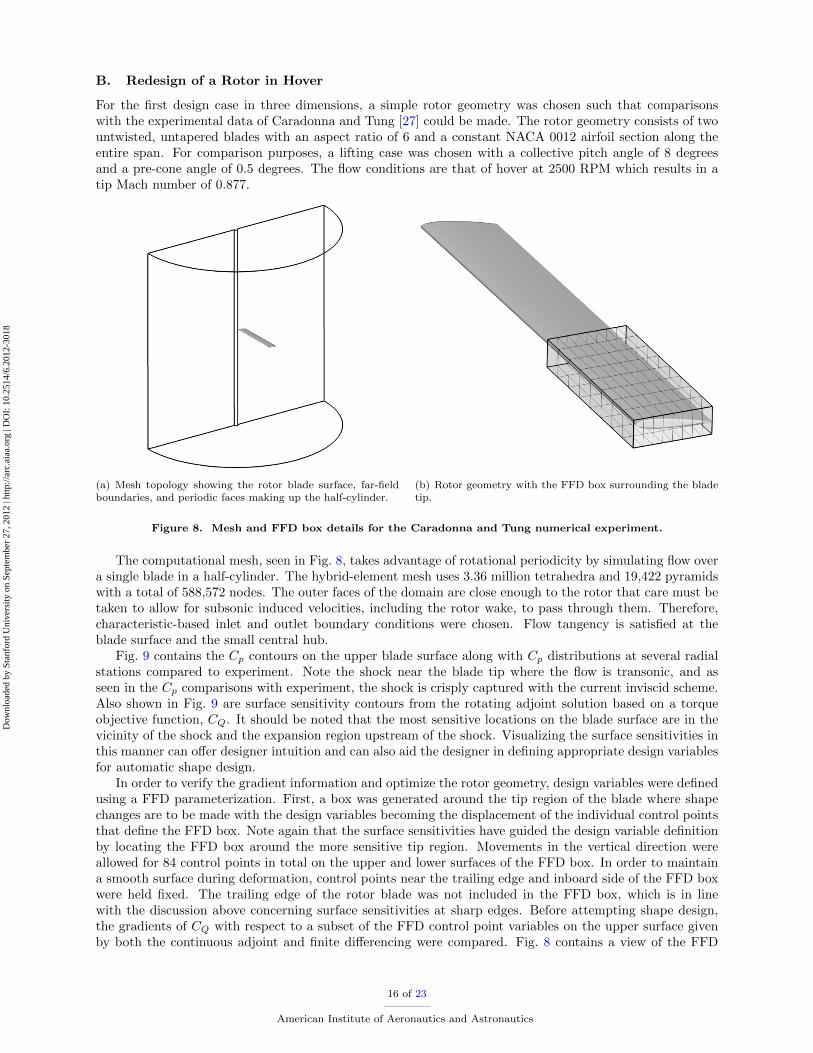
For the first design case in three dimensions, a simple rotor geometry was chosen such that comparisonswith the experimental data of Caradonna and Tung [27] could be made. The rotor geometry consists of twountwisted, untapered blades with an aspect ratio of 6 and a constant NACA 0012 airfoil section along theentire span. For comparison purposes, a lifting case was chosen with a collective pitch angle of 8 degreesand a pre-cone angle of 0.5 degrees. The flow conditions are that of hover at 2500 RPM which results in atip Mach number of 0.877.
(a) Mesh topology showing the rotor blade surface, far-fieldboundaries, and periodic faces making up the half-cylinder.
(b) Rotor geometry with the FFD box surrounding the bladetip.
Figure 8. Mesh and FFD box details for the Caradonna and Tung numerical experiment.
The computational mesh, seen in Fig. 8, takes advantage of rotational periodicity by simulating flow overa single blade in a half-cylinder. The hybrid-element mesh uses 3.36 million tetrahedra and 19,422 pyramidswith a total of 588,572 nodes. The outer faces of the domain are close enough to the rotor that care must betaken to allow for subsonic induced velocities, including the rotor wake, to pass through them. Therefore,characteristic-based inlet and outlet boundary conditions were chosen. Flow tangency is satisfied at theblade surface and the small central hub.
Fig. 9 contains the Cp
contours on the upper blade surface along with Cp
distributions at several radialstations compared to experiment. Note the shock near the blade tip where the flow is transonic, and asseen in the C
p
comparisons with experiment, the shock is crisply captured with the current inviscid scheme.Also shown in Fig. 9 are surface sensitivity contours from the rotating adjoint solution based on a torqueobjective function, C
Q
. It should be noted that the most sensitive locations on the blade surface are in thevicinity of the shock and the expansion region upstream of the shock. Visualizing the surface sensitivities inthis manner can o↵er designer intuition and can also aid the designer in defining appropriate design variablesfor automatic shape design.
In order to verify the gradient information and optimize the rotor geometry, design variables were definedusing a FFD parameterization. First, a box was generated around the tip region of the blade where shapechanges are to be made with the design variables becoming the displacement of the individual control pointsthat define the FFD box. Note again that the surface sensitivities have guided the design variable definitionby locating the FFD box around the more sensitive tip region. Movements in the vertical direction wereallowed for 84 control points in total on the upper and lower surfaces of the FFD box. In order to maintaina smooth surface during deformation, control points near the trailing edge and inboard side of the FFD boxwere held fixed. The trailing edge of the rotor blade was not included in the FFD box, which is in linewith the discussion above concerning surface sensitivities at sharp edges. Before attempting shape design,the gradients of C
Q
with respect to a subset of the FFD control point variables on the upper surface givenby both the continuous adjoint and finite di↵erencing were compared. Fig. 8 contains a view of the FFD
16 of 23
American Institute of Aeronautics and Astronautics
Dow
nloa
ded
by S
tanf
ord
Uni
vers
ity o
n Se
ptem
ber
27, 2
012
| http
://ar
c.ai
aa.o
rg |
DO
I: 1
0.25
14/6
.201
2-30
18

box around the blade tip, and the gradient comparison appears in Fig. 10. Again, while the adjoint andfinite di↵erencing gradients are not identical, they exhibit similar character and di↵erences in line withexpectations for the two approaches.
Figure 9. Cp contours on the upper surface of the initial rotor geometry and comparison to experiment atmultiple span locations. The right end is the blade tip which is rotating toward the bottom of the page. Thesurface sensitivity contours for a torque objective function are also shown. Note the high sensitivity to shapedeformations in the vicinity of the shock.
Lastly, a redesign of the rotor blade shape for minimizing torque with a minimum thrust constraint ofC
T
= 0.0055 was performed using gradient information obtained via the continuous adjoint approach. After20 design cycles, C
Q
was reduced by 26.9 % from 0.0006098 to 0.0004458 while maintaining a CT
value of0.00553 from a starting value of 0.00575. These optimization results are presented in Fig. 10. The initialand final surface shapes with C
p
contours are compared in Fig. 11. The strong shock on the upper surfacehas been removed due to a pronounced change in the shape near the tip. The optimized design features ablade tip with a sharper, downturned leading edge and a thinner, asymmetric section shape.
C. Open Rotor Blade Shape Design
Open rotor blades will operate in a transonic flow regime due to a desire for high e↵ective bypass ratios (highpropulsive e�ciency) at or slightly below current commercial aircraft cruise speeds. This has led to relativelylarge diameter rotors with swept sections to delay the development of shocks near the blade tips. As anexample for using the continuous adjoint method to design complex geometries, a generic open rotor bladeshape has been optimized for minimum inviscid torque at low-speed (take-o↵) conditions. These conditionswere chosen because the acoustic signature, another design consideration of current research interest, during
17 of 23
American Institute of Aeronautics and Astronautics
Dow
nloa
ded
by S
tanf
ord
Uni
vers
ity o
n Se
ptem
ber
27, 2
012
| http
://ar
c.ai
aa.o
rg |
DO
I: 1
0.25
14/6
.201
2-30
18

(a) Continuous adjoint and finite di↵erencing gradient com-parison for 19 FFD control point variables.
(b) Optimization results for a thrust-constrained (dotted line)inviscid torque minimization of the rotor geometry.
Figure 10. Gradient verification using the FFD control point variables and optimization results.
take-o↵ directly directly a↵ects community noise. When designing the full system, both aerodynamics andacoustics should be considered at multiple points in the flight envelope, such as during take-o↵ and cruise,and this will be addressed in future work.
A generic, 8-bladed, single rotor configuration was created, and for simplicity, the rotor is installed onan “infinite” hub. All blades are identical and were designed for a sea level thrust requirement of 10,000lbs. The thrust requirement was chosen so that if coupled with a second counter-rotating set of blades,the engine would produce approximately 20,000 lbs. of thrust and be appropriate for a typical single-aislecommercial aircraft. The blades use a NACA 65-series airfoil, and the starting rotor configuration had a4.27 m diameter with a hub-to-tip ratio of 0.36, similar to a generic configuration by Stuermer and Yin [7].The initial blade shape was designed for minimum induced losses based on blade element momentum theoryconsiderations [28] with a small modification for considering blade sweep.
The simulation again took advantage of rotational periodicity by solving for the flow about only oneof the eight blades using periodic boundary conditions. The computational mesh uses the same topologyand boundary condition specification as the Caradonna and Tung rotor case, and it consists of 387,791tetrahedra and 14,652 pyramids with a total of 79,446 nodes. The baseline geometry can be seen in Fig. 12.For performing shape design, a FFD box with the same number of control point design variables as theprevious rotor case was placed around the tip of the blade. This is also shown in Fig. 12.
A redesign of the rotor blade shape for minimizing inviscid torque with a thrust constraint was performed.Initial operating conditions were set for take-o↵ at sea level with M1 = 0.23 and an RPM of 1337, andat these conditions, a shock appears near the tip of the rotor blade. A thrust constraint of C
T
= 0.0067was imposed during the redesign in order to maintain the original design thrust of 10,000 lbs. at sea level.After 20 design cycles, C
Q
was reduced by 5.7 % from 0.002501 to 0.002357 while maintaining a CT
valueof 0.0067. These optimization results are presented in Fig. 13. The initial and final surface shapes with C
p
contours are also compared in Fig. 13. The initial shock near the trailing edge of the blade tip has beenremoved and replaced with regions of more gradual pressure variations. This example exhibits the viabilityof the method for the design of advanced geometries. Even when considering changes to only a small regionof the geometry, the designer can realize substantial performance improvements in an automatic way.
VI. Conclusions
A continuous adjoint formulation for the rotating Euler equations has been present, verified, and applied.This formulation allows for the design of rotating aerodynamic bodies in a gradient-based optimization frame-work. More specifically, the treatment given in this article is a systematic methodology for the compressibleEuler equations centered around finding surface sensitivities with the use of di↵erential geometry formulaswhich has no dependence on volume mesh sensitivities when computing the first variation of a functional
18 of 23
American Institute of Aeronautics and Astronautics
Dow
nloa
ded
by S
tanf
ord
Uni
vers
ity o
n Se
ptem
ber
27, 2
012
| http
://ar
c.ai
aa.o
rg |
DO
I: 1
0.25
14/6
.201
2-30
18

Figure 11. Comparison of the baseline and optimized rotor geometries with Cp contours. The strong shockhas been removed due to a distinct change in the tip shape.
(a) The generic open rotor geometry installed on an “infinite”hub.
(b) FFD box placement near the tip of the open rotor blade.
Figure 12. Details for the open rotor blade numerical experiment.
(only a surface integral remains). To further designer intuition, the surface sensitivities can be visualizedto clearly locate regions on the surface where shape changes will have the most e↵ect on a chosen objectivefunction. The methodology is general and could be used for the design of other rotating bodies such aspropellers, compressors, or turbines.
The continuous formulation o↵ers the advantage of physical insight into the character of the governing
19 of 23
American Institute of Aeronautics and Astronautics
Dow
nloa
ded
by S
tanf
ord
Uni
vers
ity o
n Se
ptem
ber
27, 2
012
| http
://ar
c.ai
aa.o
rg |
DO
I: 1
0.25
14/6
.201
2-30
18

(a) Cp contours on the upstream surface of the baseline andoptimized open rotor blades. The tip shock has been replacedby more gradual changes in the pressure.
(b) Optimization results for a thrust-constrained (dotted line)inviscid torque minimization.
Figure 13. Results for the open rotor blade shape design.
flow equations and their adjoint system, and in this article, the insight was used to form a modified centralscheme to alleviate convergence issues arising during the solution of the adjoint system. Along with strategiesfor defining Free-Form Deformation (FFD) variables, the new dissipation switch proposed in the modifiedcentral scheme was essential to obtaining quality solution results when performing optimal shape design.
The gradient information provided by the surface formulation has been verified for design variables intwo and three dimensions. In both situations, the gradients compared favorably with those obtained viafinite di↵erencing. In a gradient accuracy study, it was found that while the gradients obtained by finitedi↵erencing were very sensitive to design variable step sizes and solver convergence, the continuous adjointgradient information was largely insensitive to these parameters.
Optimal shape design involving the new adjoint formulation was demonstrated for three separate cases:a two-dimensional airfoil, a classic, three-dimensional rotor geometry, and open rotor blades. In each case,improvements in performance were realized, and in three dimensions, realistic thrust constraints were appliedduring optimization. Since there are few current applications of these techniques, open rotor blades representa novel application. The combination of the adjoint formulation, modified numerical solution methods onunstructured meshes, and the FFD approach o↵ers a powerful optimal shape design procedure and gives thedesigner more freedom to explore non-intuitive design spaces involving complex geometries such as highlytwisted, swept open rotor blades.
VII. Acknowledgements
T. Economon would like to acknowledge U.S. government support under and awarded by DoD, Air ForceO�ce of Scientific Research, National Defense Science and Engineering Graduate (NDSEG) Fellowship, 32CFR 168a.
References
1Reid, C., “Overview of Flight Testing of GE Aircraft Engines UDF Engine,” AIAA Paper 1988-3082, AIAA, ASME,SAE, and ASEE, Joint Propulsion Conference, 24th, Boston, Massachusetts, July 11-13, 1988.
2Sadler, J. H. R., and Hodges, G. S., “Turboprop and Open Rotor Propulsion for the Future,” AIAA Paper 1986-1472,AIAA, ASME, SAE, and ASEE, Joint Propulsion Conference, 22nd, Huntsville, Alabama, June 16-18, 1986.
20 of 23
American Institute of Aeronautics and Astronautics
Dow
nloa
ded
by S
tanf
ord
Uni
vers
ity o
n Se
ptem
ber
27, 2
012
| http
://ar
c.ai
aa.o
rg |
DO
I: 1
0.25
14/6
.201
2-30
18

3Fischer, B., and Klug, H., “Configuration Studies for a Regional Airliner Using Open-Rotor Ultra-High-Bypass-RatioEngines,” AIAA Paper 1989-2580, AIAA/ASME/SAE, and ASEE, Joint Propulsion Conference, 25th, Monterey, California,July 10-12, 1989.
4Ricouard, J., Julliard, E., Omais, M., Regnier, V., Parry, A. B., Baralon, S., “Installation e↵ects on contra-rotating openrotor noise,” AIAA 2010-3795, 16th AIAA/CEAS Aeroacoustics Conference, Stockholm, Sweden, 2010.
5Stuermer, A., “Unsteady CFD Simulations of Contra-Rotating Propeller Propulsion Systems,” AIAA 2008-5218, 44thAIAA/ASME/SAE/ASEE Joint Propulsion Conference & Exhibit, Hartford, CT, 2008.
6Deconinck, T., Ho↵er, P., Hirsch, C., De Muelenaere, A., Bonaccorsi, J., Ghorbaniasl, G., “Prediction of Near- andFar-Field Noise Generated by Contra-Rotating Open Rotors,” AIAA 2010-3794, 16th AIAA/CEAS Aeroacoustics Conference,Stockholm, Sweden, 2010.
7Stuermer, A., Yin, J., “Low-Speed Aerodynamics and Aeroacoustics of CROR Propulsion Systems,” AIAA 2009-3134,15th AIAA/CEAS Aeroacoustics Conference, Miami, FL, 2009.
8Stuermer, A., Yin, J., “Aerodynamic and Aeroacoustic Installation E↵ects for Pusher-Configuration CROR PropulsionSystems,” AIAA 2010-4235, 28th AIAA Applied Aerodynamics Conference, Chicago, IL, 2010.
9Jameson, A., “Aerodynamic Design Via Control Theory,” AIAA 81-1259, 1981.10Jameson, A., Alonso, J. J., Reuther, J., Martinelli, L., Vassberg, J. C., “Aerodynamic Shape Optimization Techniques
Based On Control Theory,” AIAA-1998-2538, 29th Fluid Dynamics Conference, Albuquerque, NM, June 15-18, 1998.11Anderson, W. K. and Venkatakrishnan, V., “Aerodynamic Design Optimization on Unstructured Grids with a Continuous
Adjoint Formulation,” Journal of Scientific Computing, Vol. 3, 1988, pp. 233-260.12Lee, S. W., Kwon, O. J., “Aerodynamic Shape Optimization of Hovering Rotor Blades in Transonic Flow Using Unstruc-
tured Meshes,” AIAA Journal, Vol. 44, No. 8, pp. 1816-1825, August, 2006.13Nielsen, E. J. Lee-Rausch, E. M. Jones, W. T., “Adjoint-Based Design of Rotors using the Navier-Stokes Equations in a
Noninertial Reference Frame,” AHS International 65th Forum and Technology Display, Grapevine, TX, May 27-29, 2009.14Dumont, A., Le Pape, A., Peter, J., Huberson, S., “Aerodynamic Shape Optimization of Hovering Rotors Using a Discrete
Adjoint of the Reynolds-Averaged Navier-Stokes Equations,” Journal of the American Helicopter Society, Vol. 56, No. 3, pp.1-11, July, 2011.
15Bueno-Orovio, A., Castro, C., Palacios, F., and Zuazua, E., “Continuous Adjoint Approach for the Spalart-AllmarasModel in Aerodynamic Optimization,” AIAA Journal , Vol. 50, No. 3, pp. 631-646, March 2012.
16Palacios, F., Alonso, J. J., Colonno, M., Hicken, J., and Lukaczyk, T., “Adjoint-Based method for supersonic aircraftdesign using equivalent area distribution,” AIAA-2012-269 , 50th AIAA Aerospace Sciences Meeting including the New HorizonsForum and Aerospace Exposition, Nashville, Tennessee, Jan. 9-12, 2012.
17Holmes, D., G., Tong, S., S., “A Three-Dimensional Euler Solver for Turbomachinery Blade Rows,” Journal of Engineeringfor Gas Turbines and Power, Vol. 107, April, 1985.
18Sokolowski, J. Zolesio, J.-P., Introduction to Shape Optimization, Springer Verlag, New York, 1991.19Baeza, A., Castro, C., Palacios, F., and Zuazua, E., “2-D Euler Shape Design on Nonregular Flows Using Adjoint
Rankine-Hugoniot Relations, AIAA Journal, Vol. 47, No. 3, pp. 552-562, 2009.20Jameson, A., Schmidt, W., and Turkel, E., “Numerical Solution of the Euler Equations by Finite Volume Methods Using
Runge-Kutta Time-Stepping Schemes,” AIAA 81-1259, 1981.21Mavriplis, D., “Accurate Multigrid Solution of the Euler Equations on Unstructured and Adaptive Meshes,” AIAA
Journal, Vol. 28, No. 2, pp. 213-221, 1990.22Venkatakrishnan, V., “Convergence to Steady State Solutions of the Euler Equations on Unstructured Grids with Lim-
iters,” Journal of Computational Physics, Vol. 118, No. 1, pp. 120-130, 1995.23Hicks, R. and Henne, P., “Wing design by numerical optimization, Journal of Aircraft, Vol. 15, pp. 407-412, 1978.24Samareh, J. A., “Aerodynamic shape optimization based on Free-Form deformation, AIAA-2004-4630, 10th
AIAA/ISSMO Multidisciplinary Analysis and Optimization Conference, Albany, New York, Aug. 2004.25Degand, C. and Farhat, C., “A three-dimensional torsional spring analogy method for unstructured dynamic meshes,
Computers & Structures, Vol. 80, pp. 305-316, 2002.26Kim, S., Alonso, J. J., Jameson, A., “A Gradient Accuracy Study for the Adjoint-Based Navier-Stokes Design Method,”
AIAA-99-0299, 37th Aerospace Sciences Meeting and Exhibit, Reno, NV, Jan. 11-14, 1999.27Caradonna, F. X., Tung, C., “Experimental and Analytical Studies of a Model Helicopter Rotor in Hover,” NASA
Technical Memorandum 81232, NASA Ames Research Center, Mo↵ett Field, CA, Sept., 1981.28Adkins, C. N., and Liebeck, R. H., “Design of Optimum Propellers,” Journal of Propulsion and Power, Vol. 10, No. 5,
pp. 676-682, 1994.
A. Transformation Matrix for Rotationally Periodic Boundary Conditions
The rotation matrix given by
T =
2
6
6
6
6
6
4
1 0 0 0 0
0 cos ✓y
cos ✓z
sin ✓x
sin ✓y
cos ✓z
� cos ✓x
sin ✓z
cos ✓x
sin ✓y
cos ✓z
+ sin ✓x
sin ✓z
0
0 cos ✓y
sin ✓z
sin ✓x
sin ✓y
sin ✓z
+ cos ✓x
cos ✓z
cos ✓x
sin ✓y
sin ✓z
� sin ✓x
cos ✓z
0
0 � sin ✓y
sin ✓x
cos ✓y
cos ✓x
cos ✓y
0
0 0 0 0 1
3
7
7
7
7
7
5
(36)
21 of 23
American Institute of Aeronautics and Astronautics
Dow
nloa
ded
by S
tanf
ord
Uni
vers
ity o
n Se
ptem
ber
27, 2
012
| http
://ar
c.ai
aa.o
rg |
DO
I: 1
0.25
14/6
.201
2-30
18

performs a periodic transformation when multiplied by the conservative variable vector, U , at one periodicface into the correct state to be applied at the matching periodic face. Note that this matrix is formed byassuming positive, right-handed rotation first about the x-axis (✓
x
), then the y-axis (✓y
), and finally thez-axis (✓
z
). It is then extended with ones in the first and last positions on the diagonal, because pointquantities such as density and energy do not require rotation in space. The same transformation matrix isused for periodic boundary conditions with the adjoint problem.
B. Linearized Solid Wall Boundary Condition
The linearized flow equations and boundary conditions are introduced during the continuous adjointderivation in order to remove any dependence on flow variations in the expression for the variation of theobjective function. The details for linearizing the solid wall boundary condition for the rotating Eulerequations are given here. We start with the flow tangency boundary condition:
(~v � ~ur
) · ~nS
= 0 on S, (37)
where ~v is the absolute flow velocity, ~ur
is the velocity due to rotation at the point on the wall, and ~nS
isthe local wall unit normal. Consider linearization with respect to small perturbations in the surface, �S, forthe both velocity and the normal terms separately,
(~v � ~ur
)0 = (~v � ~ur
) + �(~v � ~ur
) + @n
(~v � ~ur
)�S, (38)
(~nS
)0 = ~nS
+ �~nS
, (39)
where the second term on the right hand side of Eq. 38 represents the change in the flow solution causedby the deformation and the third term represents the change due solely to the geometry of the deformation.The normal of Eq. 39 does not involve the flow equations, so the only change is due to the deformation.The complete linearized boundary condition can be obtained by taking the dot product of the two linearizedcomponents,
(~v � ~ur
)0 · (~nS
)0 = {(~v � ~ur
) + �~v � �~ur
+ @n
(~v � ~ur
)�S} · (~nS
+ �~nS
)
= (~v � ~ur
) · �~nS
+ �~v · ~nS
+ @n
(~v � ~ur
)�S · ~nS
, (40)
where in order to simplify we have used the original boundary condition (Eq. 37), �~ur
= 0, and the ap-proximation that any products of variations are negligible. Keeping in mind that the linearized boundarycondition still must equal zero, Eq. 40 can be rearranged to give a useful result for the continuous adjointderivation:
�~v · ~nS
= �(~v � ~ur
) · �~nS
� @n
(~v � ~ur
) · ~nS
�S, (41)
C. Source Term Jacobian
The Jacobian of the source term appearing during the linearization of the rotating Euler equations isgiven here in both two and three dimensions. It is assumed that the reference frame is under a steadyrotation, ~! = {!
x
,!y
,!z
}T , where the three components are in the cartesian x-, y-, and z-directions. Intwo dimensions, it will be assumed that the fluid exists in the x-y plane with an angular velocity in thez-direction. The Jacobian in two dimensions is then
@Q@U
=
2
6
6
6
4
0 0 0 0
0 0 �!z
0
0 !z
0 0
0 0 0 0
3
7
7
7
5
. (42)
In three-dimensions, the steady rotation of the frame along an arbitrary axis results in the following
22 of 23
American Institute of Aeronautics and Astronautics
Dow
nloa
ded
by S
tanf
ord
Uni
vers
ity o
n Se
ptem
ber
27, 2
012
| http
://ar
c.ai
aa.o
rg |
DO
I: 1
0.25
14/6
.201
2-30
18

Jacobian:
@Q@U
=
2
6
6
6
6
6
4
0 0 0 0 0
0 0 �!z
!y
0
0 !z
0 �!x
0
0 �!y
!x
0 0
0 0 0 0 0
3
7
7
7
7
7
5
. (43)
Note that the transpose of this matrix generally appears during the solution procedure.
23 of 23
American Institute of Aeronautics and Astronautics
Dow
nloa
ded
by S
tanf
ord
Uni
vers
ity o
n Se
ptem
ber
27, 2
012
| http
://ar
c.ai
aa.o
rg |
DO
I: 1
0.25
14/6
.201
2-30
18


![InTech-Wind Turbines Theory the Betz Equation and Optimal Rotor Tip Speed Ratio[1]](https://img.pdfslide.us/doc/110x75/54300952219acdd64e8b46b0/intech-wind-turbines-theory-the-betz-equation-and-optimal-rotor-tip-speed-ratio1.jpg)