Optimal sequencing of tasks in an aluminium smelter casthouse

www.elsevier.com/locate/compind

Computers in Industry 56 (2005) 221–234

Optimal sequencing of tasks in an aluminium smelter casthouse

Pall Jensson*, Birna P. Kristinsdottir, Helgi P. Gunnarsson

Mechanical and Industrial Engineering Department, University of Iceland, Hjardarhaga 4, 107 Reykjavik, Iceland

Received 3 March 2003; received in revised form 3 November 2003; accepted 28 June 2004

Available online 16 December 2004

Abstract

This paper examines the problem of determining the sequence in which to cast aluminium ingots such that setup times are

minimized. The aluminium ingots are of different size and consist of different alloys; this poses constraints on the allowable

ordering of casting jobs. The sequencing problem can be formulated as an asymmetric traveling salesman problem with

additional constraints. Two different methods are used to formulate and solve this problem, a genetic algorithm (GA) and an

integer programming approach (IP). A new method for detecting sub-tours in the IP formulation is set forth and used. Both the

GA and IP approach are implemented in a software tool that is being used in the aluminium production industry. The results

show that even though the integer programming formulation can be used to solve the problem to optimality, the size of the

problem is a limiting factor for practical implementation. Therefore, the genetic algorithm is used in the industrial

implementation with good results.

# 2004 Elsevier B.V. All rights reserved.

Keywords: Aluminium processing; Traveling salesman problem; Genetic algorithms; Integer programming

1. Introduction

The fact that it takes a considerable amount of

energy to process aluminium makes Iceland an ideal

place for aluminium production because of the low

cost of hydropower energy. Since the first aluminium

plant was built in Iceland in 1969, production has

grown to 265.000 t per year, and further growth is

expected. The case study presented here describes a

successful use of genetic algorithms in the aluminium

* Corresponding author. Fax: +354 525 4632.

E-mail address: [email protected] (P. Jensson).

0166-3615/$ – see front matter # 2004 Elsevier B.V. All rights reserved

doi:10.1016/j.compind.2004.06.004

production industry for ISAL (the Icelandic Alumi-

nium Company owned by Alcan). We consider the

production of aluminium ingots that are produced

according to customer orders. The task of the smelter

casthouse, where the ingots are produced, is to solidify

liquid aluminium from the electrolysis, with composi-

tion, purity and form that fulfils the expectations of the

customer. The produced ingots are then loaded onto a

ship and shipped to customers. The ingots are

produced in weekly batches, as ships arrive once a

week. Each batch of orders consists of a number of

casts and the production must be scheduled in order to

minimize setup times of equipment while satisfying

some additional conditions.

.

P. Jensson et al. / Computers in Industry 56 (2005) 221–234222

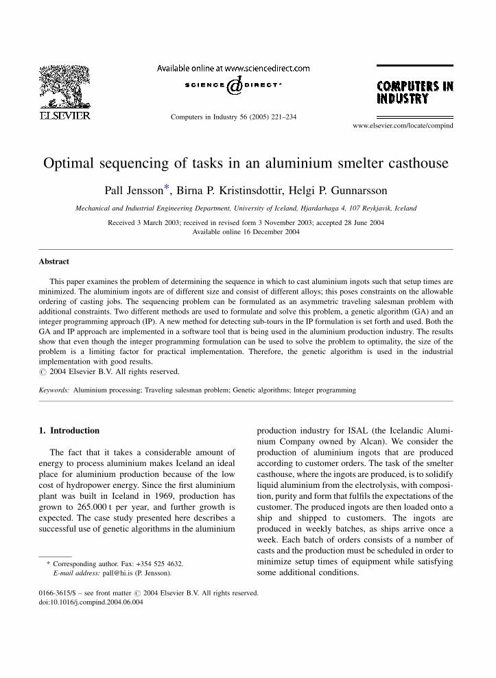
Fig. 1. The process of casting aluminium ingots.

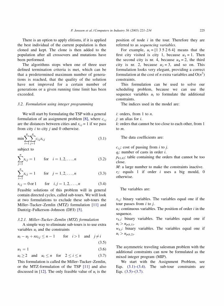
Fig. 1 illustrates the production process of

aluminium ingots. The liquid aluminium enters the

casthouse in crucibles. The liquid metal is poured into

a melting furnace; at this step scrap is added, such as

ingot ends and scrap metal from defected casts. When

the melting furnace is full the additives are added so

that the chemical composition is according to the

customer orders. Different chemical compositions are

used to obtain different properties such as strength,

viscosity and resistance to corrosion. Then the holding

time begins, when finished the furnace is ready for

casting. The aluminium is poured in launders towards

the casting machine. There are four direct casting

machines in the casthouse, and 2–7 ingots are cast at a

time on each machine. The ingots are up to 8 m long.

The casting machines are adjusted to specific

production so it is an easy job to divide the orders

between the casting machines. The sequence in which

the orders are to be cast on each casting machine is

more complex. It is important that the orders are

arranged so that the setup between casts is as small as

possible; this is done by minimizing the exchange of

moulds and launders if the orders are not identical and

casting similar alloys right after one another. In

addition to minimizing setup times, two additional

conditions must be considered:

1. F
or two of the casting machines there are not
enough mould bottoms available, so that certain

moulds have to use the same bottoms. A mechanic

is needed to exchange moulds on bottoms and this

can take considerable time. Therefore, one has to

ensure that the production planning is such that

there is enough time for this change. It is proposed

by the employees that at least 5 casts should be

between these orders. Each casting machine

produces about 5 casts a day so this should give

the mechanics enough time to change the mould

bottoms.

2. W
hen the ingots have been cast they are loaded
onto a ship. The largest ingots are put into the ship

first so that they cannot be cast after the loading has

started. Therefore, the casts that use the biggest

moulds cannot be among the last in line. A rule

used by employees is that the last 5 orders do not

use big moulds.

In the past, orders were arranged by hand. The

employee who carried out this task needed a great deal

of training and experience and the task of scheduling

casts was time-consuming. The objective of this re-

search was to develop a software tool that would

enable the employees to find a good casting schedule

quickly. We present a model implemented in a soft-

ware tool that uses genetic algorithms to create a

schedule. This allows the employee to find a good

schedule in a short time and also provides a good

schedule that utilizes the equipment at hand effec-

tively. The tool also allows for quick evaluation of

possible schedule changes when unexpected events

occur that imply a schedule change.

This paper is organized as follows. We first

describe how the problem can be formulated as an

asymmetric traveling salesman problem (ATSP) with

additional constraints. Two solution methods are used

to solve the problem, a genetic algorithm (GA) and an

integer programming (IP) approach. These two

solution procedures are compared with respect to

computation time. Finally, we describe the software

implementation.

P. Jensson et al. / Computers in Industry 56 (2005) 221–234 223

2. Formulating the problem as a traveling

salesman problem

The traveling salesman problem (TSP) is a well

known problem and widely discussed (see for instance

[4,9–13]). The TSP can be stated as follows: Given a

finite number of cities and distances between them,

find the minimum total length of a tour that visits every

city exactly once and returns to the starting city. The

TSP is symmetric if the cost cij of traveling from city i

to j is the same as from j to i. If the cost is not the same,

the problem is asymmetric (ATSP). The problem of

determining the optimal sequence of orders in our

application can be formulated as an asymmetric

traveling salesman problem (ATSP) with some

additional constraints. In the formulation, distances

in the TSP correspond to setup costs in the scheduling

problem. The problem is asymmetric because the

setup cost (distance) if an order i precedes order j is not

necessarily the same as if order j precedes i.

There are three factors that influence the setup cost

when changing from order i to j:

1. I
f orders i and j do not use the same launder.
There are two types of launders in which the

aluminium is poured from the furnace to the mould.

Some of the launders have 5 nozzles, others have 7

nozzles. Changing the launders is a relatively

simple task.

2. I
f orders i and j do not use the same mould.
The size of the ingots is determined by the

moulds. It takes more time and effort to exchange

the moulds than the launders. Each mould uses a

launder with either 5 or 7 nozzles.

3. I
f orders i and j do not consist of the same alloys
The additives in an alloy have to be within certain

limits. There are always some remains in the furnace

after each cast. Therefore, some alloys cannot be

cast right after one another without difficulty.

In addition to minimizing setup costs, two sets of

additional constraints must be considered during the

minimization. These were described in Section 1 and

are (1) orders that use big moulds cannot be among the

last 5 orders to be cast, and (2) there must be at least 5

casts between certain orders.

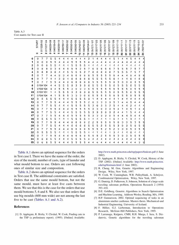
The relative setup costs have been estimated by the

employees at ISAL. An example of a cost matrix is

shown in Appendix A, see Table A.3 and [7]. The

relative cost of changing launders is 1 and the cost of

changing moulds is 3. There is also a cost when

passing from one alloy to another, these costs are

shown in [7]. This is based on the amount of each

additive in the alloys and it is also based on

experience. The cost is 0 if the composition of the

alloys is the same. In most cases the cost is between 1

and 10. Some alloys cannot be put into the furnace

right after another without emptying the furnace in

between and rinsing it. In this case the cost is

100. Here it is also evident that the problem is

asymmetric.

We have to keep in mind what moulds are in use in

the beginning and which alloys are in the furnace

when the sequence is optimized. To do that we add a

‘‘dummy’’ order to the order sequence and let it have

zero casts. This dummy order becomes the first one to

be cast. The cost of passing from the dummy is

calculated as before but the cost of passing an order to

the dummy is zero because the order before the

dummy is the last in line.

3. Solving the scheduling problem

The traveling salesman problem is difficult to solve

and several solution procedures, both exact and

heuristic, have been used to obtain a solution. In this

paper we formulate and apply two solution approaches

to our problem, a genetic algorithm which is a

heuristic method and an integer programming method

which is an exact optimization method.

3.1. Formulation using genetic algorithms

Genetic algorithms are stochastic search techni-

ques based on the mechanisms of natural selection and

natural genetics [3]. Early reports for solving TSP

using GA can be found in [6], since then genetic

algorithms have been used by many to solve traveling

salesman problems.

Genetic algorithms start with an initial set of

random solutions called population. Each individual

(solution) in the population is called a chromosome. A

chromosome is a string of symbols that represent one

point in the solution space. The chromosomes evolve

through successive iterations called generations. For


each generation, the chromosomes are evaluated,

using some measure of fitness. To create the next

generation, offspring are formed either by merging

two chromosomes from the current generation using a

crossover operator or by modifying a chromosome

using a mutation operator. A selection operator is used

to select the best individuals and reject others in order

to keep the population size constant. The general

structure of the genetic algorithms can be described as

follows:

generation = 1;initialize population;evaluate fitness;while (termination condition notsatisfied)generation = generation + 1;crossover;mutate;evaluate fitness;select;end

There are many different representations and op-

erators available. Here we will only describe the ones

we use in our implementation. In [9] several types of

operators and representations for the TSP are com-

pared. In our implementation the representation and

operators recommended and described in [9] are used.

A permutation representation is used here. The search

space for this representation is the set of permutations

of the cities. For example, a tour of an 8-city TSP 1-2-

3-4-5-6-7-8 is simply represented as follows, x = [0 1 2

3 4 5 6 7 8].

A dummy order x0 = 0 is added to account for

initial values. This value cannot be changed by

mutation or crossover. The main disadvantage with

this representation is that it makes the crossover

operator a bit complicated. Using the permutation

representation the following parameters and variables

are defined,

n: number of cities

xi: integer variables, the representation of a city i = 0,

. . ., n

cxi;xj : the cost of passing from city xi to xj

M: a large number that penalizes solutions that violate

constraints.

To evaluate the fitness of an individual in a pop-

ulation, it must be checked for feasibility. For this

purpose, two indicators g1 and g2 are defined as fol-

lows:

g1 ¼1 if orders that use the same mould

bottoms are too close

0 otherwise

8<:

1 if orders that use the big moulds are8<

g2 ¼ too late in the sequence

0 otherwise:

Assuming minimization the fitness function f(x) used

for fitness evaluation can be written as:

f ðxÞ ¼Xn

i¼1

cxi�1xiþ Mðg1 þ g2Þ

The crossover operator used is order crossover

where pc is the probability of crossover. The order

crossover works as follows. If pc is less than a random

number between 0 and 1, then the following steps are

performed.

1. S
elect a substring from one parent at random.
2. P
roduce a proto-child by copying the substring into
the corresponding positions.

3. D
elete the cities that are already in the substring
from the second parent.

4. P
lace the cities into the unfixed positions of the
proto-child from left to right according to the order

of the sequence.

To produce another offspring select a substring

from the second parent and fill in the blanks with cities

from the first one.

The mutation operator used is displacement

mutation where pm is the probability of mutation. If

pm is less than a random number between 0 and 1, then

we first select a substring at random. This substring is

removed from the tour and inserted in a random

place.

When a new generation of offspring has been

generated using the crossover and mutation operators,

tournament selection is used to select individuals that

continue on in the population. The fitness values of

two individuals selected at random are compared and

the better one is kept.


There is an option to apply elitisms, if it is applied

the best individual of the current population is then

cloned and kept. The clone is then added to the

population after all crossovers and mutations have

been performed.

The algorithms stops when one of three user

defined termination criteria is met, which can be

that a predetermined maximum number of genera-

tions is reached, that the quality of the solution

have not improved for a certain number of

generations or a given running time limit has been

exceeded.

3.2. Formulation using integer programming

We will start by formulating the TSP with a general

formulation of an assignment problem [8], where ci,j

are the distances between cities and xi,j = 1 if we pass

from city i to city j and 0 otherwise.

minXn

i¼1

Xn

j¼1

ci;jxi;j (3.1)

subject to

Xn

j¼1

xi;j ¼ 1 for i ¼ 1; 2; . . . ; n (3.2)

Xn

i¼1

xi;j ¼ 1 for j ¼ 1; 2; . . . ; n (3.3)

xi;j ¼ 0 or 1 for i; j ¼ 1; 2; . . . ; n (3.4)

Feasible solutions of this problem will in general

contain directed cycles, called sub-tours. We will look

at two formulations to exclude these sub-tours the

Miller–Tucker–Zemlin (MTZ) formulation [11] and

Dantzig–Fulkerson–Johnson (DFJ) [5].

3.2.1. Miller–Tucker–Zemlin (MTZ) formulation

A simple way to eliminate sub-tours is to use extra

variables ui and the constraints

ui � uj þ nxi;j � n � 1 for i> 1 and j 6¼ i

(3.5)

u1 ¼ 1 (3.6)

ui � 2 and ui � n for 2 � i � n (3.7)

This formulation is called the Miller–Tucker–Zemlin,

or the MTZ-formulation of the TSP [11] and also

discussed in [12]. The only feasible value of ui is the

position of node i in the tour. Therefore they are

referred to as sequencing variables.

For example, ui = [1 3 5 2 6 4] means that the

first city visited is city 1, because u1 = 1. Then

the second city is nr. 4, because u4 = 2, the third

city is nr. 2, because u2 = 3, and so on. This

formulation looks very elegant, providing a correct

formulation at the cost of n extra variables and O(n2)

constraints.

This formulation can be used to solve our

scheduling problem, because we can use the

sequence variables ui to formulate the additional

constraints.

The indices used in the model are:

i: orders, from 1 to n.

j: an alias for i.

k: orders that cannot be too close to each other, from 1

to m.

The data coefficients are:

ci,j: cost of passing from i to j.

qi: number of casts in order i.

pk1,k2: table containing the orders that cannot be too

close.

M: a large number to make the constraints inactive.

ri: equals 1 if order i uses a big mould, 0

otherwise.

The variables are:

xi,j: binary variables. The variables equal one if the

tour passes from i to j.

ui: continuous variables. The position of order i in the

sequence.

vk,i: binary variables. The variables equal one if

ui > up(k,1).

wk,i: binary variables. The variables equal one if

ui > up(k,2).

The asymmetric traveling salesman problem with the

additional constraints can now be formulated as the

mixed integer program (MIP).

We start with the Assignment Problem, see

Eqs. (3.1)–(3.4). The sub-tour constraints are

Eqs. (3.5)–(3.7).


Constraints to find the orders that are cast after pk,1

and pk,2:

Nvk;i � ui � upðk;1Þ for i ¼ 1; 2; . . . ; n

and k ¼ 1; 2; . . . ;m (3.8)

Nwk;i � ui � upðk;2Þ for i ¼ 1; 2; . . . ; n

and k ¼ 1; 2; . . . ;m (3.9)

XN

i¼1

vk;i ¼ N � upðk;1Þ for k ¼ 1; 2; . . . ;m

(3.10)

XN

i¼1

wk;i ¼ N � upðk;2Þ for k ¼ 1; 2; . . . ;m

(3.11)

vk;pðk;1Þ ¼ 0 for k ¼ 1; 2; . . . ;m (3.12)

wk;pðk;2Þ ¼ 0 for k ¼ 1; 2; . . . ;m (3.13)

We also need constraints to ensure that at least 5 casts

are between pk,1 and pk,2. Only one of these two

constraints is active depending on which order is later

in the sequence, pk,1 or pk,2:

XN

i¼1

qiðwk;i � vk;iÞ� 5 � Mvk;pðk;2Þ for

k ¼ 1; 2; . . . ;m (3.14)

XN

i¼1

qiðvk;i � wk;iÞ� 5 � Mwk;pðk;1Þ for

k ¼ 1; 2; . . . ;m (3.15)

Constraint to ensure that the last 5 orders do not use

big moulds

riui � N � 5 for i ¼ 2; 3; . . . ; n (3.16)

This formulation works well when the orders are few

but as the number of orders increases, experience

shows that the model becomes harder to solve.

Therefore we also solved the problem with the DFJ

formulation.

3.2.2. Dantzig–Fulkerson–Johnson (DFJ) branch

and cut method

Another way of eliminating sub-tours is adding the

family of sub-tour constraintsXi2 S

Xj =2 S

xi;j � 1

for all proper point subsets S; jSj � 2

(3.17)

This formulation is called the Dantzig–Fulkerson–

Johnson, or the DFJ formulation of the TSP [5] and

also discussed in [1,2]. These constraints mean that for

all possible combinations of two or more cities, S, then

at least one of the cities in S is connected to a city that

is not in S.

This is the most common formulation of the TSP

and it seems to be the only formulation that allows one

to solve large problems to optimality. The main

setback with this formulation is the vast number of

constraints. The number of constraints increases

exponentially with the problem size n, so it becomes

impossible to consider them all.

4. Sub-tour identification

The DFJ branch and cut algorithm consists of solving

a relaxed problem and then adding constraints to

eliminate solutions which are feasible to the relaxed

problem but not to the original problem. This is repeated

untilwehavea legal solution.Because thesolution to the

relaxed problem serves as a lower bound to the original

problem, we end with an optimal solution.

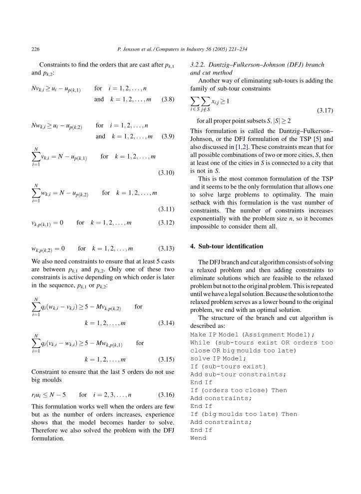
The structure of the branch and cut algorithm is

described as:

Make IP Model (Assignment Model);While (sub-tours exist OR orders tooclose OR big moulds too late)solve IP Model;If (sub-tours exist)Add sub-tour constraints;End IfIf (orders too close) ThenAdd constraints;End IfIf (big moulds too late) ThenAdd constraints;End IfWend


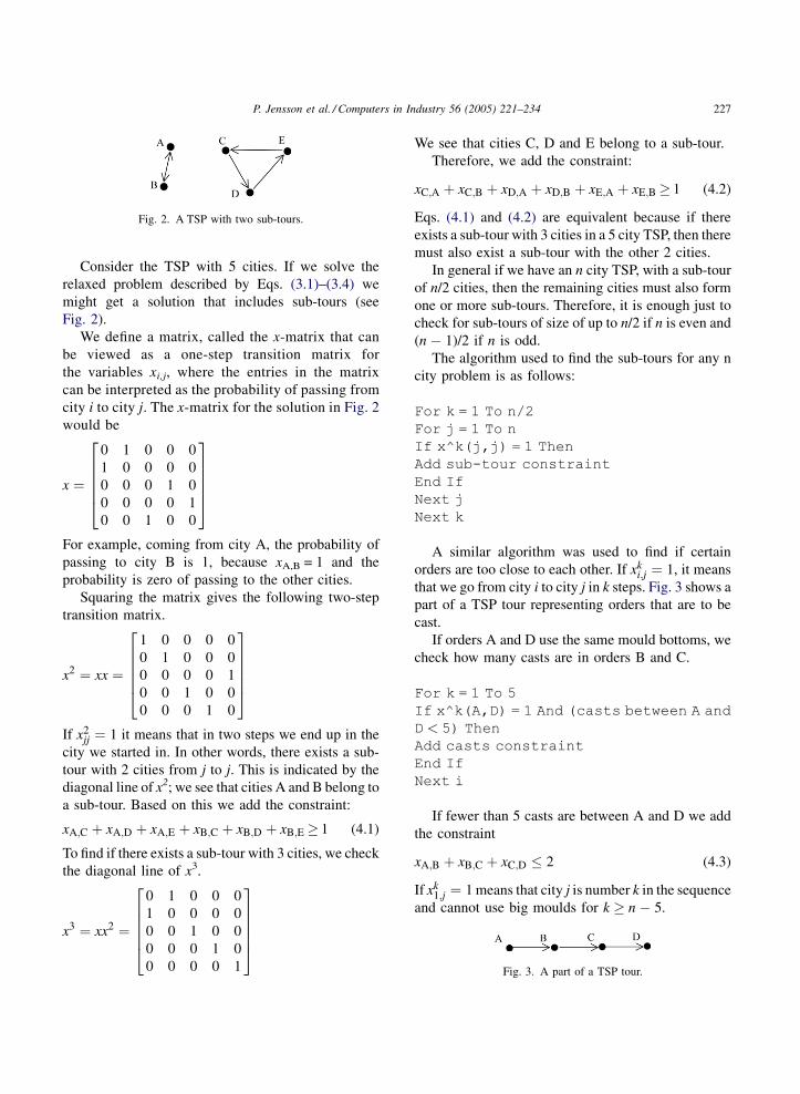
Fig. 2. A TSP with two sub-tours.

Fig. 3. A part of a TSP tour.

Consider the TSP with 5 cities. If we solve the

relaxed problem described by Eqs. (3.1)–(3.4) we

might get a solution that includes sub-tours (see

Fig. 2).

We define a matrix, called the x-matrix that can

be viewed as a one-step transition matrix for

the variables xi,j, where the entries in the matrix

can be interpreted as the probability of passing from

city i to city j. The x-matrix for the solution in Fig. 2

would be

x ¼

0 1 0 0 0

1 0 0 0 0

0 0 0 1 0

0 0 0 0 1

0 0 1 0 0

266664

377775

For example, coming from city A, the probability of

passing to city B is 1, because xA,B = 1 and the

probability is zero of passing to the other cities.

Squaring the matrix gives the following two-step

transition matrix.

x2 ¼ xx ¼

1 0 0 0 0

0 1 0 0 0

0 0 0 0 1

0 0 1 0 0

0 0 0 1 0

266664

377775

If x2jj ¼ 1 it means that in two steps we end up in the

city we started in. In other words, there exists a sub-

tour with 2 cities from j to j. This is indicated by the

diagonal line of x2; we see that cities A and B belong to

a sub-tour. Based on this we add the constraint:

xA;C þ xA;D þ xA;E þ xB;C þ xB;D þ xB;E � 1 (4.1)

To find if there exists a sub-tour with 3 cities, we check

the diagonal line of x3.

x3 ¼ xx2 ¼

0 1 0 0 0

1 0 0 0 0

0 0 1 0 0

0 0 0 1 0

0 0 0 0 1

266664

377775

We see that cities C, D and E belong to a sub-tour.

Therefore, we add the constraint:

xC;A þ xC;B þ xD;A þ xD;B þ xE;A þ xE;B � 1 (4.2)

Eqs. (4.1) and (4.2) are equivalent because if there

exists a sub-tour with 3 cities in a 5 city TSP, then there

must also exist a sub-tour with the other 2 cities.

In general if we have an n city TSP, with a sub-tour

of n/2 cities, then the remaining cities must also form

one or more sub-tours. Therefore, it is enough just to

check for sub-tours of size of up to n/2 if n is even and

(n � 1)/2 if n is odd.

The algorithm used to find the sub-tours for any n

city problem is as follows:

For k = 1 To n/2For j = 1 To nIf x^k(j,j) = 1 ThenAdd sub-tour constraintEnd IfNext jNext k

A similar algorithm was used to find if certain

orders are too close to each other. If xki;j ¼ 1, it means

that we go from city i to city j in k steps. Fig. 3 shows a

part of a TSP tour representing orders that are to be

cast.

If orders A and D use the same mould bottoms, we

check how many casts are in orders B and C.

For k = 1 To 5If x^k(A,D) = 1 And (casts between A andD < 5) ThenAdd casts constraintEnd IfNext i

If fewer than 5 casts are between A and D we add

the constraint

xA;B þ xB;C þ xC;D � 2 (4.3)

If xk1;j ¼ 1 means that city j is number k in the sequence

and cannot use big moulds for k � n � 5.


The algorithm we used to find if the big moulds are

too late in the sequence:

For i = 1 To nIf r(i) = 1 ThenFor k = n - 5 To nIf x^k(1,i) = 1 ThenAdd constraintEnd IfNext jEnd IfNext k

The constraints are of the same form as Eq. (4.3) if

we look at D as the last order and A as an order that

uses big moulds.

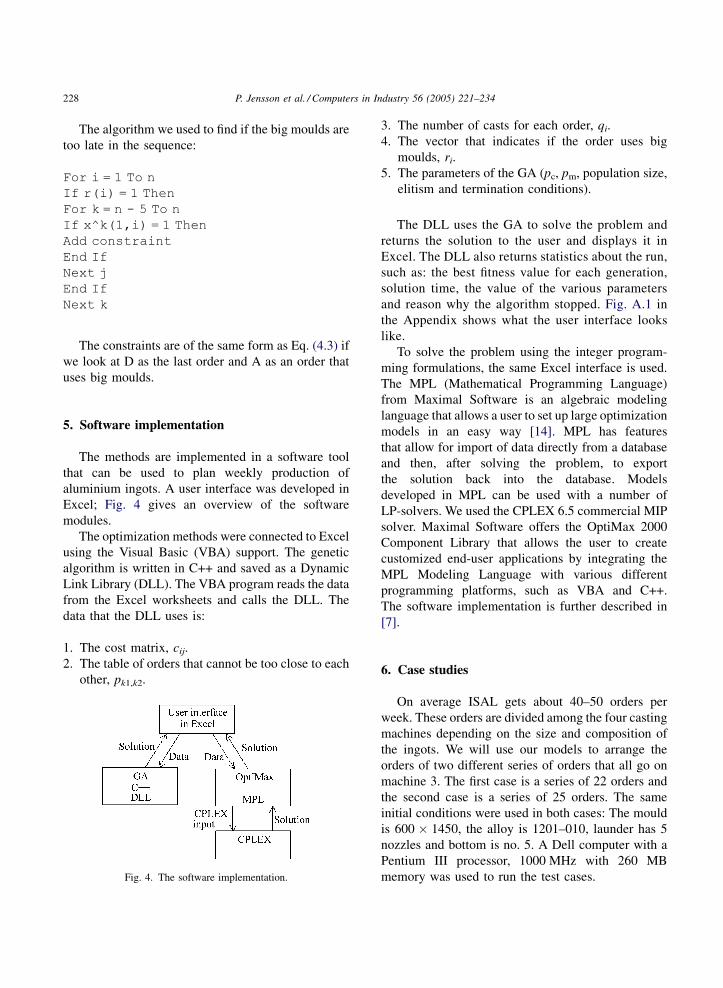
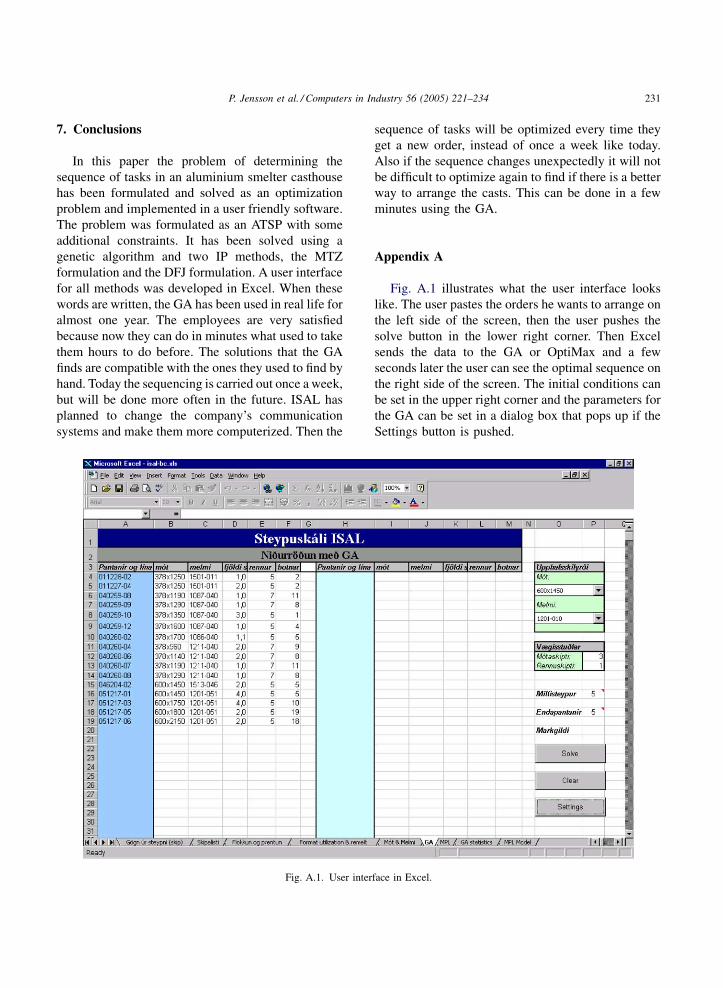
5. Software implementation

The methods are implemented in a software tool

that can be used to plan weekly production of

aluminium ingots. A user interface was developed in

Excel; Fig. 4 gives an overview of the software

modules.

The optimization methods were connected to Excel

using the Visual Basic (VBA) support. The genetic

algorithm is written in C++ and saved as a Dynamic

Link Library (DLL). The VBA program reads the data

from the Excel worksheets and calls the DLL. The

data that the DLL uses is:

1. T
he cost matrix, cij.
2. T
he table of orders that cannot be too close to each
other, pk1,k2.

Fig. 4. The software implementation.

3. T
he number of casts for each order, qi.
4. T
he vector that indicates if the order uses big
moulds, ri.

5. T
he parameters of the GA (pc, pm, population size,
elitism and termination conditions).

The DLL uses the GA to solve the problem and

returns the solution to the user and displays it in

Excel. The DLL also returns statistics about the run,

such as: the best fitness value for each generation,

solution time, the value of the various parameters

and reason why the algorithm stopped. Fig. A.1 in

the Appendix shows what the user interface looks

like.

To solve the problem using the integer program-

ming formulations, the same Excel interface is used.

The MPL (Mathematical Programming Language)

from Maximal Software is an algebraic modeling

language that allows a user to set up large optimization

models in an easy way [14]. MPL has features

that allow for import of data directly from a database

and then, after solving the problem, to export

the solution back into the database. Models

developed in MPL can be used with a number of

LP-solvers. We used the CPLEX 6.5 commercial MIP

solver. Maximal Software offers the OptiMax 2000

Component Library that allows the user to create

customized end-user applications by integrating the

MPL Modeling Language with various different

programming platforms, such as VBA and C++.

The software implementation is further described in

[7].

6. Case studies

On average ISAL gets about 40–50 orders per

week. These orders are divided among the four casting

machines depending on the size and composition of

the ingots. We will use our models to arrange the

orders of two different series of orders that all go on

machine 3. The first case is a series of 22 orders and

the second case is a series of 25 orders. The same

initial conditions were used in both cases: The mould

is 600 � 1450, the alloy is 1201–010, launder has 5

nozzles and bottom is no. 5. A Dell computer with a

Pentium III processor, 1000 MHz with 260 MB

memory was used to run the test cases.


Table 1

Reducing the number of variables

Number of variables

DFJ MTZ

22 orders 529–258 600–315

25 orders 676–463 1118–823

Table 3

Statistics for Test case II

Formulation DFJ MTZ

Continuous variables 0 24

Integer variables 463 799

Constraints 38 577

Solution time (s) 44,63 –

6.1. Solution using IP formulations

The MTZ and DFJ formulations were used to find

an optimal solution. To reduce the number of variables

in the MPL model we only declared a variable xi,j if ci,j

was reasonably low (ci,j < 6), see Table A.3 in

Appendix A. If two or more orders were identical

(use the same moulds and the same alloy) we

combined them into one order. This way we could

reduce the number of variables considerably as shown

in Table 1.

6.1.1. Test case I

In this example 22 orders are arranged. Out of these

orders, 7 orders use the same mould bottom and have

to have at least 5 casts between them. Two of the

orders use big moulds and therefore they cannot be

among the last 5 orders to be cast. Table 2 shows the

number of variables, constraints and solution times for

the DFJ and MTZ formulations, respectively. For both

formulations the same optimal sequence was obtained

with an objective function value of 48. It took

considerably longer to solve the problem using the

MTZ formulation than with the DFJ formulation. The

optimal sequence for Test case I is shown in Table A.1

in the Appendix.

6.1.2. Test case II

In the second case there are 25 orders to be

arranged. Like in test case I, 7 pairs of orders use the

same bottom and have to have at least 5 casts between

them. In this case 12 of the orders use big moulds.

Table 2

Statistics for Test case I

Formulation DFJ MTZ

Continuous variables 0 19

Integer variables 258 296

Constraints 38 405

Solution time (s) 5,45 32,92

Therefore, they cannot be among the last 5 orders to be

cast. Table 3 shows the number of variables and

constraints and solution times for both formulations.

The branch and cut method for the DFJ formulation

gave a sequence with an objective function value of

63. A solution was not obtained using the MTZ

formulation. The computer ran for a few hours, then

stopped and returned a message saying it was out of

memory. The optimal sequence found with the DFJ

formulation is shown in Table A.2 in the Appendix.

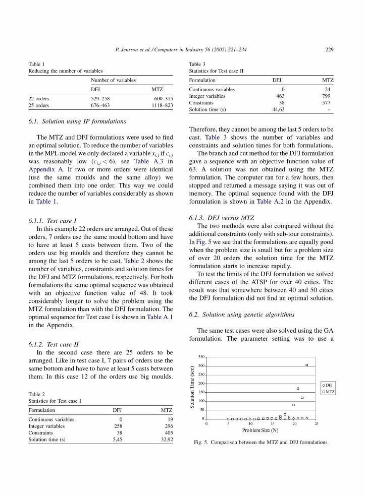
6.1.3. DFJ versus MTZ

The two methods were also compared without the

additional constraints (only with sub-tour constraints).

In Fig. 5 we see that the formulations are equally good

when the problem size is small but for a problem size

of over 20 orders the solution time for the MTZ

formulation starts to increase rapidly.

To test the limits of the DFJ formulation we solved

different cases of the ATSP for over 40 cities. The

result was that somewhere between 40 and 50 cities

the DFJ formulation did not find an optimal solution.

6.2. Solution using genetic algorithms

The same test cases were also solved using the GA

formulation. The parameter setting was to use a

Fig. 5. Comparison between the MTZ and DFJ formulations.


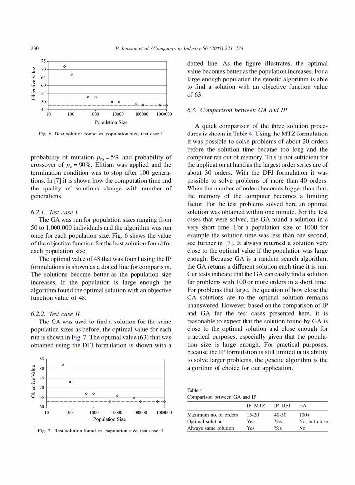
Fig. 6. Best solution found vs. population size, test case I.

probability of mutation pm = 5% and probability of

crossover of pc = 90%. Elitism was applied and the

termination condition was to stop after 100 genera-

tions. In [7] it is shown how the computation time and

the quality of solutions change with number of

generations.

6.2.1. Test case I

The GA was run for population sizes ranging from

50 to 1.000.000 individuals and the algorithm was run

once for each population size. Fig. 6 shows the value

of the objective function for the best solution found for

each population size.

The optimal value of 48 that was found using the IP

formulations is shown as a dotted line for comparison.

The solutions become better as the population size

increases. If the population is large enough the

algorithm found the optimal solution with an objective

function value of 48.

6.2.2. Test case II

The GA was used to find a solution for the same

population sizes as before, the optimal value for each

run is shown in Fig. 7. The optimal value (63) that was

obtained using the DFJ formulation is shown with a

Fig. 7. Best solution found vs. population size, test case II.

dotted line. As the figure illustrates, the optimal

value becomes better as the population increases. For a

large enough population the genetic algorithm is able

to find a solution with an objective function value

of 63.

6.3. Comparison between GA and IP

A quick comparison of the three solution proce-

dures is shown in Table 4. Using the MTZ formulation

it was possible to solve problems of about 20 orders

before the solution time became too long and the

computer ran out of memory. This is not sufficient for

the application at hand as the largest order series are of

about 30 orders. With the DFJ formulation it was

possible to solve problems of more than 40 orders.

When the number of orders becomes bigger than that,

the memory of the computer becomes a limiting

factor. For the test problems solved here an optimal

solution was obtained within one minute. For the test

cases that were solved, the GA found a solution in a

very short time. For a population size of 1000 for

example the solution time was less than one second,

see further in [7]. It always returned a solution very

close to the optimal value if the population was large

enough. Because GA is a random search algorithm,

the GA returns a different solution each time it is run.

Our tests indicate that the GA can easily find a solution

for problems with 100 or more orders in a short time.

For problems that large, the question of how close the

GA solutions are to the optimal solution remains

unanswered. However, based on the comparison of IP

and GA for the test cases presented here, it is

reasonable to expect that the solution found by GA is

close to the optimal solution and close enough for

practical purposes, especially given that the popula-

tion size is large enough. For practical purposes,

because the IP formulation is still limited in its ability

to solve larger problems, the genetic algorithm is the

algorithm of choice for our application.

Table 4

Comparison between GA and IP

IP–MTZ IP–DFJ GA

Maximum no. of orders 15-20 40-50 100+

Optimal solution Yes Yes No, but close

Always same solution Yes Yes No


7. Conclusions

In this paper the problem of determining the

sequence of tasks in an aluminium smelter casthouse

has been formulated and solved as an optimization

problem and implemented in a user friendly software.

The problem was formulated as an ATSP with some

additional constraints. It has been solved using a

genetic algorithm and two IP methods, the MTZ

formulation and the DFJ formulation. A user interface

for all methods was developed in Excel. When these

words are written, the GA has been used in real life for

almost one year. The employees are very satisfied

because now they can do in minutes what used to take

them hours to do before. The solutions that the GA

finds are compatible with the ones they used to find by

hand. Today the sequencing is carried out once a week,

but will be done more often in the future. ISAL has

planned to change the company’s communication

systems and make them more computerized. Then the

Fig. A.1. User inter

sequence of tasks will be optimized every time they

get a new order, instead of once a week like today.

Also if the sequence changes unexpectedly it will not

be difficult to optimize again to find if there is a better

way to arrange the casts. This can be done in a few

minutes using the GA.

Appendix A

Fig. A.1 illustrates what the user interface looks

like. The user pastes the orders he wants to arrange on

the left side of the screen, then the user pushes the

solve button in the lower right corner. Then Excel

sends the data to the GA or OptiMax and a few

seconds later the user can see the optimal sequence on

the right side of the screen. The initial conditions can

be set in the upper right corner and the parameters for

the GA can be set in a dialog box that pops up if the

Settings button is pushed.

face in Excel.


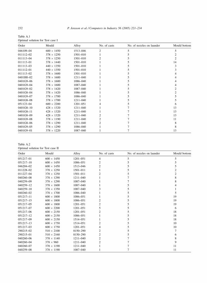
Table A.1

Optimal solution for Test case I

Order Mould Alloy No. of casts No. of nozzles on launder Mould bottom

046109–04 600 � 1450 1513–046 2 5 5

011112–02 378 � 1250 1501–010 1 5 2

011113–04 378 � 1250 1501–010 2 5 2

011113–01 378 � 1440 1501–010 1 5 14

011113–03 440 � 1350 1501–010 1 5 3

011112–01 440 � 1350 1501–010 1 5 3

011113–02 378 � 1600 1501–010 1 5 4

0401H0–02 378 � 1600 1211–040 1 5 4

0401G9–06 378 � 1600 1086–040 1 5 4

0401G9–04 378 � 1600 1087–040 1 5 4

0401G9–02 378 � 1420 1087–040 1 5 2

0401G8–04 378 � 1420 1086–040 1 5 2

0401G9–07 378 � 1700 1086–040 1 5 5

0401G8–08 378 � 1700 1211–040 1 5 5

051123–04 600 � 2200 1201–051 4 5 6

0401G8–10 428 � 1320 1211–040 1 7 13

0401G8–11 428 � 1320 1211–040 1 7 13

0401G8–09 428 � 1320 1211–040 2 7 13

0401G9–08 378 � 1190 1211–040 2 7 11

0401G8–06 378 � 1290 1211–040 2 7 8

0401G9–05 378 � 1290 1086–040 1 7 8

0401G9–01 378 � 1220 1087–040 1 7 13

Table A.2

Optimal solution for Test case II

Order Mould Alloy No. of casts No. of nozzles on launder Mould bottom

051217–01 600 � 1450 1201–051 4 5 5

051217–10 600 � 1450 1086–051 2 5 5

046204–02 600 � 1450 1513–046 2 5 5

011228–02 378 � 1250 1501–011 1 5 2

011227–04 378 � 1250 1501–011 2 5 2

040260–08 378 � 1290 1211–040 1 7 8

040259–09 378 � 1290 1087–040 1 7 8

040259–12 378 � 1600 1087–040 1 5 4

040259–10 378 � 1350 1087–040 3 5 1

040260–02 378 � 1700 1086–040 1 5 5

051217–11 600 � 1800 1086–051 1 5 19

051217–15 600 � 1800 1086–051 2 5 19

051217–05 600 � 1800 1201–051 2 5 19

051217–07 600 � 2200 1201–051 5 5 6

051217–06 600 � 2150 1201–051 2 5 18

051217–12 600 � 2150 1086–051 1 5 18

051217–09 600 � 2150 1514–051 1 5 18

051217–13 600 � 1750 1514–051 2 5 10

051217–03 600 � 1750 1201–051 4 5 10

290215–02 510 � 2100 8150–290 2 5 7

290215–01 510 � 2160 8150–290 2 5 6

040260–06 378 � 1140 1211–040 2 7 8

040260–04 378 � 960 1211–040 2 7 9

040260–07 378 � 1190 1211–040 1 7 11

040259–08 378 � 1190 1087–040 1 7 11


Table A.3

Cost matrix for Test case II

Table A.1 shows an optimal sequence for the orders

in Test case I. There we have the name of the order, the

size of the mould, number of casts, type of launder and

what mould bottom to use. Orders are cast following

ones of similar size and composition.

Table A.2 shows an optimal sequence for the orders

in Test case II. The additional constraints are satisfied.

Orders that use the same mould bottom, but not the

same mould, must have at least five casts between

them. We see that this is the case for the orders that use

mould bottoms 5, 6 and 8. We also see that orders that

use big moulds (600 mm wide) are not among the last

five to be cast (Tables A.1 and A.2).

References

[1] D. Applegate, R. Bixby, V. Chvatal, W. Cook, Finding cuts in

the TSP (a preliminary report). (1995). [Online] Available:

http://www.math.princeton.edu/tsp/papers/findcuts.pdf (1 June

2002).

[2] D. Applegate, R. Bixby, V. Chvatal, W. Cook, History of the

TSP. (2002). [Online] Available: http://www.math.princeton.

edu/tsp/histmain.html (1 June 2002).

[3] R. Cheng, M. Gen, Genetic Algorithms and Engineering

Design, Wiley, New York, 1997.

[4] W. Cook, W. Cunningham, W.R. Pulleyblank, A. Schrijver,

Combinatorial Optimization, Wiley, New York, 1997.

[5] G. Dantzig, D. Fulkerson, S. Johnson, Solution of a large scale

traveling salesman problem, Operations Research 2 (1954)

393–410.

[6] D.E. Goldberg, Genetric Algorithms in Search Optimization

and Machine Learning, Addison-Wesley, Reading, MA, 1989.

[7] H.P. Gunnarsson, 2002. Optimal sequencing of tasks in an

aluminium smelter casthouse. Masters thesis. Mechanical-and

Industrial Engineering, University of Iceland.

[8] F. Hillier, G.J. Lieberman, Introduction to Operations

Research, McGraw-Hill Publishers, New York, 1995.

[9] P. Larranaga, Kuijpers, CMH, R.H. Murga, I. Inza, S. Diz-

darevic, Genetic algorithms for the traveling salesman

http://www.math.princeton.edu/tsp/papers/findcuts.pdf

http://www.math.princeton.edu/tsp/histmain.html

http://www.math.princeton.edu/tsp/histmain.html


problem: a review of representations and operators, Artificial

Intelligence Review 13 (1999) 129–170.

[10] E.L. Lawler, J.K. Lenstra, A.H.G. Rinnoy Kan, D.B. Shmoys,

The Traveling Salesman Problem. A guided Tour of Combi-

natorial Optimization, Wiley, 1985.

[11] C.E. Miller, A.W. Tucker, R.A. Zemlin, Integer Programming

Formulations of the Traveling Salesman Problem, Journal of

the Association for Computing Machinery 7 (1960) 326–329.

[12] G. Pataki, The bad and the good-and-ugly: formulations for the

traveling salesman problem. Technical Report CORC 2000-1,

2000.

[13] R.L. Rardin, Optimization in Operations Research, Prentice

Hall, New York, 1997.

[14] MPL Modeling System. (2002). [Online]. Available: http://

www.maximalsoftware.com/mpl [2002, June 1].

Dr. Pall Jensson received his B.Sc. in

Mechanical Engineering from the Uni-

versity of Iceland in 1969 and M.Sc.

and Ph.D. in Industrial Engineering with

focus on Operations Research from the

Technical University of Denmark in 1972

and 1975. From 1975 he worked with

IBM in Iceland for 2 years and between

1997 and 1986 he was the Director of

Computing Services at the University of

Iceland. Since, 1987 he has been a professor of Industrial Engineer-

ing at the same University.

Dr. Birna P. Kristinsdottir received her

B.Sc. in Mechanical Engineering from

the University of Iceland in 1991. She

received her M.Sc. and Ph.D. in Industrial

Engineering with focus on Operations

Research and Global Optimization

from the University of Washington in

1993 and 1997, respectively. From

1997 to 1998 she worked as a mathe-

matics and simulation expert at

Boeing and worked in consulting for Microsoft customer support

centers in 1999. From 1998 to 2000 she also worked as a part time

lecturer and research associate at the Department of Industrial

Engineering at the University of Washington in Seattle. She

was an Associate Professor in Industrial Engineering at the Uni-

versity of Iceland 2000–2003. She currently works at Alcan Iceland

Ltd.

Helgi Petur Gunnarsson received the

M.Sc. degree in Industrial Engineering

from The University of Iceland in 2002.

Since graduation he has worked with

logistics and modeling for various com-

panies in Iceland.

http://www.maximalsoftware.com/mpl

http://www.maximalsoftware.com/mpl

Documents

Optimal sequencing of tasks in an aluminium smelter casthouse