Optimal Monetary and Fiscal Policy at the Zero Lower Bound in a

Small Open Economy∗

Saroj Bhattarai

Penn State

Konstantin Egorov†

Penn State

Abstract

We study optimal monetary and fiscal policy at the zero lower bound in a small open econ-

omy model with sticky prices and a flexible exchange rate. In such a liquidity trap situation,

the economy suffers from a negative output gap, producer price deflation, and an appreciated

real exchange rate (compared to its efficient level). The extent of these adverse effects and the

duration of the liquidity trap is higher, lower is the elasticity of substitution between domestic

and foreign goods. Under discretion, compared to commitment, in addition to the usual “defla-

tion bias” present in a closed economy, the equilibrium in a small open economy also features

an “overvaluation bias”: the real exchange rate is excessively appreciated compared to its ef-

ficient level. Countercyclical fiscal policy, that is, increasing government spending above the

efficient level during the liquidity trap, constitutes optimal policy and helps decrease the extent

of negative output gap and deflation, especially under discretion, but the extent of the increase

in government spending is lower when the elasticity of substitution of between domestic and

foreign goods is higher.

JEL Classification: E31, E52, E58; E61; E62; E63; F41

Keywords: Optimal monetary policy; Optimal fiscal policy; Zero lower bound; Liquidity

trap; Small open economy; Commitment; Discretion

∗Preliminary. We thank Penn State brown bag seminar participants and CESifo Global Economy Area conferenceparticipants for helpful comments and sugestions. This version: May 2014.†Bhattarai: 615 Kern Building, Pennsylvania State University, University Park, PA 16802; sub31@psu.edu.

Egorov: 303 Kern Building, Pennsylvania State University, University Park, PA 16802; kze112@psu.edu.

1

1 Introduction

As a response to the recent global financial crisis and its adverse consequences on output and em-

ployment, several central banks of small open economies engaged in countercyclical policy response

and lowered their conventional policy instrument, the short-term nominal interest rate. Many of

these central banks, such as the Bank of England, the Bank of Canada, and the Bank of Japan, in

fact, found themselves frustrated by the zero lower bound (ZLB) on the short-term nominal interest

rate and thereby, unable to provide further conventional policy accommodation.

Such a development has raised several questions such as: what constitutes optimal monetary

policy when a small open economy finds itself in a liquidity trap situation, where the short-term

nominal interest rate has been lowered all the way to zero and cannot be lowered further; is there a

significant difference in equilibrium outcomes when the central bank can commit to future actions

compared to when it cannot; and, what is the role of the elasticity of substitution between domestic

and foreign goods and real exchange rate dynamics in driving equilibrium outcomes? Moreover,

given the constraints imposed by the zero lower bound on conventional monetary policy, another

natural question that arises is whether fiscal policy, in particular, countercyclical government spend-

ing, can be optimal and welfare-improving.

Motivated by these considerations, we study optimal monetary and fiscal policy at zero nom-

inal interest rates, both with and without commitment on the part of the government, in a small

open economy with sticky prices and a flexible exchange rate. In particular, we consider a general

environment without restrictions on some key model parameters which ensures that the optimal

policy problem in an open economy is no longer isomorphic to the closed economy.1 This implies for

example, that the government’s objective, which is to maximize the representative household’s util-

ity, cannot be summarized purely by home inflation and output gap stabilization.2 This difference

from the closed economy arises because there exists a standard motive related to optimal terms of

trade manipulation as the small open economy produces a good that is an imperfect substitute of

the foreign good. Overall, in this general environment, monetary policy cannot achieve the efficient

outcome, even at positive interest rates, in the presence of standard technology or preference shocks

and there is a role for fiscal policy, even at positive interest rates, as government spending optimally

deviates from its efficient level.

We show that when the small open economy is in a liquidity trap, it experiences a negative

output gap, producer price deflation, and a negative real exchange rate gap (that is, a real exchange

rate that is appreciated compared to its efficient level).3 The extent of these adverse effects and

the duration of the liquidity trap is higher, lower is the elasticity of substitution between domestic

and foreign goods. This is so because when the elasticity of substitution between domestic and

1As we discuss later, the key model parameters are the intertemporal elasticity of substitution and the elasticityof substitution between home and foreign goods.

2Moreover, the equilibrium does not necessarily feature balanced trade.3As is standard in open economy models, an increase of the exchange rate implies a depreciation in our model

and by home or producer inflation, we refer to inflation of home produced goods. Moreover, throughout the paper,we refer to a “gap”as the difference between a variable and its efficient counterpart.

2

foreign goods is lower, equilibrium requires a higher response of relative prices to clear the goods

market. In a liquidity trap situation, since the price adjustment channel gets severely impaired,

this implies that the economy suffers from a bigger output gap, producer price deflation, and a

real exchange rate gap. As a result of these adverse effects, optimal monetary policy, both with

and without commitment, keeps nominal interest rates at zero for longer when the elasticity of

substitution between domestic and foreign goods is lower. Thus, the duration of liquidity trap

depends importantly on trade elasticity in a small open economy.

We find that optimal policy under commitment, like in a closed economy, can be expressed in

terms of a suitably defined time-varying price-level target that features history dependence, while

optimal policy under discretion is purely forward looking. The equilibrium under commitment,

compared to discretion, then features a less severe negative output gap and producer price deflation.

Thus, the usual “deflation bias” of discretionary policy at the ZLB that is present in a closed

economy is also a feature of the small open economy. In particular, under commitment, the central

bank is able to promise low real interest rates and a higher output gap in future, which helps

mitigate the extent of the negative output gap during the liquidity trap. In a small open economy

environment, there is in addition, also a “overvaluation bias” associated with discretionary policy:

the real exchange rate is relatively more appreciated. Thus, under optimal policy with commitment,

the central bank also promises a more depreciated real exchange rate.4

While the commitment outcome is superior to discretion, it is well-known that it suffers from

dynamic time inconsistency: the central bank has incentives to renege on its promises in future.

We therefore, next analyze joint conduct of optimal monetary and fiscal policy, where the gov-

ernment also chooses optimally the level of (utility-yielding) government spending, an action that

involves current actions. Intuitively, increasing government spending during the liquidity trap

and/or promising to decrease it in future can be beneficial as it reduces the real interest rate gap,

that is one of the main reasons behind adverse outcomes at the ZLB. The reason is that such a

path of government spending increases the efficient real interest rate, thereby decreasing the real

interest rate gap.

We indeed show that increasing government spending above the efficient level helps decrease

adverse outcomes during the liquidity trap, especially under discretion. Optimal fiscal policy thus

entails countercyclical government spending, as in a closed economy. In particular, the extent of

negative output gap, producer price deflation, and negative real exchange rate gap gets mitigated

with higher government spending. Under discretion, government spending increases during the

liquidity trap by more compared to commitment while at the same time, unlike commitment,

the government spending gap does not go negative in later periods. The reason is that once the

government cannot commit, to achieve its goal of decreasing the real interest rate gap, it cannot

promise to a negative government spending gap in future. Thus, it solely has to rely on a higher

level of government spending today.

4Note that this does not necessarily imply that net exports is higher under commitment. This depends on thetrade elasticity.

3

Finally, under both commitment and discretion, the extent of the optimal increase in government

spending beyond the efficient level decreases when the elasticity of substitution between domestic

and foreign goods is higher. This is because the increase in government spending generates real

exchange rate appreciation pressures (and thus increases the government spending gap), which

reduces welfare more when the trade elasticity is higher.

Our contribution is to study optimal monetary and fiscal policy, both with and without com-

mitment, in a general small open economy environment, with the main focus on a situation where

the ZLB on the short-term nominal interest rate binds. Thus, we are clearly building on a recently

burgeoning literature on optimal policy at the ZLB, which is mostly based on closed economy mod-

els. In particular, our work is closely related to the set of papers that study optimal monetary and

government spending policy in a liquidity trap. Important contributions on optimal monetary pol-

icy in a liquidity trap situation in a closed economy context, either under commitment or discretion

or both, include Eggertsson and Woodford (2003), Jung, Teranishi, Watanabe (2005), Adam and

Billi (2006 and 2007), and Werning (2013). Relatedly, Eggertsson (2006) highlights the “deflation

bias” of discretionary policy at zero interest rates and suggests issuing nominal debt as a way to

improve on outcomes. In studying the role for government spending in a liquidity trap situation,

our work is related to that of Eggertsson (2001) and Werning (2013), who point out the efficacy of

countercyclical government spending policy in closed economy models.

In the open economy literature, using two-country models, Jeanne (2009) and Cook and Dev-

ereux (2013) study optimal policy, where countries coordinate on their actions, in a global liquidity

trap scenario. Our environment of a small open economy provides a different focus, as only the

home country is in a liquidity trap situation and it decides on optimal policy taking the rest of

the world as given (on which, it exerts a negligible effect). A separate policy relevant role for the

terms of trade (or the real exchange rate) in this environment is also a new feature. Our work is

closely related to that of Svensson (2003 and 2004) and Jeanne and Svensson (2007), who also use

a small open economy model and provide insights related to exchange rate dynamics and how to

mitigate adverse outcomes under discretion. The main difference is that we consider an explicitly

welfare maximizing government in characterizing optimal monetary and fiscal policy.5 In terms of

methodology, our small open economy set-up is very similar to that of Gali and Monacelli (2005),

Faia and Monacelli (2008), and De Paoli (2009), which we augment with a role for government

spending when we consider optimal fiscal policy

5In the interest of space, we only discuss the literature that focusses on optimal policy in a liquidity trap, butthere is by now also a large literature that analyzes various policy relevant issues, such as the effects of governmentspending, while modelling monetary policy as being governed by a Taylor type rule. Important contributions include,among others, closed economy studies by Wolman (2005), Eggertsson (2011), Christiano, Eichenbaum, and Rebelo(2011), Woodford (2011), and Ercez and Linde (2014), a two-country study by Bodenstein, Erceg, and Guerrieri(2009), and a current union model by Eggertsson, Ferrero, and Raffo (2013).

4

2 Model

There are two countries, home (H) and foreign (F ). The home country is a small open economy.

The foreign country is effectively a closed economy as the home country variables have negligible

effects on foreign variables.

2.1 Private sector

We first describe the environment faced by households and firms, their optimization problem, and

the associated equilibrium conditions. Our model is a standard sticky price set-up along the lines

of Woodford (2003). Moreover, it is similar to the small open economy set-up in Faia and Monacelli

(2008), augmented with a role for government spending as in Woodford (2003).

2.1.1 Households

A household at home maximizes expected discounted utility over the infinite horizon

Et

∞∑s=0

βsUt+s = Et

∞∑s=0

βs[u (Ct+s, ξt+s)−

ˆ 1

0v (ht+s(i), ξt+s) di+ g (Gt+s, ξt+s)

](1)

where β is the discount factor, Ct is household consumption of the composite final good, ht(i) is

quantity suppled of labor of type i, Gt is government consumption of the composite final good,

and ξt is a vector of aggregate exogenous (domestic) shocks. Et is the mathematical expectation

operator conditional on period-t information, u (.) is concave and strictly increasing in Ct for any

possible value of ξt, g (.) is concave and strictly increasing in Gt for any possible value of ξt,

and v (.) is increasing and convex in ht(i) for any possible value of ξt.

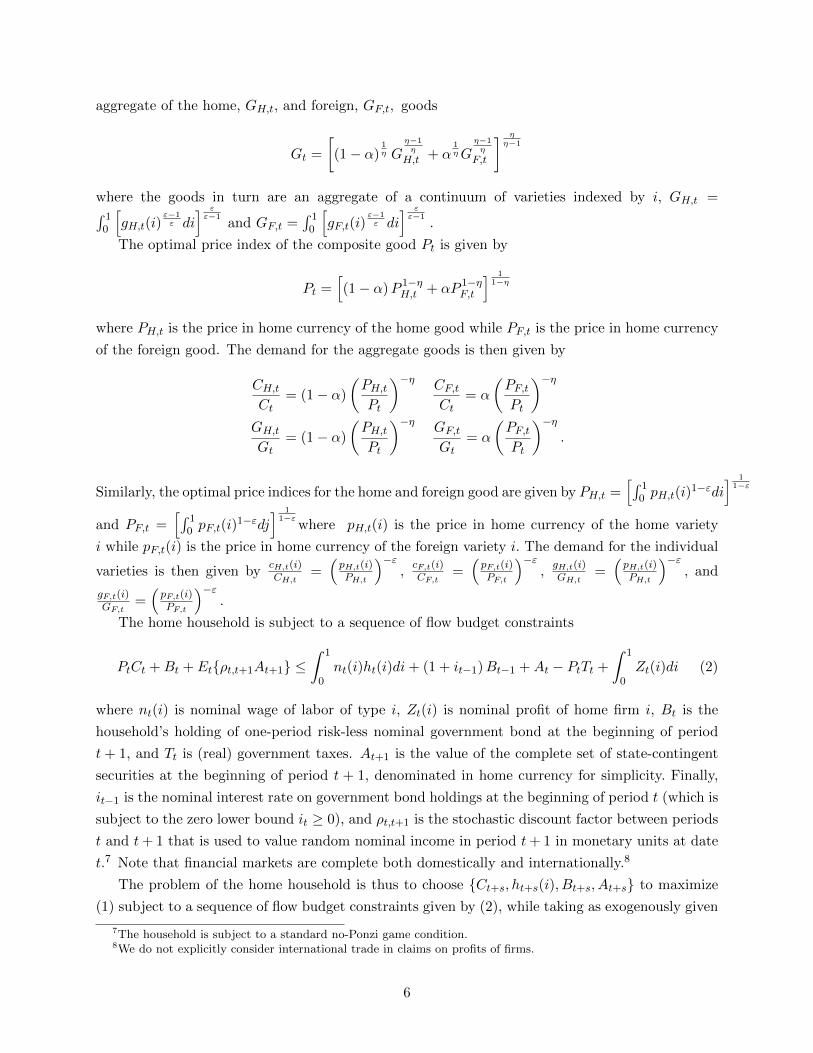
The composite household final good is an aggregate of the home, CH,t, and foreign, CF,t, goods

Ct =

[(1− α)

1η C

η−1η

H,t + α1ηC

η−1η

F,t

] ηη−1

where the goods in turn are a standard aggregate of a continuum of varieties indexed by i, CH,t =´ 10

[cH,t(i)

ε−1ε di

] εε−1

and CF,t =´ 1

0

[cF,t(i)

ε−1ε di

] εε−1

. Here, η > 0 is the elasticity of substitution

between the goods, ε > 1 is the elasticity of substitution among the varieties, and α < 1 denotes the

weight of the foreign, imported good in the home basket and therefore, is the degree of openness.6

For simplicity, we assume that the composite government final good is defined similarly as an

6Note here that for simplicity, we impose the “small open economy limit” already in defining the con-sumption bundles. A more general notation, following Faia and Monacelli (2008) would be to write Ct =[(

1− α′) 1ηCη−1η

H,t + α′ 1ηC

η−1η

F,t

] ηη−1

with α′

= (1 − n)α, where n is the size and α the trade openness of the home

country. Then, n→ 0 would constitue the “small open economy limit.”

5

aggregate of the home, GH,t, and foreign, GF,t, goods

Gt =

[(1− α)

1η G

η−1η

H,t + α1ηG

η−1η

F,t

] ηη−1

where the goods in turn are an aggregate of a continuum of varieties indexed by i, GH,t =´ 10

[gH,t(i)

ε−1ε di

] εε−1

and GF,t =´ 1

0

[gF,t(i)

ε−1ε di

] εε−1

.

The optimal price index of the composite good Pt is given by

Pt =[(1− α)P 1−η

H,t + αP 1−ηF,t

] 11−η

where PH,t is the price in home currency of the home good while PF,t is the price in home currency

of the foreign good. The demand for the aggregate goods is then given by

CH,tCt

= (1− α)

(PH,tPt

)−η CF,tCt

= α

(PF,tPt

)−ηGH,tGt

= (1− α)

(PH,tPt

)−η GF,tGt

= α

(PF,tPt

)−η.

Similarly, the optimal price indices for the home and foreign good are given by PH,t =[´ 1

0 pH,t(i)1−εdi

] 11−ε

and PF,t =[´ 1

0 pF,t(i)1−εdj

] 11−ε

where pH,t(i) is the price in home currency of the home variety

i while pF,t(i) is the price in home currency of the foreign variety i. The demand for the individual

varieties is then given bycH,t(i)CH,t

=(pH,t(i)PH,t

)−ε,cF,t(i)CF,t

=(pF,t(i)PF,t

)−ε,gH,t(i)GH,t

=(pH,t(i)PH,t

)−ε, and

gF,t(i)GF,t

=(pF,t(i)PF,t

)−ε.

The home household is subject to a sequence of flow budget constraints

PtCt +Bt + Et{ρt,t+1At+1} ≤ˆ 1

0nt(i)ht(i)di+ (1 + it−1)Bt−1 +At − PtTt +

ˆ 1

0Zt(i)di (2)

where nt(i) is nominal wage of labor of type i, Zt(i) is nominal profit of home firm i, Bt is the

household’s holding of one-period risk-less nominal government bond at the beginning of period

t + 1, and Tt is (real) government taxes. At+1 is the value of the complete set of state-contingent

securities at the beginning of period t + 1, denominated in home currency for simplicity. Finally,

it−1 is the nominal interest rate on government bond holdings at the beginning of period t (which is

subject to the zero lower bound it ≥ 0), and ρt,t+1 is the stochastic discount factor between periods

t and t+ 1 that is used to value random nominal income in period t+ 1 in monetary units at date

t.7 Note that financial markets are complete both domestically and internationally.8

The problem of the home household is thus to choose {Ct+s, ht+s(i), Bt+s, At+s} to maximize

(1) subject to a sequence of flow budget constraints given by (2), while taking as exogenously given

7The household is subject to a standard no-Ponzi game condition.8We do not explicitly consider international trade in claims on profits of firms.

6

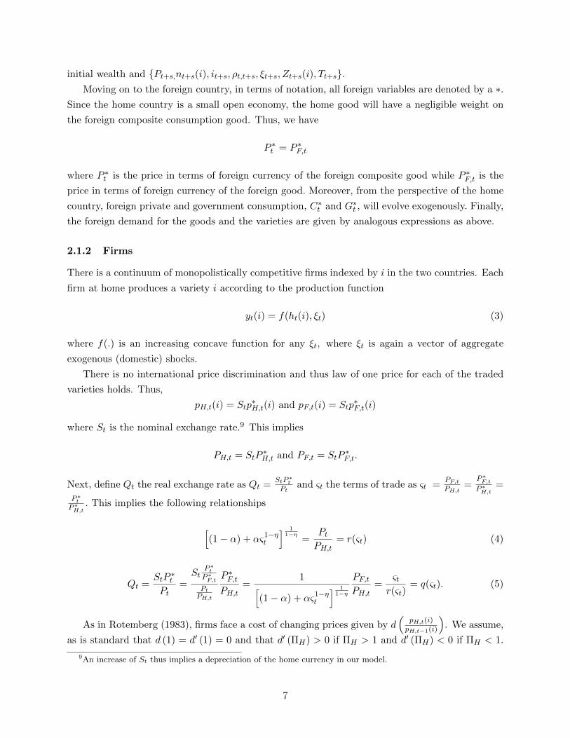
initial wealth and {Pt+s,nt+s(i), it+s, ρt,t+s, ξt+s, Zt+s(i), Tt+s}.Moving on to the foreign country, in terms of notation, all foreign variables are denoted by a ∗.

Since the home country is a small open economy, the home good will have a negligible weight on

the foreign composite consumption good. Thus, we have

P ∗t = P ∗F,t

where P ∗t is the price in terms of foreign currency of the foreign composite good while P ∗F,t is the

price in terms of foreign currency of the foreign good. Moreover, from the perspective of the home

country, foreign private and government consumption, C∗t and G∗t , will evolve exogenously. Finally,

the foreign demand for the goods and the varieties are given by analogous expressions as above.

2.1.2 Firms

There is a continuum of monopolistically competitive firms indexed by i in the two countries. Each

firm at home produces a variety i according to the production function

yt(i) = f(ht(i), ξt) (3)

where f(.) is an increasing concave function for any ξt, where ξt is again a vector of aggregate

exogenous (domestic) shocks.

There is no international price discrimination and thus law of one price for each of the traded

varieties holds. Thus,

pH,t(i) = Stp∗H,t(i) and pF,t(i) = Stp

∗F,t(i)

where St is the nominal exchange rate.9 This implies

PH,t = StP∗H,t and PF,t = StP

∗F,t.

Next, define Qt the real exchange rate as Qt =StP ∗tPt

and ςt the terms of trade as ςt =PF,tPH,t

=P ∗F,tP ∗H,t

=

P ∗tP ∗H,t

. This implies the following relationships

[(1− α) + ας1−η

t

] 11−η

=PtPH,t

= r(ςt) (4)

Qt =StP

∗t

Pt=St

P ∗tP ∗F,tPtPH,t

P ∗F,tPH,t

=1[

(1− α) + ας1−ηt

] 11−η

PF,tPH,t

=ςtr(ςt)

= q(ςt). (5)

As in Rotemberg (1983), firms face a cost of changing prices given by d(

pH,t(i)pH,t−1(i)

). We assume,

as is standard that d (1) = d′ (1) = 0 and that d′ (ΠH) > 0 if ΠH > 1 and d′ (ΠH) < 0 if ΠH < 1.

9An increase of St thus implies a depreciation of the home currency in our model.

7

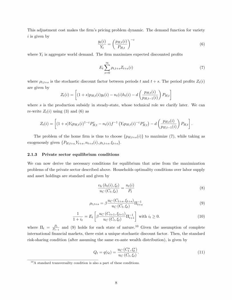
This adjustment cost makes the firm’s pricing problem dynamic. The demand function for variety

i is given byyt(i)

Yt=

(pH,t(i)

PH,t

)−ε(6)

where Yt is aggregate world demand. The firm maximizes expected discounted profits

Et

∞∑s=0

ρt,t+sZt+s(i) (7)

where ρt,t+s is the stochastic discount factor between periods t and t+ s. The period profits Zt(i)

are given by

Zt(i) =

[(1 + s)pH,t(i)yt(i)− nt(i)ht(i)− d

(pH,t(i)

pH,t−1(i)

)PH,t

]where s is the production subsidy in steady-state, whose technical role we clarify later. We can

re-write Zt(i) using (3) and (6) as

Zt(i) =

[(1 + s)YtpH,t(i)

1−εP εH,t − nt(i)f−1(YtpH,t(i)

−εP εH,t)− d

(pH,t(i)

pH,t−1(i)

)PH,t

].

The problem of the home firm is thus to choose {pH,t+s(i)} to maximize (7), while taking as

exogenously given {PH,t+s,Yt+s, nt+s(i), ρt,t+s, ξt+s}.

2.1.3 Private sector equilibrium conditions

We can now derive the necessary conditions for equilibrium that arise from the maximization

problems of the private sector described above. Households optimality conditions over labor supply

and asset holdings are standard and given by

vh (ht(i), ξt)

uC (Ct, ξt)=nt(i)

Pt(8)

ρt,t+s = βuC (Ct+s, ξt+s)

uC (Ct, ξt)Π−1t+s (9)

1

1 + it= Et

[βuC (Ct+1, ξt+1)

uC (Ct, ξt)Π−1t+1

]with it ≥ 0. (10)

where Πt = PtPt−1

and (9) holds for each state of nature.10 Given the assumption of complete

international financial markets, there exist a unique stochastic discount factor. Then, the standard

risk-sharing condition (after assuming the same ex-ante wealth distribution), is given by

Qt = q(ςt) =uC (C∗t , ξ

∗t )

uC (Ct, ξt). (11)

10A standard transversality condition is also a part of these conditions.

8

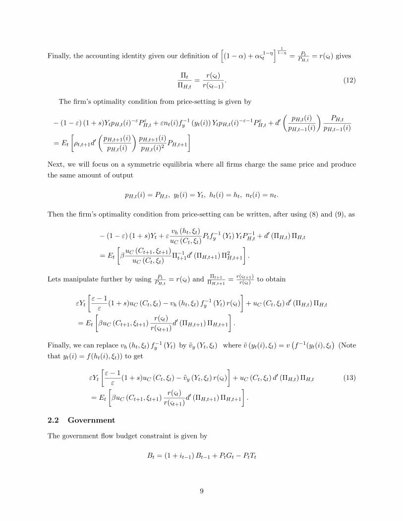
Finally, the accounting identity given our definition of[(1− α) + ας1−η

t

] 11−η

= PtPH,t

= r(ςt) gives

Πt

ΠH,t=

r(ςt)

r(ςt−1). (12)

The firm’s optimality condition from price-setting is given by

− (1− ε) (1 + s)YtpH,t(i)−εP εH,t + εnt(i)f

−1y (yt(i))YtpH,t(i)

−ε−1P εH,t + d′(

pH,t(i)

pH,t−1(i)

)PH,t

pH,t−1(i)

= Et

[ρt,t+1d

′(pH,t+1(i)

pH,t(i)

)pH,t+1(i)

pH,t(i)2PH,t+1

]Next, we will focus on a symmetric equilibria where all firms charge the same price and produce

the same amount of output

pH,t(i) = PH,t, yt(i) = Yt, ht(i) = ht, nt(i) = nt.

Then the firm’s optimality condition from price-setting can be written, after using (8) and (9), as

− (1− ε) (1 + s)Yt + εvh (ht, ξt)

uC (Ct, ξt)Ptf

−1y (Yt)YtP

−1H,t + d′ (ΠH,t) ΠH,t

= Et

[βuC (Ct+1, ξt+1)

uC (Ct, ξt)Π−1t+1d

′ (ΠH,t+1) Π2H,t+1

].

Lets manipulate further by using PtPH,t

= r(ςt) and Πt+1

ΠH,t+1= r(ςt+1)

r(ςt)to obtain

εYt

[ε− 1

ε(1 + s)uC (Ct, ξt)− vh (ht, ξt) f

−1y (Yt) r(ςt)

]+ uC (Ct, ξt) d

′ (ΠH,t) ΠH,t

= Et

[βuC (Ct+1, ξt+1)

r(ςt)

r(ςt+1)d′ (ΠH,t+1) ΠH,t+1

].

Finally, we can replace vh (ht, ξt) f−1y (Yt) by vy (Yt, ξt) where v (yt(i), ξt) = v

(f−1(yt(i), ξt

)(Note

that yt(i) = f(ht(i), ξt)) to get

εYt

[ε− 1

ε(1 + s)uC (Ct, ξt)− vy (Yt, ξt) r(ςt)

]+ uC (Ct, ξt) d

′ (ΠH,t) ΠH,t (13)

= Et

[βuC (Ct+1, ξt+1)

r(ςt)

r(ςt+1)d′ (ΠH,t+1) ΠH,t+1

].

2.2 Government

The government flow budget constraint is given by

Bt = (1 + it−1)Bt−1 + PtGt − PtTt

9

where in terms of notation, for simplicity, we are assuming that all government debt is held do-

mestically. We assume that lump-sum taxes are available and so government debt dynamics is

irrelevant for the non-fiscal variables. We thus abstract from it later in the paper. We describe the

objectives and the problem faced by the government in the next section.

2.3 Market clearing and net exports

Given that the law of one price holds, it is straightforward to derive an exact non-linear resource

constraint

Yt = (1− α) r(ςt)η (Ct +Gt) + αςηt (C∗t +G∗t ) + d (ΠH,t) . (14)

For future reference, we now derive an expression for the equilibrium trade balance or net exports

(NXt) , which we define in real terms as deflated by the home price level as

NXt =(YtPH,t − CtPt −GtPt)

PH,t= Yt − r(ςt) (Ct +Gt) .

2.4 Private sector equilibrium

We are now ready to define the private sector equilibrium, that is the set of possible equilib-

ria that are consistent with the private sector equilibrium conditions and the technological con-

straints on government policy. A private sector equilibrium is a collection of stochastic processes

{Yt+s, Ct+s,Πt+s,ΠH,t+s, rt+s (ςt+s) , qt+s (ςt+s) , Gt+s, ςt+s, it+s} for s ≥ 0 that satisfy (3)-(5), (8)-

(12), and (14), for each s ≥ 0, given ςt−1 and an exogenous stochastic process for {ξt+1, ξ∗t+1, C

∗t , G

∗t }.

3 Equilibrium

We now define the complete equilibrium of our model along with a detailed description of the

objectives and commitment ability of the government.

3.1 Recursive representation

It is useful to first derive a recursive representation of the private sector equilibrium that we

described above. Define the expectation variable

fet = Et[uC (Ct+1, ξt+1) Π−1

t+1

]to write (10) as

1 + it =uC (Ct, ξt)

βfet.

Next, define another expectation variable

Set = Et

[uC (Ct+1, ξt+1) d′ (ΠH,t+1)

ΠH,t+1

r(ςt+1)

]

10

to write (13) as

εYt

[ε− 1

ε(1 + s)uC (Ct, ξt)− vy (Yt, ξt) r(ςt)

]+ uC (Ct, ξt) d

′ (ΠH,t) ΠH,t = βr(ςt)Set .

This means that the necessary and sufficient condition for a private sector equilibrium is that

variables {Yt, Ct,Πt,ΠH,t, Gt, ςt, it} satisfy: (a) the following conditions

1 + it =uC (Ct, ξt)

βfet(15)

it ≥ 0 (16)

εYt

[ε− 1

ε(1 + s)uC (Ct, ξt)− vy (Yt, ξt) r(ςt)

]+ uC (Ct, ξt) d

′ (ΠH,t) ΠH,t = βr(ςt)Set (17)

Yt = (1− α) r(ςt)η (Ct +Gt) + αςηt (C∗t +G∗t ) + d (ΠH,t) (18)

Πt

ΠH,t=

r(ςt)

r(ςt−1)(19)

q(ςt) =uC (C∗t , ξ

∗t )

uC (Ct, ξt)(20)

given bt−1 and ςt−1 and the expectations fet and Set ; (b) expectations are rational so that

fet = Et[uC (Ct+1, ξt+1) Π−1

t+1

](21)

Set = Et

[uC (Ct+1, ξt+1) d′ (ΠH,t+1)

ΠH,t+1

r(ςt+1)

]. (22)

Note that the possible private sector equilibrium defined above depends only on the (possibly

relevant) endogenous state variable ςt−1, domestic shocks ξt, and foreign shocks ξ∗t , C∗t , G

∗t . Also,

note the following definitions

r(ςt) =[(1− α) + ας1−η

t

] 11−η

(23)

q(ςt) =ςtr(ςt)

=ςt[

(1− α) + ας1−ηt

] 11−η

. (24)

3.2 Efficient equilibrium

We next characterize the efficient allocation by considering the small open economy’s planner’s

problem, which is to

max [U (Ct, Gt, ξt) = u (Ct, ξt)− v (Yt) + g (Gt, ξt)]

11

subject to the resource constraint and the international risk-sharing condition

Yt = (1− α) r(ςt)η (Ct +Gt) + αςηt (C∗t +G∗t )

q(ςt) =uC (C∗t , ξ

∗t )

uC (Ct, ξt)

where r(ςt) =[(1− α) + ας1−η

t

] 11−η

and q(ςt) = ςtr(ςt)

= ςt

[(1−α)+ας1−ηt ]1

1−η. Note here that the plan-

ner’s problem is static and the details of the problem and the associated optimality conditions are

in the appendix. The efficient allocation is an important benchmark and point of reference for the

rest of the paper.

3.3 Commitment equilibrium

We now describe the government’s problem when its objective is to maximize the representative

household’s utility and when it can commit at time t to a fully state-contingent path for its policy

instruments it+s and Gt+s. This is also known as the Ramsey problem in the literature. The

(Ramsey) policy problem under commitment then is to

maxEt

∞∑s=0

βs [U (Ct+s, Gt+s, ξt+s) = u (Ct+s, ξt+s)− v (Yt+s) + g (Gt+s, ξt+s)]

subject to the private sector equilibrium conditions (15)-(20), the rational expectations restrictions

(21)-(22), and the definitions (23)-(24). The details of the problem and the associated optimality

conditions are in the appendix. As is well-known, generally, the commitment equilibrium is time-

inconsistent.

3.4 Discretion equilibrium

We now describe the government’s problem when its objective is to maximize the representa-

tive household’s utility and when it cannot commit to a fully state-contingent path for its policy

instruments it and Gt. In particular, it acts with full discretion and chooses the values of its in-

struments period by period. The solution concept we use for this discretionary equilibrium is that

of a Markov-perfect (time-consistent) equilibrium where the government and the private sector

take actions simultaneously. The (Markov perfect) policy problem under discretion can be written

recursively as

J (ςt−1, ξt, ξ∗t , C

∗t , G

∗t ) = max

[u (Ct, ξt)− v (Yt) + g(Gt, ξt) + βEtJ

(ςt, ξt+1, ξ

∗t+1, C

∗t+1, G

∗t+1

)]subject to the private sector equilibrium conditions (15)-(20), the rational expectations restrictions

(21)-(22), and the definitions (23)-(24). Here, J (ςt−1, ξt, ξ∗t , C

∗t , G

∗t ) is the value function of the

government. The details of the problem and the associated optimality conditions are in the ap-

12

pendix. Note that while here we set up the Markov problem generally as a dynamic problem for the

government, we show in the appendix that it reduces to a period-by-period maximization problem

since the endogenous state variable ςt−1 is not relevant for policy as the constraint (19) never binds.

4 Results

We now present our results, starting with the steady-state of the model and then proceeding to

linearized dynamics, both out of and in ZLB, under optimal monetary and fiscal policy. All the

details of our derivations, the proofs, and the linearized equilibrium conditions are in the appendix.

Throughout the paper, we refer to a “gap”as the difference between a (linearized) variable and its

efficient counterpart.

We note that by starting with the non-linear original policy problem first and then linearizing the

government optimality and private sector equilibrium conditions, as in Faia and Monacelli (2008)

who considered optimal monetary policy with commitment out of ZLB, we can consider general

values for some important preference parameters of the model.11 This is because as shown in Gali

and Monacelli (2005), in a small open economy environment, a standard linear-quadratic approach

is valid only under strict restrictions on parameter values, that is one where both the intertemporal

elasticity of substitution and the elasticity of substitution between domestic and foreign goods is

unity.12 These restrictive conditions negate the terms of trade manipulation motive of the small

open economy policy maker and lead to balanced trade in equilibrium.13

4.1 Steady state

We first characterize the non-stochastic steady-state when no aggregate shocks are present.14 More-

over, for the commitment and discretion equilibria, we focus on a positive interest rate steady-state

with zero net inflation. Throughout, as is standard, we also focus on a symmetric steady-state

across countries. In the proposition below, we present our first main result regarding the appropri-

ate production subsidy that ensures that the efficient, commitment, and discretion steady-states

coincide.15 This is not very straight forward to characterize because without parameter restrictions,

in steady-state, there is both the usual monopolistic competition distortion as well as the motive

to manipulate the terms of trade in favor of the small open economy.

Proposition 1 The efficient, commitment, and the discretion (non-stochastic) steady-states coin-

11Khan, King, and Wolman (2003) is a pioneering study that sets-up the non-linear optimal policy problem undercommitment in a closed economy model.

12For a similar issue in the two-country case, see Benigno and Benigno (2003). Another approach, at least undercommitment from a timeless perspective, is to rely on second-order approximation of some equilibrium conditionsand derive, finally, a quadratic loss function for the government. De Paoli (2009) takes this approach, following themethod in Benigno and Woodford (2012).

13Note that the balanced trade result is specific to the case of technology shocks, which has been the focus of mostof the literature.

14We represent variables at the non-stochastic steady-state without a t subscript.15Faia and Monacelli (2008) does not feature this subsidy as they focus on the commitment solution out of ZLB.

13

cide when the production subsidy take the form

1 + s =ε

ε− 1

[(1− α)− ηα(2− α)

[1− α](C +G)

uCCuC

]−1

where C and G are related through[−ηα(2− α)

[1− α](C +G)

uCCuC

+ (1− α)

]=uC (1− α)

gG.

Proof. In appendix.

To get more intuition for this result, let us focus on the usual power utility functional form

assumption for u (.) and g (.) that we use in the numerical analysis in the paper and described in

detail in the appendix

u (C, ξ) = ξCC1−σ

1− σ, g (G, ξ) = ξCλG

G1−σ′

1− σ′.

This then gives as the subsidy

1 + s =ε

ε− 1

λG(1− α)

Cσ

Gσ′

where C and G are related through

σηα(2− α)

[1− α]+

(σηα

(2− α)

[1− α]+ 1− α

)C

G=C1−σ

G1−σ′(1− α)

λG.

Proposition 1, especially the simplified version above under power utility, nests several cases

in the literature. For example, it shows that in a closed-economy approximation of α = 0, we get

1 + s = εε−1 , as in Woodford (2003). Without government spending, and restricting to σ = η = 1,

we get 1 + s = (1− α) εε−1 , as in Gali and Monacelli (2005), which accounts for the openness of the

economy. Finally, without government spending and for general parameter values, we get as the

appropriate subsidy

1 + s =[(

1− (1− α)2)ησ + (1− α)2

]−1(1− α)

(ε

ε− 1

).

This expression shows clearly how the subsidy balances both the motive of the policy maker to

manipulate the terms of trade (which is appropriately weighted by(

1− (1− α)2)

) as well as

the usual motive related to the presence of a markup due to monopolistic competition. Note in

particular, that higher η and σ lead to a terms of trade appreciation motive for the policy maker

as the expenditure switching effect is enhanced in this case, which means that the small open

economy can buy more of the foreign good without having to expend much labor effort. In this

case, since there is an incentive to generate home deflation in order to appreciate the terms of

trade, the subsidy is then lower than (1− α)(

εε−1

). On the other hand, the subsidy is higher than

14

(1− α) εε−1 when ησ < 1.16 This is because in that case, there will be an incentive to generate

home inflation in order to depreciate the terms of trade.

This result is very useful for us since we will focus on linearized dynamics in response to

aggregate shocks. The fact that an appropriate production subsidy ensures that the steady-state

is the same among the efficient, commitment, and discretion equilibria provides a very convenient

point around which to linearize the non-linear equilibrium conditions. We present results based on

such a linear approximation next.

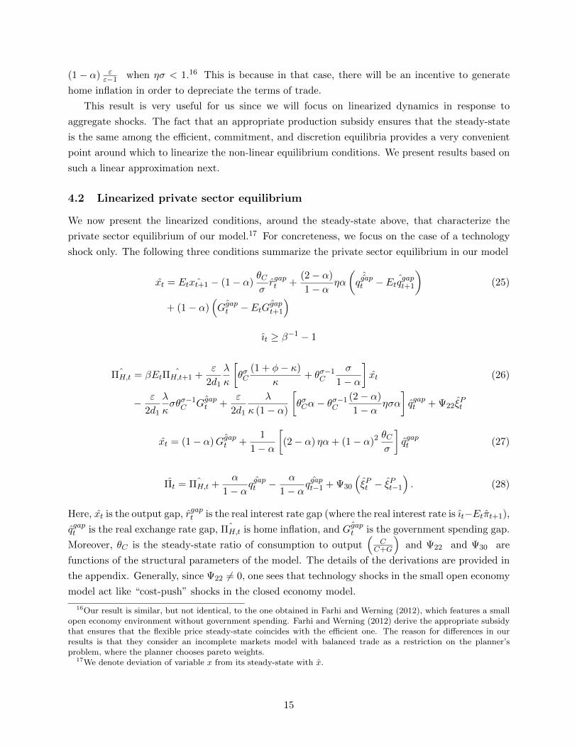
4.2 Linearized private sector equilibrium

We now present the linearized conditions, around the steady-state above, that characterize the

private sector equilibrium of our model.17 For concreteness, we focus on the case of a technology

shock only. The following three conditions summarize the private sector equilibrium in our model

xt = Et ˆxt+1 − (1− α)θCσrgapt +

(2− α)

1− αηα

(ˆqgapt − ˆEtq

gapt+1

)(25)

+ (1− α)(

ˆGgapt − Et ˆGgapt+1

)ıt ≥ β−1 − 1

ˆΠH,t = βEt ˆΠH,t+1 +ε

2d1

λ

κ

[θσC

(1 + φ− κ)

κ+ θσ−1

C

σ

1− α

]xt (26)

− ε

2d1

λ

κσθσ−1

CˆGgapt +

ε

2d1

λ

κ (1− α)

[θσCα− θσ−1

C

(2− α)

1− αησα

]qgapt + Ψ22ξ

Pt

xt = (1− α) ˆGgapt +1

1− α

[(2− α) ηα+ (1− α)2 θC

σ

]qgapt (27)

Πt = ˆΠH,t +α

1− αˆqgapt − α

1− αˆqgapt−1 + Ψ30

(ξPt − ξPt−1

). (28)

Here, xt is the output gap, rgapt is the real interest rate gap (where the real interest rate is ıt−Etπt+1),

qgapt is the real exchange rate gap, ˆΠH,t is home inflation, and ˆGgapt is the government spending gap.

Moreover, θC is the steady-state ratio of consumption to output(

CC+G

)and Ψ22 and Ψ30 are

functions of the structural parameters of the model. The details of the derivations are provided in

the appendix. Generally, since Ψ22 6= 0, one sees that technology shocks in the small open economy

model act like “cost-push” shocks in the closed economy model.

16Our result is similar, but not identical, to the one obtained in Farhi and Werning (2012), which features a smallopen economy environment without government spending. Farhi and Werning (2012) derive the appropriate subsidythat ensures that the flexible price steady-state coincides with the efficient one. The reason for differences in ourresults is that they consider an incomplete markets model with balanced trade as a restriction on the planner’sproblem, where the planner chooses pareto weights.

17We denote deviation of variable x from its steady-state with x.

15

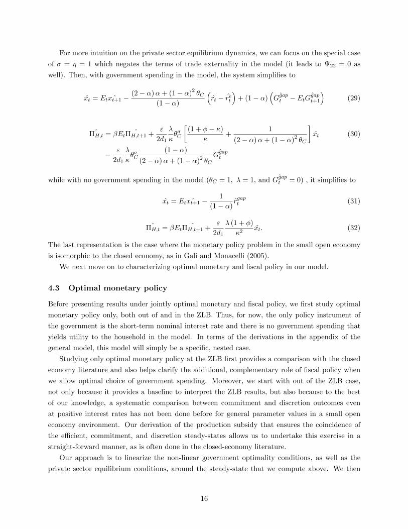
For more intuition on the private sector equilibrium dynamics, we can focus on the special case

of σ = η = 1 which negates the terms of trade externality in the model (it leads to Ψ22 = 0 as

well). Then, with government spending in the model, the system simplifies to

xt = Et ˆxt+1 −(2− α)α+ (1− α)2 θC

(1− α)

(rt − ret

)+ (1− α)

(ˆGgapt − Et ˆGgapt+1

)(29)

ˆΠH,t = βEt ˆΠH,t+1 +ε

2d1

λ

κθσC

[(1 + φ− κ)

κ+

1

(2− α)α+ (1− α)2 θC

]xt (30)

− ε

2d1

λ

κθσC

(1− α)

(2− α)α+ (1− α)2 θC

ˆGgapt

while with no government spending in the model (θC = 1, λ = 1, and ˆGgapt = 0) , it simplifies to

xt = Et ˆxt+1 −1

(1− α)rgapt (31)

ˆΠH,t = βEt ˆΠH,t+1 +ε

2d1

λ (1 + φ)

κ2xt. (32)

The last representation is the case where the monetary policy problem in the small open economy

is isomorphic to the closed economy, as in Gali and Monacelli (2005).

We next move on to characterizing optimal monetary and fiscal policy in our model.

4.3 Optimal monetary policy

Before presenting results under jointly optimal monetary and fiscal policy, we first study optimal

monetary policy only, both out of and in the ZLB. Thus, for now, the only policy instrument of

the government is the short-term nominal interest rate and there is no government spending that

yields utility to the household in the model. In terms of the derivations in the appendix of the

general model, this model will simply be a specific, nested case.

Studying only optimal monetary policy at the ZLB first provides a comparison with the closed

economy literature and also helps clarify the additional, complementary role of fiscal policy when

we allow optimal choice of government spending. Moreover, we start with out of the ZLB case,

not only because it provides a baseline to interpret the ZLB results, but also because to the best

of our knowledge, a systematic comparison between commitment and discretion outcomes even

at positive interest rates has not been done before for general parameter values in a small open

economy environment. Our derivation of the production subsidy that ensures the coincidence of

the efficient, commitment, and discretion steady-states allows us to undertake this exercise in a

straight-forward manner, as is often done in the closed-economy literature.

Our approach is to linearize the non-linear government optimality conditions, as well as the

private sector equilibrium conditions, around the steady-state that we compute above. We then

16

study the dynamics of the model in the neighborhood of the steady-state when an unexpected

shock hits the economy. For the commitment case, as is well-known, generally there exists a

time-inconsistency feature of the equilibrium. In particular, the period 0 government optimality

conditions are different from period 1 onwards. As in Khan, King, and Wolman (1999), the nu-

merical results we present are based on setting the initial lagrange multipliers that appear in the

government optimality conditions to their steady-state values.

We rely on numerical results since analytical results are not available except for the special case

of σ = η = 1 when the ZLB does not bind.18 Our calibration is very standard and we present

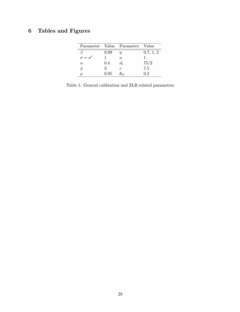
the parameter values we use in Table 1. For most parts, we use the same parameter values as in

Faia and Monacelli (2008), including log-utility (σ = 1), constant returns to scale in production

(κ = 1) , and trade openness (α = 0.4). To conserve space, we then mostly focus on showing results

for different values of η, the elasticity of substitution between between domestic and foreign goods,

since there is disagreement in the literature regarding a reasonable estimate of this parameter.

We have however, undertaken robustness exercises with respect to the intertemporal elasticity of

substitution, as well as, trade openness. The scale parameter in the utility function, λ, is chosen

so that the steady-state is consistent with our normalization that steady-state output is 1.

Moreover, to conserve space, we focus on technology shocks since that is often the baseline

case analyzed in the optimal monetary policy literature. We consider a persistent process with an

AR(1) parameter (ρ) of 0.95. The ZLB case then arises when a one-time large enough technology

shock hits the economy initially. The model then evolves deterministically after the shock is over

and eventually, the economy exits from the liquidity trap. Our results on when we consider a large

negative preference shock that drives the economy into the liquidity trap are qualitatively the same.

For the computation of the ZLB case, we use the piece-wise linear algorithm developed by Jung,

Teranishi, Watanabe (2005), to which we refer the reader for details. We also briefly describe the

algorithm in the appendix.19

4.3.1 Out of ZLB

We start with the case where a positive technology shock hits the economy and the shock is not

big enough to drive the economy into a liquidity trap. We first consider when the government can

commit and then move on to the discretion case.

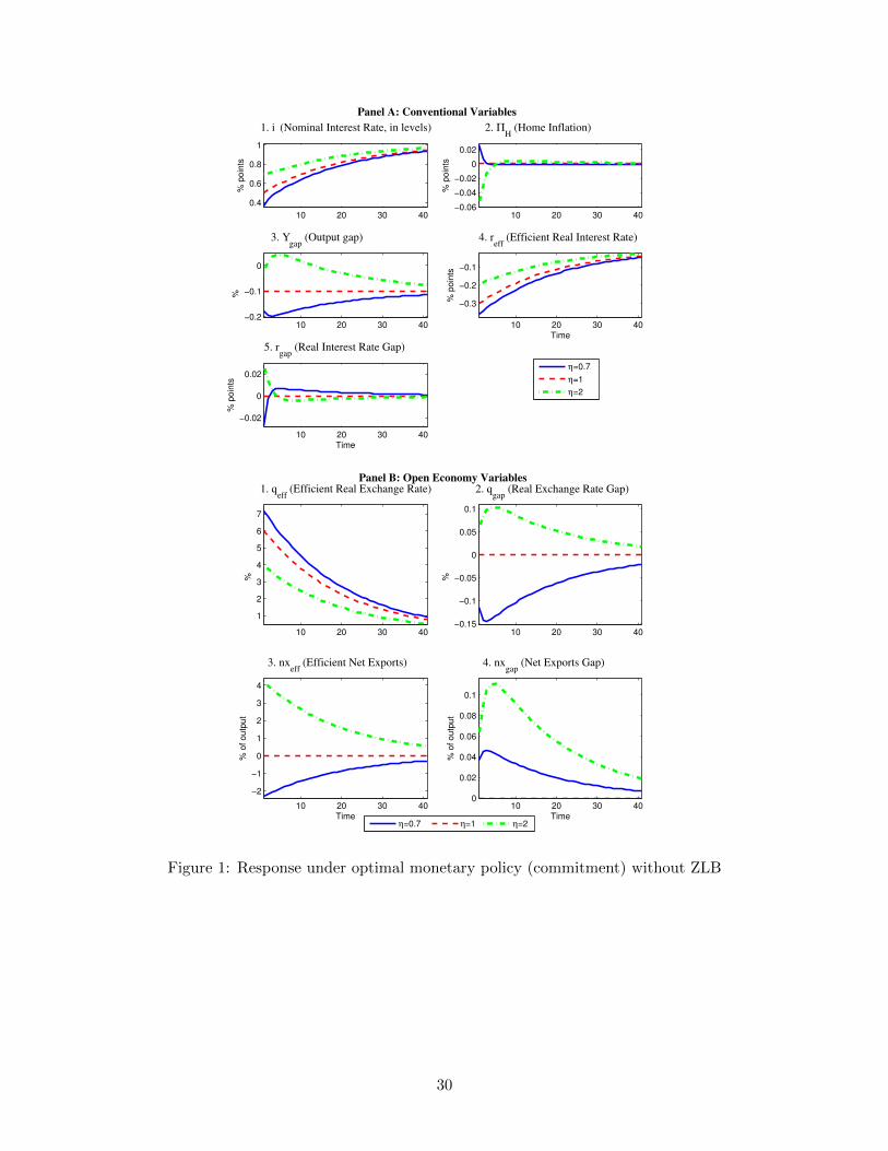
Commitment Figure 1 shows the dynamic response of various model variables under optimal

monetary policy with commitment at different value of η, the elasticity of substitution between

18This is the case analyzed in Gali and Monacelli (2005), under which the open economy policy problem is isomor-phic to the closed economy one; a simple linear quadratic approach to optimal policy is valid; and, finally, monetarypolicy achieves first best with technology shocks.

19In modelling the binding ZLB as arising in a perfect foresight environment due to an unexpected, one-time shockthat drives the efficient real interest to a large negative value, we follow, among others, Jung, Teranishi, Watanabe(2005), Christiano, Eichenbaum, and Rebelo (2011), and Werning (2013).We use the Dynare based Occbin toolboxfor our computations.

17

between domestic and foreign goods.20 Panel (a) shows the responses of conventional variables.

Focussing first on η = 1 (note that we have already imposed σ = 1), it is clear that the policy

problem is isomorphic to the closed economy as it entails setting output gap and producer (home)

inflation to zero. Panel (b) shows the responses of open economy variables. Again, focussing

first on η = 1 and combining with results from panel (a), it is clear that optimal policy achieves

the efficient outcome as the real exchange rate gap and the next exports gap are both zero. In

addition, in this special case, both the efficient and the actual level of net exports is zero: the

economy with and without frictions features balanced trade. These results follow the analysis of

Gali and Monacelli (2005) as the models are the same substantively and while we follow a non-

linear approach to optimal policy, the linear-quadratic approach of Gali and Monacelli (2005) is

equivalent under σ = η = 1 We can formally state this result.

Proposition 2 As in Gali and Monacelli (2005), under log-utility and unit elasticity of substitution

between domestic and foreign goods (σ = η = 1), at positive interest rates, optimal monetary policy

with commitment achieves the efficient outcome by setting home-inflation and output gap to zero.

Proof. In appendix.

Moreover, regardless of the value of η, as to be expected, the nominal interest rate and the

efficient real interest rate decline while the efficient level of the real exchange rate depreciates when

a positive productivity shock perturbs the economy.21 Generally, however, as also emphasized in

Faia and Monacelli (2008), the first-best is not achieved. The central bank now faces a dynamic

trade-off between its stabilization objectives. In particular, the real exchange rate now deviates

from its efficient level. Moreover, note that the output gap and home inflation move in opposite

direction initially, similar to the response under a “markup” shock in the closed economy case. Thus,

technology shocks acts like an endogenous mark-up/trade-off shock in this general environment, as

we also emphasized in discussing (26) above.22

As is intuitive, the real interest rate gap and the real exchange rate gap is higher, lower is

the elasticity of substitution between domestic and foreign goods as now (relative) prices have to

adjust more to clear the goods market. Finally, whether the output gap, home inflation, and the

real exchange rate gap are affected positively or negatively depends crucially on the trade elasticity.

Net exports gap however, is always positive.

Discretion Figure 2 shows the dynamic response of various model variables under optimal mon-

etary policy without commitment at different value of η, the elasticity of substitution between

domestic and foreign goods. Again, focussing first on η = 1 (note that we have already imposed

20Throughout, we consider a shock of size 0.1 for the out of ZLB case.21What we mean by the efficient real interest rate is the real interest rate that is consistent with consumption being

at the efficient level (and is backed out from a hypothetical consumption euler equation). This is a counterfactualnotion.

22This is similar to the result in extended versions of the simple closed economy sticky price model, say undereither wage stickiness or in a two sector sticky price model, where technology shocks greate a trade-off betweenseveral objectives and act like a markup shock in a one-sector model.

18

σ = 1), it is clear from panel (a) that the policy problem is isomorphic to the closed economy as

it entails setting output gap and producer (home) inflation to zero. Moreover, combining this with

panel (b), it is clear that this also achieves the efficient outcome as the real exchange rate gap and

the next exports gap are both zero. Thus, in this special case, like in the closed-economy, there is

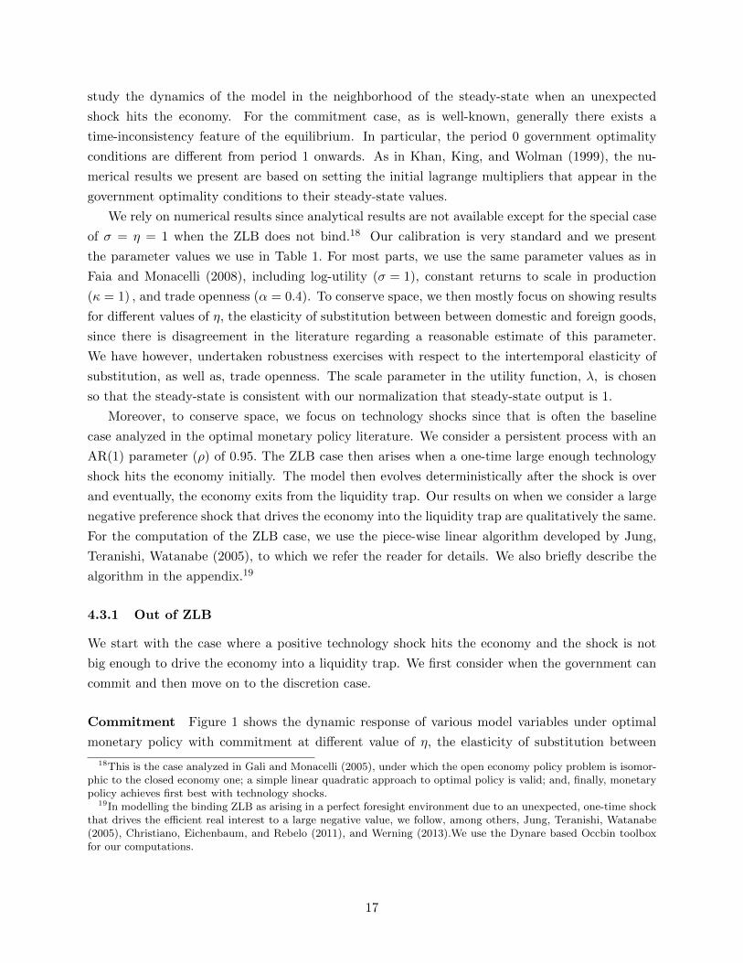
no difference between the commitment and discretion outcomes. We can formally state this result.

Proposition 3 Under log-utility and unit elasticity of substitution between domestic and foreign

goods (σ = η = 1), at positive interest rates, optimal monetary policy without commitment achieves

the efficient outcome by setting home-inflation and output gap to zero. There is thus no difference

between the commitment and discretion outcomes.

Proof. In appendix.

Generally though, the first-best is not achieved and there is a difference between when the

central bank can and when it cannot commit to future actions. As is intuitive, it is clear that the

outcomes are generally worse (in terms of deviations of variables from their efficient levels) under

discretion compared to commitment. At the same time though, this implies that the commitment

outcome is time inconsistent: the central bank has incentives to renege on its promises in future.

In order to highlight the differences between commitment and discretion, we show in Figure

3 the responses under η = 0.7 for an iid shock. This case is useful because it highlights how under

commitment, there is “history dependence” of outcomes even without persistence of shock.23 In

particular, note that the discretion problem reduces to a period-by-period maximization in our

model. As is clear, when the central bank is able to promise to a state contingent future path, it

improves current outcomes as inflation, output gap, real exchange rate gap, and net exports gap

get affected by less on the period when the shock hits. Thus, discretion suffers from a “stabilization

bias,”a feature of forward looking models when the central bank faces a dynamic trade-off between

several variables: the economy responds strongly during the current period and then reverts back

to steady-state the period after.

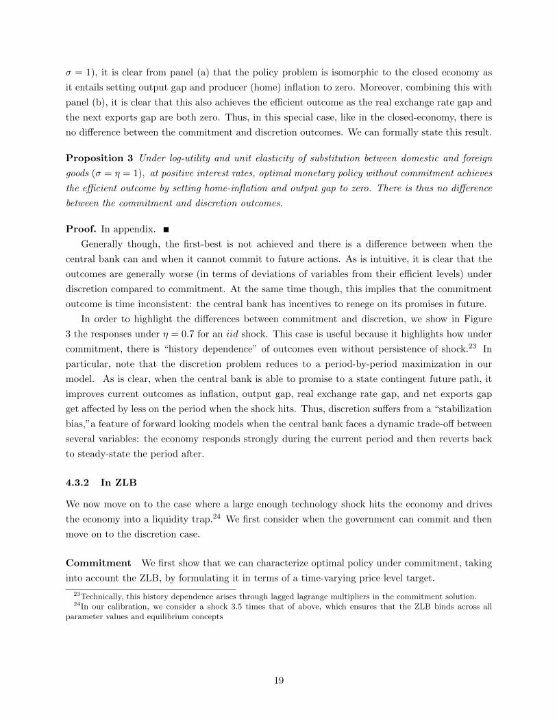
4.3.2 In ZLB

We now move on to the case where a large enough technology shock hits the economy and drives

the economy into a liquidity trap.24 We first consider when the government can commit and then

move on to the discretion case.

Commitment We first show that we can characterize optimal policy under commitment, taking

into account the ZLB, by formulating it in terms of a time-varying price level target.

23Technically, this history dependence arises through lagged lagrange multipliers in the commitment solution.24In our calibration, we consider a shock 3.5 times that of above, which ensures that the ZLB binds across all

parameter values and equilibrium concepts

19

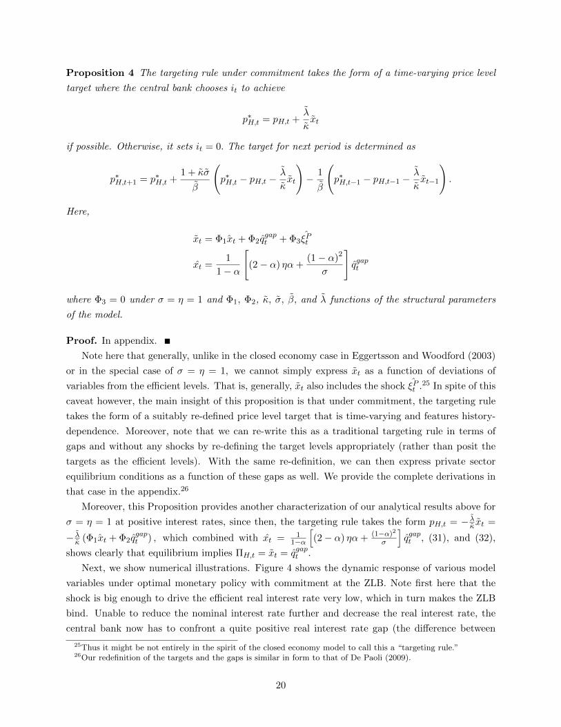
Proposition 4 The targeting rule under commitment takes the form of a time-varying price level

target where the central bank chooses it to achieve

p∗H,t = pH,t +λ

κxt

if possible. Otherwise, it sets it = 0. The target for next period is determined as

p∗H,t+1 = p∗H,t +1 + κσ

β

(p∗H,t − pH,t −

λ

κxt

)− 1

β

(p∗H,t−1 − pH,t−1 −

λ

κxt−1

).

Here,

xt = Φ ˆ1xt + Φ2qgapt + Φ3ξPt

xt =1

1− α

[(2− α) ηα+

(1− α)2

σ

]qgapt

where Φ3 = 0 under σ = η = 1 and Φ1, Φ2, κ, σ, β, and λ functions of the structural parameters

of the model.

Proof. In appendix.

Note here that generally, unlike in the closed economy case in Eggertsson and Woodford (2003)

or in the special case of σ = η = 1, we cannot simply express xt as a function of deviations of

variables from the efficient levels. That is, generally, xt also includes the shock ξPt .25 In spite of this

caveat however, the main insight of this proposition is that under commitment, the targeting rule

takes the form of a suitably re-defined price level target that is time-varying and features history-

dependence. Moreover, note that we can re-write this as a traditional targeting rule in terms of

gaps and without any shocks by re-defining the target levels appropriately (rather than posit the

targets as the efficient levels). With the same re-definition, we can then express private sector

equilibrium conditions as a function of these gaps as well. We provide the complete derivations in

that case in the appendix.26

Moreover, this Proposition provides another characterization of our analytical results above for

σ = η = 1 at positive interest rates, since then, the targeting rule takes the form pH,t = − λκ xt =

− λκ (Φ ˆ1xt + Φ2q

gapt ) , which combined with xt = 1

1−α

[(2− α) ηα+ (1−α)2

σ

]qgapt , (31), and (32),

shows clearly that equilibrium implies ΠH,t = xt = qgapt .

Next, we show numerical illustrations. Figure 4 shows the dynamic response of various model

variables under optimal monetary policy with commitment at the ZLB. Note first here that the

shock is big enough to drive the efficient real interest rate very low, which in turn makes the ZLB

bind. Unable to reduce the nominal interest rate further and decrease the real interest rate, the

central bank now has to confront a quite positive real interest rate gap (the difference between

25Thus it might be not entirely in the spirit of the closed economy model to call this a “targeting rule.”26Our redefinition of the targets and the gaps is similar in form to that of De Paoli (2009).

20

the real interest rate and its efficient level). As is standard in the closed economy literature and

shown in panel (a), the equilibrium thereby features a negative output gap and producer price

(home) deflation initially. Moreover, now in an open economy, the ZLB also leads to a positive

real exchange rate gap as shown in panel (b): the real exchange rate is appreciated compared to

its efficient level.

The extent of these adverse effects and the duration of the liquidity trap is higher, lower is

the elasticity of substitution between domestic and foreign goods. This is so because when the

elasticity of substitution between domestic and foreign goods is lower, equilibrium requires a higher

response of relative prices to clear the goods market. In a liquidity trap situation, since the price

adjustment channel gets severely impaired, this implies that the economy suffers from a bigger

output gap, producer price deflation, and a real exchange rate gap. As a result of these adverse

effects, optimal monetary policy, keeps nominal interest rates at zero for longer when the elasticity

of substitution between domestic and foreign goods is lower.27 Thus, the duration of liquidity trap

depends importantly on the trade elasticity in a small open economy.

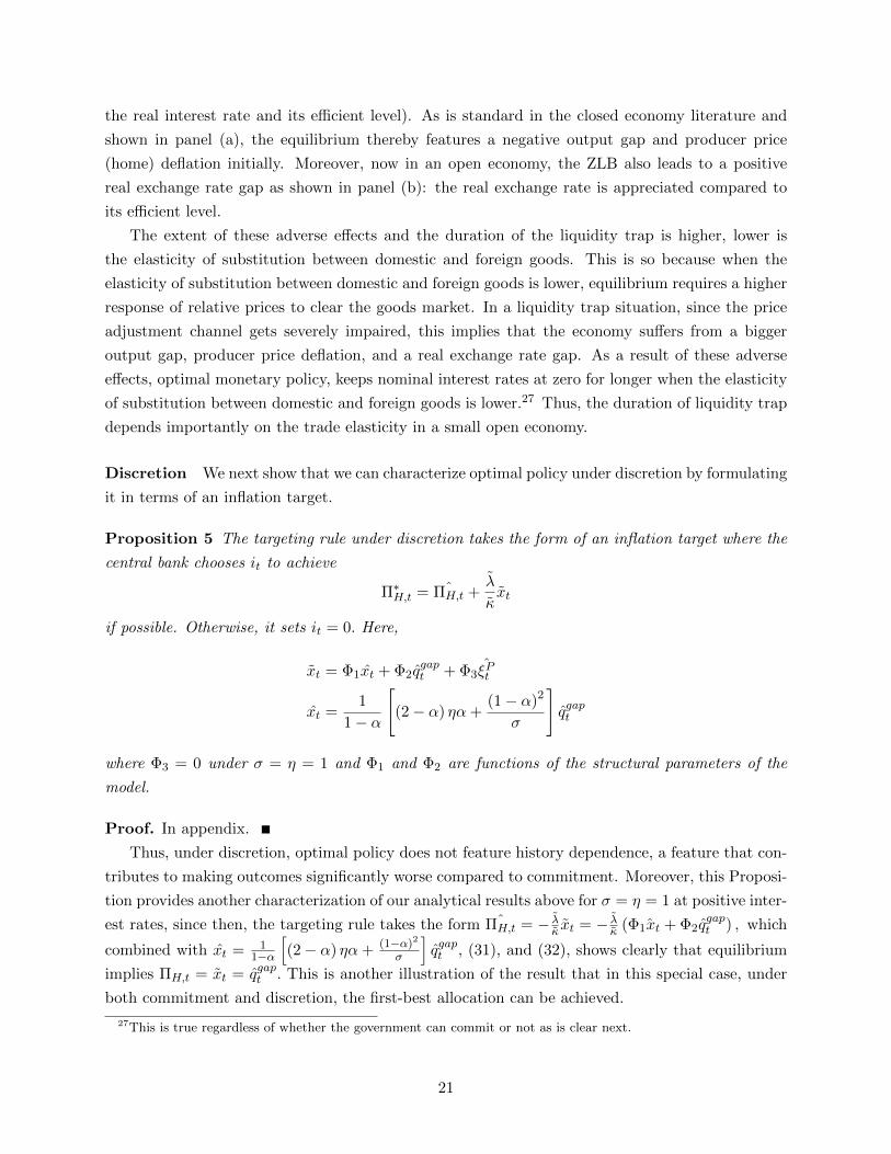
Discretion We next show that we can characterize optimal policy under discretion by formulating

it in terms of an inflation target.

Proposition 5 The targeting rule under discretion takes the form of an inflation target where the

central bank chooses it to achieve

Π∗H,t = ˆΠH,t +λ

κxt

if possible. Otherwise, it sets it = 0. Here,

xt = Φ1xt + Φ2qgapt + Φ3ξPt

xt =1

1− α

[(2− α) ηα+

(1− α)2

σ

]qgapt

where Φ3 = 0 under σ = η = 1 and Φ1 and Φ2 are functions of the structural parameters of the

model.

Proof. In appendix.

Thus, under discretion, optimal policy does not feature history dependence, a feature that con-

tributes to making outcomes significantly worse compared to commitment. Moreover, this Proposi-

tion provides another characterization of our analytical results above for σ = η = 1 at positive inter-

est rates, since then, the targeting rule takes the form ˆΠH,t = − λκ xt = − λ

κ (Φ ˆ1xt + Φ2qgapt ) , which

combined with xt = 11−α

[(2− α) ηα+ (1−α)2

σ

]qgapt , (31), and (32), shows clearly that equilibrium

implies ΠH,t = xt = qgapt . This is another illustration of the result that in this special case, under

both commitment and discretion, the first-best allocation can be achieved.

27This is true regardless of whether the government can commit or not as is clear next.

21

Figure 5 shows the dynamic response of various model variables under optimal monetary policy

without commitment at the ZLB. First note that like under commitment, the extent of adverse

effects during a liquidity trap are higher, lower is the elasticity of substitution between domestic

and foreign goods. Next, several results stand out when compared to commitment. The equilibrium

under commitment, compared to discretion, features a less severe negative output gap and producer

price deflation, as shown clearly by comparing panel (a)s of the two Figures. Thus, the usual

“deflation bias”of discretionary policy at zero interest rates that is present in a closed economy is

also a feature of the small open economy. In particular, under commitment, the central bank is

able to promise low real interest rates and a higher output gap in future, which helps mitigate the

extent of the negative output gap during the initial periods. As part of the equilibrium, optimal

commitment policy involves an increase in home inflation in later periods as well

In a small open economy environment, there is in addition, also a “overvaluation bias” associated

with discretionary policy: the real exchange rate is relatively more appreciated. This can be seen

clearly by comparing panel (b)s of the two Figures. Thus, under optimal policy under commitment,

the central bank promises a more depreciated real exchange rate. Contrary to what might appear

intuitive however, whether the net exports gap is more negative under discretion compared to

commitment depends on the trade elasticity. Thus, it is generally not true that if possible, a

discretionary central bank at the ZLB would like to commit to a higher level of net exports in

future.

In order to highlight the differences between commitment and discretion, like before, we show in

Figure 6 the responses under η = 0.7 for an iid shock. This comparison is particularly informative

since now the duration of zero nominal interest rates is simply one period for the discretion case.

The usual “deflation bias” (panel (a)) and the new “overvaluation bias” (panel (b)) of discretionary

monetary policy in a liquidity trap are now especially clear. In particular, under commitment, the

central bank promises a future low real interest rate gap and associated with it, a less negative

output gap, higher inflation, and a more depreciated real exchange rate. In this parameterization,

this is achieved by keeping the nominal interest rate at zero for several additional periods after the

shock is over.

4.4 Optimal monetary and fiscal policy

We now move on to considering joint conduct of optimal monetary and fiscal policy. The policy

instruments of the government are now the short-term nominal interest rate and the level of public

spending. As given in Table 1, we choose the steady-state government spending-to-output ratio,

θG, of 0.2. The scale parameter in the utility function, λG, is then chosen so that the steady-state

of the model is consistent with this choice.

One of the main motivations for this extension is that while the commitment outcome under

optimal monetary policy is superior to discretion, it suffers from dynamic time inconsistency: the

central bank has incentives to renege on its promises in future. This manifests itself at the ZLB

via a much larger negative output gap, producer price deflation, and an appreciated real exchange

22

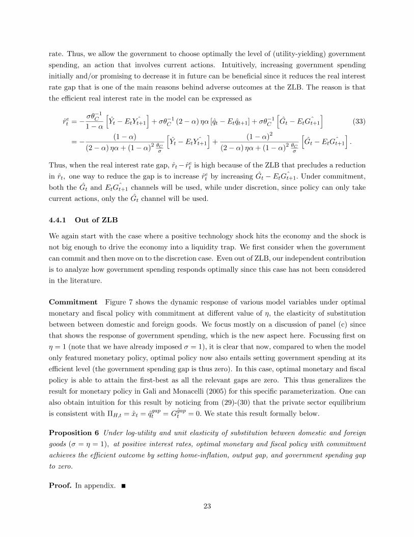
rate. Thus, we allow the government to choose optimally the level of (utility-yielding) government

spending, an action that involves current actions. Intuitively, increasing government spending

initially and/or promising to decrease it in future can be beneficial since it reduces the real interest

rate gap that is one of the main reasons behind adverse outcomes at the ZLB. The reason is that

the efficient real interest rate in the model can be expressed as

ret = −σθ−1

C

1− α

[Yt − Et ˆYt+1

]+ σθ−1

C (2− α) ηα [qt − Etqt+1] + σθ−1C

[Gt − Et ˆGt+1

](33)

= − (1− α)

(2− α) ηα+ (1− α)2 θCσ

[Yt − Et ˆYt+1

]+

(1− α)2

(2− α) ηα+ (1− α)2 θCσ

[Gt − Et ˆGt+1

].

Thus, when the real interest rate gap, rt− ret is high because of the ZLB that precludes a reduction

in rt, one way to reduce the gap is to increase ret by increasing Gt − Et ˆGt+1. Under commitment,

both the Gt and Et ˆGt+1 channels will be used, while under discretion, since policy can only take

current actions, only the Gt channel will be used.

4.4.1 Out of ZLB

We again start with the case where a positive technology shock hits the economy and the shock is

not big enough to drive the economy into a liquidity trap. We first consider when the government

can commit and then move on to the discretion case. Even out of ZLB, our independent contribution

is to analyze how government spending responds optimally since this case has not been considered

in the literature.

Commitment Figure 7 shows the dynamic response of various model variables under optimal

monetary and fiscal policy with commitment at different value of η, the elasticity of substitution

between between domestic and foreign goods. We focus mostly on a discussion of panel (c) since

that shows the response of government spending, which is the new aspect here. Focussing first on

η = 1 (note that we have already imposed σ = 1), it is clear that now, compared to when the model

only featured monetary policy, optimal policy now also entails setting government spending at its

efficient level (the government spending gap is thus zero). In this case, optimal monetary and fiscal

policy is able to attain the first-best as all the relevant gaps are zero. This thus generalizes the

result for monetary policy in Gali and Monacelli (2005) for this specific parameterization. One can

also obtain intuition for this result by noticing from (29)-(30) that the private sector equilibrium

is consistent with ΠH,t = xt = qgapt = ˆGgapt = 0. We state this result formally below.

Proposition 6 Under log-utility and unit elasticity of substitution between domestic and foreign

goods (σ = η = 1), at positive interest rates, optimal monetary and fiscal policy with commitment

achieves the efficient outcome by setting home-inflation, output gap, and government spending gap

to zero.

Proof. In appendix.

23

Generally, for any value of η however, the first-best is not achieved. In particular, generally,

it is optimal to let government spending to deviate from its efficient level. Whether government

spending increases or decreases compared to the efficient level however, depends crucially on the

trade elasticity. In particular, the government spending gap is positive for low values of η. Overall,

regardless of a positive or negative government spending gap, optimal fiscal policy leads to a smaller

real interest rate gap compared to only optimal monetary policy. This in turn lead to a lower effect

on output gap, home inflation, and real exchange rate gap. There is thus an independent and

complementary role for government spending even at positive interest rates in a general small open

economy environment.

Discretion Figure 8 shows the dynamic response of various model variables under optimal mon-

etary and fiscal policy without commitment at different value of η, the elasticity of substitution

between domestic and foreign goods. Focussing on panel (c) and first on η = 1 (note that we have

already imposed σ = 1), it is clear that now, compared to when the model only featured monetary

policy, optimal policy now also entails setting government spending at its efficient level (the gov-

ernment spending gap is thus zero). In this case, optimal monetary and fiscal policy is again able

to attain the first-best and there is no difference between the commitment and discretion outcomes.

We state this result formally below.

Proposition 7 Under log-utility and unit elasticity of substitution between domestic and foreign

goods (σ = η = 1), at positive interest rates, optimal monetary and fiscal policy without commitment

achieves the efficient outcome by setting home-inflation, output gap, and government spending gap

to zero. There is thus no difference between the commitment and discretion outcomes.

Proof. In appendix.

Generally though, the first-best is not achieved and there is a difference between when the

central bank can and when it cannot commit to future actions. As is intuitive, it is clear that the

outcomes are worse (in terms of deviations of variables from their efficient levels) under discretion

compared to commitment. The most interesting comparison between the two cases is how the path

of government spending gap is different: under commitment, there is a hump-shaped response that

is absent under discretion. This is because under commitment, the government can affect the real

interest rate gap by both current-period actions as well as those in future periods. In contrast,

under discretion, since the maximization problem is period-by-period, the responses of government

spending simply follow the persistence of the shock.

4.4.2 In ZLB

We now move on to the case where a large enough technology shock hits the economy and drives

the economy into a liquidity trap. We first consider when the government can commit and then

move on to the discretion case.

24

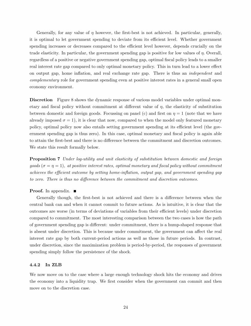
Commitment Figure 9 shows the dynamic response of various model variables under optimal

monetary and fiscal policy with commitment at the ZLB. We focus on discussing the dynamics of

government spending in panel (c) since that is new now compared to before. As is clear, optimal

fiscal policy entails a positive government expenditure gap for several periods initially, which then

reverses to a negative output gap eventually. Comparing with the dynamics of output gap, then

it is clear that optimal fiscal policy entails countercyclical government spending. This response is

optimal because by both increasing government spending initially, and then promising to decrease

it in future once the economy has recovered, the government is able to reduce the real interest rate

gap during the liquidity trap. This is clear from the expression for the efficient real interest rate in

(33). This then improves outcomes at the ZLB with respect to negative output gap, deflation, and

the real exchange rate gap.28

The extent of the optimal increase in government spending beyond the efficient level decreases

when the elasticity of substitution between domestic and foreign goods is higher. This is because the

increase in government spending generates real exchange rate appreciation, which reduces welfare

more when the elasticity of substitution between domestic and foreign goods is higher. This is true

both under commitment as well as discretion, which we discuss next.

Discretion Figure 10 shows the dynamic response of various model variables under optimal

monetary policy without commitment at the ZLB. Again, we focus on discussing the dynamics of

government spending since that is new now compared to before. Note that now under discretion,

government spending increases by more initially compared to commitment. In particular, govern-

ment spending gap does not go negative in later periods, unlike commitment. The reason is that

now since the government cannot commit, to achieve its goal of decreasing the real interest rate

gap, it cannot promise a negative government spending gap in future. Thus, it solely has to rely on

a higher level of government spending today. Even then however, this additional policy tool allows

it to improve outcomes on output gap, deflation, and real exchange rate gap, all of which now are

affected less compared to when we considered only discretionary monetary policy.

5 Conclusion

In this paper, we studied optimal monetary and fiscal policy at zero nominal interest rates, both

with and without commitment, in a small open economy with sticky prices. In such a liquidity

trap situation, the economy suffers from a negative output gap, producer price deflation, and an

appreciated real exchange rate (compared to its efficient level). The extent of these adverse effects

and the duration of the liquidity trap is higher, lower is the elasticity of substitution of between

domestic and foreign goods. Under discretion, compared to commitment, in addition to the usual

“deflation bias” present in a closed economy, the equilibrium in a small open economy also features

an “overvaluation bias”: the real exchange rate is excessively appreciated compared to its efficient

28Note however that while the government spending gap is positive initially always, whether the level of governmentspending increases or decreases depends on the trade elasticity.

25

level. Countercyclical fiscal policy, that is, increasing government spending above the efficient

level during the liquidity trap, constitutes optimal policy and helps decrease the extent of negative

output gap and deflation, especially under discretion, but the extent of the increase in government

spending is lower when the elasticity of substitution of between domestic and foreign goods is

higher.

In future work, we can extend our work in both theoretical and quantitative directions. First,

while we have only considered optimal government spending policy, in closed economy models,

Eggertsson and Woodford (2006) and Correia et al (2013) have shown that with enough tax in-

struments, fiscal policy can achieve the first-best even at the ZLB. It will be interesting to do a

similar exercise in our small open economy set-up and our result on the nature of the appropriate

production subsidy that ensures that the steady-state is efficient can help guide us. Second, we

have considered a model where there is perfect risk-sharing between the small open economy and

the rest of the world. Relaxing this assumption by considering incomplete markets would provide

additional role for real exchange rate and trade imbalances in driving optimal policy decisions.

Finally, to evaluate more thoroughly the quantitative predictions of our model, we can consider

a set-up that features more frictions such as sticky wages and pricing to market/local currency

pricing.

References

[1] Adam, Klaus, and Roberto Billi (2006), “Optimal Monetary Policy under Commitment with

a Zero Bound on Nominal Interest Rates,” Journal of Money, Credit, and Banking, 38, 1877-

1905.

[2] Adam, Klaus, and Roberto Billi (2007), “Discretionary Monetary Policy and the Zero Lower

Bound on Nominal Interest Rates,” Journal of Monetary Economics, 54, 728-752.

[3] Benigno, Gianluca, and Pierpaolo Benigno (2003), “Price Stability in Open Economies,” Re-

view of Economic Studies, 70, 743-764.

[4] Benigno, Pierpaolo, and Michael Woodford (2012), “Linear-Quadratic Approximation of Op-

timal Policy Problems,” Journal of Economic Theory, 147, 1-42.

[5] Bodenstein, Martin, Christopher J. Erceg, and Luca Guerrieri (2009), “The Effects of Foreign

Shocks When Interest Rates are at Zero,” working paper.

[6] Cook, David, and Michael B. Devereux (2013), “Sharing the Burden: Monetary and Fiscal

Responses to a World Liquidity Trap,” American Economic Journal: Macroeconomics, 5, 190-

228.

[7] Correia, Isabel, Emmanuel Farhi, Juan Pablo Nicolini, and Pedro Teles (2013), “Unconven-

tional Fiscal Policy at the Zero Bound,” American Economic Review, 103, 1172-1211.

26

[8] Christiano, Lawrence, Martin Eichenbaum, and Sergio Rebelo (2011), “When Is the Govern-

ment Spending Multiplier Large?” Journal of Political Economy, 119, 78-121.

[9] De Paoli, Bianca (2009), “Monetary Policy and Welfare in a Small Open Economy,” Journal

of International Economics, 77, 11-22.

[10] Eggertsson, Gauti B. (2001), “Real Government Spending in a Liquidity Trap,” working paper.

[11] Eggertsson, Gauti B. (2006), “The Deflation Bias and Committing to Being Irresponsible,”

Journal of Money, Credit, and Banking, 38, 283-321.

[12] Eggertsson, Gauti B. (2011), “What Fiscal Policy is Effective at Zero Interest Rates,” in NBER

Macroeconomics Annual 2010, Chicago, IL: University of Chicago Press.

[13] Eggertsson, Gauti B., Andrea Ferrero, and Andrea Raffo (2013), “Can Structural Reforms

Help Europe,” forthcoming in Journal of Monetary Economics.

[14] Eggertsson, Gauti B., and Paul Krugman (2012), “Debt, Deleveraging, and the Liquidity Trap:

A Fisher-Minsky-Koo Approach,” Quarterly Journal of Economics, 127, 1469-1513.

[15] Eggertsson, Gauti B., and Michael Woodford (2003), “The Zero Bound on Interest Rates and

Optimal Monetary Policy,” Brookings Papers on Economic Activity, 34, 139-235.

[16] Eggertsson, Gauti B., and Michael Woodford (2006), “Optimal Monetary and Fiscal Policy

in a Liquidity Trap,” in NBER International Seminar on Macroeconomics 2004, Cambridge,

MA: MIT Press.

[17] Erceg, Christopher, and Jesper Linde (2014), “Is There a Fiscal Free Lunch in a Liquidity

Trap,” Journal of European Economic Association, 12, 73-107.

[18] Faia, Ester, and Tommaso Monacelli (2008), “Optimal Monetary Policy in a Small Open

Economy with Home Bias,” Journal of Money, Credit, and Banking, 40, 721-750.

[19] Farhi, Emmanuel, and Ivan Werning (2012), “Dealing with the Trilemma: Optimal Capital

Controls with Fixed Exchange Rates,” working paper.

[20] Gali, Jordi, and Tommaso Monacelli (2005), “Monetary Policy and Exchange Rate Volatility

in a Small Open Economy,” Review of Economic Studies, 72, 707-734.

[21] Jeanne, Olivier (2009), “Global Liquidity Trap,” working paper.

[22] Jeanne, Olivier, and Lars E. O. Svensson (2007), “Credible Commitment to Optimal Escape

From a Liquidity Trap: The Role of the Balance Sheet of an Independent Central Bank,”

American Economic Review, 97, 474–490.

[23] Jung, Taehun, Yuki Teranishi, and Tsutomu Watanabe (2005), “Optimal Monetary Policy at

the Zero-Interest-Rate Bound,” Journal of Money, Credit, and Banking, 37, 813-835.

27

[24] Khan, Aubhik, Robert G. King, and Alexander L. Wolman (2003), “Optimal Monetary Policy,”

Review of Economic Studies, 70, 825-860.

[25] Svensson, Lars E. O. (2003), “Escaping from a Liquidity Trap and Deflation: The Foolproof

Way and Others,” Journal of Economic Perspectives, 17, 145-166.

[26] Svensson, Lars E. O. (2004), “The Magic of the Exchange Rate: Optimal Escape from a

Liquidity Trap in Small and Large Open Economies,” working paper.

[27] Werning, Ivan (2013), “Managing a Liquidity Trap: Monetary and Fiscal Policy,” working

paper.

[28] Wolman, Alexander L. (2005), “Real Implications of the Zero Bound on Nominal Interest

Rates,” Journal of Money, Credit, and Banking, 37, 273-296.

[29] Woodford, Michael (2003), Interest and Prices. Princeton, NJ: Princeton University Press.

[30] Woodford, Michael (2011), “Simple Analytics of the Government Expenditure Multiplier,”

American Economic Journal: Macroeconomics, 3, 1-35.

28

6 Tables and Figures

Parameter Value Parameter Value

β 0.99 η 0.7, 1, 2σ = σ′ 1 κ 1α 0.4 d1 75/2φ 3 ε 7.5ρ 0.95 θG 0.2

Table 1: General calibration and ZLB related parameters

29

10 20 30 40

0.4

0.6

0.8

1

Panel A: Conventional Variables

1. i (Nominal Interest Rate, in levels)

% p

oin

ts

10 20 30 40−0.06

−0.04

−0.02

0

0.02

2. ΠH

(Home Inflation)

% p

oin

ts

10 20 30 40−0.2

−0.1

0

3. Ygap

(Output gap) %

10 20 30 40

−0.3

−0.2

−0.1

Time

4. reff

(Efficient Real Interest Rate)

% p

oin

ts

10 20 30 40

−0.02

0

0.02

Time

5. rgap

(Real Interest Rate Gap)

% p

oin

ts

η=0.7

η=1

η=2

10 20 30 40

1

2

3

4

5

6

7

Panel B: Open Economy Variables1. q

eff (Efficient Real Exchange Rate)

%

10 20 30 40−0.15

−0.1

−0.05

0

0.05

0.1

2. qgap

(Real Exchange Rate Gap)

%

10 20 30 40

−2

−1

0

1

2

3

4

Time

3. nxeff

(Efficient Net Exports)

% o

f outp

ut

10 20 30 40 0

0.02

0.04

0.06

0.08

0.1

Time

4. nxgap

(Net Exports Gap)

% o

f outp

ut

η=0.7 η=1 η=2

Figure 1: Response under optimal monetary policy (commitment) without ZLB

30

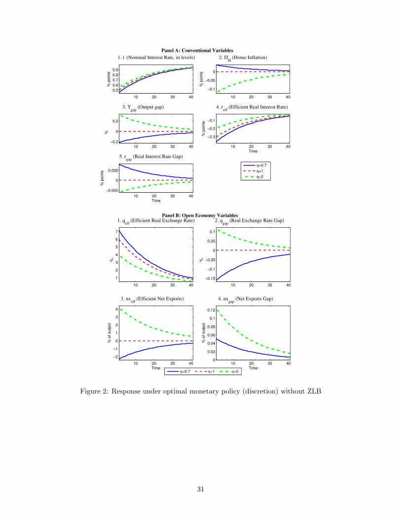
10 20 30 40

0.5

0.6

0.7

0.8

0.9

Panel A: Conventional Variables

1. i (Nominal Interest Rate, in levels)

% p

oin

ts

10 20 30 40

−0.1

−0.05

0

2. ΠH

(Home Inflation)

% p

oin

ts

10 20 30 40−0.2

0

0.2

3. Ygap

(Output gap) %

10 20 30 40

−0.3

−0.2

−0.1

Time

4. reff

(Efficient Real Interest Rate)

% p

oin

ts

10 20 30 40

−0.005

0

0.005

Time

5. rgap

(Real Interest Rate Gap)

% p

oin

ts

η=0.7

η=1

η=2

10 20 30 40

1

2

3

4

5

6

7

Panel B: Open Economy Variables1. q

eff (Efficient Real Exchange Rate)

%

10 20 30 40

−0.15

−0.1

−0.05

0

0.05

0.1

2. qgap

(Real Exchange Rate Gap)

%

10 20 30 40

−2

−1

0

1

2

3

4

Time

3. nxeff

(Efficient Net Exports)

% o

f outp

ut

10 20 30 40 0

0.02

0.04

0.06

0.08

0.1

0.12

Time

4. nxgap

(Net Exports Gap)

% o

f outp

ut

η=0.7 η=1 η=2

Figure 2: Response under optimal monetary policy (discretion) without ZLB

31

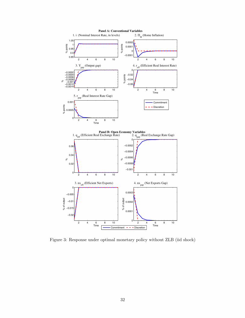
2 4 6 8 100.85

0.9

0.95

1

1.05

Panel A: Conventional Variables

1. i (Nominal Interest Rate, in levels)

% p

oin

ts

2 4 6 8 10

−0.0001

0

0.0001

0.0002

2. ΠH

(Home Inflation)

% p

oin

ts

2 4 6 8 10

−0.0014−0.0012 −0.001

−0.0008−0.0006−0.0004−0.0002

3. Ygap

(Output gap) %

2 4 6 8 10

−0.06

−0.04

−0.02

0

Time

4. reff

(Efficient Real Interest Rate)

% p

oin

ts

2 4 6 8 10 0

0.0005

0.001

Time

5. rgap

(Real Interest Rate Gap)

% p

oin

ts

Commitment

Discretion

2 4 6 8 10 0

0.02

0.04

0.06

Panel B: Open Economy Variables1. q

eff (Efficient Real Exchange Rate)

%

2 4 6 8 10

−0.001

−0.0008

−0.0006

−0.0004

−0.0002

0

2. qgap

(Real Exchange Rate Gap)

%

2 4 6 8 10

−0.02

−0.015

−0.01

−0.005

0

Time

3. nxeff

(Efficient Net Exports)

% o

f outp

ut

2 4 6 8 10 0

0.0001

0.0002

0.0003

Time

4. nxgap

(Net Exports Gap)

% o

f outp

ut

Commitment Discretion

Figure 3: Response under optimal monetary policy without ZLB (iid shock)

32

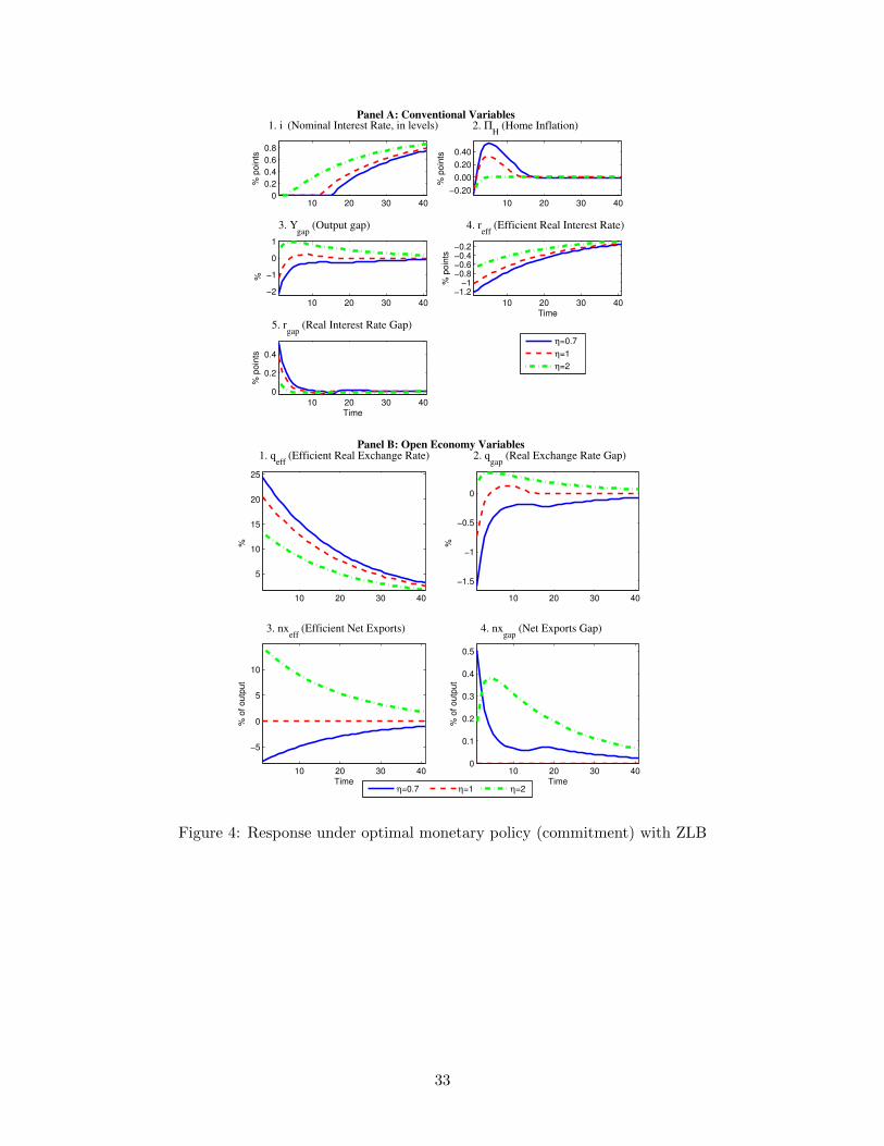
10 20 30 40 0

0.2

0.4

0.6

0.8

Panel A: Conventional Variables

1. i (Nominal Interest Rate, in levels)

% p

oin

ts

10 20 30 40

−0.20

0.00

0.20

0.40

2. ΠH

(Home Inflation)

% p

oin

ts

10 20 30 40

−2

−1

0

1

3. Ygap

(Output gap)

%

10 20 30 40

−1.2 −1−0.8−0.6−0.4−0.2

Time

4. reff

(Efficient Real Interest Rate)

% p

oin

ts

10 20 30 40

0

0.2

0.4

Time

5. rgap

(Real Interest Rate Gap)

% p

oin

ts

η=0.7

η=1

η=2

10 20 30 40

5

10

15

20

25

Panel B: Open Economy Variables1. q

eff (Efficient Real Exchange Rate)

%

10 20 30 40

−1.5

−1

−0.5

0

2. qgap

(Real Exchange Rate Gap) %

10 20 30 40

−5

0

5

10

Time

3. nxeff

(Efficient Net Exports)

% o

f outp

ut

10 20 30 40 0

0.1

0.2

0.3

0.4

0.5

Time

4. nxgap

(Net Exports Gap)

% o

f outp

ut

η=0.7 η=1 η=2

Figure 4: Response under optimal monetary policy (commitment) with ZLB

33

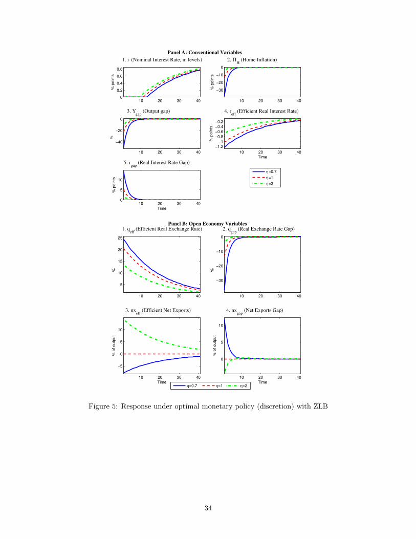
10 20 30 40 0

0.2

0.4

0.6

0.8

Panel A: Conventional Variables

1. i (Nominal Interest Rate, in levels)

% p

oin

ts

10 20 30 40

−30

−20

−10

0

2. ΠH

(Home Inflation)

% p

oin

ts

10 20 30 40

−40

−20

0

3. Ygap

(Output gap) %

10 20 30 40

−1.2

−1

−0.8

−0.6

−0.4

−0.2

Time

4. reff

(Efficient Real Interest Rate)

% p

oin

ts

10 20 30 40 0

5

10

Time

5. rgap

(Real Interest Rate Gap)

% p

oin

ts

η=0.7

η=1

η=2

10 20 30 40

5

10

15

20

25

Panel B: Open Economy Variables1. q

eff (Efficient Real Exchange Rate)

%

10 20 30 40

−30

−20

−10

0

2. qgap

(Real Exchange Rate Gap)

%

10 20 30 40

−5

0

5

10

Time

3. nxeff

(Efficient Net Exports)

% o

f outp

ut

10 20 30 40

0

5

10

Time

4. nxgap

(Net Exports Gap)

% o

f outp

ut

η=0.7 η=1 η=2

Figure 5: Response under optimal monetary policy (discretion) with ZLB

34

2 4 6 8 10 0

0.5

1

Panel A: Conventional Variables

1. i (Nominal Interest Rate, in levels)

% p

oin

ts

2 4 6 8 10

−10

−5

0

5

2. ΠH

(Home Inflation)

% p

oin

ts

2 4 6 8 10

−30

−20

−10

0

3. Ygap

(Output gap) %

2 4 6 8 10−30

−20

−10

0

Time

4. reff

(Efficient Real Interest Rate)

% p

oin

ts

2 4 6 8 10

0

10

20

Time

5. rgap

(Real Interest Rate Gap)

% p

oin

ts

Commitment

Discretion

2 4 6 8 10 0

5

10

15

20

25

30

Panel B: Open Economy Variables1. q

eff (Efficient Real Exchange Rate)

%

2 4 6 8 10

−25

−20

−15

−10

−5

0

5

2. qgap

(Real Exchange Rate Gap)

%

2 4 6 8 10

−8

−6

−4

−2

0

Time

3. nxeff

(Efficient Net Exports)

% o

f outp

ut

2 4 6 8 10

0

2

4

6

8

Time

4. nxgap

(Net Exports Gap)

% o

f outp

ut

Commitment Discretion

Figure 6: Response under optimal monetary policy with ZLB (iid shock)

35

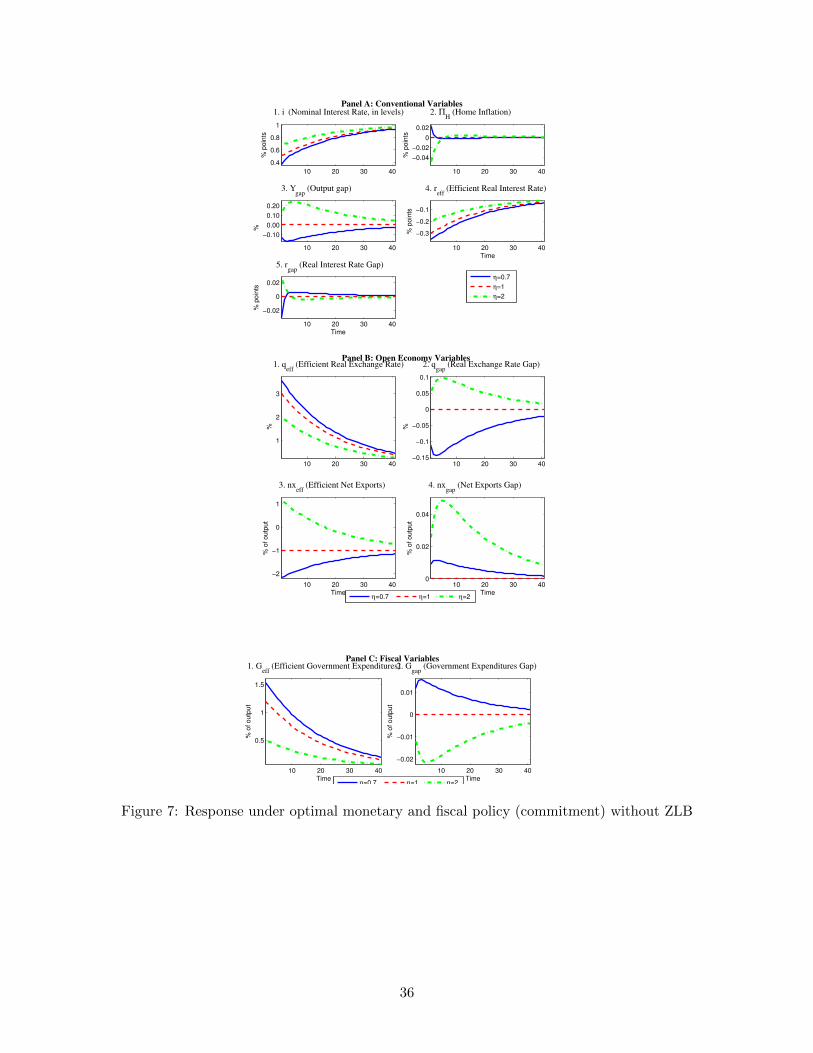
10 20 30 40

0.4

0.6

0.8

1

Panel A: Conventional Variables

1. i (Nominal Interest Rate, in levels)

% p

oin

ts

10 20 30 40

−0.04

−0.02

0

0.02

2. ΠH

(Home Inflation)

% p

oin

ts

10 20 30 40

−0.10

0.00

0.10

0.20

3. Ygap

(Output gap)

%

10 20 30 40

−0.3

−0.2

−0.1

Time

4. reff

(Efficient Real Interest Rate)

% p

oin

ts

10 20 30 40

−0.02

0

0.02

Time

5. rgap

(Real Interest Rate Gap) %

po

ints

η=0.7

η=1

η=2

10 20 30 40

1

2

3

Panel B: Open Economy Variables1. q

eff (Efficient Real Exchange Rate)

%

10 20 30 40−0.15

−0.1

−0.05

0

0.05

0.1

2. qgap

(Real Exchange Rate Gap)

%

10 20 30 40

−2

−1

0

1

Time

3. nxeff

(Efficient Net Exports)

% o

f outp

ut

10 20 30 40 0

0.02

0.04

Time

4. nxgap

(Net Exports Gap)

% o

f outp

ut

η=0.7 η=1 η=2

10 20 30 40

0.5

1

1.5

Panel C: Fiscal Variables

Time

1. Geff

(Efficient Government Expenditures)

% o

f outp

ut

10 20 30 40

−0.02

−0.01

0

0.01

Time

2. Ggap

(Government Expenditures Gap)

% o

f outp

ut

η=0.7 η=1 η=2

Figure 7: Response under optimal monetary and fiscal policy (commitment) without ZLB

36

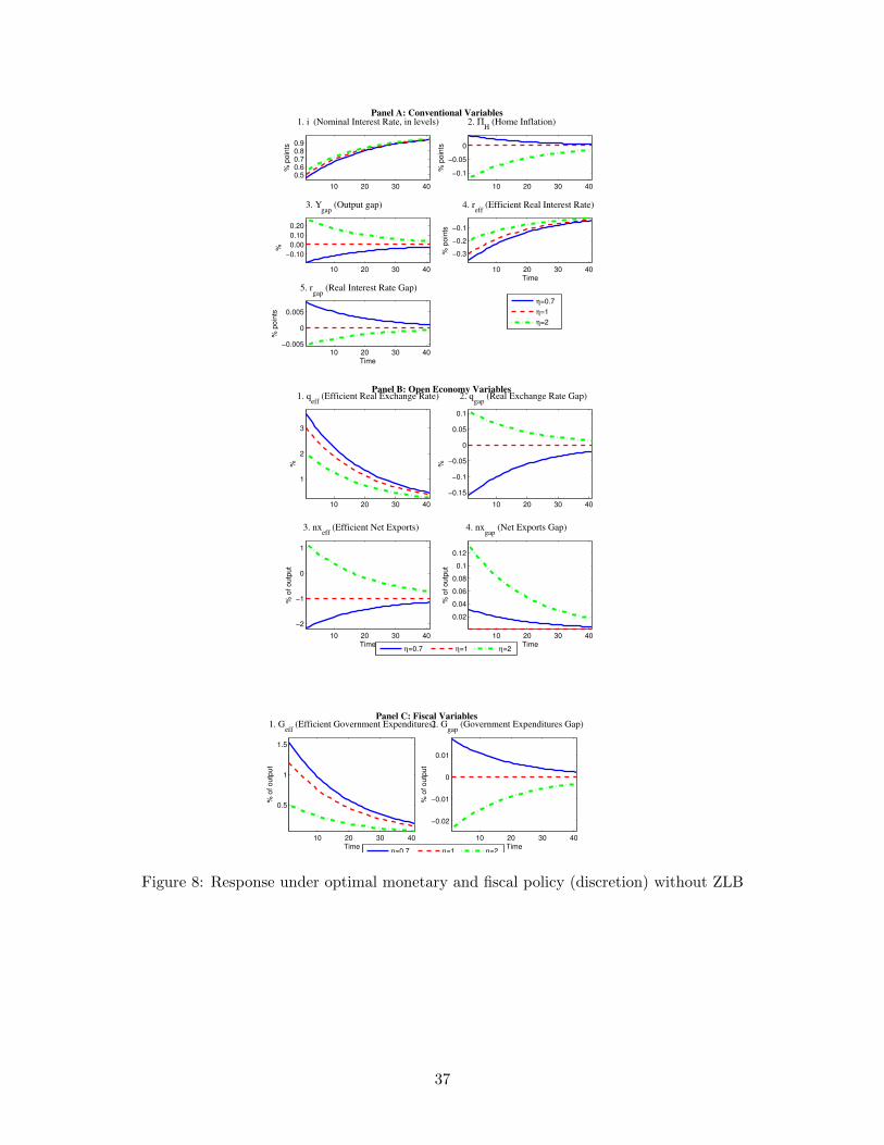
10 20 30 40

0.50.60.70.80.9

Panel A: Conventional Variables

1. i (Nominal Interest Rate, in levels)

% p

oin

ts

10 20 30 40

−0.1

−0.05

0

2. ΠH

(Home Inflation)

% p

oin

ts

10 20 30 40

−0.10

0.00

0.10

0.20

3. Ygap

(Output gap)

%

10 20 30 40

−0.3

−0.2

−0.1

Time

4. reff

(Efficient Real Interest Rate)

% p

oin

ts

10 20 30 40−0.005

0

0.005

Time

5. rgap

(Real Interest Rate Gap)

% p

oin

ts

η=0.7

η=1

η=2

10 20 30 40

1

2

3

Panel B: Open Economy Variables1. q

eff (Efficient Real Exchange Rate)

%

10 20 30 40

−0.15

−0.1

−0.05

0

0.05

0.1

2. qgap

(Real Exchange Rate Gap)

%

10 20 30 40

−2

−1

0

1

Time

3. nxeff

(Efficient Net Exports)

% o

f outp

ut

10 20 30 40

0.02

0.04

0.06

0.08

0.1

0.12

Time

4. nxgap

(Net Exports Gap)

% o

f outp

ut

η=0.7 η=1 η=2

10 20 30 40

0.5

1

1.5

Panel C: Fiscal Variables

Time

1. Geff

(Efficient Government Expenditures)

% o

f outp

ut

10 20 30 40

−0.02

−0.01

0

0.01

Time

2. Ggap

(Government Expenditures Gap)

% o

f outp

ut

η=0.7 η=1 η=2

Figure 8: Response under optimal monetary and fiscal policy (discretion) without ZLB

37

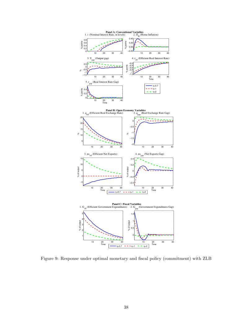
10 20 30 40 0

0.2

0.4

0.6

0.8

Panel A: Conventional Variables

1. i (Nominal Interest Rate, in levels)

% p

oin

ts

10 20 30 40−0.20

0.00

0.20

0.40

2. ΠH

(Home Inflation)

% p

oin

ts

10 20 30 40−1.5

−1

−0.5

0

0.5

3. Ygap

(Output gap)

%

10 20 30 40

−1.2 −1−0.8−0.6−0.4−0.2

Time

4. reff

(Efficient Real Interest Rate)

% p

oin

ts

10 20 30 40

0

0.2

0.4

Time

5. rgap

(Real Interest Rate Gap) %

po

ints

η=0.7

η=1

η=2

10 20 30 40

5

10

15

20

25

Panel B: Open Economy Variables1. q

eff (Efficient Real Exchange Rate)

%

10 20 30 40

−2

−1.5

−1

−0.5

0

2. qgap

(Real Exchange Rate Gap)

%

10 20 30 40

−5

0

5

10

15

Time

3. nxeff

(Efficient Net Exports)

% o

f outp

ut

10 20 30 40

−0.4

−0.2

0

0.2

0.4

Time

4. nxgap

(Net Exports Gap)

% o

f outp

ut

η=0.7 η=1 η=2

10 20 30 40

1

2

3

4

5

Panel C: Fiscal Variables

Time

1. Geff

(Efficient Government Expenditures)

% o

f outp

ut

10 20 30 40

0

0.5

1

1.5

Time

2. Ggap

(Government Expenditures Gap)

% o

f outp

ut

η=0.7 η=1 η=2

Figure 9: Response under optimal monetary and fiscal policy (commitment) with ZLB

38

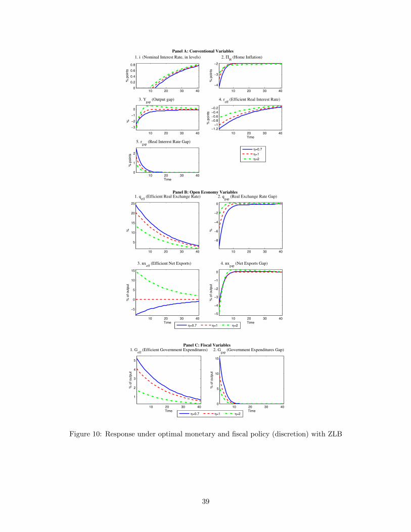
10 20 30 40 0

0.2

0.4

0.6

0.8

Panel A: Conventional Variables

1. i (Nominal Interest Rate, in levels)

% p

oin

ts

10 20 30 40

−4

−3

−2

2. ΠH

(Home Inflation)

% p

oin

ts

10 20 30 40

−3

−2

−1

0

3. Ygap

(Output gap)

%

10 20 30 40

−1.2

−1

−0.8

−0.6

−0.4

−0.2

Time

4. reff

(Efficient Real Interest Rate)

% p

oin

ts

10 20 30 400

1

2

Time

5. rgap

(Real Interest Rate Gap)

% p

oin

ts

η=0.7

η=1

η=2

10 20 30 40

5

10

15

20

25

Panel B: Open Economy Variables1. q

eff (Efficient Real Exchange Rate)

%

10 20 30 40

−8

−6

−4

−2

0

2. qgap

(Real Exchange Rate Gap)

%

10 20 30 40

−5

0

5

10

15

Time

3. nxeff

(Efficient Net Exports)

% o

f outp

ut

10 20 30 40

−5

−4

−3

−2

−1

0

Time

4. nxgap

(Net Exports Gap)

% o

f outp

ut

η=0.7 η=1 η=2

10 20 30 40

1

2

3

4

5

Panel C: Fiscal Variables

Time

1. Geff

(Efficient Government Expenditures)

% o

f outp

ut

10 20 30 40 0

5

10

15

Time

2. Ggap

(Government Expenditures Gap)

% o

f outp

ut

η=0.7 η=1 η=2

Figure 10: Response under optimal monetary and fiscal policy (discretion) with ZLB

39

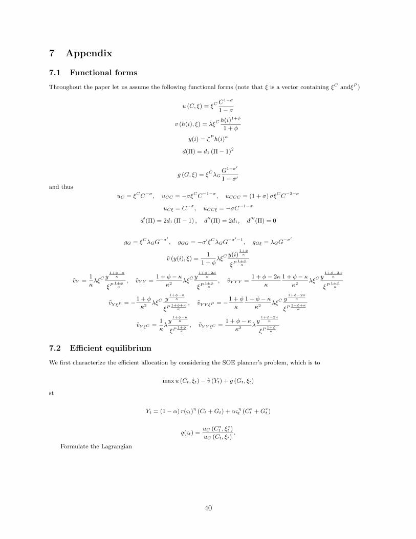
7 Appendix

7.1 Functional forms

Throughout the paper let us assume the following functional forms (note that ξ is a vector containing ξC andξP )

u (C, ξ) = ξCC1−σ

1− σ

v (h(i), ξ) = λξCh(i)1+φ

1 + φ

y(i) = ξPh(i)κ

d(Π) = d1 (Π− 1)2

g (G, ξ) = ξCλGG1−σ′

1− σ′and thus

uC = ξCC−σ, uCC = −σξCC−1−σ, uCCC = (1 + σ)σξCC−2−σ

uCξ = C−σ, uCCξ = −σC−1−σ

d′(Π) = 2d1 (Π− 1) , d′′(Π) = 2d1, d′′′(Π) = 0

gG = ξCλGG−σ′ , gGG = −σ′ξCλGG−σ

′−1, gGξ = λGG−σ′

v (y(i), ξ) =1

1 + φλξC

y(i)1+φκ

ξP1+φκ

vY =1

κλξC

y1+φ−κκ

ξP1+φκ

, vY Y =1 + φ− κ

κ2λξC

y1+φ−2κ

κ

ξP1+φκ

, vY Y Y =1 + φ− 2κ

κ

1 + φ− κκ2

λξCy

1+φ−3κκ

ξP1+φκ

vY ξP = −1 + φ

κ2λξC

y1+φ−κκ

ξP1+φ+κκ

, vY Y ξP = −1 + φ

κ

1 + φ− κκ2

λξCy

1+φ−2κκ

ξP1+φ+κκ

vY ξC =1

κλy

1+φ−κκ

ξP1+φκ

, vY Y ξC =1 + φ− κ

κ2λy

1+φ−2κκ

ξP1+φκ

7.2 Efficient equilibrium

We first characterize the efficient allocation by considering the SOE planner’s problem, which is to

maxu (Ct, ξt)− v (Yt) + g (Gt, ξt)

st

Yt = (1− α) r(ςt)η (Ct +Gt) + αςηt (C∗t +G∗t )

q(ςt) =uC (C∗t , ξ

∗t )

uC (Ct, ξt).

Formulate the Lagrangian

40

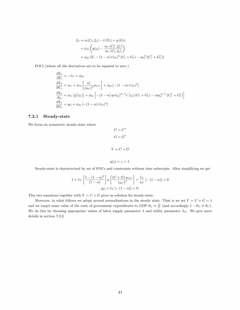
Lt = u (Ct, ξt)− v (Yt) + g (Gt)

+ φ1t

(q(ςt)−

uC (C∗t , ξ∗t )

uC (Ct, ξt)

)+ φ2t (Yt − (1− α) r(ςt)

η (Ct +Gt)− αςηt (C∗t +G∗t ))

FOCs (where all the derivatives are to be equated to zero )

∂Lt∂Yt

= −vY + φ2t

∂Lt∂Ct

= uC + φ1t

[u∗c

(uC)2uCC

]+ φ2t [− (1− α) r(ςt)

η]

∂Lt∂ςt

= φ1t

[q′(ςt)

]+ φ2t

[− (1− α) ηr(ςt)

η−1r′(ςt) (Ct +Gt)− αηςη−1

t (C∗t +G∗t )]

∂Lt∂Gt

= gG + φ2t [− (1− α) r(ςt)η]

7.2.1 Steady-state

We focus on symmetric steady-state where

C = C∗

G = G∗

Y = C +G

q(ς) = ς = 1.

Steady-state is characterized by set of FOCs and constraints without time subscripts. After simplifying we get

1 + vY

[1− (1− α)2

(1− α)

]η

[(C +G)uCC

(uC)2

]+vYuC

[− (1− α)] = 0

gG + vY [− (1− α)] = 0.

This two equations together with Y = C +G gives us solution for steady-state.

Moreover, in what follows we adopt several normalizations in the steady state. That is we set Y = C + G = 1

and we target some value of the ratio of government expenditures to GDP θG ≡ GY

(and accordingly 1 − θG ≡ θC).

We do this by choosing appropriate values of labor supply parameter λ and utility parameter λG. We give more

details in section 7.3.2.

41

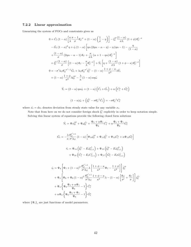
7.2.2 Linear approximation

Linearizing the system of FOCs and constraints gives us

0 = Ct (1− α)

[κ

λ

σ − 1

σθ−σC + (1− α)

(1

σ− η)]− ξPt

(1− α)

σλ(1 + φ) θ1−σC

− Gt (1− α)2 η + ςt (1− α)

[ηα (2ηα− α− η)− η (ηα− 1)− η

(1− α)

+(1− α)

σ(2ηα− α− 1) θC +

κ

σλ(α+ 1− ηα) θ1−σC

]+ ξCt

(1− α)

σ

[(1− α) θC −

κ

λθ1−σC

]+ Yt

[η +

(1− α)

σλ(1 + φ− κ) θ1−σC

]0 = −σ′λGθ−σ

′−1G Gt + λGθ

−σ′G ξCt − (1− α)

1 + φ− κκ2

λYt

+ (1− α)1 + φ

κ2λξPt −

λ

κ(1− α)αηςt

Yt = (2− α) ηαςt + (1− α)(Ct + Gt

)+ α

(C∗t + G∗t

)

(1− α)ςt +(ξCt − σθ

−1C Ct

)= −σθ−1

C C∗t

where xt = dxt denotes deviation from steady state value for any variable xt.

Note that from here on we do not consider foreign shock ξ∗t explicitly in order to keep notation simple.

Solving this linear system of equations provide the following closed form solutions

Yt = Ψ7ξPt + Ψ8ξCt +

Ψ5 + αΨ1

Ψ6C∗t + α

Ψ5 + Ψ1

Ψ6G∗t

Gt = −λκ

θσ′+1G

σ′λG(1− α)

[Ψ10ξ

Pt + Ψ11ξCt + Ψ12C∗t + αΨ13G∗t

]

rt = Ψ14

(ξCt − Et ˆξCt+1

)+ Ψ15

(ξPt − Et ˆξPt+1

)+ Ψ16

(C∗t − Et ˆC∗t+1

)+ Ψ17

(G∗t − Et ˆG∗t+1

)

ςt = Ψ4

[Ψ7 + (1− α)2

θσ′+1G

σ′λGλ

[1 + φ− κ

κ2Ψ7 −

1 + φ

κ2

]]ξPt

+ Ψ4

[Ψ8 + Ψ8 (1− α)2

θσ′+1G

σ′λG

1 + φ− κκ2

λ− (1− α)

[θGσ′

+θCσ

]]ξCt

+ Ψ4

{Ψ9

Ψ5 + αΨ1

Ψ6− 1

}C∗t

+ αΨ4

{Ψ9

Ψ5 + Ψ1

Ψ6− 1

}G∗t

where {Ψi}i are just functions of model parameters.

42

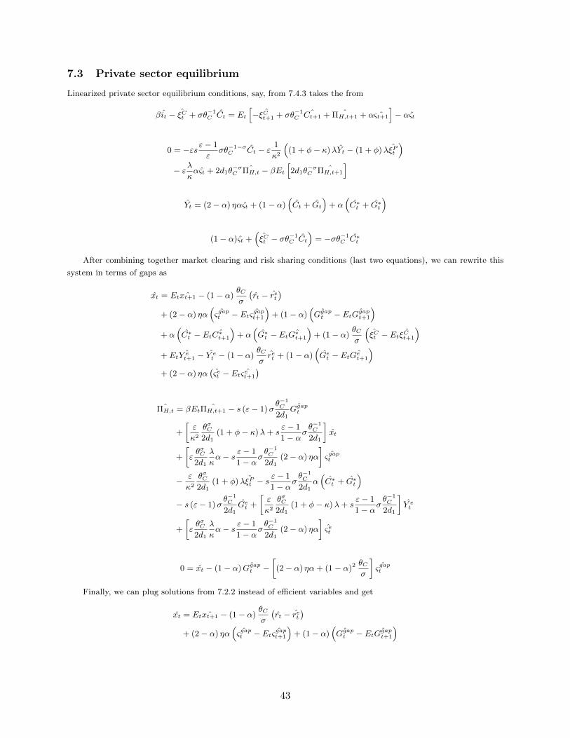
7.3 Private sector equilibrium

Linearized private sector equilibrium conditions, say, from 7.4.3 takes the from

βit − ξCt + σθ−1C Ct = Et

[− ˆξCt+1 + σθ−1

CˆCt+1 + ˆΠH,t+1 + α ˆςt+1

]− αςt

0 = −εsε− 1

εσθ−1−σ

C Ct − ε1

κ2

((1 + φ− κ)λYt − (1 + φ)λξPt

)− ελ

καςt + 2d1θ

−σC

ˆΠH,t − βEt[2d1θ

−σC

ˆΠH,t+1

]

Yt = (2− α) ηαςt + (1− α)(Ct + Gt

)+ α

(C∗t + G∗t

)

(1− α)ςt +(ξCt − σθ

−1C Ct

)= −σθ−1

C C∗t

After combining together market clearing and risk sharing conditions (last two equations), we can rewrite this

system in terms of gaps as

xt = Et ˆxt+1 − (1− α)θCσ

(rt − ret

)+ (2− α) ηα

(ˆςgapt − Et ˆςgapt+1

)+ (1− α)

(ˆGgapt − Et ˆGgapt+1

)+ α

(C∗t − Et ˆC∗t+1

)+ α

(G∗t − Et ˆG∗t+1

)+ (1− α)

θCσ

(ξCt − Et ˆξCt+1

)+ Et ˆY et+1 − Y et − (1− α)

θCσret + (1− α)

(Get − Et ˆGet+1

)+ (2− α) ηα

(ςet − Et ˆςet+1

)

ˆΠH,t = βEt ˆΠH,t+1 − s (ε− 1)σθ−1C

2d1ˆGgapt

+

[ε

κ2

θσC2d1

(1 + φ− κ)λ+ sε− 1

1− ασθ−1C

2d1

]xt

+

[εθσC2d1

λ

κα− s ε− 1

1− ασθ−1C

2d1(2− α) ηα

]ˆςgapt

− ε

κ2

θσC2d1

(1 + φ)λξPt − sε− 1

1− ασθ−1C

2d1α(C∗t + G∗t

)− s (ε− 1)σ

θ−1C

2d1Get +

[ε

κ2

θσC2d1

(1 + φ− κ)λ+ sε− 1

1− ασθ−1C

2d1

]Y et

+

[εθσC2d1

λ

κα− s ε− 1

1− ασθ−1C

2d1(2− α) ηα

]ςet

0 = xt − (1− α) ˆGgapt −[(2− α) ηα+ (1− α)2

θCσ

]ˆςgapt

Finally, we can plug solutions from 7.2.2 instead of efficient variables and get

xt = Et ˆxt+1 − (1− α)θCσ

(rt − ret

)+ (2− α) ηα

(ˆςgapt − Et ˆςgapt+1

)+ (1− α)

(ˆGgapt − Et ˆGgapt+1

)

43

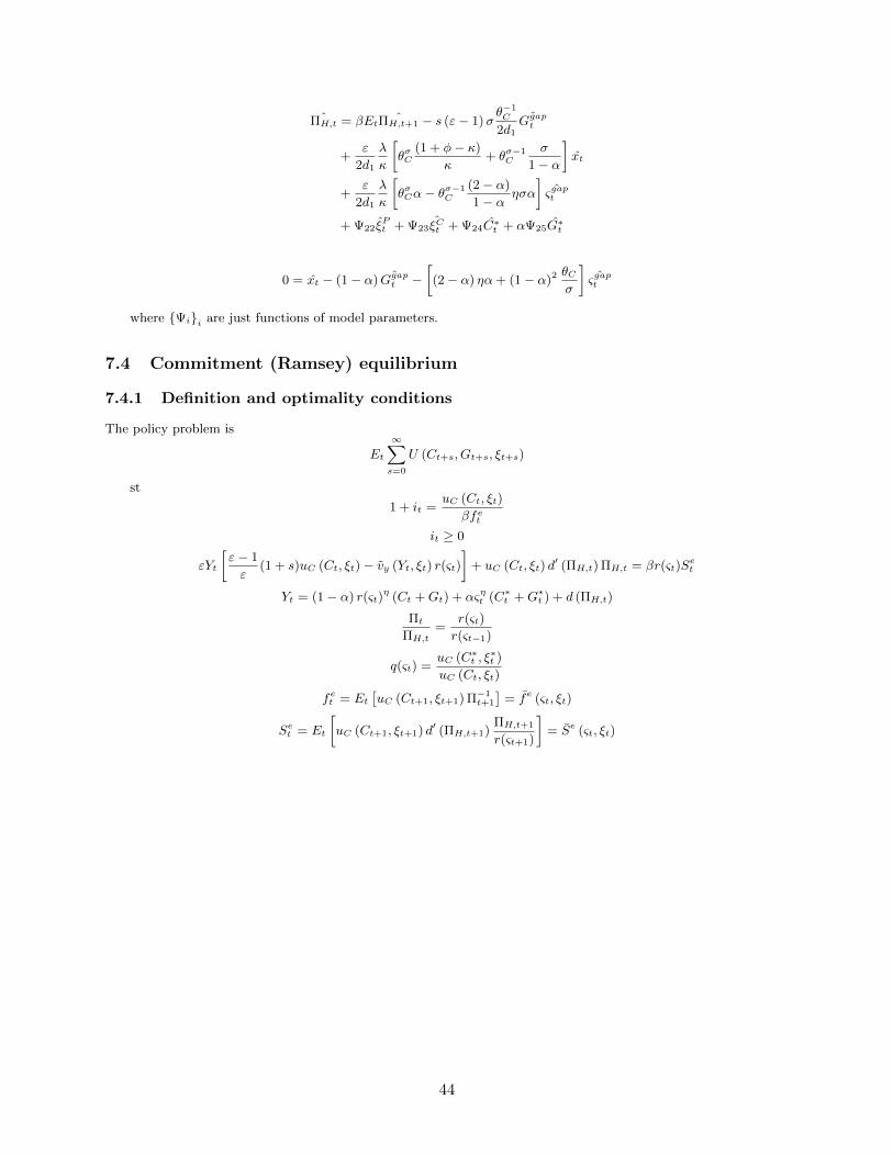
ˆΠH,t = βEt ˆΠH,t+1 − s (ε− 1)σθ−1C

2d1ˆGgapt

+ε

2d1

λ

κ

[θσC

(1 + φ− κ)

κ+ θσ−1

C

σ

1− α

]xt

+ε

2d1

λ

κ

[θσCα− θσ−1

C

(2− α)

1− α ησα

]ˆςgapt

+ Ψ22ξPt + Ψ23ξCt + Ψ24C∗t + αΨ25G∗t

0 = xt − (1− α) ˆGgapt −[(2− α) ηα+ (1− α)2

θCσ

]ˆςgapt

where {Ψi}i are just functions of model parameters.

7.4 Commitment (Ramsey) equilibrium

7.4.1 Definition and optimality conditions

The policy problem is

Et

∞∑s=0

U (Ct+s, Gt+s, ξt+s)

st

1 + it =uC (Ct, ξt)

βfet

it ≥ 0

εYt

[ε− 1

ε(1 + s)uC (Ct, ξt)− vy (Yt, ξt) r(ςt)

]+ uC (Ct, ξt) d

′ (ΠH,t) ΠH,t = βr(ςt)Set

Yt = (1− α) r(ςt)η (Ct +Gt) + αςηt (C∗t +G∗t ) + d (ΠH,t)

Πt

ΠH,t=

r(ςt)

r(ςt−1)

q(ςt) =uC (C∗t , ξ

∗t )

uC (Ct, ξt)

fet = Et[uC (Ct+1, ξt+1) Π−1

t+1

]= fe (ςt, ξt)

Set = Et

[uC (Ct+1, ξt+1) d′ (ΠH,t+1)

ΠH,t+1

r(ςt+1)

]= Se (ςt, ξt)

44

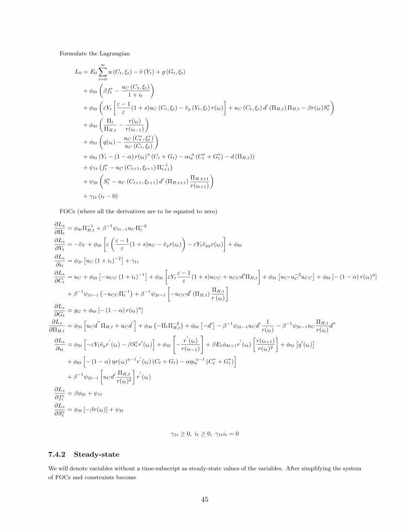
Formulate the Lagrangian

L0 = E0

∞∑t=0

u (Ct, ξt)− v (Yt) + g (Gt, ξt)

+ φ2t

(βfet −

uC (Ct, ξt)

1 + it

)+ φ3t

(εYt

[ε− 1

ε(1 + s)uC (Ct, ξt)− vy (Yt, ξt) r(ςt)

]+ uC (Ct, ξt) d

′ (ΠH,t) ΠH,t − βr(ςt)Set)

+ φ4t

(Πt

ΠH,t− r(ςt)

r(ςt−1)

)+ φ5t

(q(ςt)−

uC (C∗t , ξ∗t )

uC (Ct, ξt)

)+ φ6t (Yt − (1− α) r(ςt)

η (Ct +Gt)− αςηt (C∗t +G∗t )− d (ΠH,t))

+ ψ1t

(fet − uC (Ct+1, ξt+1) Π−1

t+1

)+ ψ2t

(Set − uC (Ct+1, ξt+1) d′ (ΠH,t+1)

ΠH,t+1

r(ςt+1)

)+ γ1t (it − 0)

FOCs (where all the derivatives are to be equated to zero)

∂Ls∂Πt

= φ4tΠ−1H,t + β−1ψ1t−1uCΠ−2

t

∂Ls∂Yt

= −vY + φ3t

[ε

(ε− 1

ε(1 + s)uC − vyr(ςt)

)− εYtvyyr(ςt)

]+ φ6t

∂Ls∂it

= φ2t

[uC (1 + it)

−2]+ γ1t

∂Ls∂Ct

= uC + φ2t

[−uCC (1 + it)

−1]+ φ3t

[εYt

ε− 1

ε(1 + s)uCC + uCCd

′ΠH,t

]+ φ5t

[uC∗u

−2C uCC

]+ φ6t [− (1− α) r(ςt)

η]

+ β−1ψ1t−1

(−uCCΠ−1

t

)+ β−1ψ2t−1

[−uCCd′ (ΠH,t)

ΠH,t

r (ςt)

]∂Ls∂Gt

= gG + φ6t [− (1− α) r(ςt)η]

∂Ls∂ΠH,t

= φ3t

[uCd

′′ΠH,t + uCd

′]+ φ4t

(−ΠtΠ

−2H,t

)+ φ6t

[−d′

]− β−1ψ2t−1uCd

′ 1

r(ςt)− β−1ψ2t−1uC

ΠH,t

r(ςt)d′′

∂Ls∂ςt

= φ3t

[−εYtvyr

′(ςt)− βSet r′(ςt)

]+ φ4t

[− r

′(ςt)

r(ςt−1)

]+ βEtφ4t+1r

′(ςt)

[r(ςt+1)

r(ςt)2

]+ φ5t

[q′(ςt)

]+ φ6t

[− (1− α) ηr(ςt)

η−1r′(ςt) (Ct +Gt)− αηςη−1

t (C∗t +G∗t )]

+ β−1ψ2t−1

[uCd

′ ΠH,t

r(ςt)2

]r′(ςt)

∂Ls∂fet

= βφ2t + ψ1t

∂Ls∂Set

= φ3t [−βr(ςt)] + ψ2t

γ1t ≥ 0, it ≥ 0, γ1tit = 0

7.4.2 Steady-state

We will denote variables without a time-subscript as steady-state values of the variables. After simplifying the system

of FOCs and constraints become

45

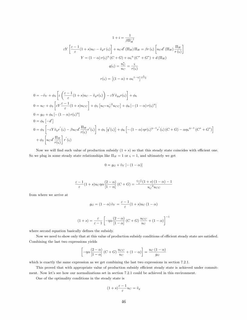
1 + i =1

βΠ−1H

εY

[ε− 1

ε(1 + s)uC − vyr (ς)

]+ uCd

′ (ΠH) ΠH = βr (ς)

[uCd

′ (ΠH)ΠH

r (ς)

]Y = (1− α) r(ς)η (C +G) + αςη (C∗ +G∗) + d (ΠH)

q(ς) =u∗CuC

=ς

r(ς)

r(ς) =[(1− α) + ας1−η

] 11−η

0 = −vY + φ3

[ε

(ε− 1

ε(1 + s)uC − vyr(ς)

)− εY vyyr(ς)

]+ φ6

0 = uC + φ3

[εY

ε− 1

ε(1 + s)uCC

]+ φ5

[uC∗u

−2C uCC

]+ φ6 [− (1− α) r(ς)η]

0 = gG + φ6 [− (1− α) r(ς)η]

0 = φ6

[−d′

]0 = φ3

[−εY vyr

′(ς)− βuCd′

ΠH

r(ς)r′(ς)

]+ φ5

[q′(ς)

]+ φ6

[− (1− α) ηr(ς)η−1r

′(ς) (C +G)− αηςη−1 (C∗ +G∗)

]+ φ3

[uCd

′ ΠH

r(ς)

]r′(ς)

Now we will find such value of production subsidy (1 + s) so that this steady state coincides with efficient one.

So we plug in some steady state relationships like ΠH = 1 or ς = 1, and ultimately we get

0 = gG + vY [− (1− α)]

ε− 1

ε(1 + s)uCηα

(2− α)

[1− α](C +G) =

ε−1ε

(1 + s) (1− α)− 1

u−2C uCC

from where we arrive at

gG = (1− α) vY =ε− 1

ε(1 + s)uC (1− α)

(1 + s) =ε

ε− 1

[−ηα (2− α)

[1− α](C +G)

uCCuC

+ (1− α)

]−1

where second equation basically defines the subsidy.

Now we need to show only that at this value of production subsidy conditions of efficient steady state are satisfied.

Combining the last two expressions yields[−ηα (2− α)

[1− α](C +G)

uCCuC

+ (1− α)

]=uC (1− α)

gG

which is exactly the same expression as we get combining the last two expressions in section 7.2.1.

This proved that with appropriate value of production subsidy efficient steady state is achieved under commit-

ment. Now let’s see how our normalizations set in section 7.2.1 could be achieved in this environment.

One of the optimality conditions in the steady state is

(1 + s)ε− 1

εuC = vy

46

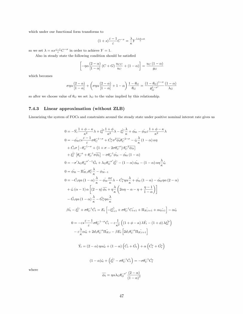
which under our functional form transforms to

(1 + s)ε− 1

εC−σ =

λ

κY

1+φ−κκ

so we set λ = κs ε−1εC−σ in order to achieve Y = 1.

Also in steady state the following condition should be satisfied[−ηα (2− α)

[1− α](C +G)

uCCuC

+ (1− α)

]=uC (1− α)

gG

which becomes

σηα(2− α)

[1− α]+

(σηα

(2− α)

[1− α]+ 1− α

)1− θGθG

=(1− θG)1−σ

θ1−σ′

G

(1− α)

λG

so after we choose value of θG we set λG to the value implied by this relationship.

7.4.3 Linear approximation (without ZLB)

Linearizing the system of FOCs and constraints around the steady state under positive nominal interest rate gives us

0 = −Yt1 + φ− κ

κ2λ+ ξPt

1 + φ

κ2λ− ξCt

λ

κ+ φ6t − φ3tε

1 + φ− κκ2

λ

0 = −φ3tεsε− 1

εσθ−1−σ

C + C∗t σ2φ5θ

−2−σC − ςt

λ

κ(1− α)αη

+ Ctσ[−θ−1−σ

C +(1 + σ − 2σθ−σC

)θ−2C φ5t

]+ ξCt

[θ−σC + θ−1

C σφ5

]− σθ−1

C φ5t − φ6t (1− α)

0 = −σ′λGθ−σ′−1

G Gt + λGθ−σ′G ξCt − (1− α) φ6t − (1− α)αη

λ

κςt

0 = φ3t − ˆΠH,tθσCλ

κ− ˆφ3t−1

0 = −Ctηα (1− α)λ

κ− φ3t

αε

κλ− C∗t ηα

λ

κ+ φ5t (1− α)− φ6tηα (2− α)

+ ςt (α− 1)α

[(2− η)φ5 + η

λ

κ

(2αη − α− η +

η − 1

1− α

)]− Gtηα (1− α)

λ

κ− G∗t ηα

λ

κ

βit − ξCt + σθ−1C Ct = Et

[− ˆξCt+1 + σθ−1

CˆCt+1 + ˆΠH,t+1 + α ˆςt+1

]− αςt

0 = −εsε− 1

εσθ−1−σ

C Ct − ε1

κ2

((1 + φ− κ)λYt − (1 + φ)λξPt

)− ελ

καςt + 2d1θ

−σC

ˆΠH,t − βEt[2d1θ

−σC

ˆΠH,t+1

]

Yt = (2− α) ηαςt + (1− α)(Ct + Gt

)+ α

(C∗t + G∗t

)

(1− α)ςt +(ξCt − σθ

−1C Ct

)= −σθ−1

C C∗t

where

φ5 = ηαλGθ−σ′G

(2− α)

(1− α)2

47

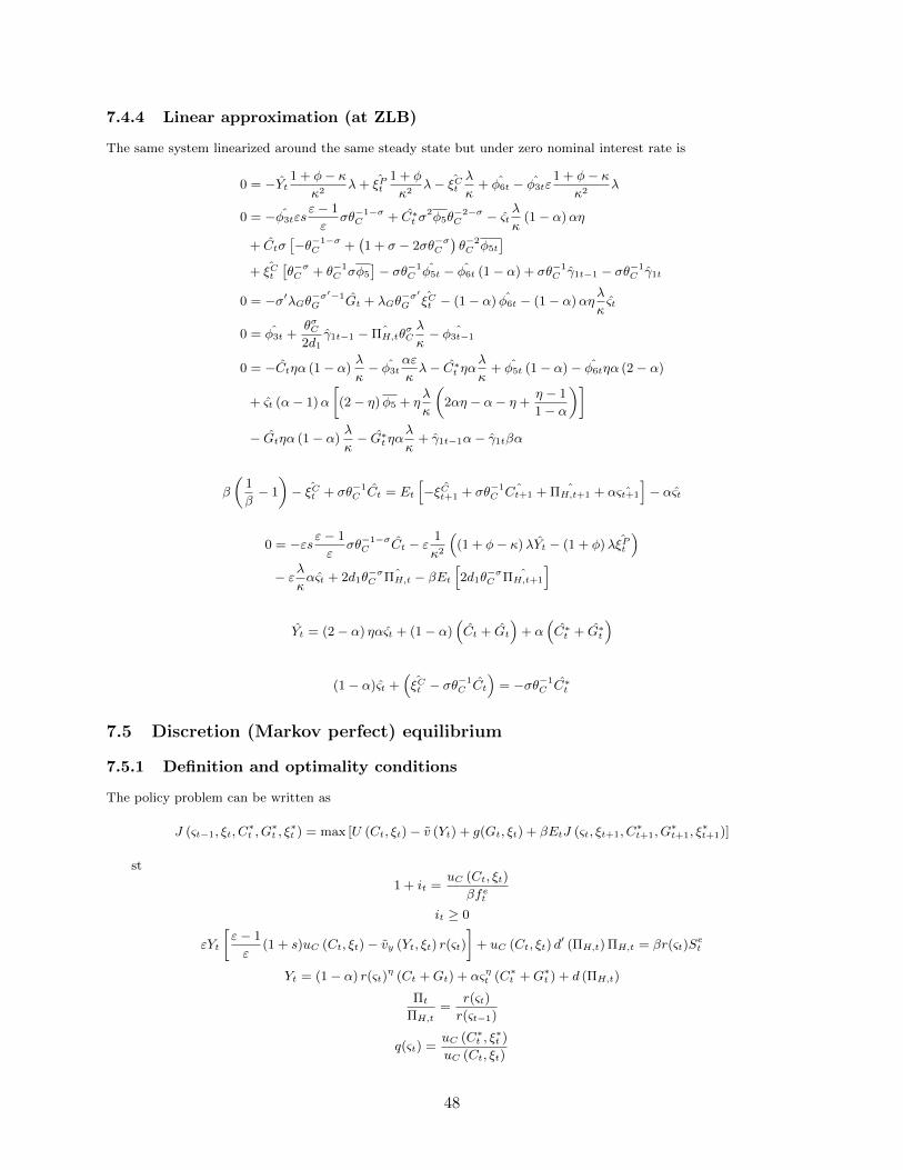
7.4.4 Linear approximation (at ZLB)

The same system linearized around the same steady state but under zero nominal interest rate is

0 = −Yt1 + φ− κ

κ2λ+ ξPt

1 + φ

κ2λ− ξCt

λ

κ+ φ6t − φ3tε

1 + φ− κκ2

λ

0 = −φ3tεsε− 1

εσθ−1−σ

C + C∗t σ2φ5θ

−2−σC − ςt

λ

κ(1− α)αη

+ Ctσ[−θ−1−σ

C +(1 + σ − 2σθ−σC

)θ−2C φ5t

]+ ξCt

[θ−σC + θ−1

C σφ5

]− σθ−1

C φ5t − φ6t (1− α) + σθ−1C γ1t−1 − σθ−1

C γ1t

0 = −σ′λGθ−σ′−1

G Gt + λGθ−σ′G ξCt − (1− α) φ6t − (1− α)αη

λ

κςt

0 = φ3t +θσC2d1

γ1t−1 − ˆΠH,tθσCλ

κ− ˆφ3t−1

0 = −Ctηα (1− α)λ

κ− φ3t

αε

κλ− C∗t ηα

λ

κ+ φ5t (1− α)− φ6tηα (2− α)

+ ςt (α− 1)α

[(2− η)φ5 + η

λ

κ

(2αη − α− η +

η − 1

1− α

)]− Gtηα (1− α)

λ

κ− G∗t ηα

λ

κ+ γ1t−1α− γ1tβα

β

(1

β− 1

)− ξCt + σθ−1

C Ct = Et[− ˆξCt+1 + σθ−1

CˆCt+1 + ˆΠH,t+1 + α ˆςt+1

]− αςt

0 = −εsε− 1

εσθ−1−σ

C Ct − ε1

κ2

((1 + φ− κ)λYt − (1 + φ)λξPt

)− ελ

καςt + 2d1θ

−σC

ˆΠH,t − βEt[2d1θ

−σC

ˆΠH,t+1

]

Yt = (2− α) ηαςt + (1− α)(Ct + Gt

)+ α

(C∗t + G∗t

)

(1− α)ςt +(ξCt − σθ

−1C Ct

)= −σθ−1

C C∗t

7.5 Discretion (Markov perfect) equilibrium

7.5.1 Definition and optimality conditions

The policy problem can be written as

J (ςt−1, ξt, C∗t , G

∗t , ξ∗t ) = max [U (Ct, ξt)− v (Yt) + g(Gt, ξt) + βEtJ (ςt, ξt+1, C

∗t+1, G

∗t+1, ξ

∗t+1)]

st

1 + it =uC (Ct, ξt)

βfet

it ≥ 0

εYt

[ε− 1

ε(1 + s)uC (Ct, ξt)− vy (Yt, ξt) r(ςt)

]+ uC (Ct, ξt) d

′ (ΠH,t) ΠH,t = βr(ςt)Set

Yt = (1− α) r(ςt)η (Ct +Gt) + αςηt (C∗t +G∗t ) + d (ΠH,t)

Πt

ΠH,t=

r(ςt)

r(ςt−1)

q(ςt) =uC (C∗t , ξ

∗t )

uC (Ct, ξt)

48

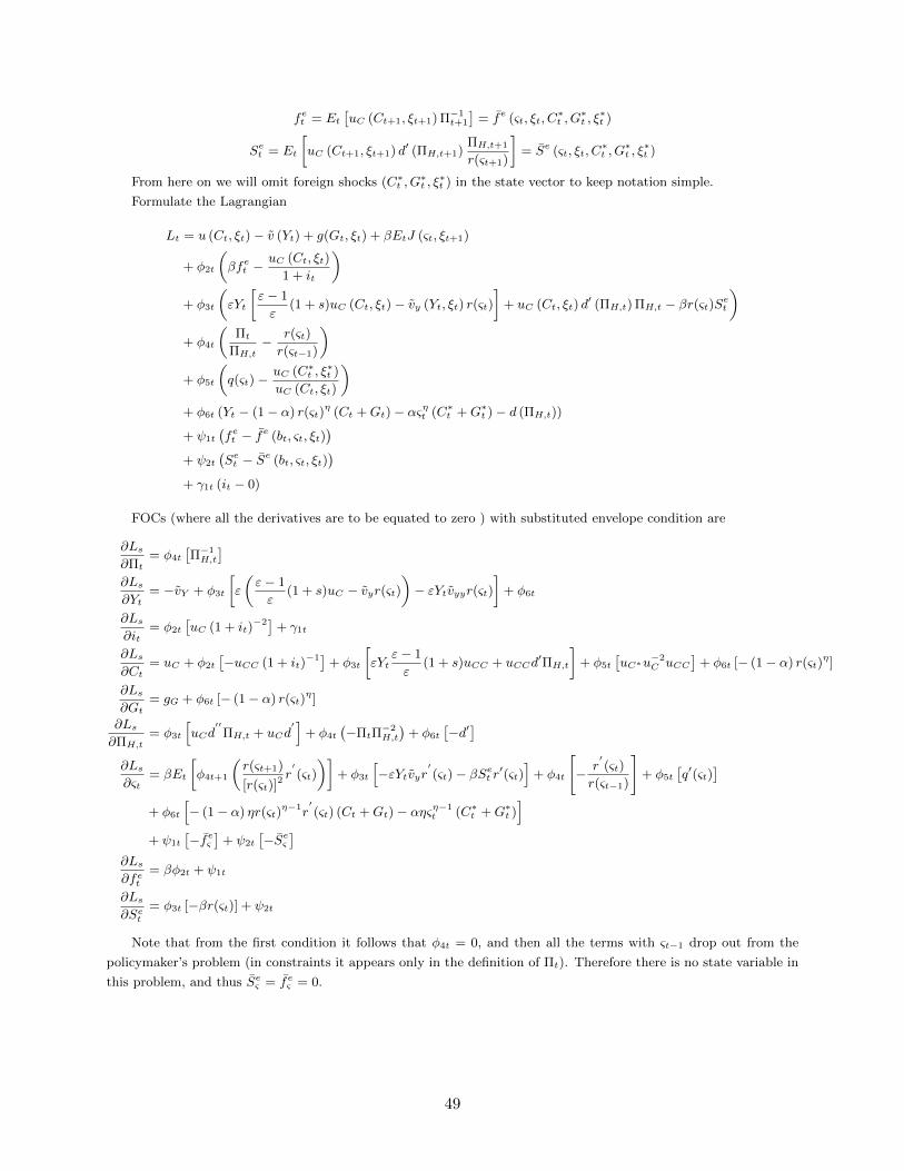
fet = Et[uC (Ct+1, ξt+1) Π−1

t+1

]= fe (ςt, ξt, C

∗t , G

∗t , ξ∗t )

Set = Et

[uC (Ct+1, ξt+1) d′ (ΠH,t+1)

ΠH,t+1

r(ςt+1)

]= Se (ςt, ξt, C

∗t , G

∗t , ξ∗t )

From here on we will omit foreign shocks (C∗t , G∗t , ξ∗t ) in the state vector to keep notation simple.

Formulate the Lagrangian

Lt = u (Ct, ξt)− v (Yt) + g(Gt, ξt) + βEtJ (ςt, ξt+1)

+ φ2t

(βfet −

uC (Ct, ξt)

1 + it

)+ φ3t

(εYt

[ε− 1

ε(1 + s)uC (Ct, ξt)− vy (Yt, ξt) r(ςt)

]+ uC (Ct, ξt) d

′ (ΠH,t) ΠH,t − βr(ςt)Set)

+ φ4t

(Πt

ΠH,t− r(ςt)

r(ςt−1)

)+ φ5t

(q(ςt)−

uC (C∗t , ξ∗t )

uC (Ct, ξt)

)+ φ6t (Yt − (1− α) r(ςt)

η (Ct +Gt)− αςηt (C∗t +G∗t )− d (ΠH,t))

+ ψ1t

(fet − fe (bt, ςt, ξt)

)+ ψ2t

(Set − Se (bt, ςt, ξt)

)+ γ1t (it − 0)

FOCs (where all the derivatives are to be equated to zero ) with substituted envelope condition are

∂Ls∂Πt

= φ4t

[Π−1H,t

]∂Ls∂Yt

= −vY + φ3t

[ε

(ε− 1

ε(1 + s)uC − vyr(ςt)

)− εYtvyyr(ςt)

]+ φ6t

∂Ls∂it

= φ2t

[uC (1 + it)

−2]+ γ1t

∂Ls∂Ct

= uC + φ2t

[−uCC (1 + it)

−1]+ φ3t

[εYt

ε− 1

ε(1 + s)uCC + uCCd

′ΠH,t

]+ φ5t

[uC∗u

−2C uCC

]+ φ6t [− (1− α) r(ςt)

η]

∂Ls∂Gt

= gG + φ6t [− (1− α) r(ςt)η]

∂Ls∂ΠH,t

= φ3t

[uCd

′′ΠH,t + uCd

′]+ φ4t

(−ΠtΠ

−2H,t

)+ φ6t

[−d′

]∂Ls∂ςt

= βEt

[φ4t+1

(r(ςt+1)

[r(ςt)]2 r′(ςt)

)]+ φ3t

[−εYtvyr

′(ςt)− βSet r′(ςt)

]+ φ4t

[− r

′(ςt)

r(ςt−1)

]+ φ5t

[q′(ςt)

]+ φ6t

[− (1− α) ηr(ςt)

η−1r′(ςt) (Ct +Gt)− αηςη−1

t (C∗t +G∗t )]

+ ψ1t

[−feς

]+ ψ2t

[−Seς

]∂Ls∂fet

= βφ2t + ψ1t

∂Ls∂Set

= φ3t [−βr(ςt)] + ψ2t

Note that from the first condition it follows that φ4t = 0, and then all the terms with ςt−1 drop out from the

policymaker’s problem (in constraints it appears only in the definition of Πt). Therefore there is no state variable in

this problem, and thus Seς = feς = 0.

49

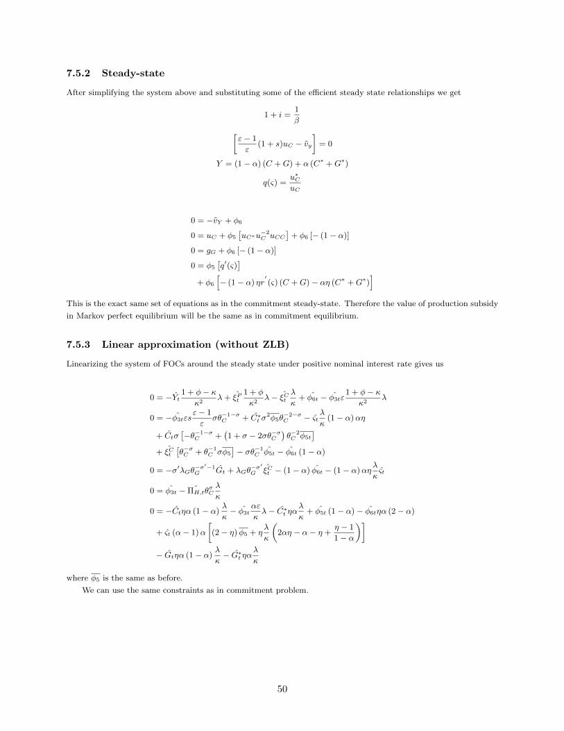
7.5.2 Steady-state

After simplifying the system above and substituting some of the efficient steady state relationships we get

1 + i =1

β[ε− 1

ε(1 + s)uC − vy

]= 0

Y = (1− α) (C +G) + α (C∗ +G∗)

q(ς) =u∗CuC

0 = −vY + φ6

0 = uC + φ5

[uC∗u

−2C uCC

]+ φ6 [− (1− α)]

0 = gG + φ6 [− (1− α)]

0 = φ5

[q′(ς)

]+ φ6

[− (1− α) ηr

′(ς) (C +G)− αη (C∗ +G∗)

]This is the exact same set of equations as in the commitment steady-state. Therefore the value of production subsidy

in Markov perfect equilibrium will be the same as in commitment equilibrium.

7.5.3 Linear approximation (without ZLB)

Linearizing the system of FOCs around the steady state under positive nominal interest rate gives us

0 = −Yt1 + φ− κ

κ2λ+ ξPt

1 + φ

κ2λ− ξCt

λ

κ+ φ6t − φ3tε

1 + φ− κκ2

λ

0 = −φ3tεsε− 1

εσθ−1−σ

C + C∗t σ2φ5θ

−2−σC − ςt

λ

κ(1− α)αη

+ Ctσ[−θ−1−σ

C +(1 + σ − 2σθ−σC

)θ−2C φ5t

]+ ξCt

[θ−σC + θ−1

C σφ5

]− σθ−1

C φ5t − φ6t (1− α)

0 = −σ′λGθ−σ′−1

G Gt + λGθ−σ′G ξCt − (1− α) φ6t − (1− α)αη

λ

κςt

0 = φ3t − ˆΠH,tθσCλ

κ

0 = −Ctηα (1− α)λ

κ− φ3t

αε

κλ− C∗t ηα

λ

κ+ φ5t (1− α)− φ6tηα (2− α)

+ ςt (α− 1)α

[(2− η)φ5 + η

λ

κ

(2αη − α− η +

η − 1

1− α

)]− Gtηα (1− α)

λ

κ− G∗t ηα

λ

κ

where φ5 is the same as before.

We can use the same constraints as in commitment problem.

50

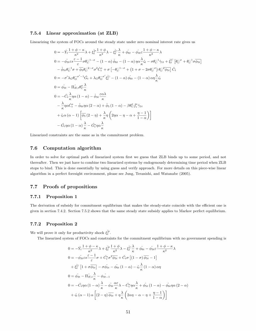
7.5.4 Linear approximation (at ZLB)

Linearizing the system of FOCs around the steady state under zero nominal interest rate gives us

0 = −Yt1 + φ− κ

κ2λ+ ξPt

1 + φ

κ2λ− ξCt

λ

κ+ φ6t − φ3tε

1 + φ− κκ2

λ

0 = −φ3tεsε− 1

εσθ−1−σ

C − (1− α) φ6t − (1− α) ηαλ

κςt − σθ−1

C γ1t + ξCt[θ−σC + θ−1

C σφ5t

]− φ5tθ

−1C σ + φ5θ

−2−σC σ2C∗t + σ

[−θ−1−σ

C +(1 + σ − 2σθ−σC

)θ−2C φ5t

]Ct

0 = −σ′λGθ−σ′−1

G Gt + λGθ−σ′G ξCt − (1− α) φ6t − (1− α)αη

λ

κςt

0 = φ3t − ˆΠH,tθσCλ

κ

0 = −Ctλ

κηα (1− α)− φ3t

εαλ

κ

− λ

κηαC∗t − φ6tηα (2− α) + φ5 (1− α)− βθσC feς γ1t

+ ςtα (α− 1)

[φ5 (2− η) +

λ

κη

(2ηα− η − α+

η − 1

1− α

)]− Gtηα (1− α)

λ

κ− G∗t ηα

λ

κ

Linearized constraints are the same as in the commitment problem.

7.6 Computation algorithm

In order to solve for optimal path of linearized system first we guess that ZLB binds up to some period, and not

thereafter. Then we just have to combine two linearized systems by endogenously determining time period when ZLB

stops to bind. This is done essentially by using guess and verify approach. For more details on this piece-wise linear

algorithm in a perfect foresight environment, please see Jung, Teranishi, and Watanabe (2005).

7.7 Proofs of propositions

7.7.1 Proposition 1

The derivation of subsidy for commitment equilibrium that makes the steady-state coincide with the efficient one is

given in section 7.4.2. Section 7.5.2 shows that the same steady state subsidy applies to Markov perfect equilibrium.

7.7.2 Proposition 2

We will prove it only for productivity shock ξPt .

The linearized system of FOCs and constraints for the commitment equilibrium with no government spending is

0 = −Yt1 + φ− κ

κ2λ+ ξPt

1 + φ

κ2λ− ξCt

λ

κ+ φ6t − φ3tε

1 + φ− κκ2

λ

0 = −φ3tεsε− 1

εσ + C∗t σ

2φ5t + Ctσ[(1− σ)φ5t − 1

]+ ξCt

[1 + σφ5t

]− σφ5t − φ6t (1− α)− ςt

λ

κ(1− α)αη

0 = φ3t − ˆΠH,tλ

κ− ˆφ3t−1

0 = −Ctηα (1− α)λ

κ− φ3t

αε

κλ− C∗t ηα

λ

κ+ φ5t (1− α)− φ6tηα (2− α)

+ ςt (α− 1)α

[(2− η)φ5t + η

λ

κ

(2αη − α− η +

η − 1

1− α

)]

51

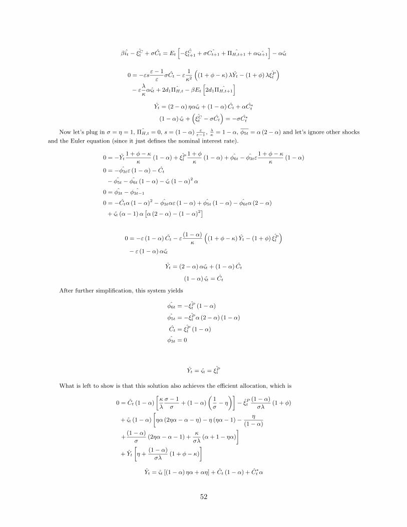
βit − ξCt + σCt = Et[− ˆξCt+1 + σ ˆCt+1 + ˆΠH,t+1 + α ˆςt+1

]− αςt

0 = −εsε− 1

εσCt − ε

1

κ2

((1 + φ− κ)λYt − (1 + φ)λξPt

)− ελ

καςt + 2d1 ˆΠH,t − βEt

[2d1 ˆΠH,t+1

]Yt = (2− α) ηαςt + (1− α) Ct + αC∗t

(1− α) ςt +(ξCt − σCt

)= −σC∗t

Now let’s plug in σ = η = 1, ˆΠH,t = 0, s = (1− α) εε−1

, λκ

= 1− α, φ5t = α (2− α) and let’s ignore other shocks

and the Euler equation (since it just defines the nominal interest rate).

0 = −Yt1 + φ− κ

κ(1− α) + ξPt

1 + φ

κ(1− α) + φ6t − φ3tε

1 + φ− κκ

(1− α)

0 = −φ3tε (1− α)− Ct− φ5t − φ6t (1− α)− ςt (1− α)2 α

0 = φ3t − ˆφ3t−1

0 = −Ctα (1− α)2 − φ3tαε (1− α) + φ5t (1− α)− φ6tα (2− α)

+ ςt (α− 1)α[α (2− α)− (1− α)2

]

0 = −ε (1− α) Ct − ε(1− α)

κ

((1 + φ− κ) Yt − (1 + φ) ξPt

)− ε (1− α)αςt

Yt = (2− α)αςt + (1− α) Ct

(1− α) ςt = Ct

After further simplification, this system yields

φ6t = −ξPt (1− α)

φ5t = −ξPt α (2− α) (1− α)

Ct = ξPt (1− α)

φ3t = 0

Yt = ςt = ξPt

What is left to show is that this solution also achieves the efficient allocation, which is

0 = Ct (1− α)

[κ

λ

σ − 1

σ+ (1− α)

(1

σ− η)]− ξPt

(1− α)

σλ(1 + φ)

+ ςt (1− α)

[ηα (2ηα− α− η)− η (ηα− 1)− η

(1− α)

+(1− α)

σ(2ηα− α− 1) +

κ

σλ(α+ 1− ηα)

]+ Yt

[η +

(1− α)

σλ(1 + φ− κ)

]Yt = ςt [(1− α) ηα+ αη] + Ct (1− α) + C∗t α

52

ςt (1− α) +(−σCt + ξCt

)= −σC∗t

After plugging in values for the special case considered it becomes

0 = −ξPt(1 + φ)

κ+ Yt

[1 +

1 + φ− κκ

]Yt = (2− α)αςt + (1− α) Ct

(1− α) ςt = Ct

which shows clearly that this is the same solution as the commitment one.

7.7.3 Proposition 3

Again, we will prove it only for productivity shock ξPt .

The linearized system of FOCs and constraints for the Markov perfect equilibrium with no government spending

is

0 = −1 + φ− κκ2

λYt +1 + φ

κ2λξPt −

λ

κξCt + φ6t + φ3t

[−ε1 + φ− κ

κ2λ

]0 = −φ3tε

λ

κσ − (1− α) φ6t − (1− α) ηα

λ

κςt

− φ5tσ + φ5tσ2C∗t + σ

[φ5t (1− σ)− 1

]Ct + ξCt

[σφ5t + 1

]0 = φ3t −

λ

κΠH,t

0 = −Ctλ

κηα (1− α)− φ3t

εαλ

κ

− λ

κηαC∗t − φ6tηα (2− α) + φ5t (1− α)

+ ςtα (α− 1)

[φ5t (2− η) +

λ

κη

(2ηα− η − α+

η − 1

1− α

)]

βit − ξCt + σCt = Et[− ˆξCt+1 + σ ˆCt+1 + ˆΠH,t+1 + α ˆςt+1

]− αςt

0 = −εsε− 1

εσCt − ε

1

κ2

((1 + φ− κ)λYt − (1 + φ)λξPt

)− ελ

καςt + 2d1 ˆΠH,t − βEt

[2d1 ˆΠH,t+1

]Yt = (2− α) ηαςt + (1− α) Ct + αC∗t

(1− α) ςt +(ξCt − σCt

)= −σC∗t

The only difference from the commitment problem in 7.7.2 is the absence of the term with ˆφ3t−1 in the third

FOC. Since in the solution to the commitment problem φ3t = 0, it is clear that the same solution as before will satisfy

this system.

7.7.4 Proposition 4

We will prove it only for productivity shock ξPt .

Let’s substitute terms of trade instead of consumption using risk sharing condition and by doing this get rid of

53

consumption in the system of FOCs from 7.4.4 and get

0 = −Yt1 + φ− κ

κ2λ+ ξPt

1 + φ

κ2λ+ φ6t − φ3tε

1 + φ− κκ2

λ

0 = −φ3tεsε− 1

εσ + ςt

[(1− σ)

λ

κηα

(2− α)

[1− α]− 1− λ

καη

](1− α)

− σφ5t − φ6t (1− α) + σγ1t−1 − σγ1t

0 = φ3t +1

2d1γ1t−1 − ˆΠH,t

λ

κ− ˆφ3t−1

0 = −φ3tαε

κλ+ φ5t (1− α)− φ6tηα (2− α)

+ ςt (α− 1)α

[(2− η)

λ

κηα

(2− α)

[1− α]+ η

λ

κ

(2αη − α− η +

η − 1

1− α

)+ η

λ

κ

(1− α)

σ

]+ γ1t−1α− γ1tβα

Next let’s combine some of this conditions to get rid of φ5t and φ6t, and let’s denote

xt ≡ Yt1 + φ− κ

κ2λ

[ηα (2− α) +

(1− α)2

σ

]− ξPt

1 + φ

κ2λ

[ηα (2− α) +

(1− α)2

σ

]− ςt (α− 1)

[(2− η)

λ

κηα2 (2− α)

[1− α]+ ηα

λ

κ

(2 + 2αη − 2α− η +

η − 1

1− α

)− ηα2

σ

λ

κ− (α− 1)

σ

]= xt

1 + φ− κκ2

λ

[ηα (2− α) +

(1− α)2

σ

]− ˆςgapt (α− 1)

[(2− η)

λ

κηα2 (2− α)

[1− α]+ ηα

λ

κ

(2 + 2αη − 2α− η +

η − 1

1− α

)− ηα2

σ

λ

κ− (α− 1)

σ

]+ ξPt

[1 + φ− κ

κ2λ

[ηα (2− α) +

(1− α)2

σ

]Ψ7 −

1 + φ

κ2λ

(ηα (2− α) +

(1− α)2

σ

)− (α− 1)

[(2− η)

λ

κηα2 (2− α)

[1− α]+ ηα

λ

κ

(2 + 2αη − 2α− η +

η − 1

1− α

)− ηα2

σ

λ

κ− (α− 1)

σ

]×

×[(2− α) ηα+

(1− α)2

σ

]−1

Ψ7

]

to get

0 = ˆΠH,t −κ

λφ3t +

κ

λˆφ3t−1 −

1

2d1

κ

λγ1t−1

0 =1

(1 + βα− α)xt + γ1t −

1

(1 + βα− α)γ1t−1

+ φ3tελ

κ

1

(1 + βα− α)

[1 + φ− κ

κ

(ηα (2− α) +

(1− α)2

σ

)+ 1

]

54

After introducing the following notation

λ ≡ 1

(1 + βα− α)

φ1t ≡ γ1tβ ≡ (1 + βα− α)

φ2t ≡ −κ

λφ3t

κ ≡ ελ2

κ2

1

(1 + βα− α)

[1 + φ− κ

κ

(ηα (2− α) +

(1− α)2

σ

)+ 1

]πt ≡ ˆΠH,t

σ ≡ 1

2d1

κ

λ(1 + βα− α)

the same system becomes

λxt + φ1t −1

β˜φ1t−1 − κφ2t = 0

πt + φ2t − ˜φ2t−1 −σ

β˜φ1t−1 = 0

which is isomorphic to Eggertsson and Woodford (2003). Therefore price level target rule will have the same form.

7.7.5 Reformulation of targeting rule and PSE conditions

Note that the same targeting rule as in previous section could be expressed thorugh different gaps, that is

xt = Ytgap 1 + φ− κ

κ2λ

[ηα (2− α) +

(1− α)2

σ

]− ςtgap (α− 1)

[(2− η)

λ

κηα2 (2− α)

[1− α]+ ηα

λ

κ

(2 + 2αη − 2α− η +

η − 1

1− α

)− ηα2

σ

λ

κ− (α− 1)

σ

]where

Ytgap ≡ Yt − ξPt

1 + φ

1 + φ− κ

ςtgap ≡ ςt − ξPt 0.

Then linearized PSE conditions in terms of these gaps could be represented as

Ytgap

= Et ˜Yt+1gap − (1− α)

σrtgap

+ (2− α) ηα (ςtgap − Et ˜ςt+1

gap)

− 1 + φ

1 + φ− κ

(ξPt − Et ˆξPt+1

)

ˆΠH,t = βEt ˆΠH,t+1

+ε

2d1

λ

κ

[(1 + φ− κ)

κ+

σ

1− α

]Ytgap

+ε

2d1

λ

κ

[α− (2− α)

1− α ησα

]ςtgap

+

[ε

2d1

λ

κ

[(1 + φ− κ)

κ+

σ

1− α

](1 + φ

1 + φ− κ −Ψ7

)− ε

2d1

λ

κ

[α− (2− α)

1− α ησα

]Ψ7 + Ψ22

]ξPt

55

Ytgap

=

[(2− α) ηα+

(1− α)2

σ

]ςtgap −

([(2− α) ηα+

(1− α)2

σ− 1

]Ψ7 +

1 + φ

1 + φ− κ

)ξPt

where

rtgap = rt.

7.7.6 Proposition 5

We will prove it only for productivity shock ξPt .

Repeating the steps from the previous subsection, but for the system from 7.5.4 yields

xt = − ˆΠH,tελ2

κ2

[1 + φ− κ

κ

(ηα (2− α) +

(1− α)2

σ

)+ 1

]where xt is the same as in previous subsection. Moreover, in notation from 7.7.4 this targeting rule becomes

xt = − κλ

ˆΠH,t

7.7.7 Proposition 6

We will prove it only for productivity shock ξPt .

Let’s plug in σ = σ′ = η = 1, ˆΠH,t = 0 into the system of FOCs and constraints from 7.4.3. Also let’s ignore

other shocks and the Euler equation (since it just defines the nominal interest rate).

0 = −Yt1 + φ− κ

κ2λ+ ξPt

1 + φ

κ2λ+ φ6t − φ3tε

1 + φ− κκ2

λ

0 = −φ3tεsε− 1

εθ−2C − ςt

λ

κ(1− α)α

+ Ct[−θ−2

C +(2− 2θ−1

C

)θ−2C φ5t

]− θ−1

C φ5t − φ6t (1− α)

0 = −λGθ−2G Gt − (1− α) φ6t − (1− α)α

λ

κςt

0 = φ3t − ˆφ3t−1

0 = −Ctα (1− α)λ

κ− φ3t

αε

κλ+ φ5t (1− α)− φ6tα (2− α)

+ ςt (α− 1)α

[φ5 +

λ

κ(α− 1)

]− Gtα (1− α)

λ

κ

0 = −εsε− 1

εθ−2C Ct − ε

1

κ2

((1 + φ− κ)λYt − (1 + φ)λξPt

)− ελ

καςt

Yt = (2− α)αςt + (1− α)(Ct + Gt

)(1− α) ςt = θ−1

C Ct

After we further simplify it and plug some steady state relationships like

φ5 = α(2− α)

θC= αλGθ

−1G

(2− α)

(1− α)2= α

λ

κ

(2− α)

(1− α)

we get

Yt = ςt = ξPt

56

φ6t = −ξPtλ

κ

Gt = ξPt (1− α) θG

φ3t = 0

Ct = (1− α) θC ξPt

φ5t =[2(1− θ−1

C

)θ−1C − 1

]α (2− α) (1− α) ξPt

What is left to show is that this solution also achieves the efficient allocation, which is (after we plug in values

for our special case in the system from 7.2.2)

0 = −ξPt(1− α)

λ(1 + φ) + Yt

[1 +

(1− α)

λ(1 + φ− κ)

]− Gt (1− α)2 + ςt (1− α)

[(α− 1)2 − 1

(1− α)

− (α− 1)2 θC +κ

λ

]0 = −λGθ−2

G Gt − (1− α)1 + φ− κ

κ2λYt

+ (1− α)1 + φ

κ2λξPt −

λ

κ(1− α)αςt

Yt = (2− α)αςt + (1− α)(Ct + Gt

)(1− α) ςt − θ−1

C Ct = 0

Further simplification yields

0 = −ξPt(1 + φ)

κθC + Yt

[1 + θC

(1 + φ− κ)

κ

]− Gt (1− α)2 + ςt

((1− α)3 − 1

)(1− θC)

0 = −θ−1G Gt −

1 + φ− κκ

Yt +1 + φ

κξPt − αςt

Yt = (2− α)αςt + (1− α)(Ct + Gt

)

(1− α) θC ςt = Ct

Straightforward substitution of the solution to the commitment problem shows that this system is also satisfied

at this solution.

7.7.8 Proposition 7

Direct comparison of the systems in 7.4.3 and 7.5.3 shows that the only difference between them is the absence of the

term with ˆφ3t−1 in the forth FOC in the discretion problem. But since optimal solution under commitment implied

φ3t = 0, then the previous commitment solution should also satisfy the discretion optimality conditions.

57