WP/06/61

Beware of Emigrants Bearing Gifts: Optimal Fiscal and Monetary Policy in the

Presence of Remittances

Ralph Chami, Thomas F. Cosimano, Michael T. Gapen

© 2006 International Monetary Fund WP/06/61

IMF Working Paper

IMF Institute

Beware of Emigrants Bearing Gifts: Optimal Fiscal and Monetary Policy in the Presence of Remittances

Prepared by Ralph Chami, Thomas F. Cosimano, Michael T. Gapen1

March 2006

Abstract

This Working Paper should not be reported as representing the views of the IMF. The views expressed in this Working Paper are those of the author(s) and do not necessarily represent those of the IMF or IMF policy. Working Papers describe research in progress by the author(s) and are published to elicit comments and to further debate.

This paper uses a stochastic dynamic general equilibrium model to investigate the influence of countercyclical remittances on the conduct of fiscal and monetary policy and trace their effects on real and nominal variables in a business cycle setting. We show that remittances raise disposable income and consumption, and insure against income shocks, thereby raising household welfare. However, remittances increase the correlation between labor and output, thereby producing a more volatile business cycle and increasing output and labor market risk.Optimal monetary policy in the presence of remittances deviates from the Friedman rule, highlighting the need for independent government policy instruments. JEL Classification Numbers: F2; E44; E63 Keywords: Remittances, Ramsey policies, optimal monetary policy, optimal taxation Author(s) E-Mail Address: rchami@imf.org, tcosiman@nd.edu, mgapen@imf.org

1 Ralph Chami is Division Chief of the Middle Eastern Division in the IMF Institute, Thomas F. Cosimano is Professor of Finance in the Department of Finance at the University of Notre Dame, and Michael T. Gapen is an Economist in the Asian Division of the IMF Institute. The authors thank Connel Fullenkamp, Adolfo Barajas, Carlos Ramirez, and seminar participants at the 2006 Middle East Economic Association (MEEA) / Allied Social Science Association (ASSA) meetings for helpful comments and suggestions.

- 2 -

Contents Page I. Introduction .........................................................................................................................3 II. Remittances and Their Motivation.....................................................................................7 III. A Stochastic Monetary Economy with Remittances ......................................................10

A. Production ............................................................................................................11 B. Households, Remittances, and the Government...................................................12 C. Solution to the Household Problem .....................................................................14

IV. The Ramsey Equilibrium with Remittances ...................................................................15 A. The Ramsey Problem...........................................................................................16 B. Calibration and Solution Procedure .....................................................................18

V. Results..............................................................................................................................21 A. Steady-State Decision Rules with Remittances ...................................................22 B. Remittances and Business Cycle Moments..........................................................23 C. Remittances and Macroeconomic Risk ................................................................29 D. Matching the Moments ........................................................................................30 E. Measuring the Gains.............................................................................................31

VI. Conclusion ......................................................................................................................32 References.............................................................................................................................45 Tables: 1. Parameter Values Corresponding to U.S. Economy.........................................................38 2. Selected Simulations: Steady-State Values and Standard Deviations ..............................39 3. Simulated Baseline Economy without Remittances .........................................................40 4. Simulated Economy with 5 Percent Remittances-to-Income ...........................................41 5. Simulated Economy with 15 Percent Remittances-to-Income .........................................42 4. Simulated Economy with 30 Percent Remittances-to-Income .........................................43 5. Utility Equivalence Over No-Remittance Economy.........................................................44 Figures: 1. Developing Countries: 20 Largest Recipients of Remittances .........................................34 2. Impulse Response Functions: Baseline Economy without Remittances ..........................35 3. Impulse Response Functions: Economy with 15 Percent Remittances-to-Income ..........36 4. Remittances and Standard Deviation of Household Allocations, Government Policy, and the Price System.........................................................................................................37 5. Top Remittance-Dependent Countries: Inflation and Output Volatility...........................38

- 3 -

I. INTRODUCTION

The World Bank’s recent Global Economic Prospects (World Bank, 2006) estimates officialremittances received by developing countries in 2005 were $167 billion, up 73 percent from2001. When estimates of unrecorded remittances — or remittances flowing throughunofficial channels — are added, the magnitude rises by about 50 percent, bringing the totalestimate of these flows to around $250 billion. According to World Bank (2006), themagnitude of remittances in many developing countries has surpassed official developmentassistance (ODA), private equity flows, and foreign direct investment (FDI), and their rateof growth has outpaced that of official and private capital flows. Given the implication ofsuch transfers for recipient countries, there is now an avid interest among researchers andpolicymakers in analyzing the economic and social impact of remittances on the economiesof the receiving countries.

The existing literature on remittances has mainly focused on the motivation for thesetransfers and their microeconomic implications.2 On the motivation to remit, the literaturehas examined whether remittances are altruistically motivated or behave more likeinvestment-related capital flows. Altruism would suggest remittances are countercyclicalrelative to income in the recipient economy while remittances as capital flows wouldsuggest a procyclical relationship. Chami, Fullenkamp, and Jahjah (2003, 2005) show thatthe characteristics of remittances as person-to-person private income flows differ from otherprivate capital flows.3 Using a microfoundations approach and panel techniques, they showthat remittances, unlike other capital flows, are countercyclical and may have unintendedconsequences for economic growth. Subsequent econometric studies such as World Bank(2006), IMF (2005b), and Mishra (2005) have confirmed the countercyclicality result andsuggest, therefore, that remittance behavior appears to be altruistically motivated.However, the existing literature has been largely silent on the impact of remittances ascountercyclical income transfers on government policy and the macro economy, especiallyin the context of a fully specified general equilibrium framework. This paper is an attemptto fill this void.

The main purpose of this paper is to shed light on how the behavior of real and nominalvariables differ in remittance-dependent economies, where the ratio of remittances to grossdomestic product (GDP) is significant, from the same variables in economies that do not

2See Taylor (1999) for an extensive review of the literature on remittances.3Despite having the same title, the Chami, Fullenkamp, and Jahjah (2003, 2005) differ in exposition

and treatment of remittances. Chami, Fullenkamp, and Jahjah (2003) includes discussion on the impact ofremittances on growth while Chami, Fullenkamp, and Jahjah (2005) focuses on the countercyclical propertiesof remittances. Both papers use different model frameworks to generate their results. Due to these differences,we choose to cite both studies simultaneously throughout this paper.

- 4 -

receive remittances, or where the size of these flows relative to GDP is small. Toaccomplish this, we develop a stochastic dynamic general equilibrium model with moneyand distortionary government policy to investigate the implication of remittances for theconduct of monetary and fiscal policy in a country that receives such private income flows.To remain consistent with the findings from the recent econometric studies mentionedabove, remittances are exogenously specified as countercyclical real income transfers tohouseholds. We believe that this is the first such exercise in a fully specified generalequilibrium setting.

We are able to show that economic decision making and optimal monetary and fiscal policywill differ in important ways in remittance-dependent economies from non-recipientcountries. When the household receives remittances in addition to income from production,the household seeks to spread these additional resources across consumption and leisureaccording to their respective marginal utility. The reduction in steady-state labor supplyleads to reduced domestic output, but the drop in income from production is not enough tooffset the additional resources from remittances. Therefore, total household resourcesincrease in the presence of remittances, despite the desire by the household to increaseleisure. Increases in net household resources lead to an increase in household consumption,confirming the widespread belief that remittances can play an important role in povertyreduction and improved standards of living.

The presence of remittances, however, alters optimal monetary and fiscal policy. In thebaseline economy without remittances, optimal government policy follows the Friedmanrule, which is consistent with the finding by Alvarez, Kehoe, and Neumeyer (2004) andChari, Christiano, and Kehoe (1991, 1996) that the Friedman rule is optimal in a variety ofmonetary economies with distortionary taxes. In contrast, the economies with remittancesproduce higher steady-state rates of labor taxation, higher debt levels, and money growthas the government seeks to finance the same level of spending while raising revenue from asmaller base of domestic production. Optimal monetary policy in the presence ofremittances, therefore, deviates from the Friedman rule as the government finds it optimalto use the inflation tax. Following the recent survey by Kocherlakota (2005),non-optimality of the Friedman rule in a representative agent model with flexible prices isunusual. Yet the household is better able to absorb the increase in distortionarygovernment policy on the margin since government policy acts on a smaller portion of totalhousehold resources. The presence of remittances lowers the marginal cost of distortionarygovernment policy, or the marginal cost to the household from an additional dollar ofrevenue raised by the government. Remittances, in other words, also serve to insulate thehousehold from distortionary government policy.

Despite the fact that remittances are exogenously specified as countercyclical, theirpresence increases the correlation between labor and output, creating a procyclical effect on

- 5 -

the business cycle. In remittance-dependent economies, household decisions are based onthe interaction between income from the domestic production process and income transfersfrom the remittance function. If the economy receives a negative productivity shock, forexample, the drop in output via the production function would induce the household toincrease its labor supply according to standard consumption smoothing arguments.However, in the presence of remittances, the drop in domestic output results in higherremittance transfers since they are countercyclical. Higher remittances mean the householdhas more resources, which has the effect of reducing the supply of labor. As remittancesincrease in size and importance, the labor effect of remittances increases relative to theeffect from production, serving to increase the correlation between labor and output. Thefinding of increased procyclicality means that remittances have the undesirable effect ofraising business cycle volatility. The increase in business cycle volatility also translates intohigher risk in the labor market through higher wage and labor supply volatility. Thus,while Chami, Fullenkamp, and Jahjah (2003, 2005) use asymmetric informationassumptions to argue that remittances increase labor market risk, we find this to be thecase in a model with flexible prices and full information.

Offsetting the increase in business cycle volatility is the finding that countercyclicalremittances provide consumption insurance against income shocks. As theremittances-to-income ratio rises, model simulations indicate that volatility of householdconsumption generally remains constant in the face of successively increasing output risk.This result is due to the cash-credit model specification, meaning the household cancontemporaneously transfer remittances into credit good consumption during the period inwhich remittances are received. We also show that remittances lead to a net increase inhousehold welfare, as their labor-leisure trade-off and consumption smoothing effectenhance the per-period utility of the recipients of such transfers sufficiently to outweighany negative impact of increased domestic income risk.

By changing the correlation between labor and output, remittances also serve to increasethe countercyclicality of government policy. Following the arguments found in Tinbergen(1956), the changing correlations of underlying economic variables in the presence ofremittances mean the government in this case does not have a sufficient number ofindependent policy instruments to meet all of its objectives simultaneously. Consequently,the government finds it optimal to violate the Friedman rule and use its remaining policyinstrument, the inflation tax on nominal money balances, since the debt stock alone is notrich enough to adequately control the incentives of successive governments. The inflationtax acts as a tax on remittances since households are forced to accumulate cash prior topurchase units of the cash good, exposing the household to the risk of unexpected inflation.One important conclusion that can be drawn from non-optimality of the Friedman rule inthe presence of remittances, therefore, is that the government needs to have a sufficientlyrich set of policy instruments to carry out its policy plans.

- 6 -

The paper generates these results by combining the traditional general equilibriumframework of macroeconomics with the public finance approach from Ramsey (1927) tocalibrate and simulate a stochastic monetary model under various remittance-to-incomeratios. The model is a combination of a cash-in-advance model and a stochastic growthmodel with a fixed capital stock, similar to models employed in Cooley and Hansen (1995),Chari, Christiano, and Kehoe (1991), and Lucas and Stokey (1983). The household derivesutility from leisure and consumption while the government raises revenue to finance itsexogenous stochastic spending through labor taxes and the ability to print money, both ofwhich have distortionary effects. The government also has the ability to issue one-period,fixed-rate real debt.

When choosing a combination of fiscal and monetary policy, the government must take intoaccount the relationship between this policy mix, remittances, and household labor supplyto minimize distortions. Optimal policies, or Ramsey policies, maximize consumer welfarewhile minimizing distortions within the system. The presence of nonlinear distortions tolabor requires the use of a simulation procedure which captures these effects. Thecomputational solution procedure is based on the projection approach as described by Judd(1992, 1998) and applied to Ramsey problems in Cosimano and Gapen (2005). Inparticular, the projection method defines the policy functions in terms of Chebyshevpolynomials and then solves the Euler conditions for the optimal Ramsey policy for moneygrowth, taxes, labor supply, and the multiplier on the government budget constraint.

The model examines the relationship between remittances and government policy bypreserving the endogeneity of the marginal product of labor and the nonlinearity of thelabor supply function. Remittances, the contemporaneous tax on labor income, and moneygrowth are all determinants of optimal household labor supply in equilibrium. Shocks thatcause variations in both government policy and remittances are transmitted throughoptimal labor supply to output, remaining household allocations, and the equilibrium pricesystem while feeding back into the government budget constraint through tax revenue.Equilibrium decisions are then passed into future periods through the price level andinterest rate equations. Preserving the endogeneity of the marginal product of labor hasthe advantage of maintaining an important channel for the evaluation of optimal householddecisions in the presence of distortions. The approach in this paper represents a significantdeparture from recent studies on optimal government policy (e.g., Aiyagari and others,2002; Alvarez, Kehoe, and Neumeyer, 2004; and Schmitt-Grohé and Uribe, 2004) thatassume linear labor supply and exogenous marginal product of labor, which eliminates thisimportant channel in household decision making.

The paper proceeds as follows. Section II describes some stylized facts about remittancesand examines the various motivations behind remittance activity. This is followed inSection III by a discussion of the model framework. Section IV describes the Ramsey

- 7 -

problem and implementation of the nonlinear solution procedure. Finally, Section Villustrates the main results under various levels of remittances followed by concludingremarks in Section VI.

II. REMITTANCES AND THEIR MOTIVATION

Remittances are defined as private income transfers that take place between familymembers. In many cases, one or more family members live and work abroad whileregularly transferring, or remitting, income back to the remaining family unit in the homecountry. The typical transfer amount does not exceed a few hundred dollars, but millionsof these transfers take place worldwide through both formal and informal channels. Thedecision by the remitter to use official or unofficial channels, such as the family and friendsnetwork, for remittance purposes depends on a number of factors. These include thenumber and type of restrictions placed by recipient countries on foreign exchange flows, thelevel of transaction costs imposed by financial intermediaries, as well as other types ofcapital controls (see World Bank, 2006, Chapter 6). The cost to remit is a significantdeterminant of the choice to remit through formal or informal channels as costs can varysubstantially. Analysis by Köksal (2006) and Köksal and Liebig (2005) suggests that feesgenerally range from 1 to 2 percent of the amount remitted in larger transactions , and upto as much as 20 percent on smaller transactions. Despite these costs, remittance flows todeveloping countries have grown substantially, increasing from $31 billion in 1990 to $167billion in 2005.4 Remittances typically flow from developed to developing economies,though estimates of south-south remittances are also considerable.

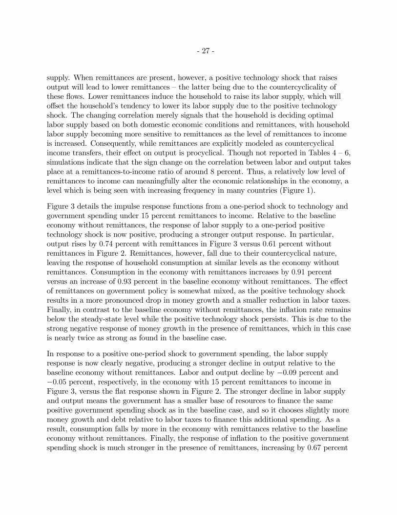
As shown in Figure 1, developing countries now receive remittances in significant amounts,with the top 20 remittance-dependent countries recording annual flows of between 7 and 27percent of GDP during 2003. Annual averages over the period 1990-2003 paint a similarpicture, as the top 20 developing countries received remittance flows between 4 and 18percent of GDP. The recipients of the largest remittance flows are India, Mexico, and thePhilippines, each of whom received between $7 and $14 billion in remittances during 2002.These three countries have been consistent recipients of remittances, recording the largestaverage annual flows between 1990 and 2002.5 As reported by IMF (2005b) and WorldBank (2006), the largest source of remittances is the United States and the two largest

4World Bank (2006). Remittances are defined in the broadest possible terms to include workers’ re-mittances, compensation of employees, and migrant transfers. Total worldwide remittances, which includeremittances to both developed and developing economies, were estimated at $232 billion in 2005. Remittancesto developing countries, therefore, constitute over 70 percent of total remittance flows.

5Many developed countries such as Spain and France also receive significant remittance inflows, but theseamounts are negligible in terms of GDP.

- 8 -

destination regions of remittance flows are Latin America and developing Asia. Thesestudies both indicate that remittance flows are beginning to outpace official transfers,private equity flows, and FDI. Across the Caribbean, for example, Mishra (2005) reportsthat remittances increased from 3 to 13 percent of GDP from 1990 to 2002, while FDI fellfrom 11 to 7 percent and ODA fell from 4 to 1 percent. Across all developing countries,IMF (2005b) reports that remittances are now the second largest inflow behind FDI, butahead of ODA and non-FDI private capital inflows.6 The need to understand the impact ofthese flows on economic decision making is readily apparent.

The existing literature on remittances has mainly focused on the motivation to remit andthe microeconomic implications of remittances. On the motivation for remittances, theliterature has been divided between those who argue that remittances are altruisticallymotivated and those who believe that remittances behave more like capital flows — that is,they are driven by selfish reasons and the remitter’s desire to invest in the home country.This latter approach has often been referred to as the portfolio motive behind remittancesand has been advanced in a variety of studies, including Straubhaar (1986), Elbadawi andRocha (1992), El-Sakka and McNabb (1999), and Buch, Kuckulenz, and Le Manchec(2002) to suggest that remittances promote development and enhance growthopportunities. The theory of altruistically motivated remittance flows is related to familyties in the home country and the desire of the remitter to provide resources and care forthose family members left behind. Altruistic motivations for remittances are discussed inLucas and Stark (1985), Chami, Fullenkamp, and Jahjah (2003, 2005), Gupta (2005), andWorld Bank (2006), and have their roots in Becker’s (1974) analysis on economics of thefamily. Lucas and Stark (1985) specify a utility function in which the remitter’s utilityincludes consumption of the remaining household members in the home country.Altruistically motivated remittance behavior is, therefore, consistent with existing theoryon altruistically motivated bequest behavior, where utility of the parents includes lifetimeresources of their children.

Establishing the primary motivation behind remittance behavior is important since thealtruistic and portfolio motives have different implications for the relationships betweenremittances, household decisions, and other economic variables of interest in the receivingcountry. For example, if remittance flows are primarily portfolio motivated, then one wouldexpect remittances, like investment, to be procyclical relative to output in the receivingcountry. However, if remittances were primarily motivated by altruistic behavior on thepart of the remitter, then remittances as compensatory income transfers would becountercyclical relative to output in the receiving country. The remitter would attempt to

6The dramatic growth in remittances may also simply reflect the concerted effort to bring these trans-actions into the formal transfer market as governments have intensified efforts to control money launderingand other potentially illicit transactions.

- 9 -

remit more when economic conditions were worsening in the home country and may remitless during economic expansions in the home country.

An examination of the existing econometric studies on remittance behavior suggests thatremittances are primarily motivated by altruism. Chami, Fullenkamp, and Jahjah (2003,2005) develop a model for examining the causes of remittances and, using cross-countrydata from 1970-98, find that remittances tend to be negatively correlated with GDPgrowth while capital flows such as FDI have a positive correlation. The authors concludethat remittances appear to be primarily intended to serve as compensation for pooreconomic performance in the home country. More recently, IMF (2005b) uses annual dataon a panel of 87 countries from 1980 to 2003, Mishra (2005) investigates data for 13Caribbean countries from 1980 to 2002, and World Bank (2006) examines cross-countrydata from 1995 to 2003. Like Chami, Fullenkamp, and Jahjah (2003, 2005), these studiesfind that remittances are countercyclical.7 Though these studies cite other factors asimportant determinants of remittances in addition to home country income, we focus onlyon the income of remittance recipients in the home country since it is instructive in themodel specification that follows.8 Inclusion of the remaining factors does not change thethrust of the present exercise. Therefore, although some support for the portfolio motivebehind remittance behavior exists (e.g., Lucas and Stark, 1985; and Mishra, 2005),altruism appears to dominate in a cross-country setting.

The literature, however, has largely been silent on the impact of countercyclical remittanceflows on government policy and the macro economy, especially in the context of a fullyspecified general equilibrium framework. Studies examining the macroeconomicimplications of remittances have instead relied on surveys of households in differentcountries. Recently, Adams (2004) uses household surveys to look at the role ofremittances in alleviating poverty in Guatemala while Amuedo-Dorantes, Bansak, andPozo (2005) examine remittance patterns from Mexico survey data. Finally, McKenzie(2005) investigates the impact of these flows on Mexican household decisions and allocationof resources.9 In contrast to the micro-based literature, the existing macroeconomic studiesdo not utilize an optimizing framework when examining the impact of remittances, whichhinders a systematic analysis of these flows. Thus, one of the main contributions of thispaper is to provide such a optimizing framework. We proceed in the next section by

7Additional single-country analysis by Gupta (2005) and Bouhga-Hagbe (2004) also lends empirical sup-port for the altruistic motive.

8Chami, Fullenkamp, and Jahjah. (2003, 2005), World Bank (2006), IMF (2005), and Bougha-Hagbe(2004), among others, indicate that other important determinants of remittances include the income of theremitter in the host country (proxied by the host country output), the degree of attachment to the familyand home country, and other demographic factors, including the number of years in host country.

9See also Lucas and Stark (1985) for remittances in Bostwana and Agarwal and Horowitz (2002) forremittances in Guyana.

- 10 -

developing a stochastic dynamic general equilibrium model with distortionary governmentpolicy in order to investigate the implication of countercyclical remittance flows oneconomic decision making and the conduct of monetary and fiscal policy in a business cyclesetting.

III. A STOCHASTIC MONETARY ECONOMY WITH REMITTANCES

The properties of remittances and their relation to optimal policies and allocations areexamined in a stochastic monetary economy. The model is a combination of acash-in-advance model and a stochastic growth model, similar to models employed inCooley and Hansen (1995), Chari, Christiano, and Kehoe (1991), and Lucas and Stokey(1983). The economy has a representative household, a representative firm, a government,and remitters. The household derives utility from leisure and two consumption goods, acash good and a credit good where previously accumulated cash balances are needed topurchase units of the cash good. Output is produced according to a production functionthat combines capital, labor, and technology, where the process governing technology isassumed to be exogenous and stochastic. Given the preponderance of evidence on thealtruistic motive for remitting, the household in this economy receives remittances whichare exogenously specified as countercyclical real income transfers. These transfers augmentthe income received from production.

The government raises revenue with distortionary effects to finance its exogenous stochasticspending using a tax on labor income, printing money, or debt issuance through one-periodreal bonds. The government, however, is unable to levy a direct tax on remittance incomeflows, an assumption which accords with evidence from various studies (e.g., World Bank2006, p. 93) which report that remittances are not typically taxed directly by governments.Finally, as in Lucas and Stokey (1983), Alvarez, Kehoe, and Neumeyer (2004) and others,this framework does not include a tax on capital and therefore avoids the well understoodproblems arising from capital taxation in representative agent models.10

Assumptions of a fixed capital stock and logarithmic preferences enable computation ofclosed form equilibrium solutions for the private sector given a particular governmentpolicy. The Ramsey equilibrium solves for optimal fiscal and monetary policy in the

10In addition to ruling out taxation of the pre-existing stock of capital, an assumed zero capital tax isalso justified by the well established result that tax rates on capital should be close to zero on average inthe context of representative agent models. For other work on optimal capital taxation in this setting, seeAtkinson (1971), Diamond (1973), Pestieau (1974), Atkinson and Sandmo (1980), Judd (1985), Chamley(1986), and Chari, Christiano, and Kehoe (1991, 1994). In the context of heterogeneous agents, however,a positive tax rate on capital has been found to be optimal. Auerbach and Kotlikoff (1987), for example,detail capital taxation in an overlapping generations setting, while Aiyagari (1995) shows how idiosyncraticrisk and borrowing constraints lead to positive capital taxes.

- 11 -

presence of remittances given the equilibrium behavior of the private sector. This Ramseyequilibrium may be reduced to four operator equations given the equilibrium behavior ofinterest and prices. The system is nonlinear, and therefore the projection method isapplied to solve for the four policy functions and conduct simulations. If the private sectoris made more complex, these four conditions would need to be augmented with equilibriumconditions for interest rates and prices. These additional conditions would limit theaccuracy of the projection method since additional equations would limit the number ofnodes the computer can solve. Finally, given a fixed capital stock, the model highlights thedistortionary effects of policy. The optimal government policy will account for its impacton interest rates, prices, and remittances as well as on the optimal behavior of thehousehold and firms.

A. Production

Aggregate output, Yt, is produced according to the following constant returns-to-scaleproduction function,

Yt = exp(θt)Hαt K

1−αt , 0 < α < 1, (1)

where Kt and Ht are the aggregate capital stock and labor supply, respectively, and θtrepresents the available technology. Technology is assumed to be the realization of anexogenous stochastic process and evolves according to the following law of motion,

θt = ρθθt−1 + θ,t, 0 < ρθ < 1. (2)

The random variable, θ,t, is normally distributed with mean zero and standard deviationσθ,t and the realization of θ,t is known to all agents at the beginning of period t. Therestriction in this paper on labor’s share of income below unity means labor supply isnonlinear and marginal product of labor is endogenous.11 As discussed in the proceedingsection, the solution procedure used in this analysis preserves the nonlinearity of the laborsupply function and associated Jensen’s inequality effects, thereby capturing the cost ofgovernment policy and its interaction with remittances through the endogeneity of themarginal product of labor.

Investment in physical capital in period t produces capital in period t + 1 according to,

Kt+1 = (1− δ)Kt + Xt, 0 < δ < 1, (3)

11The production function in equation (1) has meaningful implications which differ from similar recent workby Aiyagari and others (2002), Alvarez, Kehoe, and Neumeyer (2004), and Schmitt-Grohé and Uribe (2004).These authors set α = 1 in which results in an exogenous marginal product of labor equal to ∂Y/∂H = exp(θ).Setting 0 < α < 1 results in an endogenous marginal product of labor of ∂Y/∂H = f (α, exp(θ), H, K) .

- 12 -

where Xt is the level of investment in period t and δ is the rate of depreciation. The capitalstock is assumed to be fixed so that Xt = X = δK and firms are assumed to takedepreciation charges before taxes are applied at the household level. If firms were notallowed to take depreciation charges before taxes were applied, the government would findit optimal to tax inelastically supplied investment and use the proceeds to retire moneybalances. The representative firm seeks to maximize profit by choosing labor supplyresulting in the standard first-order conditions for the wage rate and rental rate on capital,adjusted for constant capital.

B. Households, Remittances, and the Government

The representative household obtains utility from consumption and leisure. Preferences aresummarized by the following utility function,

Et

∞Xt=0

βt [a logC1t + (1− a) logC2t − γHt] , (4)

where C1 is the cash good, C2 is the credit good, γ is a positive constant and 0 < β, a < 1.The specification of linear disutility of labor is derived from the assumptions that labor isindivisible and allocation of labor is determined by employment lotteries (Hansen, 1985;and Rogerson, 1988). The household enters period t with previously accumulated assetsequal to the stock of money holdings, Mt, and gross returns from government bonds,BtRt−1, where Bt is the stock of bonds and Rt−1 is the gross real interest rate.

Following the results of the empirical studies that show remittances to be countercyclical,the household receives remittances in the form of a compensatory income transfer equal to,

Remt = r0

µY

Yt

¶r1

, (5)

where Y is the steady-state level of output and r0 and r1 are positive constants. Theresponsiveness of remittances to the business cycle is determined by the parameter r1 andthe steady-state level of remittances is equal to r0. Since remittances are additionalhousehold income outside the production process and the capital stock is assumed to befixed, the remittance function above models remittances as a pure income transfer.

Previously accumulated assets, income from production, and remittance income are allused to finance household expenditures during the period. Entering the period, the currentshocks to the economy are revealed. As a result, households know the past and currentrealization of technology and government spending and form expectations over futurepossible values. After the shocks are revealed and expectations are formed, the household

- 13 -

then decides labor supply, receives remittances, chooses consumption of the cash and creditgoods, government bonds, and the amount of money to be carried into the next period.Overall, household allocations must satisfy the following budget constraint,

C1t + C2t +Md

t+1

Pt+ BL

t+1 ≤ (1− ατ t) (Yt −X) + Remt +Mt

Pt+ BL

t RLt−1, (6)

where Pt is the price level and τ t is the tax applied to labor income, αYt. Remittances arenot subject to taxation like labor income. The term Md

t+1 is the demand for moneybalances by the representative household to be used in the next period and is aggregatedacross households in relation to money supply in equilibrium. Previously accumulatedmoney balances are used to purchase the cash good in the current period and must alsosatisfy the cash-in-advance constraint,

PtC1t ≤Mt. (7)

Real government consumption, Gt, is assumed to follow an exogenous stochastic process.Government policy includes sequences of labor taxes and supplies of money and bondswhich must satisfy the following budget constraint,

Mt

Pt+ BtRt−1 = τ tα (Yt −X)−Gt + Bt+1 +

Mt+1

Pt, (8)

where the initial stocks of money, M0, and bonds, B0, are given. The money supply andgovernment spending in period t are assumed to grow at the rate exp(gt)− 1 andexp(µt+1)− 1, respectively. Thus, the level of government spending and money stock aredefined as,

Gt = exp(gt)Gt−1, (9)

Mt+1 = exp(µt+1)Mt. (10)

The random variable gt is assumed to evolve according to the following autoregressiveprocess,

gt = ρggt−1 + g,t, (11)

where g,t, is normally distributed with mean zero and standard deviation σg,t. Like theshock to technology, the realization of g,t is known to all at the beginning of period t. Theeconomywide resource constraint is,

C1t + C2t + X + Gt = Yt + Remt, (12)

which states that output from production plus remittances can be consumed by either

- 14 -

households or the government.

C. Solution to the Household Problem

The specification of log preferences causes income and substitution effects to cancel,allowing equilibrium remittances and household allocations to be characterized for a givenset of government policy. The closed-form solutions for consumption and the price level are,

C1t =(Yt + Remt −X −Gt)β

¡a

1−a¢exp(−µt+1)

1 + β¡

a1−a¢exp(−µt+1)

, (13)

C2t =(Yt + Remt −X −Gt)

1 + β¡

a1−a¢exp(−µt+1)

, (14)

Pt =Mt

(Yt + Remt −X −Gt)

"1 + β

¡a

1−a¢exp(−µt+1)

β¡

a1−a¢exp(−µt+1)

#. (15)

The closed-form solution for the interest rate is found by inserting (14) at time t and t + 1into

Rt =1

βC2t

⎡⎣ 1

Et

h1

C2t+1

i⎤⎦ , (16)

which is derived from the Euler condition on government bonds.

The solution for the credit good in (14) can also be used to solve for optimal labor supply,defining an implicit function,

Ht = h¡gt, θt, µt+1, τ t

¢. (17)

This equation cannot be solved for Ht explicitly, but the implicit function theorem allowsfor the construction of an implicit function which defines the explicit function. Definedderivatives can be obtained as long as an implicit function is known to exist under theimplicit function theorem. Since an implicit function for equilibrium labor can beconstructed,12 optimal household allocations and the equilibrium price system are allfunctions of contemporaneous government policy, the exogenous shocks to governmentspending and technology, and the level of remittances. It is clear from equations (17), (1),and (5) that the realization of exogenous shocks and government policy determines laborsupply, aggregate output, and aggregate remittances, respectively. Thus, while remittancesare not directly subject to government taxation, government policy indirectly influences the

12See Cosimano and Gapen (2005) for additional details.

- 15 -

level of remittances through changes in the marginal product of labor.

The equilibrium price system is dependent on past policy and expectations of future policy,remittances, and uncertainty. The price level is dependent on the choice of money balancesduring the previous period which is a result of the cash-in-advance specification.Consequently, the choice of money growth in period t by the government affects the pricelevel in period t and in period t + 1. The interest rate in period t is a function of theexpectation over future government policy, remittances, and labor supply decisions inperiod t+ 1 since the interest rate applied to the stock of bonds chosen by the household inperiod t will not be available for use again until period t + 1.

The stochastic monetary economy contains a loss function via the presence of nonlinearitiesin the labor supply equation since the contemporaneous tax on labor income and moneygrowth result in direct changes to household labor supply and additional indirect effectsthrough remittances and endogenous changes in the marginal product of labor.13 Takentogether, the direct and indirect effects jointly determine optimal household labor supply.14

Variations in government policy directly affect labor supply, output, remittances, remaininghousehold allocations, and the equilibrium price system while feeding back into thegovernment budget constraint through tax revenue. In addition, the shocks to technologyand government spending cause changes in remittances and induce responses by bothhouseholds and the government, thereby determining the overall volatility of the modeleconomy. Equilibrium decisions by households, firms, the government, and remitters arethen transmitted across time through the price level and interest rate. Thus, while optimallabor supply is only based on contemporaneous variables, the price system embedsexpectations over the future path of remittances, policy, and the possible realizations ofgovernment spending and technology shocks. The degree to which changes in remittances,government policy, or exogenous shocks offset or magnify distortionary effects onequilibrium allocations depends on the degree of countercyclicality of remittances and theamount of nonlinearity present within the system, and within the labor supply function inparticular.

IV. THE RAMSEY EQUILIBRIUM WITH REMITTANCES

The goal of the government is to maximize the welfare of the household subject to raising

13The preservation of nonlinearities in the labor supply equation (17) endogenizes the assumption of aloss function over distortionary taxes and inflation as discussed in Barro (1979), Barro and Gordon (1981),Bohn (1988), and Schmitt-Grohé and Uribe (2004). These authors use a quadratic loss function to capturethe excess burden of taxes and allocative distortions of inflation.14While debt is not explicitly present in the labor supply function, it still plays a role since the choices of

taxes and money determine the level of debt as a residual in the government budget constraint.

- 16 -

revenues through distortionary means. After the shocks to the system are revealed, thegovernment selects a policy profile and households respond with a set of allocations. Theresulting equilibrium determines the state variables for the next period. Therefore, whenchoosing an optimal policy mix, the government must take into account the equilibriumreactions by households, remitters, and firms to the chosen policy mix. The government isalso constrained in its policy choices since it must choose a policy mix to maximizehousehold utility while satisfying the government budget constraint. The followingdefinition describes the Ramsey equilibrium with remittances.

Definition 1. A feasible allocation is a sequence of {C1t}∞t=1, {C2t}∞t=1, {Ht}∞t=1, {Gt}∞t=1

that satisfy the resource constraint in (12). A price system is a set of nonnegative boundedsequences {Pt}∞t=1 and {Rt}∞t=1. A government policy is a set of sequences {τ t}

∞t=1,

{Mt+1}∞t=1, {Bt+1}∞t=1 .

Definition 2. Given the exogenous sequences {gt}∞t=1 and {θt}∞t=1; initial stocks of money

and bonds; and M0 = Md0 ; a competitive equilibrium is a feasible allocation, a price

system, and a government policy such that (a) given the price system and governmentpolicy, the allocation solves both the firm’s problem and the household’s problem; and (b)given the allocation and price system, the government policy satisfies the sequence ofgovernment budget constraints.

Definition 3. The Ramsey problem is to choose a competitive equilibrium that maximizeshousehold utility. The competitive equilibrium that solves the Ramsey problem is calledthe Ramsey plan or Ramsey equilibrium.

A. The Ramsey Problem

Under the assumption that an institution or commitment technology exists through whichthe government can bind itself to a particular sequence of policies, the governmentattempts to maximize household utility in (4) subject to the government budget constraintin (8) while taking into account the equilibrium specification for the price system andoptimal responses by households and firms.15 After the shocks to spending and technologyare realized, optimal policy is a mapping of state variables to labor taxes, money supply,and the amount of debt so that the government’s budget constraint is satisfied. Like the

15The Ramsey problem in the general equilibrium dynamic programming setting incorporates many of thereputational mechanisms for credible government policies as discussed in Ljungqvist and Sargent (2000). Ingeneral, the government would find it optimal to deviate from its original set of policies if allowed, and somemechanism, reputational or otherwise, is needed to ensure credibility of government policy.

- 17 -

household maximization problem, the government’s problem can be set up as a dynamicprogramming problem whereby the government seeks to maximize,

V (st) = Max∆t

(a logC1t + (1− a)C2t − γHt+

λgt³τ tα (Yt −X)−Gt + Bt+1 + Mt+1

Pt− Mt

Pt−BtRt−1

´+ βEtV (st+1)

)(18)

where ∆t = (τ t, µt+1, Bt+1) is the set of choice variables, st represents the set of statevariables

¡Bt, Md

t /Pt−1, θt−1, gt−1, τ t−1, Rt−1

¢, and λgt is the Lagrange multiplier on the

government budget constraint. The first-order conditions for the Ramsey problem are,16

τ t :

(aC1t

∂C1t

∂τ t+ 1−a

C2t

∂C2t

∂τ t− γ ∂Ht

∂τ t+

λgthατ t

∂Yt∂τ t

+ α (Yt −X)−Bt∂Rt−1

∂τ t−¡exp(µt+1)− 1

¢Mt

Pt1Pt

∂Pt∂τ t

i ) =

βEt

½λgt+1Bt+1

∂Rt

∂τ t

¾, (19)

µt+1 :

( aC1t

∂C1t

∂µt+1+ 1−a

C2t

∂C2t

∂µt+1− γ ∂Ht

∂µt+1+

λgthατ t

Yt∂µt+1

− Mt+1

Ptexp(µt+1)−Bt

∂Rt−1

∂µt+1−¡exp(µt+1)− 1

¢Mt

Pt1Pt

∂Pt∂µt+1

i ) =

βEt

½λgt+1Bt+1

∂Rt

∂µt+1

¾, (20)

Bt+1 : λgt = βEt {λgt+1Rt} , (21)

where λgt represents the marginal utility of relaxing the government budget constraint byone unit or, as suggested by Bohn (1988), the value that households place on the ability ofthe government to raise revenue from a source “outside” the economy. Such an abilitywould be equivalent to collection of a lump-sum tax, making the multiplier equal to thecost of distortionary government revenue policies.

Equations (19) and (20) reveal the importance of maintaining the endogeneity of thenonlinear labor supply function when examining the relationship between governmentpolicy and remittances. The impact of labor taxes and money growth on household welfareinclude both the direct effects of changes in government policy on labor supply and theindirect effects through changes in the endogenous marginal product of labor. For example,∂C1

∂τ=¡∂C1

∂Y∂Y∂H

+ ∂C1

∂Rem∂Rem∂Y

∂Y∂H

¢∂H∂τ

. The direct effect of policy on labor supply is containedin ∂H/∂τ and the indirect effect of policy on output and remittances is contained in the

16The first-order condition for money shown here is actually ∂/∂¡exp(−µt+1)

¢. This was done for

simplicity of computation. The optimal government policy for money balances can then be found bytaking the − log(x) of the result.

- 18 -

parenthetical term. Therefore, an accurate assessment of the relationship betweenremittances, government policy, and household decisions requires a solution procedure thatcaptures these direct and indirect effects. Preserving the endogenous properties of themarginal product of labor is also important in the determination of the variances andcovariances of the model economies during simulation.17

The Euler condition in (19) describes the trade-off between taxation and issuing debt. Thefirst terms on the left-hand side reflect the changes in consumption of the cash and creditgoods and provision of labor by the household from a change in taxes. A change in the taxrate enters consumption of the cash and credit good indirectly via the equilibrium laborcondition, which includes the impact of remittances. The bracketed term in (19) describesthe change in the government budget constraint from a change in taxes scaled by themultiplier. The first terms inside the bracket represent the direct change in tax revenuefrom a change in tax policy, the sign of which depends on the nonlinear response of laborsupply to a change in taxes. The remaining terms result from the commitment technologyand the price effect on nominal money balances. These combined effects must be equal tothe alternative policy of issuing additional debt which matures in the next period.

The trade-off between issuing money and debt is more complicated since money enters (20)directly through the money growth term and indirectly through the equilibrium laborcondition. The first terms on the left-hand side detail the effects of money growth onconsumption and labor supply, which depend on the net effect of money growth on outputand consumption versus money growth on remittances. The bracketed term, as in the taxcondition, details the impact of changes in money on the government budget constraintscaled by the multiplier, including the price effect on nominal variables. The first termdescribes the change in labor tax revenue based on the change in equilibrium labor fromchanges in money growth. These combined effects on the left-hand side must be equal tothe alternative policy of issuing debt which matures during the next period.

B. Calibration and Solution Procedure

The system of equations that characterize the optimal policies in the Ramsey equilibriumtheoretically is nonlinear. Therefore, the system is characterized quantitatively by assigningvalues to the parameters of technology, spending, preferences, and policy variables. Sincethe baseline economy contains no remittances, the process begins by calibrating the modelto a non-remittance-dependent economy. In this case, the model is calibrated to match the

17The use of linear labor supply and resulting exogenous indirect effects, as in Aiyagari and others (2002),Alvarez, Kehoe, and Neumeyer (2004), and Schmitt-Grohé and Uríbe (2004), eliminates an important chan-nel for optimal household decision making and the evaluation of the relationship between distortionarygovernment policy and remittances.

- 19 -

general features of the post-Korean War U.S. economy as reported in the U.S. NationalIncome and Product Accounts (NIPA).18 Though the United States is the largest sourcecountry of remittance flows, with $39 billion in outward remittances in 2004 (World Bank,2006), this total amounts to only 0.3 percent of GDP. Furthermore, a robust examinationof business cycle properties of the U.S. economy is readily available for comparisonpurposes (e.g., Cooley and Prescott, 1995; and Stock and Watson, 1999). The NIPA data isused to derive parameter values for the share of income attributable to capital and labor,the capital-output ratio, the fraction of time households spend working in the market, therelative importance of the cash good versus the credit good in the utility function,technology and spending shocks, and the ratio of government spending to output.19 Theparameter values are summarized in Table 1. Using quarterly data from 1990:1—2002:4 theratio of government spending to net national product was 18 percent and the ratio offederal government debt held by the public to net national product was 49 percent.20

The parameter describing the sensitivity of remittances to the business cycle is calibratedbased on the literature on bequest behavior found in the United States. Like remittances,bequests are private income transfers and altruism is a key motive that explains bequestbehavior (see Barro, 1974; and Becker, 1974).21 Altruism implies that parents bequeath ina compensatory fashion since they receive utility from the lifetime resources of theirchildren. A second implication of altruism is that parents will bequeath unequally,transferring more to children with fewer resources. Consequently, compensatory bequestbehavior mirrors the countercyclical remittance function in this paper and the empiricalfindings from the bequest literature can inform the calibration procedure. In this regard,Wilhelm (1996) uses data from the Estate-Income Tax Match data set to test severalaltruistic models of optimal bequest behavior and finds that a $1 increase in earnings of thedependent results in a reduction in bequests of between $0.12 and $0.19, depending on thebequest function tested.22 Based on the results of this study, the sensitivity of remittances

18This was done following the process in Stock and Watson (1999), Cooley and Prescott (1995), Cooleyand Hansen (1991, 1995), Hansen and Wright (1992), Christiano and Eichenbaum (1992), Chari, Christiano,and Kehoe (1991, 1994), Juster and Stafford (1991), and Hansen (1985).19A gross capital concept is assumed so that investment includes government investment. Government

spending is defined as net real government spending on goods and services, or real total government spendingless the sum of real defense investment, real non-defense investment, and real state and local investment.This amount is then taken as a ratio of real net national product.20The results in this paper were also solved and simulated under twice the current U.S. debt-to-GDP ratio.

The results were nearly identical to those presented here, suggesting the business cycle effects of remittancesare largely invariant to initial calibrated debt levels. However, as discussed below, the presence of remittanceslowers the marginal cost of government policy, meaning that additional debt may be easier to carry.21For arguments in favor of exchange-motivated bequests see Bernheim, Shleifer and Summers (1985). See

Perozek (1998) for a critique of the evidence on exchange motivation.22The Estate-Income Tax Match data set is especially useful since it contains reliable information on both

parents and heirs. The data set contains complete family information, matched by taxpayer identification

- 20 -

to the business cycle is set at r1 = 0.5, meaning that remittances, like bequests, arecompensatory on less than a one-to-one basis relative to output. In other words, a one unitincrease in real income relative to steady-state income results in a decline in remittances of0.05 units in equation (5). Our measure of the sensitivity of remittances to the businesscycle is therefore conservative, as the response is only about one-third to one-half thatsuggested by the altruistic bequest literature. Increasing this parameter would generallymagnify the business cycle results found herein, while a lower parameter value woulddampen the reported results.23

The steady-state level of remittances, r0, is varied from 5 to 30 percent of income duringthe solution and simulation procedure. This range was chosen to match data on meanworker remittances in percent of GDP for remittance-dependent economies as presented inFigure 1, and in other recent studies examining remittance flows such as World Bank(2006), Chami, Fullenkamp, and Jahjah (2003, 2005), Giuliano and Ruiz-Arranz (2005),and IMF (2005b). Thus, this range accurately describes the level of remittances found inwhat can be classified as “remittance-dependent” economies. Finally, the remainingvariables, γ and δ, are derived from first-order conditions and the non-stochasticsteady-state government budget constraint.24

The computational solution procedure is based on the projection approach as described byJudd (1992, 1998) and applied to Ramsey problems in Cosimano and Gapen (2005). Theset of Euler conditions from the Ramsey problem, the labor equation from the household’sproblem, and the government budget constraint yield a set of four operator equationsN (f) that define the Ramsey equilibrium with remittances. Since the set of operatorequations is nonlinear, the projection approach begins by defining the policy functions interms of polynomials. In this case, Chebyshev polynomials are used. The solution

numbers, and includes a variety of information in addition to income which is useful in controlling fornon-income related factors. See Wilhelm (1996) for additional information.23Another means of varying the sensitivity of remittances to the business cycle would be to alter the

functional form in equation (5). For example, Wilhelm (1996) tests several models of altruistic bequestmotives based on a linear specification, with the equivalent representation here similar to,

Remt = r0 + r1(Y − Yt),

with r0 defined as the steady-state level of remittances and r1 defined as in the text.24The non-stochastic steady-state values for taxes and depreciation used to calibrate the disutility of labor

are based on historical U.S. data, including the debt-to-income ratio. Re-calibration of the model undervarious levels of debt or remittances would result in different non-stochastic steady-state values for labortaxes and, in turn, the rate of depreciation and disutility of labor. In order to simulate each economy usingconstant household preferences, and therefore a constant baseline of preference parameters, the calibratedlevels of γ and δ are held constant at their U.S.-based levels without remittances across all model economiesin this analysis.

- 21 -

procedure solves for the optimal set of policies (Ht, µt+1, τ t, λgt) as functions of theexogenous shocks and state variables that set N (f) = 0 simultaneously and satisfy theRamsey equilibrium.25 Since the state vector is comprised of information known to allparties at the beginning of the period, the procedure can be viewed as choosing policyfunctions based on newly revealed information, namely the exogenous shocks to technologyand government spending, such that Euler and transversality conditions are satisfied.

The advantage of this approach is that the multiplier from the Ramsey problem, λg, isoptimally solved for as an endogenous policy variable. Since the projection method isdesigned to capture higher moments, this process will more accurately illustrate theproperties of the multiplier, the value of remittances, and the cost of distortionarygovernment policy. Consequently, the solution method applied in this paper differs fromother recent studies that use a simplified production function (Aiyagari and others, 2002;Alvarez, Kehoe, and Neumeyer, 2004; and Schmitt-Grohé and Uribe, 2004) or employ themore traditional primal approach (Chari, Christiano, and Kehoe, 1994; and Chari andKehoe, 1999).26 Once properly specified, the system is solved using a nonlinear equationoptimizer in Matlab. The results of this procedure are discussed in the next section.

V. RESULTS

The Ramsey problem was solved in economies with and without remittances. The baselineeconomy contains no remittances. When remittances are present, the solution was derivedunder various remittance-to-income ratios, ranging from 5 to 30 percent. Then using theoptimal coefficients of the polynomial approximations that describe the Ramsey plan, eacheconomy was simulated under the effects of technology and government spending shocks.

25The boundaries of the space defining the exogenous technology and government spending shocks arecalibrated from actual U.S. data. The interval for each is taken as a multiple of the standard deviationof the error process. Chebyshev collocation methods divide the state space over θ and g into discrete gridpoints, where higher numbers of points produce a more defined grid space for which the system is solvedover. The set of residual functions also contain conditional expectations which must be evaluated. Sincethe processes that govern the shocks to technology and government spending are assumed to be distributedN(0, σ2θ,g), expectations can be evaluated using Gauss-Hermite Quadrature. In this procedure, the form ofthe policy function is assumed to be independent of the realization of the shocks. Expectations are foundby integrating over the possible realizations of θ and g while treating the policy function as a constant.26The primal approach recasts the problem of choosing optimal policy as a problem of choosing allocations

subject to constraints which capture restrictions on those allocations. In practice this means using an infi-nite horizon budget constraint with prices and policy substituted out using first-order conditions, commonlyreferred to as the implementability constraint. The use of the implementability constraint often requires asearch procedure that iterates across candidate solutions for the multiplier (Chari, Christiano, and Eichen-baum, 1994) as opposed to endogenously solving for the multiplier as is done in this paper. Furthermore,the multiplier on the implementability constraint has a different interpretation than the multiplier in thispaper.

- 22 -

Statistics were computed by running multiple simulations of 5000 periods in length, takinglogarithms, and filtering each simulated time series using the H-P filter as described inHodrick and Prescott (1997).

A. Steady-State Decision Rules with Remittances

The upper panel in Table 2 represents the steady-state Ramsey equilibrium in levels orgrowth rates. In the baseline economy without remittances, optimal government policyfollows the Friedman rule by setting money growth equal to the rate of time preference.27

In this case, the Friedman rule results in an expected gross nominal interest rate equal to1.0 and the expected real return on money balances is equal to the inverse of timepreference in the steady state.28 In other words, the government equates the real gross rateof return on money balances and government debt in expectation, satisfying Eulerconditions. As discussed in Alvarez, Kehoe, and Neumeyer (2004) and Chari, Christiano,and Kehoe (1991, 1996), the Friedman rule is optimal in a variety of monetary economieswith distortionary taxes. That the government should avoid taxation of intermediategoods, in this case money balances, is also a well established result from public finance(e.g., Diamond and Mirrlees, 1971). Enacting the Friedman rule requires the government torun a gross-of-interest surplus by setting equilibrium labor income taxes high enough tocover government spending, interest on the debt, and the withdrawal of money balancesfrom the economy.

The existence of remittances provides the household with additional disposable income, andthe household spreads these resources over each of the consumption goods as well as leisure.Consequently, as remittances are added to the model economies, steady-state consumptionof the cash and credit goods increases while steady-state labor supply decreases. Forexample, Table 2 reports a decline in steady-state labor supply from 0.31 to 0.29, a declineof more than 6 percent, in the economy with a 5 percent remittance-to-income ratio. As theremittance-to-income ratio rises to 30 percent, steady-state labor supply declines by nearlya third and output falls by nearly 20 percent. Despite the decline in output as a result oflower steady-state labor supply, the household is able to increase overall consumption sincedisposable income — income from production plus remittances — has risen (Table 2).

27According to Friedman (1969), optimal monetary policy satiates the economy with real balances to theextent that it is possible to do so.28If the models in this paper included nominal government debt, the equilibrium nominal interest rate

would be equal to,

RNt =

1

β

1

Et

£exp−(µt+2)

¤ ,which would equal 1.0 if money supply grew at the rate of time preference, β.

- 23 -

As a result of adding remittances and their effect on labor supply and domestic output,optimal government policy responds by increasing steady-state taxes and money growth inorder to finance the same level of government spending and debt. The steady-state tax rateincreases from 18.8 percent in the economy without remittances to 21.1 percent under aremittances-to-income ratio of 30 percent. Over the same interval, the steady-state moneygrowth rate increases to 6 percent per quarter, indicating that optimal monetary policydeviates from the Friedman rule in the presence of remittances. Following the recent surveyby Kocherlakota (2005), non-optimality of the Friedman rule in a representative agentmodel with flexible prices is unusual. Reasons for the departure will be discussed morefully in the following sections. As these distortionary policy levers are increased, the cost ofgovernment policy increases at the margin, which would otherwise induce a further declinein steady-state labor supply in addition to the effect on labor from remittances. However,the presence of remittances insulates the household from distortionary government policyby providing a countercyclical source of income that government policy cannot act upondirectly. This is reflected through a lower value of the multiplier on the government budgetconstraint, which falls by nearly one-third as remittances are introduced. Although thegovernment needs to increase revenues through higher distortionary taxation and moneygrowth, the household is better able to absorb the additional distortion this policygenerates since fiscal and monetary policy act on a smaller portion of disposable income inthe presence of remittances.

B. Remittances and Business Cycle Moments

The bottom panel in Table 2 reports summary statistics on the moments of the businesscycle for each model economy. As is commonly found in most real business cycle models,the model without remittances generates about half of the standard deviation of output asfound in the U.S. economy.29 The model economy without remittances generates volatilityof consumption, prices, and inflation that more closely match features of U.S. data asreported in Stock and Watson (1999) and Cooley and Prescott (1995). Although moneysupply has very little volatility in the economy without remittances, volatility of the pricelevel and rate of inflation in each period are also determined by volatility of the cash gooddue to the cash-in-advance specification. The volatility of the interest rates is lower thanthat found in other studies since the values reported here are based on the filtered value ofthe gross interest rate series as opposed to a series of net interest rates. For reasonsdiscussed in the subsequent sections, however, the economies with remittances begin toapproach the level of volatility found in the U.S. economy.

29Stock and Watson (1999) report standard deviation of real GDP of 1.66 (from 1953—1996) and Cooleyand Prescott (1995) report standard deviation of real GNP of 1.72 percent (from 1954:1—1991:2). Some ofthe reduced model volatility is due to the assumption of a fixed capital stock since standard deviation ofinvestment is much higher than output and consumption.

- 24 -

The properties of each variable under each of the model simulations are displayed in Tables3 — 6. Table 3 contains the cross-correlation of each variable with output, governmentpolicy, and exogenous shocks for the economy without remittances and Tables 4 — 6 displaythe results with remittances. The model economy without remittances produces a negativecorrelation between labor and output, which stands in conflict with actual U.S. data.30

The negative correlation is a direct result of the assumption of a fixed capital stock,eliminating the complementary inputs characteristic of the production function.

The Baseline Economy without Remittances

This section details the response of government policy, household allocations, and pricesystem to a positive one-period shock to technology and government spending in theeconomy without remittances. The impulse response functions are displayed in Figure 2.31

The equilibrium response of household labor supply to a productivity shock is determinedby the combined effects of technology on the real wage, government policy, and themarginal utility of consumption. First, a positive shock to technology causes labor supplyto increase through the direct effect higher technology has on labor supply through ahigher real wage. The same increase in technology, however, also increases overall output.Since additional economywide resources are now available, government policymakers canreduce distortionary labor taxes and money growth and still finance the same level ofgovernment spending. This accounts for the negative correlation between technologyshocks and fiscal and monetary policy in Table 3. The reduction in the labor tax rate andmoney supply have positive correlations with labor supply that reinforce the direct effectfrom a higher after-tax real wage since decreases in taxes and money growth increase laborsupply. However, the increase in technology also decreases the marginal utility ofconsumption of the credit good, which otherwise causes a decrease in labor supply. Overall,these effects combine to produce a decline in labor supply.

In the baseline economy without remittances, a positive technology shock that causes a

30Cooley and Prescott (1995) report positive correlation between output and total hours of work andaverage weekly hours of work from using data from both the household survey and establishment survey.31Each set of vertical panels in the figure reports the percentage deviation from steady-state values for

the relevant variables under a positive one-standard deviation shock to technology (left vertical panels) andgovernment spending (right vertical panels). The percentage deviation of real and nominal interest ratesare based on gross rates. Deviation of money growth is based on the net money growth rate. The cross-correlations from the simulations in Tables 3 — 5 are based on filtered data as opposed to the impulse responsefunctions which are based on raw data. The use of the H-P filter generally reduces the persistence of thevarious series (i.e., reduces the tendency for the variables to remain away from their steady-state values) andoccasionally changes the sign of the initial response if the percentage deviation under raw data is very low.Nevertheless, this section proceeds with the standard use of raw data since the exercise remains illustrativeof model relationships.

- 25 -

decline in labor supply in the first period from its steady-state value produces a positivecorrelation between labor supply and government policy and a negative correlation betweenlabor supply and technology shocks, all of which are reported in Table 3. The household isable to spread the additional economywide resources across both consumption goods andincreased leisure since output rises even though labor supply falls. The government is alsoable to use the additional resources to pay down debt, although the percent deviation fromthe steady-state level of debt is small. The reduction in distortionary labor taxes andmonetary policy, along with slight declines in outstanding debt, result in a lower value forthe multiplier on the government budget constraint. In a situation where additionaleconomywide resources are available, the marginal cost of financing government spendinghas been reduced.

The effect of the positive shock to technology on prices is dependent on the change in thelevel of consumption of the cash good since the price level is determined through thecash-in-advance constraint which holds with equality in equilibrium. In this case, a higherlevel of cash good consumption lowers the period t price level relative to its steady-statevalue since nominal money balances were chosen during period t− 1 for use in period t.However, in periods t + 1 onward the positive technology shock results in higher inflationrelative to steady-state values since consumption of the cash good begins to return to itssteady-state level, or C1t+i+1 < C1t+i, and offsets the lower money growth rate.Consequently, the inflation dynamics in response to a positive technology shock first resultin lower inflation in the initial period of the shock and then slightly higher inflation relativeto steady-state inflation as the shock begins to expire. The real interest rate falls in periodt since the expected marginal value of consumption of the credit good in period t+ 1 is lessthan the level that prevails in period t as a result of the technology shock. The path thatconsumption of the credit good takes in return to the steady state, combined with Jensen’sinequality effects, results in a decline in real interest rates.

A positive shock to government spending is displayed in the right column of Figure 2. Inthis case, the shock causes labor supply to decrease through the direct effect of higher taxeson labor supply through a lower after-tax real wage. The increase in labor taxes, moneygrowth, and debt occur since policymakers need to finance the additional governmentspending, resulting in a positive correlation between government spending and labor taxes,money growth, and debt in the both panels of Table 3. The increase in the labor tax rateand money supply have a negative effect on labor supply that reinforces the direct effectfrom a lower after-tax real wage since increases in taxes and money growth decrease laborsupply through the implicit function governing labor supply. However, the increase ingovernment spending also increases the marginal utility of consumption of the credit good,which otherwise induces an increase in labor supply. In the baseline economy withoutremittances, these effects are largely offsetting, causing negligible declines in labor supplyand output. The resulting lack of correlation between shocks to government spending and

- 26 -

both labor supply and output in the baseline economy without remittances are reflected inTable 3.

Since output remains essentially flat, the increased government spending pullseconomywide resources away from the household, resulting in reduced consumption of bothcash and credit goods while leisure remains relatively unchanged. The increase indistortionary labor taxes and money growth, along with slight increases in outstandingdebt, result in a higher value for the multiplier on the government budget constraint. In asituation where additional government spending makes claims on an unchanged amount ofeconomywide resources, the marginal cost of financing government spending has increased.This is reflected in a higher value of the multiplier on the government budget constraintwhich increases 3 percent from its steady-state level in the same period as the positiveshock to government spending is revealed.

The positive shock to government spending displays the expected positive relationship onprices. A lower level of consumption of the cash good increases the period t price levelsince nominal money balances have already been chosen during the previous period. Incontrast to the positive technology shock, inflation remains above its steady-state levelwhile the government spending shock persists. From period t + 1 onward, C1t+i+1 > C1t+i

which otherwise reduces inflation, but this effect is offset by higher money growth leavinginflation slightly above steady-state inflation for the duration of the government spendingshock. The interest rate increases in period t since the expected value of consumption ofthe credit good in period t + 1 is more than the level that prevails in period t asconsumption begins to return to steady-state levels.

The Economies with Remittances

The response of government policy, household allocations, and price system to a positiveone-period shock to technology and government spending in the economies withremittances is displayed in Figure 3 and Tables 4 — 6. The main difference between theeconomies with remittances and the economy without remittances is the changingrelationship between labor and domestic output in the presence of remittances. Asremittances are added, the magnitude of the negative correlation between labor supply andoutput is reduced. Under 5 percent remittances to income, the correlation falls from −1 to−0.92. At the 15 percent level of remittances to income, the correlation between laborsupply and output changes sign with the correlation registering 0.50. Finally, at aremittances-to-income ratio of 30 percent, the correlation between labor and outputapproaches 1.0, a near complete reversal from the economy without remittances.

The simulation results indicate that, for the economy without remittances, a positivetechnology shock will lead to higher output, but will induce households to lower their labor

- 27 -

supply. When remittances are present, however, a positive technology shock that raisesoutput will lead to lower remittances — the latter being due to the countercyclicality ofthese flows. Lower remittances induce the household to raise its labor supply, which willoffset the household’s tendency to lower its labor supply due to the positive technologyshock. The changing correlation merely signals that the household is deciding optimallabor supply based on both domestic economic conditions and remittances, with householdlabor supply becoming more sensitive to remittances as the level of remittances to incomeis increased. Consequently, while remittances are explicitly modeled as countercyclicalincome transfers, their effect on output is procyclical. Though not reported in Tables 4 — 6,simulations indicate that the sign change on the correlation between labor and output takesplace at a remittances-to-income ratio of around 8 percent. Thus, a relatively low level ofremittances to income can meaningfully alter the economic relationships in the economy, alevel which is being seen with increasing frequency in many countries (Figure 1).

Figure 3 details the impulse response functions from a one-period shock to technology andgovernment spending under 15 percent remittances to income. Relative to the baselineeconomy without remittances, the response of labor supply to a one-period positivetechnology shock is now positive, producing a stronger output response. In particular,output rises by 0.74 percent with remittances in Figure 3 versus 0.61 percent withoutremittances in Figure 2. Remittances, however, fall due to their countercyclical nature,leaving the response of household consumption at similar levels as the economy withoutremittances. Consumption in the economy with remittances increases by 0.91 percentversus an increase of 0.93 percent in the baseline economy without remittances. The effectof remittances on government policy is somewhat mixed, as the positive technology shockresults in a more pronounced drop in money growth and a smaller reduction in labor taxes.Finally, in contrast to the baseline economy without remittances, the inflation rate remainsbelow the steady-state level while the positive technology shock persists. This is due to thestrong negative response of money growth in the presence of remittances, which in this caseis nearly twice as strong as found in the baseline case.

In response to a positive one-period shock to government spending, the labor supplyresponse is now clearly negative, producing a stronger decline in output relative to thebaseline economy without remittances. Labor and output decline by −0.09 percent and−0.05 percent, respectively, in the economy with 15 percent remittances to income inFigure 3, versus the flat response shown in Figure 2. The stronger decline in labor supplyand output means the government has a smaller base of resources to finance the samepositive government spending shock as in the baseline case, and so it chooses slightly moremoney growth and debt relative to labor taxes to finance this additional spending. As aresult, consumption falls by more in the economy with remittances relative to the baselineeconomy without remittances. Finally, the response of inflation to the positive governmentspending shock is much stronger in the presence of remittances, increasing by 0.67 percent

- 28 -

under 15 percent remittances to income versus 0.50 percent in the baseline economywithout remittances. The inflation rate remains well above the steady-state rate ofinflation as the positive government spending shock persists.

Since the correlation between labor and output has changed signs in the presence ofremittances, the correlation between labor and government policy has also changed signs.As can be seen from the simulation results in Tables 4 and 5, the correlation between laborsupply and labor taxes and money growth has changed from 0.34 and 0.53, respectively,under no remittances to −0.99 and −0.95, respectively, under a 15 percentremittances-to-income ratio. In fact, the sign change takes place at a slightly lower level ofremittances to income, as the correlation between labor supply and labor taxes is alreadynegative at 5 percent remittances to income. Fiscal and monetary policy have a strongernegative correlation with output in the economies with remittances relative to the baselineeconomy without remittances. Therefore, while their impact on output is procyclical,remittances serve to increase the countercyclicality of government policy.

The changing correlations between (i) labor supply and output and (ii) labor supply andlabor taxes in the presence of remittances are also behind the departure from optimality ofthe Friedman rule. As discussed in Alvarez, Kehoe, and Neumeyer (2004), the Friedmanrule of setting net nominal interest rates to zero is optimal under commitment when thegovernment has a sufficient number of independent policy instruments. In the baselineeconomy without remittances, the period t− 1 government has a sufficient number ofindependent instruments to bind and control the choices of the period t government. Byenacting the Friedman rule, the period t− 1 satiates consumers with real balances andequalizes expected rates of return across bonds and money. The period t− 1 government isleft with real bonds to induce the period t government to follow the same plan.

In contrast, the addition of remittances causes a reduction in labor supply and output,meaning the government has to raise additional resources, and following the Friedman rulein this case would require higher steady-state labor taxes to cover government spending,interest on the debt, and the withdrawal of money balances. Yet the changed correlationsbetween (i) labor supply and output and (ii) labor supply and labor taxes means followingthe Friedman rule would induce successive declines in labor supply and output, furtherincreasing remittance flows and creating further market inefficiencies. In other words andin the spirit of Tinbergen (1956), the changing correlations of underlying economicvariables in the presence of remittances means the government does not have a sufficientnumber of independent policy instruments to meet all of its objectives simultaneously.Consequently, the government finds it optimal to use its remaining policy instrument, theinflation tax or the nominal interest rate tax, as inflation is the return on nominal moneybalances, since the debt stock alone is not rich enough to adequately control the incentivesof successive governments.

- 29 -

One important conclusion that can be drawn from non-optimality of the Friedman rule inthe presence of remittances, therefore, is that the government needs to have a sufficientlyrich set of government policy instruments to carry out its policy plans. Remittances andthe need for instrument independence may be one reason why developing countries place agreater reliance on consumption-based taxation or implement financial transactions taxeslike those found in Colombia, Ecuador, and Brazil, among others. A consumption tax, orvalue-added tax, may be a more appropriate policy instrument since the tax could counterthe procyclical relationship between labor and output in the presence of remittances,providing more instrument independence relative to the labor income tax.

C. Remittances and Macroeconomic Risk

In the previous section, we detailed how the presence of remittances changes the sign of thecorrelation between labor and output from negative to positive as the household seeks tosmooth consumption. Alteration of the relationship between labor and output is significantfor a number of reasons. The surprising procyclical finding has the unsavory effect ofincreasing output risk, as seen by the increased volatility of output in the second panel inTable 2, and in Figure 4. Thus, remittances, while countercyclical, result in higher businesscycle volatility. Moreover, the increase in output risk will also produce an increase in laborsupply risk. Volatility of labor supply initially falls (Figure 4) as the correlation betweenlabor and output remains negative, but below unity. As additional remittances are added,the correlation switches sign and the positive correlation begins to increase labor supplyvolatility. Under higher levels of remittances, household labor supply is responding to thecombined effects of economic shocks on output and remittance flows, with the householdreacting more forcefully to the changes in remittances as the remittances-to-income ratioincreases. The increased volatility of labor supply will result in a more volatile process forreal wages and lead to increased labor market risk and, although not explicitly modeled inthis paper, will increase the importance of efficient wage contracting and risk-sharingbetween firms and households. This result is likely to be more pronounced when otherdistortions are introduced into the framework. For example, Chami and Fischer (2000) andChami, Fullenkamp, and Jahjah (2003, 2005), in the context of asymmetric information,find that such private income flows increase labor market risk.32

The impact of remittances on household consumption can also be seen by examiningFigure 4 and Table 2. First, remittances produce higher levels of disposable income and,

32Chami, Fullenkamp, and Jahjah (2003, 2005) introduce asymmetric information between the householdand the firms and between the household and the remitter. They show that profit maximization by risk-netural firms, in this case, induces these firms to shift more risk to the households. They conclude that theoptimal level of such transfers, which takes the firm’s need to break even into consideration, would result ina lower level of transfers being chosen than in the decentralized case.

- 30 -

consequently, higher steady-state consumption of cash and credit goods. However, thecountercyclical nature of remittances and their procyclical effect on output has offsettingeffects on the variability of consumption, with volatility of the credit good declining andvolatility of the cash good increasing. The ability of remittances to provide consumptioninsurance against shocks to household income therefore depends on the relative importanceof the cash and credit good in household consumption. The countercyclical nature ofremittances leads to an insurance effect on consumption of the credit good sinceremittances can be converted into the credit good in the same period the householdreceives the income transfer. Conversely, the cash-in-advance constraint means thehousehold has to transfer remittance resources across time to consume the cash good andthe more volatile inflation and output processes leads to increased volatility of cash goodconsumption. Since the calibrated values reported in Table 1 result in relative balancebetween the cash and credit good in household consumption, remittances are unable toreduce consumption volatility. Decreased volatility of credit good consumption is offset byincreased volatility of cash good consumption, leaving overall consumption volatilityunchanged.33 That said, overall consumption volatility that remains constant in the face ofincreasing business cycle volatility allows us to conclude that remittances do have aninsurance effect on consumption, if only to prevent consumption risk from increasing in linewith economywide output risk.

Like household consumption, the countercyclical nature of remittances and theirprocyclical effect on output has varying consequences on the volatility of governmentpolicy. In the economy without remittances, nearly all the volatility in government policyappears in labor taxes, as the labor tax rate fluctuates to preserve the Friedman rule(Figure 4 and Table 2). As remittances are added, the volatility of the labor tax ratedeclines, mirroring and contributing to the declining volatility of consumption of the creditgood. The presence of remittances increases the mean equilibrium growth rate of moneyand also increases its volatility. The increase in volatility of the money supply is acontributing factor to the increased volatility of the inflation process and consumption ofthe cash good. On balance, however, the cost of government policy appears to becomemore volatile as the standard deviation of the multiplier on the government budgetconstraint rises, contributing to an increase in policy risk.

D. Matching the Moments

While the goal of any real business cycle model is to match the moments of the model withactual data to examine the degree to which the model can explain observed economic

33Although not reported in Table 2, the standard deviation of total household consumption only falls from1.37 percent in the economy without remittances to 1.34 percent under a 30 percent remittances-to-incomeratio.

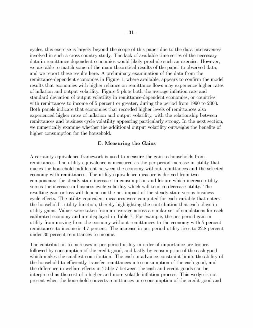
- 31 -

cycles, this exercise is largely beyond the scope of this paper due to the data intensivenessinvolved in such a cross-country study. The lack of available time series of the necessarydata in remittance-dependent economies would likely preclude such an exercise. However,we are able to match some of the main theoretical results of the paper to observed data,and we report these results here. A preliminary examination of the data from theremittance-dependent economies in Figure 1, where available, appears to confirm the modelresults that economies with higher reliance on remittance flows may experience higher ratesof inflation and output volatility. Figure 5 plots both the average inflation rate andstandard deviation of output volatility in remittance-dependent economies, or countrieswith remittances to income of 5 percent or greater, during the period from 1990 to 2003.Both panels indicate that economies that recorded higher levels of remittances alsoexperienced higher rates of inflation and output volatility, with the relationship betweenremittances and business cycle volatility appearing particularly strong. In the next section,we numerically examine whether the additional output volatility outweighs the benefits ofhigher consumption for the household.

E. Measuring the Gains

A certainty equivalence framework is used to measure the gain to households fromremittances. The utility equivalence is measured as the per-period increase in utility thatmakes the household indifferent between the economy without remittances and the selectedeconomy with remittances. The utility equivalence measure is derived from twocomponents: the steady-state increases in consumption and leisure which increase utilityversus the increase in business cycle volatility which will tend to decrease utility. Theresulting gain or loss will depend on the net impact of the steady-state versus businesscycle effects. The utility equivalent measures were computed for each variable that entersthe household’s utility function, thereby highlighting the contribution that each plays inutility gains. Values were taken from an average across a similar set of simulations for eachcalibrated economy and are displayed in Table 7. For example, the per period gain inutility from moving from the economy without remittances to the economy with 5 percentremittances to income is 4.7 percent. The increase in per period utility rises to 22.8 percentunder 30 percent remittances to income.

The contribution to increases in per-period utility in order of importance are leisure,followed by consumption of the credit good, and lastly by consumption of the cash goodwhich makes the smallest contribution. The cash-in-advance constraint limits the ability ofthe household to efficiently transfer remittances into consumption of the cash good, andthe difference in welfare effects in Table 7 between the cash and credit goods can beinterpreted as the cost of a higher and more volatile inflation process. This wedge is notpresent when the household converts remittances into consumption of the credit good and

- 32 -

leisure. Consequently, the household is better able to utilize the increase in householdresources and the countercyclical properties of remittances by transforming them intocontemporaneous consumption and leisure. Additional leisure represents nearly 60 percentof the overall increase in per period utility.

The gain in per period utility is mainly derived from the increased level effects in thesteady-state. While volatility of the economies with remittances is larger than the economywithout remittances, the cost of increased business cycle volatility is not sufficiently largeenough to offset the steady-state level effects on consumption and leisure. The simulationsindicate that the cost of increased business cycle volatility alone is equivalent to a presentdiscounted value of −0.7 percent of lifetime utility from moving from the economy withoutremittances to the economy with a 5 percent remittances-to-income ratio. This cost ofadditional output volatility from remittances is roughly equivalent in magnitude to the thecost of the business cycle volatility as reported by Lucas (1987, pp. 20-31). This cost,however, is much smaller than the 4.7 percent increase in per period utility from thesteady-state level effects on utility.

VI. CONCLUSION

Examination of external capital flows that are recorded in the capital account of thebalance of payments has been the subject of much interest by economists and researchers,especially following the Asian financial crisis of the 1990s. While the right mix of policiesto deal with volatile capital flows remains an open question, Calvo, Leiderman, andReinhart (1996) conclude that the developing economies that were most successful inmanaging the swings in capital flows relied on a comprehensive package of policy choices,as opposed to over reliance on a single instrument. Highly volatile international capitalflows and associated macroeconomic instability also caused many to question IMF policyrecommendations and the role of the IMF in capital account liberalization. In particular, inthe report on the IMF’s approach to capital account liberalization, the IndependentEvaluation Office of the IMF (IMF, 2005a, p. 5), concluded:

In encouraging capital account liberalization, the IMF pointed out the risksinherent in an open capital account as well as the need for a sound financialsystem, even from the beginning. The problem was that these risks wereinsufficiently highlighted, and the recognition of the risks and preconditions didnot translate into operational advice on pace and sequencing until later in the1990s (and even thereafter the policy advice has often been of limited practicalapplicability).

Remittances, which flow through the current account of the balance of payments, have not

- 33 -

received the same attention and careful scrutiny as private capital flows. In the absence ofa framework that allows for a systematic analysis of the impact of remittances on therecipient economy, a positive aura has surrounded and colored the role of remittances andthe policy prescription towards these flows. The conventional wisdom, with few exceptions,is that remittances: (i) represent a stable and reliable source of foreign exchange, (ii)reduce poverty, (iii) insure consumption against bad shocks, (iv) reduce macroeconomicvolatility, (v) enhance investment in physical and human capital, and (vi) alleviate creditconstraints. Consequently, there is a current emphasis among policymakers to highlightremittances as a potential cure to the many economic challenges facing developingcountries that depend on such transfers. Without careful analysis of the macroeconomicimplications of such transfers, policies aimed at encouraging remittances may createunintended consequences for the recipient economies.

This paper takes initial steps towards a unifying framework that assesses how remittancesinfluence the incentives and decisions of economic agents, while also investigating howthese decisions impact the recipient economy at large. The model applied is well groundedin the public finance and business cycle literature and relies on optimizing behavior byvarious agents in the economy. In this unifying framework we find that remittances, likeprivate capital flows, have both positive and negative economic effects. While remittancesincrease consumption and have the ability to smooth household consumption againstincome shocks, they may also contribute to increased macroeconomic risk through higherbusiness cycle volatility. The presence of remittances also changes the underlyingrelationship between labor and output, thereby changing the functioning of governmentpolicy instruments. If the set of policy instruments is not sufficiently varied, this mayresult in an increased reliance on the inflation tax.

We believe that the suggestion by Calvo, Leiderman, and Reinhart (1996) that governmentshould examine a wider variety of policy instruments when dealing with private capitalflows, should also apply to private income transfers such as remittances. We furtherencourage continued research into the macroeconomic effects of remittances, with particularemphasis on whether remittances entail additional economic and policy risk and, if so, towhat degree. We believe that our framework is general enough to allow for the addition ofother features that reflect particular institutional or country-specific factors. Finally, whileit is unlikely that remittances entail the same level of risk as private capital flows sinceremittances are generally altruistically motivated, we nevertheless hope that the analysispresented here can help formulate a well reasoned set of policy instruments and operationalguidance that can be provided to governments and policymakers faced with such flows.

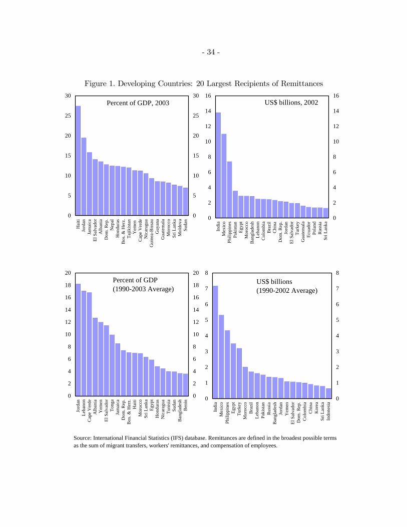
- 34 -

Figure 1. Developing Countries: 20 Largest Recipients of Remittances

Source: International Financial Statistics (IFS) database. Remittances are defined in the broadest possible terms as the sum of migrant transfers, workers' remittances, and compensation of employees.

0

5

10

15

20

25

30

Hai

tiJo

rdan

Jam

aica

El S

alva

dor

Alb

ania

Dom

. Rep

.N

epal

Hon

dura

sB

os. &

Her

z.Ta

jikis

tan

Yem

en

Cap

e V

erde

Nic

arag

uaG

uine

a-B

issa

uG

uyan

aG

uate

mal

aM

oroc

coSr

i Lan

kaM

oldo

vaSu

dan

0

5

10

15

20

25

30Percent of GDP, 2003

0

2

4

6

8

10

12

14

16

Indi

aM

exic

oPh

ilipp

ines

Paki

stan

Egyp

tM

oroc

coB

angl

ades

hLe

bano

nC

olom

bia

Bra

zil

Chi

naD

om. R

ep.

Jord

anEl

Sal

vado

rTu

rkey

Gua

tem

ala

Ecua

dor

Pola

ndR

ussi

aSr

i Lan

ka

0

2

4

6

8

10

12

14

16US$ billions, 2002

0

2

4

6

8

10

12

14

16

18

20

Jord

anLe

bano

nC

ape

Ver

deA

lban

iaY

emen

El S

alva

dor

Tong

aJa

mai

caD

om. R

ep.

Bos

. & H

erz.

Hai

tiM

oroc

coSr

i Lan

kaEg

ypt

Hon

dura

sN

icar

agua

Tuni

sia

Suda

nB

angl

ades

hB

enin

0

2

4

6

8

10

12

14

16

18

20Percent of GDP(1990-2003 Average)

0

1

2

3

4

5

6

7

8

Indi

aM

exic

oPh

ilipp

ines

Egyp

tTu

rkey

Mor

occo

Bra

zil

Leba

non

Paki

stan

Rus

sia

Ban

glad

esh

Jord

anY

emen

El S

alva

dor

Dom

. Rep

.C

olom

bia

Chi

naK

orea

Sri L

anka

Indo

nesi

a

0

1

2

3

4

5

6

7

8US$ billions (1990-2002 Average)

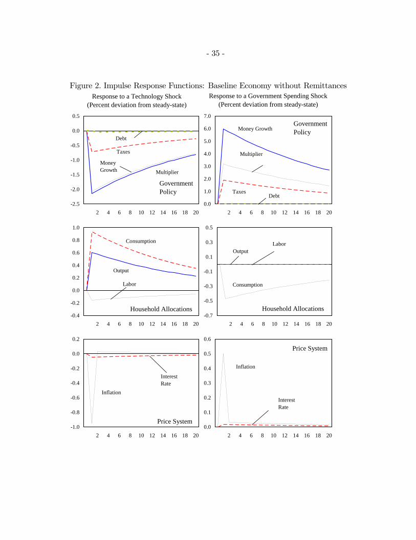
- 35 -

Figure 2. Impulse Response Functions: Baseline Economy without Remittances

Government Policy

Taxes

-2.5

-2.0

-1.5

-1.0

-0.5

0.0

0.5

2 4 6 8 10 12 14 16 18 20

Government Policy

TaxesDebt

0.0

1.0

2.0

3.0

4.0

5.0

6.0

7.0

2 4 6 8 10 12 14 16 18 20

Money Growth

Household Allocations-0.4

-0.2

0.0

0.2

0.4

0.6

0.8

1.0

2 4 6 8 10 12 14 16 18 20

Consumption

Output

Household Allocations-0.7

-0.5

-0.3

-0.1

0.1

0.3

0.5

2 4 6 8 10 12 14 16 18 20

Consumption

Price System-1.0

-0.8

-0.6

-0.4

-0.2

0.0

0.2

2 4 6 8 10 12 14 16 18 20

Inflation

Interest Rate

Price System

0.0

0.1

0.2

0.3

0.4

0.5

0.6

2 4 6 8 10 12 14 16 18 20

Inflation

Interest Rate

OutputLabor

Response to a Technology Shock(Percent deviation from steady-state)

Response to a Government Spending Shock(Percent deviation from steady-state)

Money Growth

Debt

Labor

Multiplier

Multiplier

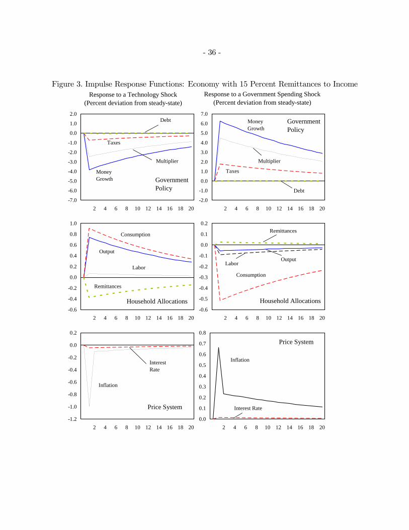
- 36 -

Figure 3. Impulse Response Functions: Economy with 15 Percent Remittances to Income

Government Policy

Taxes

-7.0

-6.0

-5.0

-4.0

-3.0

-2.0

-1.0

0.0

1.0

2.0

2 4 6 8 10 12 14 16 18 20

Government Policy

Taxes

Debt

-2.0

-1.0

0.0

1.0

2.0

3.0

4.0

5.0

6.0

7.0

2 4 6 8 10 12 14 16 18 20

Money Growth

Household Allocations-0.6

-0.4

-0.2

0.0

0.2

0.4

0.6

0.8

1.0

2 4 6 8 10 12 14 16 18 20

Consumption

Output

Household Allocations-0.6

-0.5

-0.4

-0.3

-0.2

-0.1

0.0

0.1

0.2

2 4 6 8 10 12 14 16 18 20

Consumption

Remittances

Price System

-1.2

-1.0

-0.8

-0.6

-0.4

-0.2

0.0

0.2

2 4 6 8 10 12 14 16 18 20

Inflation

Interest Rate

Price System

0.0

0.1

0.2

0.3

0.4

0.5

0.6

0.7

0.8

2 4 6 8 10 12 14 16 18 20

Inflation

Interest Rate

OutputLabor

Response to a Technology Shock(Percent deviation from steady-state)

Response to a Government Spending Shock(Percent deviation from steady-state)

Money Growth

Debt

Labor

Multiplier Multiplier

Remittances

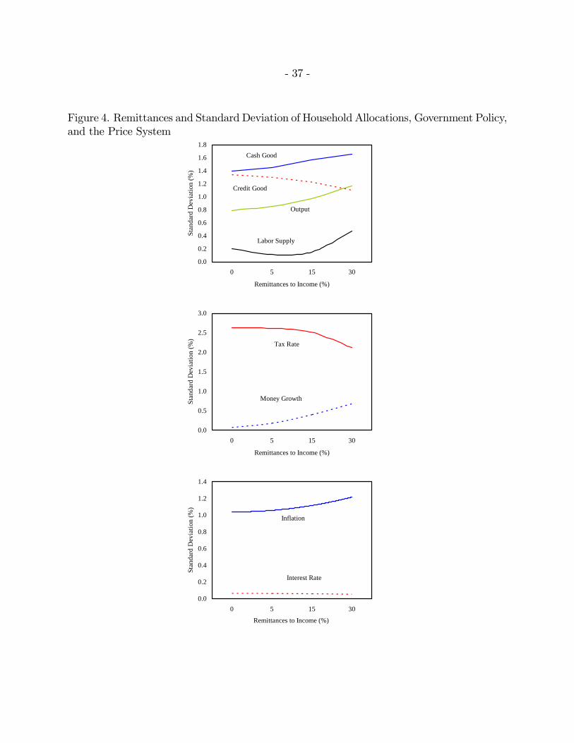
- 37 -

Figure 4. Remittances and Standard Deviation of Household Allocations, Government Policy,and the Price System

0.0

0.2

0.4

0.6

0.8

1.0

1.2

1.4

1.6

1.8

0 5 15 30

Remittances to Income (%)

Stan

dard

Dev

iatio

n (%

)

Cash Good

Credit Good

Output

Labor Supply

0.0

0.5

1.0

1.5

2.0

2.5

3.0

0 5 15 30

Remittances to Income (%)

Stan

dard

Dev

iatio

n (%

)

Tax Rate

Money Growth

0.0

0.2

0.4

0.6

0.8

1.0

1.2

1.4

0 5 15 30

Remittances to Income (%)

Stan

dard

Dev

iatio

n (%

)

Inflation

Interest Rate

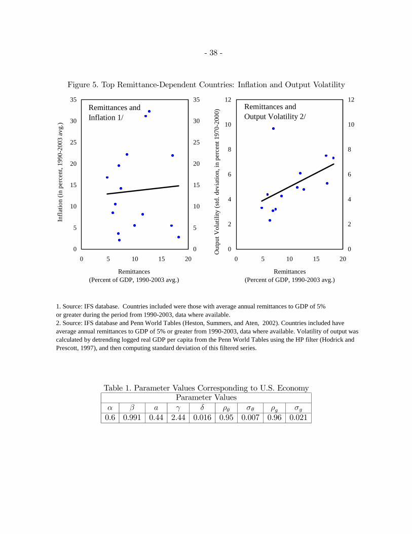
- 38 -

Figure 5. Top Remittance-Dependent Countries: Inflation and Output Volatility

0

5

10

15

20

25

30

35

0 5 10 15 200

5

10

15

20

25

30

35

0

2

4

6

8

10

12

0 5 10 15 200

2

4

6

8

10

12Remittances and Inflation 1/

Remittances and Output Volatility 2/

1. Source: IFS database. Countries included were those with average annual remittances to GDP of 5% or greater during the period from 1990-2003, data where available. 2. Source: IFS database and Penn World Tables (Heston, Summers, and Aten, 2002). Countries included haveaverage annual remittances to GDP of 5% or greater from 1990-2003, data where available. Volatility of output was calculated by detrending logged real GDP per capita from the Penn World Tables using the HP filter (Hodrick and Prescott, 1997), and then computing standard deviation of this filtered series.

Infla

tion

(in p

erce

nt, 1

990-

2003

avg

.)

Remittances (Percent of GDP, 1990-2003 avg.)

Remittances (Percent of GDP, 1990-2003 avg.)

Out

put V

olat

ility

(std

. dev

iatio

n, in

per

cent

197

0-20

00)

Table 1. Parameter Values Corresponding to U.S. EconomyParameter Values

α β a γ δ ρθ σθ ρg σg0.6 0.991 0.44 2.44 0.016 0.95 0.007 0.96 0.021

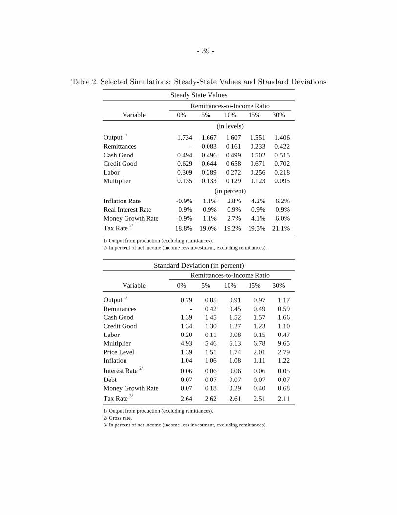
- 39 -

Table 2. Selected Simulations: Steady-State Values and Standard Deviations

Variable 0% 5% 10% 15% 30%

Output 1/ 1.734 1.667 1.607 1.551 1.406Remittances - 0.083 0.161 0.233 0.422Cash Good 0.494 0.496 0.499 0.502 0.515Credit Good 0.629 0.644 0.658 0.671 0.702Labor 0.309 0.289 0.272 0.256 0.218Multiplier 0.135 0.133 0.129 0.123 0.095

Inflation Rate -0.9% 1.1% 2.8% 4.2% 6.2%Real Interest Rate 0.9% 0.9% 0.9% 0.9% 0.9%Money Growth Rate -0.9% 1.1% 2.7% 4.1% 6.0%Tax Rate 2/ 18.8% 19.0% 19.2% 19.5% 21.1%

1/ Output from production (excluding remittances).2/ In percent of net income (income less investment, excluding remittances).

Variable 0% 5% 10% 15% 30%

Output 1/ 0.79 0.85 0.91 0.97 1.17Remittances - 0.42 0.45 0.49 0.59Cash Good 1.39 1.45 1.52 1.57 1.66Credit Good 1.34 1.30 1.27 1.23 1.10Labor 0.20 0.11 0.08 0.15 0.47Multiplier 4.93 5.46 6.13 6.78 9.65Price Level 1.39 1.51 1.74 2.01 2.79Inflation 1.04 1.06 1.08 1.11 1.22Interest Rate 2/ 0.06 0.06 0.06 0.06 0.05Debt 0.07 0.07 0.07 0.07 0.07Money Growth Rate 0.07 0.18 0.29 0.40 0.68Tax Rate 3/ 2.64 2.62 2.61 2.51 2.11

1/ Output from production (excluding remittances).2/ Gross rate.3/ In percent of net income (income less investment, excluding remittances).

Steady State Values

Remittances-to-Income RatioStandard Deviation (in percent)

Remittances-to-Income Ratio

(in levels)

(in percent)

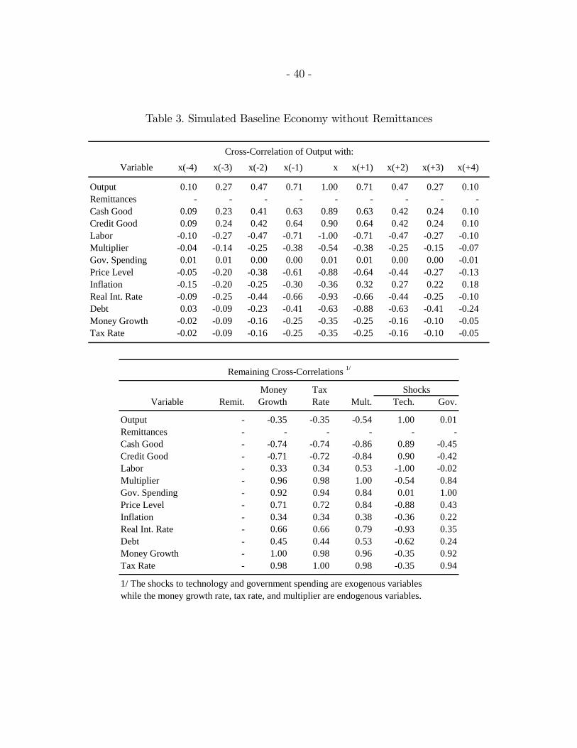
- 40 -

Table 3. Simulated Baseline Economy without Remittances

Variable x(-4) x(-3) x(-2) x(-1) x x(+1) x(+2) x(+3) x(+4)

Output 0.10 0.27 0.47 0.71 1.00 0.71 0.47 0.27 0.10Remittances - - - - - - - - -Cash Good 0.09 0.23 0.41 0.63 0.89 0.63 0.42 0.24 0.10Credit Good 0.09 0.24 0.42 0.64 0.90 0.64 0.42 0.24 0.10Labor -0.10 -0.27 -0.47 -0.71 -1.00 -0.71 -0.47 -0.27 -0.10Multiplier -0.04 -0.14 -0.25 -0.38 -0.54 -0.38 -0.25 -0.15 -0.07Gov. Spending 0.01 0.01 0.00 0.00 0.01 0.01 0.00 0.00 -0.01Price Level -0.05 -0.20 -0.38 -0.61 -0.88 -0.64 -0.44 -0.27 -0.13Inflation -0.15 -0.20 -0.25 -0.30 -0.36 0.32 0.27 0.22 0.18Real Int. Rate -0.09 -0.25 -0.44 -0.66 -0.93 -0.66 -0.44 -0.25 -0.10Debt 0.03 -0.09 -0.23 -0.41 -0.63 -0.88 -0.63 -0.41 -0.24Money Growth -0.02 -0.09 -0.16 -0.25 -0.35 -0.25 -0.16 -0.10 -0.05Tax Rate -0.02 -0.09 -0.16 -0.25 -0.35 -0.25 -0.16 -0.10 -0.05

Cross-Correlation of Output with:

Money Tax Variable Remit. Growth Rate Mult. Tech. Gov.

Output - -0.35 -0.35 -0.54 1.00 0.01Remittances - - - - - -Cash Good - -0.74 -0.74 -0.86 0.89 -0.45Credit Good - -0.71 -0.72 -0.84 0.90 -0.42Labor - 0.33 0.34 0.53 -1.00 -0.02Multiplier - 0.96 0.98 1.00 -0.54 0.84Gov. Spending - 0.92 0.94 0.84 0.01 1.00Price Level - 0.71 0.72 0.84 -0.88 0.43Inflation - 0.34 0.34 0.38 -0.36 0.22Real Int. Rate - 0.66 0.66 0.79 -0.93 0.35Debt - 0.45 0.44 0.53 -0.62 0.24Money Growth - 1.00 0.98 0.96 -0.35 0.92Tax Rate - 0.98 1.00 0.98 -0.35 0.94

1/ The shocks to technology and government spending are exogenous variableswhile the money growth rate, tax rate, and multiplier are endogenous variables.

Shocks

Remaining Cross-Correlations 1/

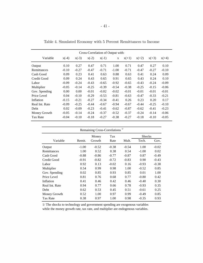
- 41 -

Table 4. Simulated Economy with 5 Percent Remittances to Income

Variable x(-4) x(-3) x(-2) x(-1) x x(+1) x(+2) x(+3) x(+4)

Output 0.10 0.27 0.47 0.71 1.00 0.71 0.47 0.27 0.10Remittances -0.10 -0.27 -0.47 -0.71 -1.00 -0.71 -0.47 -0.27 -0.10Cash Good 0.09 0.23 0.41 0.63 0.88 0.63 0.41 0.24 0.09Credit Good 0.09 0.24 0.43 0.65 0.91 0.65 0.43 0.24 0.10Labor -0.09 -0.24 -0.43 -0.65 -0.92 -0.65 -0.43 -0.24 -0.09Multiplier -0.05 -0.14 -0.25 -0.39 -0.54 -0.38 -0.25 -0.15 -0.06Gov. Spending 0.00 0.00 -0.01 -0.02 -0.02 -0.01 -0.01 -0.01 -0.01Price Level 0.04 -0.10 -0.29 -0.53 -0.81 -0.63 -0.47 -0.33 -0.21Inflation -0.15 -0.21 -0.27 -0.34 -0.41 0.26 0.23 0.20 0.17Real Int. Rate -0.09 -0.25 -0.44 -0.67 -0.94 -0.67 -0.44 -0.25 -0.10Debt 0.02 -0.09 -0.23 -0.41 -0.62 -0.87 -0.62 -0.41 -0.23Money Growth -0.05 -0.14 -0.24 -0.37 -0.52 -0.37 -0.24 -0.14 -0.06Tax Rate -0.04 -0.10 -0.18 -0.27 -0.38 -0.27 -0.18 -0.10 -0.05

Cross-Correlation of Output with:

Money Tax Variable Remit. Growth Rate Mult. Tech. Gov.

Output -1.00 -0.52 -0.38 -0.54 1.00 -0.02Remittances 1.00 0.52 0.38 0.54 -1.00 0.02Cash Good -0.88 -0.86 -0.77 -0.87 0.87 -0.49Credit Good -0.91 -0.82 -0.72 -0.83 0.90 -0.43Labor 0.92 0.13 -0.02 0.16 -0.93 -0.38Multiplier 0.54 0.99 0.98 1.00 -0.52 0.85Gov. Spending 0.02 0.85 0.93 0.85 0.01 1.00Price Level 0.81 0.76 0.68 0.77 -0.80 0.42Inflation 0.41 0.46 0.42 0.46 -0.40 0.30Real Int. Rate 0.94 0.77 0.66 0.78 -0.93 0.35Debt 0.62 0.53 0.45 0.51 -0.61 0.25Money Growth 0.52 1.00 0.97 0.99 -0.49 0.85Tax Rate 0.38 0.97 1.00 0.98 -0.35 0.93

1/ The shocks to technology and government spending are exogenous variableswhile the money growth rate, tax rate, and multiplier are endogenous variables.

Remaining Cross-Correlations 1/

Shocks

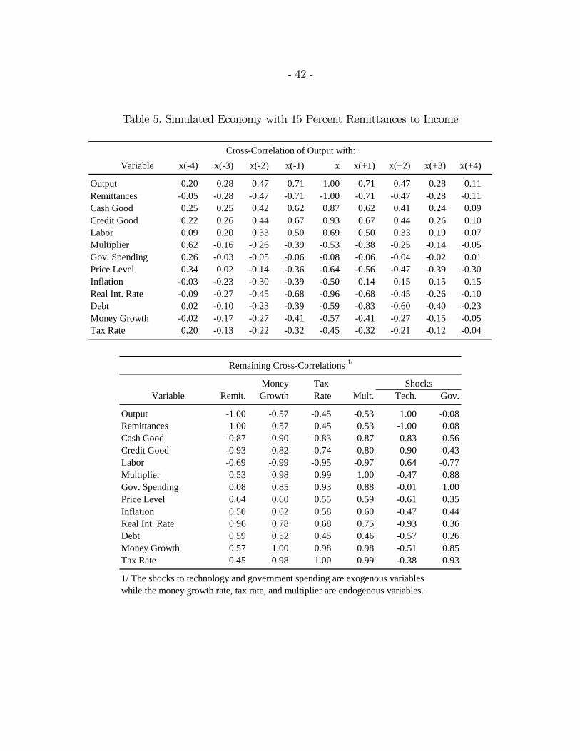
- 42 -

Table 5. Simulated Economy with 15 Percent Remittances to Income

Variable x(-4) x(-3) x(-2) x(-1) x x(+1) x(+2) x(+3) x(+4)

Output 0.20 0.28 0.47 0.71 1.00 0.71 0.47 0.28 0.11Remittances -0.05 -0.28 -0.47 -0.71 -1.00 -0.71 -0.47 -0.28 -0.11Cash Good 0.25 0.25 0.42 0.62 0.87 0.62 0.41 0.24 0.09Credit Good 0.22 0.26 0.44 0.67 0.93 0.67 0.44 0.26 0.10Labor 0.09 0.20 0.33 0.50 0.69 0.50 0.33 0.19 0.07Multiplier 0.62 -0.16 -0.26 -0.39 -0.53 -0.38 -0.25 -0.14 -0.05Gov. Spending 0.26 -0.03 -0.05 -0.06 -0.08 -0.06 -0.04 -0.02 0.01Price Level 0.34 0.02 -0.14 -0.36 -0.64 -0.56 -0.47 -0.39 -0.30Inflation -0.03 -0.23 -0.30 -0.39 -0.50 0.14 0.15 0.15 0.15Real Int. Rate -0.09 -0.27 -0.45 -0.68 -0.96 -0.68 -0.45 -0.26 -0.10Debt 0.02 -0.10 -0.23 -0.39 -0.59 -0.83 -0.60 -0.40 -0.23Money Growth -0.02 -0.17 -0.27 -0.41 -0.57 -0.41 -0.27 -0.15 -0.05Tax Rate 0.20 -0.13 -0.22 -0.32 -0.45 -0.32 -0.21 -0.12 -0.04

Cross-Correlation of Output with:

Money Tax Variable Remit. Growth Rate Mult. Tech. Gov.

Output -1.00 -0.57 -0.45 -0.53 1.00 -0.08Remittances 1.00 0.57 0.45 0.53 -1.00 0.08Cash Good -0.87 -0.90 -0.83 -0.87 0.83 -0.56Credit Good -0.93 -0.82 -0.74 -0.80 0.90 -0.43Labor -0.69 -0.99 -0.95 -0.97 0.64 -0.77Multiplier 0.53 0.98 0.99 1.00 -0.47 0.88Gov. Spending 0.08 0.85 0.93 0.88 -0.01 1.00Price Level 0.64 0.60 0.55 0.59 -0.61 0.35Inflation 0.50 0.62 0.58 0.60 -0.47 0.44Real Int. Rate 0.96 0.78 0.68 0.75 -0.93 0.36Debt 0.59 0.52 0.45 0.46 -0.57 0.26Money Growth 0.57 1.00 0.98 0.98 -0.51 0.85Tax Rate 0.45 0.98 1.00 0.99 -0.38 0.93

1/ The shocks to technology and government spending are exogenous variableswhile the money growth rate, tax rate, and multiplier are endogenous variables.

Remaining Cross-Correlations 1/

Shocks

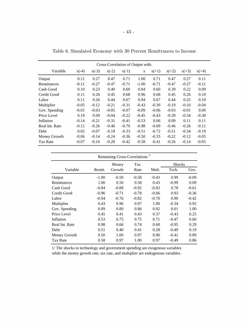
- 43 -

Table 6. Simulated Economy with 30 Percent Remittances to Income

Variable x(-4) x(-3) x(-2) x(-1) x x(+1) x(+2) x(+3) x(+4)

Output 0.11 0.27 0.47 0.71 1.00 0.71 0.47 0.27 0.11Remittances -0.11 -0.27 -0.47 -0.71 -1.00 -0.71 -0.47 -0.27 -0.11Cash Good 0.10 0.23 0.40 0.60 0.84 0.60 0.39 0.22 0.09Credit Good 0.11 0.26 0.45 0.68 0.96 0.68 0.45 0.26 0.10Labor 0.11 0.26 0.44 0.67 0.94 0.67 0.44 0.25 0.10Multiplier -0.05 -0.12 -0.21 -0.31 -0.43 -0.30 -0.19 -0.10 -0.04Gov. Spending -0.01 -0.03 -0.05 -0.07 -0.09 -0.06 -0.03 -0.01 0.00Price Level 0.19 0.09 -0.04 -0.22 -0.45 -0.43 -0.39 -0.34 -0.30Inflation -0.14 -0.21 -0.31 -0.41 -0.53 0.06 0.09 0.11 0.11Real Int. Rate -0.11 -0.26 -0.46 -0.70 -0.98 -0.69 -0.46 -0.26 -0.11Debt 0.02 -0.07 -0.18 -0.33 -0.51 -0.72 -0.51 -0.34 -0.19Money Growth -0.06 -0.14 -0.24 -0.36 -0.50 -0.35 -0.22 -0.12 -0.05Tax Rate -0.07 -0.16 -0.28 -0.42 -0.58 -0.41 -0.26 -0.14 -0.05

Cross-Correlation of Output with:

Money Tax Variable Remit. Growth Rate Mult. Tech. Gov.

Output -1.00 -0.50 -0.58 -0.43 0.99 -0.09Remittances 1.00 0.50 0.58 0.43 -0.99 0.09Cash Good -0.84 -0.89 -0.92 -0.83 0.78 -0.61Credit Good -0.96 -0.71 -0.78 -0.66 0.93 -0.36Labor -0.94 -0.76 -0.82 -0.70 0.90 -0.42Multiplier 0.43 0.96 0.97 1.00 -0.34 0.92Gov. Spending 0.09 0.89 0.86 0.92 0.01 1.00Price Level 0.45 0.41 0.43 0.37 -0.43 0.25Inflation 0.53 0.75 0.75 0.71 -0.47 0.60Real Int. Rate 0.98 0.66 0.74 0.60 -0.95 0.29Debt 0.51 0.40 0.41 0.28 -0.49 0.19Money Growth 0.50 1.00 0.97 0.96 -0.41 0.89Tax Rate 0.58 0.97 1.00 0.97 -0.49 0.86

1/ The shocks to technology and government spending are exogenous variableswhile the money growth rate, tax rate, and multiplier are endogenous variables.

Remaining Cross-Correlations 1/

Shocks

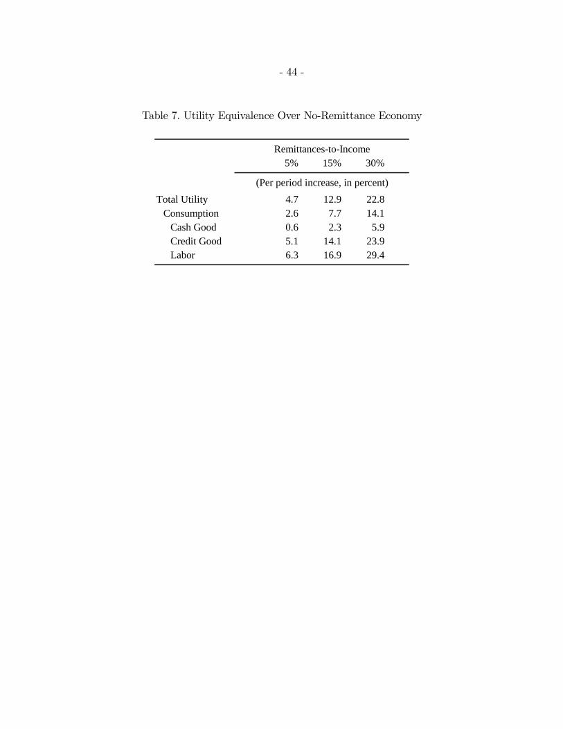
- 44 -

Table 7. Utility Equivalence Over No-Remittance Economy

5% 15% 30%

Total Utility 4.7 12.9 22.8Consumption 2.6 7.7 14.1

Cash Good 0.6 2.3 5.9Credit Good 5.1 14.1 23.9Labor 6.3 16.9 29.4

(Per period increase, in percent)

Remittances-to-Income

- 45 -

References

Adams, Jr., Richard H, 2004, “Remittances and Poverty in Guatemala,” World BankPolicy Research Working Paper No. 3418 (Washington: World Bank).

Agarwal, Reena, and Andrew W. Horowitz, 2002, “Are International Remittances Altruismor Insurance? Evidence from Guyana Using Multiple-Migrant Households,” WorldDevelopment, Vol. 30, pp. 2033-44.

Aiyagari, S. Rao, 1995, “Optimal Capital Income Taxation with Incomplete Markets,Borrowing Constraints and Constant Discounting,” Journal of Political Economy, Vol.106, pp. 1158-75.

Aiyagari, S. Rao, Albert Marcet, Thomas J. Sargent, and Juha Seppala, 2002, “OptimalTaxation without State-Contingent Debt,” Journal of Political Economy, Vol. 110,1220-54.

Alvarez, Fernando, Patrick J. Kehoe, and Pablo Andrés Neumeyer, 2004, “The TimeConsistency of Optimal Monetary and Fiscal Policies,” Econometrica, Vol. 72, pp.541-67.

Amuedo-Dorantes, Catalina, Cynthia Bansak, and Susan Pozo, 2005, “On the RemittingPatterns of Immigrants: Evidence from Mexican Survey Data,” Economic Review,Federal Reserve Bank of Atlanta, pp. 37-58.

Atkinson, A. B, 1971, “Capital Taxes, the Redistribution of Wealth and IndividualSavings,” Review of Economic Studies, Vo. 38, pp. 209-27.

, and A. Sandmo, 1980, “Welfare Implications of the Taxation of Savings,”Economic Journal, Vol. 90, pp. 529-49.

Auerbach, A., and Kotlikoff, L., 1987, Dynamic Fiscal Policy (Cambridge: CambridgeUniversity Press).

Barro, Robert J., 1974, “Are Government Bonds Net Wealth?” Journal of PoliticalEconomy, Vol. 82, pp. 1095-117.

, 1979, “On the Determination of the Public Debt,” Journal of Political Economy,Vol. 87, pp. 940-71.

, and David B. Gordon, 1981, “A Positive Theory of Monetary Policy in a NaturalRate Model,” Journal of Political Economy, Vol. 91, 589-610.

Becker, Gary, 1974, “A Theory of Social Interaction,” Journal of Political Economy, Vol.82, pp. 1063-93.

- 46 -

Bernheim, B. Douglas, Andrei Shleifer, and Lawrence H. Summers, 1985, “The StrategicBequest Motive,” Journal of Political Economy, Vol. 93, 1045-76.

Bohn, Henning, 1988, “Why Do We Have Nominal Government Debt?” Journal ofMonetary Economics, Vol. 21, pp. 127-40.

Bosworth, Barry P. and Susan M. Collins, 1999, “Capital Flows to Developing Economies:Implications for Saving and Investment,” Brookings Papers on Economic Activity, Vol.1, 143-80.

Bouhga-Hagbe, Jacques, 2004, “A Theory of Workers’ Remittances with an Application toMorocco,” IMF Working Paper 04/194 (Washington: International Monetary Fund).

Buch, Claudia M., Anja Kuckulenz, and Marie-Helene Le Manchec, 2002, “WorkerRemittances and Capital Flows,” Kiel Working Paper 1130 (Kiel: Kiel Institute forWorld Economics).

Calvo, Guillermo A., Leonardo Leiderman, and Carmen M. Reinhart, 1996, “Inflows ofCapital to Developing Countries in the 1990s,” Journal of Economic Perspectives, Vol.10, pp. 123-39.

Chami, Ralph, and Jeffrey H. Fischer, 2000, “Do Private Income Transfers Increase LaborMarket Risk?” Economics Letters, Vol. 69, pp. 143-51.

Chami, Ralph, Connell Fullenkamp, and Samir Jahjah. 2003. “Are Immigrant RemittanceFlows a Source of Capital for Development?” IMF Working Paper 03/189 (Washington:International Monetary Fund).

, 2005, “Are Immigrant Remittance Flows a Source of Capital for Development?”IMF Staff Papers, Vol. 52, pp. 55-81.

Chamley, Christophe, 1986, “Optimal Taxation of Capital Income in General Equilibriumwith Infinite Lives,” Econometrica, Vol. 54, pp. 607-22.

Chari, V.V., and Patrick J. Kehoe, 1999, “Optimal Fiscal and Monetary Policy,” inHandbook of Macroeconomics, Vol. 1C, ed. by John B. Taylor and Michael Woodford(Amsterdam: North-Holland).

Chari, V.V., Lawrence J. Christiano, and Patrick J. Kehoe, 1991, “Optimal Fiscal andMonetary Policy: Some Recent Results,” Journal of Monetary Economics, Vol. 37, pp.203-23.

, 1994, “Optimal Fiscal Policy in a Business Cycle Model,” Journal of PoliticalEconomy, Vol. 102, pp. 617-52.

, 1996, “Optimality of the Friedman Rule in Economies with Distorting Taxes,”Journal of Monetary Economics, Vol. 23, pp. 519-39.

- 47 -

Christiano, Lawrence J., and Martin Eichenbaum, 1992, “Current Real Business CycleTheories and Aggregate Labor-Market Fluctuations,” American Economic Review, Vol.82, pp. 430-50.

Cooley, Thomas F., and Gary D. Hansen, 1991, “The Welfare Costs of ModerateInflation,” Journal of Money, Credit, and Banking, Vol. 23, pp. 483-503.

, 1995, “Money and the Business Cycle,” in Frontiers of Business Cycle Research,ed. by Thomas. F. Cooley (Princeton, New Jersey: Princeton University Press).

Cooley, Thomas F., and Edward C. Prescott, 1995, “Economic Growth and BusinessCycles,” in Frontiers of Business Cycle Research, ed. by Thomas F. Cooley (Princeton,New Jersey: Princeton University Press).

Cosimano, Thomas F., and Michael T. Gapen, 2005, “Solving Ramsey Problems withNonlinear Projection Methods,” Studies in Nonlinear Dynamics and Econometrics, Vol.9, 1-36.

Diamond, Peter A., 1973, “Taxation and Public Production in a Growth Setting,” inModels of Economic Growth, ed. by James A. Mirrlees and N. H. Stern (New York:Wiley).

, and James A. Mirrlees, 1971, “Optimal Taxation and Public Production I:Production Efficiency,” American Economic Review, Vol. 61, pp. 8-27.

El-Sakka, M. I. T., and Robert McNabb, 1999, “The Macroeconomic Determinants ofEmigrant Remittances,” World Development, Vol. 27, pp. 1493-502.

Elbadawi, Ibrahim A., and Robert de Rezende Rocha, 1992, “Determinants of ExpatriateWorkers’ Remittances in North Africa and Europe,” World Bank Policy Research Paper1038 (Washington: World Bank).

Friedman, Milton, 1969, “The Optimum Quantity of Money,” in The Optimum Quantity ofMoney and Other Essays, ed. by Milton Friedman (Chicago: Aldine).

Giuliano, Paola, and Marta Ruiz-Arranz, 2005, “Remittances, Financial Development, andGrowth,” IMF Working Paper 05/234 (Washington: International Monetary Fund).

Gupta, Poonam, 2005, “Macroeconomic Determinants of Remittances: Evidence FromIndia,” IMF Working Paper 05/224 (Washington: International Monetary Fund).

Hansen, Gary D., 1985, “Indivisible Labor and the Business Cycle,” Journal of MonetaryEconomics, Vol. 16, pp. 309-27.

, and Randall Wright, 1992, “The Labor Market in Real Business Cycle Theory,”Federal Reserve Bank of Minneapolis Quarterly Review, Vol. 16.

Heston, Alan, Robert Summers, and Bettina Aten, 2002, Penn World Table Version 6.1,Center for International Comparisons at the University of Pennsylvania (CICUP),October, (Philadelphia).

- 48 -

Hodrick, Robert J., and Edward C. Prescott, 1997, “Postwar U.S. Business Cycles: AnEmpirical Investigation,” Journal of Money, Credit and Banking, Vol. 29, pp. 1-16.

International Monetary Fund, 2005a, Evaluation Report: The IMF’s Approach to CapitalAccount Liberalization (Washington: International Monetary Fund, IndependentEvaluation Office).

, 2005b, World Economic Outlook, April 2005: Globalization and ExternalImbalances (Washington).

Judd, Kenneth L., 1985, “Redistributive Taxation in a Simple Perfect Foresight Model,”Journal of Public Economics, Vol. 28, pp. 59-83.

, 1992, “Projection Methods for Solving Aggregate Growth Models,” Journal ofEconomic Theory, Vol. 58, pp. 410—52.

, 1998, Numerical Methods in Economics (Cambridge, Massachusetts: The MITPress).

Juster, F. Thomas, and Frank P. Stafford, 1991, “The Allocation of Time: EmpiricalFindings, Behavioral Models, and Problems of Measurement,” Journal of EconomicLiterature, Vol. 29, pp. 471-522.

Kocherlakota, Narayana, 2005, “Optimal Monetary Policy: What We Know and What WeDon’t Know,” Federal Reserve Bank of Minneapolis Quarterly Review, Vol. 29, pp.10-19.

Köksal, Nazli, 2006, “Determinants and Impact on the Turkish Economy of Remittances,”paper presented at the 2006 MEEA/ASSA Meetings, Boston, Massachusetts, January 6.

, and Thomas Liebig, 2005, “Principal Channels and Costs of Remittances: TheCase of Turkey,” in Migration, Remittances, and Development (Paris: Organization forEconomic Cooperation and Development Publishing).

Ljungqvist, Lars, and Thomas J. Sargent, 2000, Recursive Macroeconomic Theory(Cambridge, Massachusetts: The MIT Press).

Lucas, Robert E., 1987, Models of Business Cycles (Oxford: Basil Blackwell).

, and Odel Stark, 1985, “Motivations to Remit: Evidence from Botswana,” Journalof Political Economy, Vol. 93, pp. 901-18.

, and Nancy L. Stokey, 1983, “Optimal Fiscal and Monetary Policy in an Economywithout Capital,” Journal of Monetary Economics, Vol. 12, pp. 59-93.

McKenzie, David J., 2005, “Beyond Remittances: The Effects of Migration on MexicanHouseholds,” in International Migration, Remittances and the Brain Drain, ed. byCaglar Ozden and Maurice Schiff (Washington and New York: World Bank andPalgrave Macmillan).

- 49 -

Mishra, Prachi., 2005, “Macroeconomic Impact of Remittances in the Caribbean,” IMFWorking Paper (forthcoming; Washington: International Monetary Fund).

Perozek, Maria, 1998, “A Reexamination of the Strategic Bequest Motive,” Journal ofPolitical Economy, Vol. 106, pp. 423-45.

Pestieau, Pierre M., 1974, “Optimal Taxation and Discount Rate for Public Investment ina Growth Setting,” Journal of Public Economics, Vol. 3, pp. 217-35.

Ramsey, F. P., 1927, “A Contribution to the Theory of Taxation,” Economic Journal, Vol.37, pp.: 47-61.

Rogerson, R., 1988, “Indivisible Labor, Lotteries, and Equilibrium,” Journal of MonetaryEconomics, Vol. 21, pp. 3-16.

Schmitt-Grohé, Stephanie, and Martín Uribe, 2004, “Optimal Fiscal and Monetary PolicyUnder Sticky Prices,” Journal of Economic Theory, Vol. 114, pp. 198-230.

Stock, James H., and Mark W. Watson, 1999, “Business Cycle Fluctuations in U.S.Macroeconomic Time Series,” in Handbook of Macroeconomics, Vol. 1A, ed. by John B.Taylor and Michael Woodford (Amsterdam: Elsevier Science).

Straubhaar, Thomas, 1986, “The Determinants of Workers’ Remittances: Issues andProspects,” World Bank StaffWorking Paper 481 (Washington: World Bank).

Taylor, J. Edward, 1999, “The New Economics of Labor Migration and the Role ofRemittances in the Development Process,” International Migration, Vol. 37, pp. 63-88.

Tinbergen, J., 1956, Economic Policy: Principles and Design (Amsterdam: NorthHolland).

Wilhelm, Mark O., 1996, “Bequest Behavior and the Effect of Heirs’ Earnings: Testing theAltruistic Model of Bequests,” American Economic Review, Vol. 86, pp. 874-92.

World Bank, 2005, “Remittances in Europe and Central Asia: Size, Distribution, andImpact,” ECA Migration Study, Europe and Central Asia Region (Washington: WorldBank).

, 2006, Global Economic Prospects: Economic Implications of Remittances andMigration (Washington).