Optimal Driving Strategy for Solar Electric Vehicle

IEEJ Journal of Industry Applications

Vol.10 No.3 pp.303–309 DOI: 10.1541/ieejjia.20004623

Paper

Optimal Driving Strategy for Solar Electric Vehicle

Yuta Teshima∗ Non-member, Nobuto Hirakoso∗ Member

Yoichi Shigematsu∗ Member, Yusuke Hirama∗a)Member

Hironoshin Kawabata∗∗ Non-member

(Manuscript received May 24, 2020, revised Nov. 12, 2020)J-STAGE Advance published date : Feb. 19, 2021

Solar electric vehicles (EVs) can travel a long distance by generating electricity from panels mounted on them. Thesolar EV can generate a sufficient amount of electricity in fine weather. However, the amount of power generation de-creases in cloudy weather. Therefore, to improve the cruising range of solar EVs, it is important to optimize a drivingplan and to design a vehicle with good mechanical performance. By defining a evaluation function as time integrationof the vehicle’s energy balance, this study proposes an optimization theory that takes the variation of weather into ac-count. Then, it proposes two types of solutions: the iterative calculation method and the sequential calculation method.The effectiveness of the theory is verified by simulating actual driving.

Keywords: solar vehicle, race strategy, energy management, optimization

1. Introduction

In recent years, the environmental impact of internal com-bustion engine vehicles (ICEVs) has raised concerns. Hence,vehicles operating on renewable energy are garnering signif-icant attention of many countries. Some countries such asAustria, the United Kingdom, and the Netherlands are ban-ning ICEVs in consideration of the Paris Agreement (1). InDenmark, Norway, and other countries, tax incentives havebeen established for electric vehicles (EVs), and EVs are be-ing actively developed in those countries.

A solar EV comprises a rechargeable battery pack thatstores photovoltaic energy. During travel, the battery packsupplies power to the motor wheels. When decelerating, thebattery pack is recharged using a regenerative braking sys-tem.

The performance of a solar EV is determined by two fac-tors. The first is the design of the vehicles. Because resis-tance (including rolling resistance and air resistance) is ex-erted in moving vehicles, vehicles must be designed to belightweight with high aerodynamic efficiency to reduce resis-tance. For example, nature morphing and topology optimiza-tion have been used in vehicle design to create lighter andmore rigid vehicles (2). The second is the driving plan for theroute. The required power changes dynamically owing to un-certainties in the weather and the slopes on the driving route.Therefore, it is essential to take energy intake and expendi-ture into the consideration of the driving plan.

Many research papers have been published that focusedon optimizing driving plan for solar EVs, including one by

a) Correspondence to: Yusuke Hirama. E-mail: [email protected]∗ National Institute of Technology(KOSEN), Gunma College

580, Toriba-machi, Maebashi, Gunma 371-8530, Japan∗∗ YAMATO Inc.

118, Furuichi-machi, Maebashi, Gunma 371-0844, Japan

Mocking, the strategist of the Solar Team Twente. Mockingused a strategy program called PALLAS, which was origi-nally developed by him (6). MATLAB was used in PALLASto create a graphical user interface, whereas 20-sim, which isa commercial software package for modeling and simlatingmechatronic systems was used for calculation. PALLAS wasonly able to determine the constant-speed strategies.

The heuristic approach has also been well studied (5). Yesilet al. proposed a strategy using Big Bang–Big Crunch (BB–BC) optimization (7). Although classical generic algorithmstend to affected by slow convergence, the BB–BC optimiza-tion overcomes this disadvantage by randomly generating alarge number of individuals (big bang phase) and calculatingthe value that represents the individuals by cost functions (bigcrunch phase).

Some researchers have accounted for weather changes intheir studies (8). It has been discovered that it is better to cruisecloudy areas at high speeds in the shortest amount of time andcruise sunny areas at low speeds to increase the amount ofpower generation. However, a numerical approach for study-ing time- and location-dependent weather changes has notbeen reported.

In this study, an optimization objective is determined tominimize the total energy consumption by controlling the ve-locity of the solar EV. One industrial application of this studyis truck deliveries, where trucks pass through several stop-ping points within a predetermined time. This situation isconsistent with the scenario assumed in this study. In thisstudy, the amount of photovoltaic power generation is consid-ered as a function of two variables, i.e., time and position, andan evaluation function is defined. Subsequently, an optimiza-tion algorithm is introduced using the calculus of variations.It is characterized by the fact that convergence problems donot occur unlike generic algorithms because our algorithmobtains optimal velocity analytically.

c© 2021 The Institute of Electrical Engineers of Japan. 303

Optimal Driving Strategy for Solar Electric Vehicle（Yuta Teshima et al.）

2. Definition of Evaluation Function

The remaining battery Whrem when traveling the target dis-tance lref on a closed interval [ts, t f ] is calculated as

Whrem = Wh0 −Whout, · · · · · · · · · · · · · · · · · · · · · · · · · · (1)

where Wh0 is the initial battery state of charge (BSOC), andthe functional Whout is the time integration of the vehicle’senergy balance, which is defined as follows (3):

Whout=

∫ t f

ts

{Wout(x)−Win(t, x)+Wother(t, x, x)}dt, · · · · (2)

where x(t) is the vehicle’s position, Wout(x) is the power con-sumption when the vehicle is operating on a flat ground with-out wind influence, Win(t, x) is the generated power consid-ering changes in weather, and Wother(t, x, x) is the power con-sumption due to other factors such as wind and slope on theroute.

Herein, Whout is regarded as an evaluation function be-cause of two reasons. First, because the initial BSOC Wh0

is a constant, Whout must be minimized to maximize the re-maining battery Whrem. Second, the initial BSOC Wh0 is onlyrelevant to the cruising range and does not affect the result ofthe velocity optimization. Therefore, Whout can be consid-ered as an evaluation function for velocity optimization.

The energy consumption Wout(x) is defined as

Wout(x) = αx3 + βx + γ, · · · · · · · · · · · · · · · · · · · · · · · · · (3)

where α, β, and γ are constants that depend on the air drag,rolling resistance, and control circuit power consumption, re-spectively. The former two are expressed as follows:

α =12ρCdA · · · · · · · · · · · · · · · · · · · · · · · · · · · · · · · · · · · · (4)

β = mgCrr, · · · · · · · · · · · · · · · · · · · · · · · · · · · · · · · · · · · · · (5)

where ρ is the density of air, Cd is the coefficient of drag,A is the frontal projected area, m is the vehicle’s mass, gis the gravitational acceleration, and Crr is the coefficientof rolling resistance. Assuming that the solar EV travels onpaved roads, the variation in Crr is disregarded and it is as-sumed to be a constant. In practice, α, β, and γ are identifiedby test driving. Therefore, the loss of the DC/DC converterand other factors can be included in α, β, and γ. Consideringlong-distance travel, the generated power Win(t, x) is definedas a function that depends on time and position.

Win(t, x) = η(t, x)W′in(t), · · · · · · · · · · · · · · · · · · · · · · · · · ·(6)

where η(t, x) ∈ [0, 1] is the weighting coefficient of the gen-erated power. The value η(t, x) = 0 signifies that the cloudcovers the ground completely; η(t, x) = 1 signifies no cloudsin the sky. W′in(t) is the power generated during fine weatherand is approximated by a sinusoidal function as follows:

W′in(t) = Wmax sin

(π

t − tsr

tss − tsr

), · · · · · · · · · · · · · · · · · · · (7)

where Wmax is the maximum value of the generated power, tsr

is the time of sunrise, and tss is the time of sunset.The term Wother(t, x, x) is not considered in this study. It is

difficult to quantify the aerodynamic drag in wind (4). In termsof changes in altitude, it is noteworthy that the slope does notaffect the optimization. The energy consumed by the slopecan be expressed as follows:

Wslope(t, x, x) = mgx(t) [sin θ(x)−Crr{cos θ(x) −1}] ,· · · · · · · · · · · · · · · · · · · · (8)

where θ(x) is the road gradient. Equation (8) can be expressedas the time differentiation of G(t, x) as follows:

G(t, x)≡−mg

(dθdx

)−1

cos θ+mgCrr

(dθdx

sin θ −x

)· · · · · (9)

By substituting Eq. (9) into Eq. (2), we obtain

Whout=

∫ t f

ts

{Wout(x)−Win(t, x)}dt +G(t f , x f )−G(ts, xs)

· · · · · · · · · · · · · · · · · · · (10)

As G(t f , x f ) and G(ts, xs) are constants, Eq. (10) suggests thatthe road gradient does not affect optimization.

Most solar EVs are equipped with brakes that can regen-erate energy. Because the regenerative brake can recoverthe energy consumption due to acceleration, the energy con-sumption due to acceleration and deceleration is not includedin the evaluation function.

The Euler–Lagrange equation for a position function x(t)that minimizes the functional Whout is as follows:

ddt

(3αx2 + β

)= −∂η(t, x)

∂xW′in(t) · · · · · · · · · · · · · · · (11)

The optimal velocity x(t) can be obtained by finding the po-sition function x(t) that satisfies Eq. (11).

3. Solutions of Euler–Lagrange Equation

3.1 Solution 1: Iterative Calculation Method Theiterative calculation method converts the partial differentialterm into an ordinary differential term, thereby eliminatingthe position variable x. Since the Euler–Lagrange equationshown in Eq. (11) is a nonlinear partial differential equation,it is difficult to solve analytically. Figure 1 shows a flow chartof the calculation. First, the initial function x0(t) is defined asthe average velocity vave =

lreft f−ts

. Hence, the position functionxk(t) can be expressed as shown in Eq. (12).

xk(t) = x(ts) +∫ t

ts

xk(τ) dτ (k ≥ 0) · · · · · · · · · · · · (12)

The partial differential term ∂η(t,x)∂x is approximated by a uni-

variate function that depends only on time t.

∂η(t, x)∂x

≈ dηk(t)dx

≡ ∂η(t, x)∂x

∣∣∣∣∣x=xk(t)

· · · · · · · · · · · · · · (13)

Substituting Eq. (13) into Eq. (11) yields the following equa-tion.

ddt

(3αxk+1

2(t) + β)= −dηk(t)

dxW′in(t) · · · · · · · · · · · (14)

By rearranging Eq. (14) and solving it for xk+1(t), we obtain:

xk+1(t)=

√1

3α

∫ t

ts

−dηk(τ)dx

W′in(τ) dτ+Ck+1 · · · · · · (15)

304 IEEJ Journal IA, Vol.10, No.3, 2021


Fig. 1. A flow chart of an optimization example

where Ck+1 is an integral constant and should be determinedto satisfy Eq. (16).∫ t f

ts

xk+1(t) dt = lref · · · · · · · · · · · · · · · · · · · · · · · · · · · · (16)

The optimal velocity x(t) is obtained by iterating the calcu-lations using Eqs. (13) and (15) until Ek becomes less than apredetermined threshold.

Ek =

∫ t f

ts

(xk(t) − xk−1(t))2 dt · · · · · · · · · · · · · · · · · · · (17)

3.2 Solution 2: Sequential Calculation MethodConsider a case of finding a solution by discretizing the

Euler–Lagrange equation, as shown in Eq. (11). In thismethod, x(t) is represented as a discrete time-series columnvector x ∈ Rn, where n is the division number of the timeinterval. The optimal velocity vector x is calculated in twosteps: setting an appropriate initial velocity x[1] and thencalculating x[i] (i ≥ 2) sequentially. First, from Eq. (11), weobtain:

6αxx = −∂η(t, x)∂x

W′in(t) · · · · · · · · · · · · · · · · · · · · · · · · (18)

Hence, the acceleration vector x ∈ Rn−1 is approximated asfollows:

x[ i ] =x[ i+1] − x[ i ]

Δt

(Δt =

t f − ts

n

), · · · · · · · · (19)

where Δt is the time step and x[i] is the i-th element ofthe vector x. Substituting Eq. (19) into Eq. (18), we obtainEq. (20).

(x[i+1])2 − x[ i ]x[i+1]

= − Δt6α∂η (iΔt, x[i+1] )

∂xW′in(iΔt) · · · · · · · · · · · · · (20)

Because Eq. (20) is a quadratic equation in x[i + 1] the solu-tion can be obtained by the quadratic formula, we obtain

x[i + 1] =12

x[i]

+12

√(x[i])2 − 2Δt

3α∂η (iΔt, x[i+1])

∂xW′in(iΔt) · · · · · (21)

By determining the initial velocity x[1], the solution can befound recursively. The initial velocity should be determinedsuch that the velocity vector x satisfies Eq. (22).

n∑i=1

x[i]Δt = lref · · · · · · · · · · · · · · · · · · · · · · · · · · · · · · · · (22)

3.3 Difference between Solutions 1 and 2 The maindifferences between Solutions 1 and 2 are the convergenceand continuity. In Solution 2, the optimal velocity x can beobtained by searching for the initial velocity x[1] only once.Meanwhile, Solution 1 requires the integral constant Ck to becomputed multiple times until the solution converges. There-fore, Solution 1 tends to require longer computation time thanSolution 2.

Furthermore, Solution 1 does not requires any discretiza-tion in the process of deriving Eq. (15), which is the equationto obtain the solution. This suggests that the optimized so-lution can be obtained analytically if the weather-dependentweight η(t, x) can be written in a simple form.

4. Optimization Method for Driving Plan ofRoutes with Control Stops

Next, we consider a method for optimizing the driving planwhen control stops (CSs) exist on the driving route. At eachCS xk, the vehicle is stationary at time ΔTk. Equation (2)cannot be used when CSs exist on the route because times ts

and t f are fixed. Therefore, another method that can yield theoptimal set of arrival times tCS at the CSs must be considered.

The larger the division number n, the more accurate are thesimulation results. Increasing the division number n, how-ever, causes combinational explosion, and the combinationof arrival times at CSs will increase. Therefore, the timerequired for calculations will increase. The combination ofarrival times NtCS can be expressed as follows:

NtCS ≈⎛⎜⎜⎜⎜⎜⎝ n

k

⎞⎟⎟⎟⎟⎟⎠ = n!k!(n − k)!

, · · · · · · · · · · · · · · · · · · · · · (23)

where k is the number of CSs. For instance, whereas the com-bination NtCS is 1140 with the condition k = 3 and n = 20,the combination NtCS becomes 161700 when n is 100.

To prevent this combinational explosion, a method thatgradually increases the division number of the time intervaln0 is developed in this study. The calculation procedure is asfollows:

( 1 ) For the initial division number n0, find the optimalset of arrival times tCS0 at the CSs from all possiblecombinations.

( 2 ) Increase the division number ni as follows:ni = rini−1, · · · · · · · · · · · · · · · · · · · · · · · · · · · · · · (24)

where i is the iteration number, and ri > 1 is an integer.( 3 ) For the division number ni, find the optimal set of

arrival times tCSi based on the following condition:k∑

j=1

ε[ j] (tCSi[ j] − tCSi−1[ j])2 < Ci, · · · · · · · · · · ·(25)

where ε ∈ Rk is the correction vector and Ci is thesearch radius. The determination of their values willbe explained in the next section.



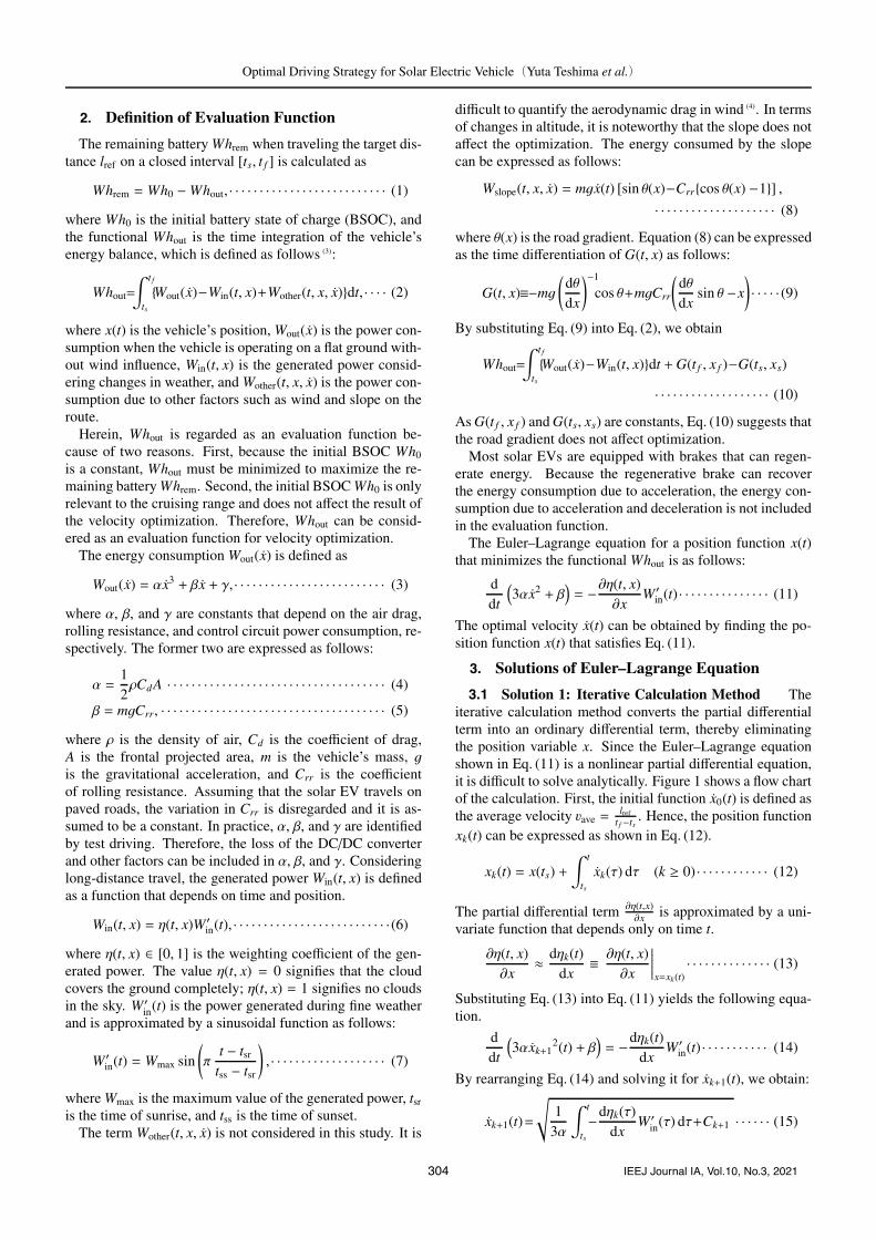
Fig. 2. A flow chart of an optimization example (n0 =15, nth = 150)

( 4 ) Return to step (1) until the stopping criterion (ni ≥nth) is satisfied.

Figure 2 shows a flow chart for when the initial division num-ber n0 is 15, and the threshold value nth is 150.4.1 Deciding Method of Search Radius Ci and Correc-

tion Vector ε In this method, the search radius Ci mustbe determined appropriately to reduce the computation timeand to find the correct solution. In this study, we define thesearch radius as follows:

Ci =t f − ts

ni−1· · · · · · · · · · · · · · · · · · · · · · · · · · · · · · · · · · · (26)

The correction vector ε functions as a weight factor fortCSi. The arrival time to the control stop Xi is assumed tomost likely change in the middle of the driving route. There-fore, the correction vector ε is defined such that it possessesweights in the middle of the route.

ε[ j]=

{k!

j!(k− j)!

}−d

(1 ≤ j ≤ k, 0 ≤ d ≤ 1), · · · · (27)

where d is the coefficient. When d is 0, no weight is implied;when d is 1, the weight is equal to the binominal distribution.

5. Simulation Results

5.1 Simulation Condition The simulation conditionsare presented in Table 1, and the specifications of the com-puter used in the simulations is shown in Table 2. The ve-hicle travels a distance of 450 km. The battery pack, whichcan store 13 kWh of energy, is fully charged at the start ofdriving. The simulation is based on Bridgestone World So-lar Challenge (BWSC), a solar-powered EV race that spansfrom Darwin to Adelaide (i.e., over 3022 km) in approxi-mately six days. The CSs in real applications include theloading/unloading and resting areas for the drivers. RecentBWSC regulations require smaller solar EVs and limitedpanel areas; hence, the performance assumed in this studycannot be achieved under the latest regulations. However, it

Table 1. Simulation conditionVehicle mass [kg] 1450

Maximum power [W] 4000

Coefficient of drag [-] 0.20

Frontal projected area [m2] 2.3

Rolling resistance [-] 0.006

Moving distance [km] 450

Battery capacity [kWh] 13

Transfer time [min] 360

Table 2. Specification of computer used in simulation

Processor AMD A10-7870K

RAM 16 GB

Operating System Windows 10 Home

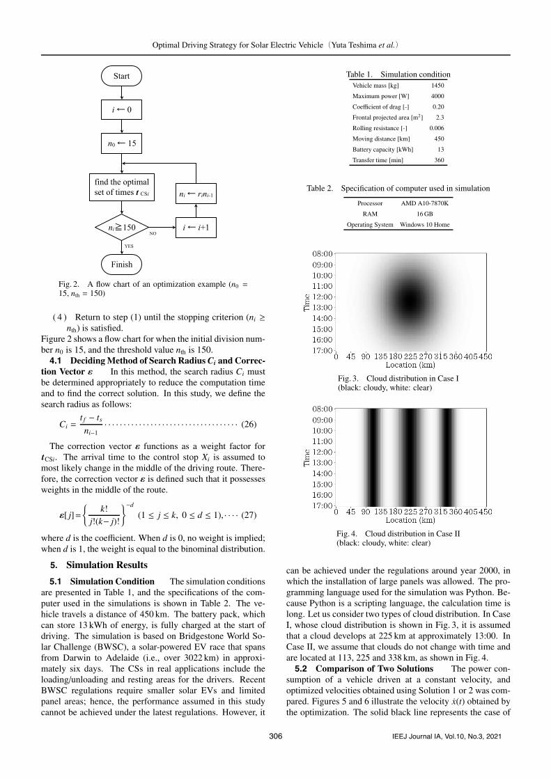
Fig. 3. Cloud distribution in Case I(black: cloudy, white: clear)

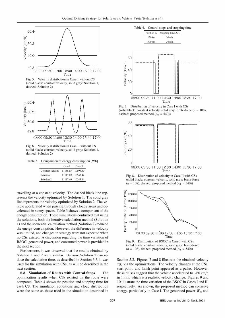
Fig. 4. Cloud distribution in Case II(black: cloudy, white: clear)

can be achieved under the regulations around year 2000, inwhich the installation of large panels was allowed. The pro-gramming language used for the simulation was Python. Be-cause Python is a scripting language, the calculation time islong. Let us consider two types of cloud distribution. In CaseI, whose cloud distribution is shown in Fig. 3, it is assumedthat a cloud develops at 225 km at approximately 13:00. InCase II, we assume that clouds do not change with time andare located at 113, 225 and 338 km, as shown in Fig. 4.5.2 Comparison of Two Solutions The power con-

sumption of a vehicle driven at a constant velocity, andoptimized velocities obtained using Solution 1 or 2 was com-pared. Figures 5 and 6 illustrate the velocity x(t) obtained bythe optimization. The solid black line represents the case of



Fig. 5. Velocity distribution in Case I without CS(solid black: constant velocity, solid gray: Solution 1,dashed: Solution 2)

Fig. 6. Velocity distribution in Case II without CS(solid black: constant velocity, solid gray: Solution 1,dashed: Solution 2)

Table 3. Comparison of energy consumption [Wh]

Case I Case II

Constant velocity 11158.55 10594.80

Solution 1 11117.69 10543.44

Solution 2 11117.69 10543.44

travelling at a constant velocity. The dashed black line rep-resents the velocity optimized by Solution 1. The solid grayline represents the velocity optimized by Solution 2. The ve-hicle accelerated when passing through cloudy areas and de-celerated in sunny spaces. Table 3 shows a comparison of theenergy consumption. These simulations confirmed that usingthe solutions, both the iterative calculation method (Solution1) and the sequential calculation method (Solution 2) reducedthe energy consumption. However, the difference in velocitywas limited, and changes in strategy were not expected whenno CSs existed. A discussion regarding the time variation ofBSOC, generated power, and consumed power is provided inthe next section.

Furthermore, it was observed that the results obtained bySolution 1 and 2 were similar. Because Solution 2 can re-duce the calculation time, as described in Section 3.3, it wasused for the simulation with CSs, as will be described in thenext section.5.3 Simulation of Routes with Control Stops The

optimization results when CSs existed on the route werecompared. Table 4 shows the position and stopping time foreach CS. The simulation conditions and cloud distributionwere the same as those used in the simulation described in

Table 4. Control stops and stopping time

Position xk Stopping time ΔTk

150 km 30 min

300 km 30 min

Fig. 7. Distribution of velocity in Case I with CSs(solid black: constant velocity, solid gray: brute-force (n = 108),dashed: proposed method (nth = 540))

Fig. 8. Distribution of velocity in Case II with CSs(solid black: constant velocity, solid gray: brute-force(n = 108), dashed: proposed method (nth = 540))

Fig. 9. Distribution of BSOC in Case I with CSs(solid black: constant velocity, solid gray: brute-force(n = 108), dashed: proposed method (nth = 540))

Section 5.2. Figures 7 and 8 illustrate the obtained velocityx(t) via the optimizations. The velocity changes at the CSs,start point, and finish point appeared as a pulse. However,these pulses suggest that the vehicle accelerated to ∼60 km/hin 1 min, which is a realistic velocity change. Figures 9 and10 illustrate the time variation of the BSOC in Cases I and II,respectively. As shown, the proposed method can conserveenergy, particularly in Case I. The generated power Win and



Fig. 10. Distribution of BSOC in Case II with CSs(solid black: constant velocity, solid gray: brute-force(n = 108), dashed: proposed method (nth = 540))

Fig. 11. Distribution of Win in Case I with CSs(solid black: constant velocity, solid gray: brute-force(n = 108), dashed: proposed method (nth = 540))

Fig. 12. Distribution of Win in Case II with CSs(solid black: constant velocity, solid gray: brute-force(n = 108), dashed: proposed method (nth = 540))

Fig. 13. Distribution of Wout in Case I with CSs(solid black: constant velocity, solid gray: brute-force(n = 108), dashed: proposed method (nth = 540))

Fig. 14. Distribution of Wout in Case II with CSs(solid black: constant velocity, solid gray: brute-force(n = 108), dashed: proposed method (nth = 540))

Fig. 15. Vehicle location and cloud distribution in Case I(solid black: route optimized by proposed method(nth = 540), dashed gray: constant velocity)

Fig. 16. Vehicle location and cloud distribution in Case II(solid black: route optimized by proposed method(nth = 540), dashed gray: constant velocity)

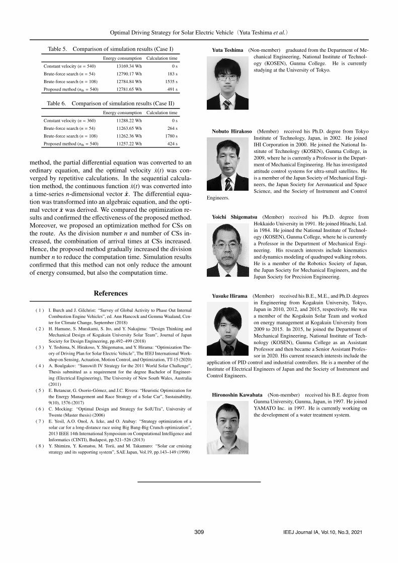
power consumption Wout in Case I are shown in Figs. 11 and13, respectively, and those of Case II are shown in Figs. 12and 14, respectively. Figures 15 and 16 show the routes trav-eled by the vehicle, where a gradual slope indicates a quickpassage. It is clear that in the optimized route, the vehiclequickly passed through the cloudy spots. The energy con-sumption improved owing to the optimization, as shown inTables 5 and 6. Moreover, the calculation time reduced sig-nificantly when the method proposed herein was used.

6. Conclusion

We defined the evaluation function Whout and derived theEuler–Lagrange equation. Two solutions were proposedherein for the equation: the iterative calculation method andthe sequential calculation method. In the iterative calculation



Table 5. Comparison of simulation results (Case I)

Energy consumption Calculation time

Constant velocity (n = 540) 13169.34 Wh 0 s

Brute-force search (n = 54) 12790.17 Wh 183 s


Proposed method (nth = 540) 12781.65 Wh 491 s

Table 6. Comparison of simulation results (Case II)

Energy consumption Calculation time

Constant velocity (n = 360) 11288.22 Wh 0 s



Proposed method (nth = 540) 11257.22 Wh 424 s

method, the partial differential equation was converted to anordinary equation, and the optimal velocity x(t) was con-verged by repetitive calculations. In the sequential calcula-tion method, the continuous function x(t) was converted intoa time-series n-dimensional vector x. The differential equa-tion was transformed into an algebraic equation, and the opti-mal vector x was derived. We compared the optimization re-sults and confirmed the effectiveness of the proposed method.Moreover, we proposed an optimization method for CSs onthe route. As the division number n and number of CSs in-creased, the combination of arrival times at CSs increased.Hence, the proposed method gradually increased the divisionnumber n to reduce the computation time. Simulation resultsconfirmed that this method can not only reduce the amountof energy consumed, but also the computation time.

References

( 1 ) I. Burch and J. Gilchrist: “Survey of Global Activity to Phase Out InternalCombustion Engine Vehicles”, ed. Ann Hancock and Gemma Waaland, Cen-ter for Climate Change, September (2018)

( 2 ) H. Hamane, S. Murakami, S. Ito, and Y. Nakajima: “Design Thinking andMechanical Design of Kogakuin University Solar Team”, Journal of JapanSociety for Design Engineering, pp.492–499 (2018)

( 3 ) Y. Teshima, N. Hirakoso, Y. Shigematsu, and Y. Hirama: “Optimization The-ory of Driving Plan for Solar Electric Vehicle”, The IEEJ International Work-shop on Sensing, Actuation, Motion Control, and Optimization, TT-15 (2020)

( 4 ) A. Boulgakov: “Sunswift IV Strategy for the 2011 World Solar Challenge”,Thesis submitted as a requirement for the degree Bachelor of Engineer-ing (Electrical Engineering), The University of New South Wales, Australia(2011)

( 5 ) E. Betancur, G. Osorio-Gomez, and J.C. Rivera: “Heuristic Optimization forthe Energy Management and Race Strategy of a Solar Car”, Sustainability,9(10), 1576 (2017)

( 6 ) C. Mocking: “Optimal Design and Strategy for SolUTra”, University ofTwente (Master thesis) (2006)

( 7 ) E. Yesil, A.O. Onol, A. Icke, and O. Atabay: “Strategy optimization of asolar car for a long-distance race using Big Bang-Big Crunch optimization”,2013 IEEE 14th International Symposium on Computational Intelligence andInformatics (CINTI), Budapest, pp.521–526 (2013)

( 8 ) Y. Shimizu, Y. Komatsu, M. Torii, and M. Takamuro: “Solar car cruisingstrategy and its supporting system”, SAE Japan, Vol.19, pp.143–149 (1998)

Yuta Teshima (Non-member) graduated from the Department of Me-chanical Engineering, National Institute of Technol-ogy (KOSEN), Gunma College. He is currentlystudying at the University of Tokyo.

Nobuto Hirakoso (Member) received his Ph.D. degree from TokyoInstitute of Technology, Japan, in 2002. He joinedIHI Corporation in 2000. He joined the National In-stitute of Technology (KOSEN), Gunma College, in2009, where he is currently a Professor in the Depart-ment of Mechanical Engineering. He has investigatedattitude control systems for ultra-small satellites. Heis a member of the Japan Society of Mechanical Engi-neers, the Japan Society for Aeronautical and SpaceScience, and the Society of Instrument and Control

Engineers.

Yoichi Shigematsu (Member) received his Ph.D. degree fromHokkaido University in 1991. He joined Hitachi, Ltd.in 1984. He joined the National Institute of Technol-ogy (KOSEN), Gunma College, where he is currentlya Professor in the Department of Mechanical Engi-neering. His research interests include kinematicsand dynamics modeling of quadruped walking robots.He is a member of the Robotics Society of Japan,the Japan Society for Mechanical Engineers, and theJapan Society for Precision Engineering.

Yusuke Hirama (Member) received his B.E., M.E., and Ph.D. degreesin Engineering from Kogakuin University, Tokyo,Japan in 2010, 2012, and 2015, respectively. He wasa member of the Kogakuin Solar Team and workedon energy management at Kogakuin University from2009 to 2015. In 2015, he joined the Department ofMechanical Engineering, National Institute of Tech-nology (KOSEN), Gunma College as an AssistantProfessor and then became a Senior Assistant Profes-sor in 2020. His current research interests include the

application of PID control and industrial controllers. He is a member of theInstitute of Electrical Engineers of Japan and the Society of Instrument andControl Engineers.

Hironoshin Kawabata (Non-member) received his B.E. degree fromGunma University, Gunma, Japan, in 1997. He joinedYAMATO Inc. in 1997. He is currently working onthe development of a water treatment system.


Documents

Optimal Driving Strategy for Solar Electric Vehicle