OPSM 301 Operations Management Class 22: Aggregate Planning (Chapter 13) Koç University Zeynep Aksin [email protected]

OPSM 301 Operations Management

Class 22:Aggregate Planning (Chapter 13)

Koç University

Zeynep [email protected]

Announcements

Reminder: Midterm 2 next Tuesday on 20/12 at 17:00 CAS-Z08

Aggregate Planning: will skip AP in services; however OPSM 405 Service Operations Management has an extensive module on this topic

Linear Programming: Quantitative Module B; will skip graphical solution and sensitivity analysis parts

Example 2: Finding Cu and Co

A textile company in UK orders coats from China. They buy a coat from 250€ and sell for 325€. If they cannot sell a coat in winter, they sell it at a discount price of 225€. When the demand is more than what they have in stock, they have an option of having emergency delivery of coats from Ireland, at a price of 290.

The demand for winter has a normal distribution with mean 32,500 and std dev 6750.

How much should they order from China??

Operations Planning

Order Scheduling

Material RequirementPlanning

Master ProductionScheduling

Daily workforce and customerscheduling

Weekly workforce andCustomer scheduling

Aggregate Planning

Strategic CapacityPlanning

Process Planning

Long

range

Medium range

Short

range

Manufacturing Service

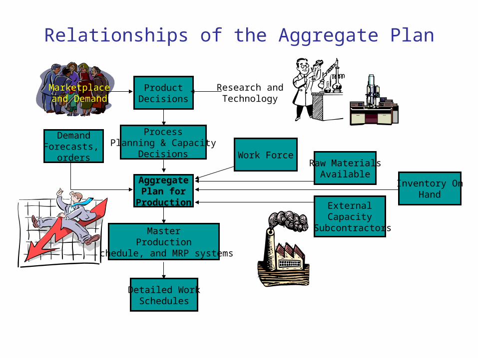
Relationships of the Aggregate Plan

AggregatePlan for

Production

DemandForecasts,

orders

MasterProduction

Schedule, and MRP systems

Detailed WorkSchedules

ExternalCapacity

Subcontractors

Inventory OnHand

Raw MaterialsAvailable

Work Force

Marketplaceand Demand

Research andTechnology

ProductDecisions

ProcessPlanning & Capacity

Decisions

Provides the quantity and timing of production for intermediate future– Usually 3 to 18 months into future

Combines (‘aggregates’) production– Often expressed in common units

• Example: Hours, dollars, equivalents (e.g., FTE students)

Involves capacity and demand variables

Aggregate Planning

Meet demand Use capacity efficiently Meet inventory policy Minimize cost

– Labor

– Inventory

– Plant & equipment

– Subcontract

Aggregate Planning Goals

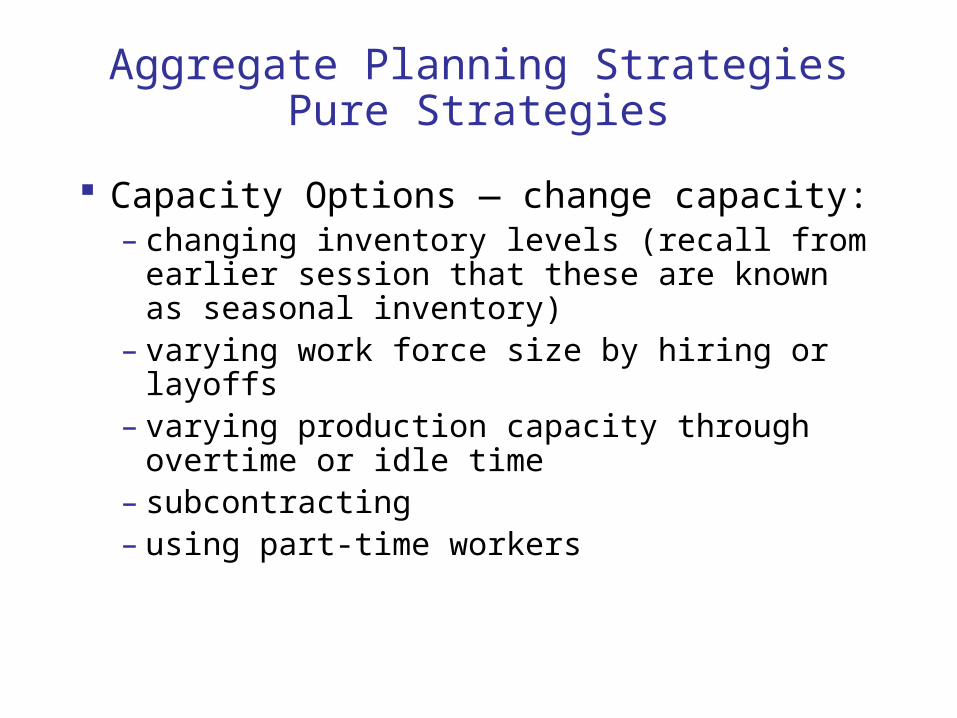
Aggregate Planning StrategiesPure Strategies

Capacity Options — change capacity:– changing inventory levels (recall from

earlier session that these are known as seasonal inventory)

– varying work force size by hiring or layoffs– varying production capacity through

overtime or idle time– subcontracting– using part-time workers

Aggregate Planning StrategiesPure Strategies

Demand Options — change demand:

– influencing demand– backordering during high demand periods– counterseasonal product mixing

Aggregate Scheduling Options - Advantages and Disadvantages

Option Advantage Disadvantage SomeComments

Changinginventory levels

Changes inhuman resourcesare gradual, notabruptproductionchanges

Inventoryholding costs;Shortages mayresult in lostsales

Applies mainlyto production,not service,operations

Varyingworkforce sizeby hiring orlayoffs

Avoids use ofother alternatives

Hiring, layoff,and trainingcosts

Used where sizeof labor pool islarge


Varyingproduction ratesthrough overtimeor idle time

Matches seasonalfluctuationswithouthiring/trainingcosts

Overtimepremiums, tiredworkers, may notmeet demand

Allowsflexibility withinthe aggregateplan

Subcontracting Permitsflexibility andsmoothing of thefirm's output

Loss of qualitycontrol; reducedprofits; loss offuture business

Applies mainlyin productionsettings

Advantages/Disadvantages - Continued

Advantages/Disadvantages - Continued


Using part-timeworkers

Less costly andmore flexiblethan full-timeworkers

Highturnover/trainingcosts; qualitysuffers;schedulingdifficult

Good forunskilled jobs inareas with largetemporary laborpools

Influencingdemand

Tries to useexcess capacity.Discounts drawnew customers.

Uncertainty indemand. Hard tomatch demand tosupply exactly.

Createsmarketing ideas.Overbookingused in somebusinesses.

Advantage/Disadvantage - Continued


Back orderingduring high-demand periods

May avoidovertime. Keepscapacity constant

Customer mustbe willing towait, butgoodwill is lost.

Many companiesbackorder.

Counterseasonalproducts andservice mixing

Fully utilizesresources; allowsstable workforce.

May requireskills orequipmentoutside a firm'sareas ofexpertise.

Risky findingproducts orservices withopposite demandpatterns.

The Extremes

Level Strategy

Chase Strategy

Production equals

demand

Production rate is constant

Example 1:M

onth

ly s

ales

for

ecas

ts (

$ m

illi

on)

Jan

Feb

Mar

Apr

May

Jun.

July

Aug

Sep

t.

Oct

.

Nov

.

Dec

.

7.6 8.4 10.2 9.0 11.8 7.0 8.6 12.6 14.4 12.8 15.8 11.8

Total sales for the year = $130 million

Cumulative ChartC

umul

ativ

e sa

les

fore

cast

s ($

mil

lion

)

Jan

Feb

Mar

Apr

May

Jun.

July

Aug

Sep

t.

Oct

.

Nov

.

Dec

.

120-

Chase Strategy

Cum

ulat

ive

sale

s fo

reca

sts

($ m

illi

on)

Jan

Feb

Mar

Apr

May

Jun.

July

Aug

Sep

t.

Oct

.

Nov

.

Dec

.

120-

Cumulative sales and

cumulative production

Level Strategy

Cum

ulat

ive

sale

s fo

reca

sts

($ m

illi

on)

Jan

Feb

Mar

Apr

May

Jun.

July

Aug

Sep

t.

Oct

.

Nov

.

Dec

.

120-

Cumulative sales

Cumulative production

shortage

excess

Labor Capacity Requirements

January 253 20 1581 28.4 3099February 280 21 1667 29.6 5933March 340 23 1848 33.1 8037April 300 20 1875 33.7 9737May 393 22 2235 40.2 9706…. … … ….. …. ….December 393 20 2458 44.2 0Total 4333 243 2229 40 7035

Sales i

n

labor

-hou

rs

(000

)s Wor

king

days

Variab

le wor

k

force Vari

able

work

week Vari

able

inven

tory

Chase Strategy Level Strategy

Illustration of calculations

Level production– Total sales = $130 million– Total labor-hours required = $130 million/$30 = 4.333 M

labor-hrs.– Total hours = 243 days . 8 hrs/day = 1944 hrs– Number of workers = 4.333 M / 1944 = 2229

Variable workforce for January– Sales in labor-hours = $7.6 M /$30 = 253,333– Working hours = 20 days . 8 hrs/day = 160 hours– Variable work force = 1581

Variable workweek for January– Sales in labor-hours = $7.6 M /$30 = 253,333– Number of workers = 2229 (average required, constant)– Variable monthly load for a worker = 253,333/2229 = 113.65– Variable workweek = 113.65/4 = 28.4 hours/week

Variable inventory for January (Level production)– Production in January =

(2229 workers)(20 days/month)(8 hrs/day) = 356,640– Demand for January = 253,333 (labor-hours)– Inventory = 103,307 labor-hours– Inventory ($) = (103,307)($30/labor-hour) = $309,920

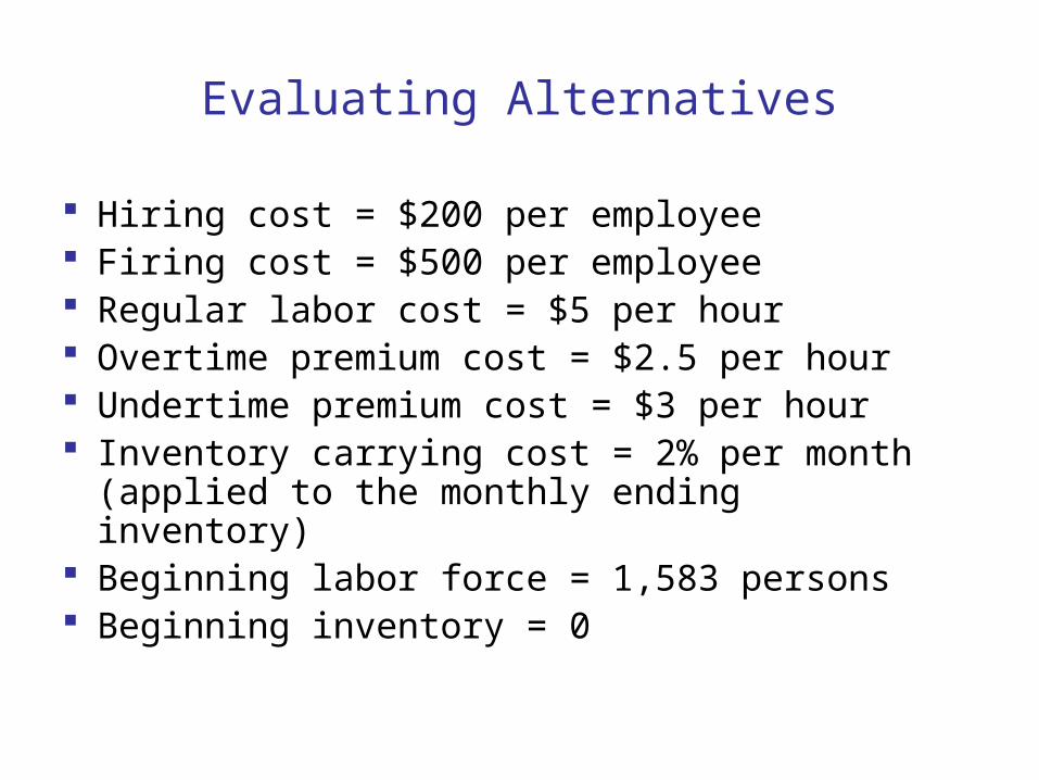
Evaluating Alternatives

Hiring cost = $200 per employee Firing cost = $500 per employee Regular labor cost = $5 per hour Overtime premium cost = $2.5 per hour Undertime premium cost = $3 per hour Inventory carrying cost = 2% per month

(applied to the monthly ending inventory) Beginning labor force = 1,583 persons Beginning inventory = 0

Alternative 1: Variable Workforce

Zero-inventory, hire-fire as requiredStarting Required Hire-fire CostWorkforce Workforce

January 1,583 1,583 0 0February 1,583 1,667 84 $16,800 March 1,667 1,848 181 $36,200April 1,848 1,875 27 $5,400May 1,875 2,235 360 $72,000June 2,235 1,326 -909 $454,500 …. ….. ……. ……. ……...December3,292 2,458 -834 $417,000Total $2,708,300

Alternative 2: Level Production

constant worforce :2229, Variable Inventory

Initial hire = (2229-1583) = 646 Cost = 129,200

Initial Production Required Ending Cost Inventory (labor-hours) Inventory

January 0 356,640 253,333 103,307 $61984.2…. ….. ……. ……. ……...

Total $1,882,420

Example 2:

National Steel Corporation (NSC) produces a special-purpose steel used in the aircraft and aerospace industries. The Sales Department of NSC has received orders of 2400, 2200, 2700, and 2500 tons of steel for each of the next 4 months. NSC can meet these demands by producing the steel, by drawing from its inventory, or by using any combination of the two alternatives.

The production costs per ton of steel during each of the next 4 months are projected to be $7400, $7500, $7600, and $7650. Because costs are rising each month-due to inflationary pressures- NSC might be better off producing more steel than it needs in a given month and storing the excess.

Production capacity cannot exceed 4000 tons in any one month. The monthly production is finished at the end of the month, at which time the demand is met. Any remaining steel is then stored in inventory at a cost of $120 per ton for each month it remains there.

If the production level is increased from one month to the next, then the company incurs a cost of $50 per ton of increased production to cover the additional labor and/or overtime. Each ton of decreased production to cover the additional labor and/or overtime. Each ton of decreased production incurs a cost of $30 to cover the benefits of unused employees.

The production level during the previous month was 1800 tons, and the beginning inventory is 1000 tons. Inventory at the end of the fourth month must be at least 1500 tons to cover anticipated demand.Formulate a production plan for NSC that minimizes the total costs over the next 4 months.

Data for the Production-Planning Problem of NSC

Month 1 2 3 4

Demand (tons) 2400 2200 2700 2500Production cost ($/ton) 7400 7500 7600 7650Inventory cost ($/ton/month) 120 120 120 120 Starting inventory = 1000 tonsEnding inventory (at the end of 4th month) = 1500 tonsStarting production level = 1800 tonsCost of changing production level = $50 per ton (increase)

$30 per ton (decrease)

Documents

OPSM 301 Operations Management Class 22: Aggregate Planning (Chapter 13) Koç University Zeynep Aksin [email protected]