Embed Size (px)
Citation preview
OPSM 501: Operations Management
Week 5:
Batching
EOQ
Koç University Graduate School of BusinessMBA Program
Zeynep [email protected]
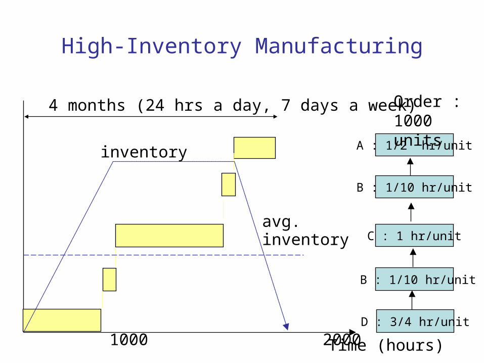
High-Inventory Manufacturing
D : 3/4 hr/unit
B : 1/10 hr/unit
C : 1 hr/unit
B : 1/10 hr/unit
A : 1/2 hr/unit
Time (hours) 1000 2000
4 months (24 hrs a day, 7 days a week)
inventory
avg.inventory
Order :1000 units
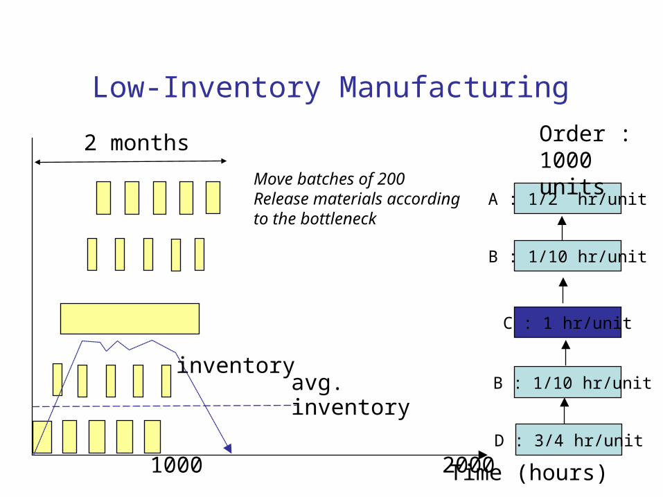
Low-Inventory Manufacturing
D : 3/4 hr/unit
B : 1/10 hr/unit
C : 1 hr/unit
B : 1/10 hr/unit
A : 1/2 hr/unit
Time (hours) 1000 2000
2 months
avg.inventory
Order :1000 units
inventory
Move batches of 200Release materials according to the bottleneck

When do you detect quality problems?
D
B
C
B
A
Damage done
Quality control
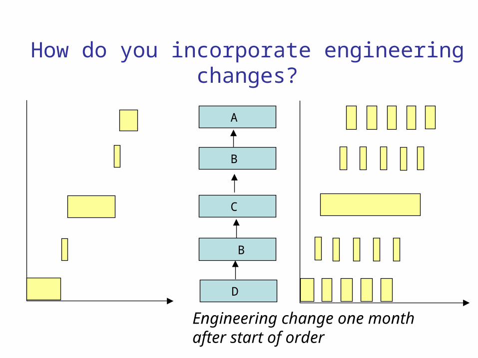
How do you incorporate engineering changes?
D
B
C
B
A
Engineering change one month after start of order
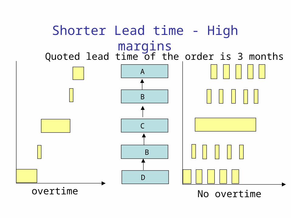
Shorter Lead time - High margins
D
B
C
B
A
overtime No overtime
Quoted lead time of the order is 3 months

Due-date performance
D
B
C
B
A
Forecast validity
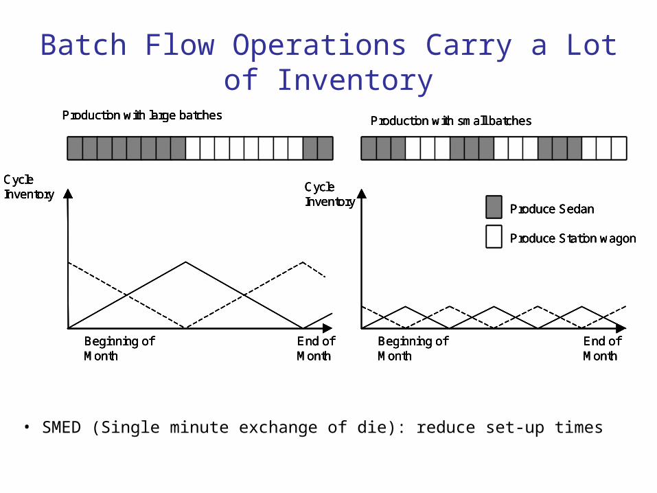
Production with large batches Production with small batches
CycleInventory
End ofMonth
Beginning ofMonth
CycleInventory
End ofMonth
Beginning ofMonth
Produce Sedan
Produce Station wagon
Production with large batches Production with small batches
CycleInventory
End ofMonth
Beginning ofMonth
CycleInventory
End ofMonth
Beginning ofMonth
Produce Sedan
Produce Station wagon
Production with large batches Production with small batches
CycleInventory
End ofMonth
Beginning ofMonth
CycleInventory
End ofMonth
Beginning ofMonth
Produce Sedan
Produce Station wagon
Production with large batches Production with small batches
CycleInventory
End ofMonth
Beginning ofMonth
CycleInventory
End ofMonth
Beginning ofMonth
Produce Sedan
Produce Station wagon
• SMED (Single minute exchange of die): reduce set-up times
Batch Flow Operations Carry a Lot of Inventory
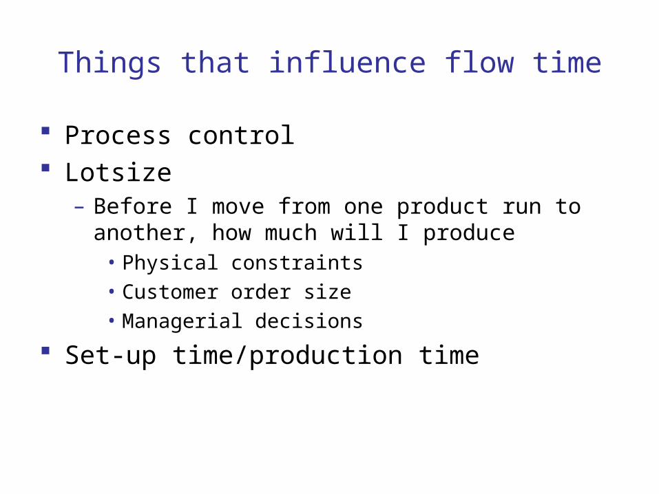
Things that influence flow time
Process control Lotsize
– Before I move from one product run to another, how much will I produce
• Physical constraints
• Customer order size
• Managerial decisions
Set-up time/production time
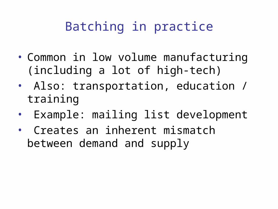
Batching in practice
• Common in low volume manufacturing (including a lot of high-tech)
• Also: transportation, education / training• Example: mailing list development• Creates an inherent mismatch between demand
and supply
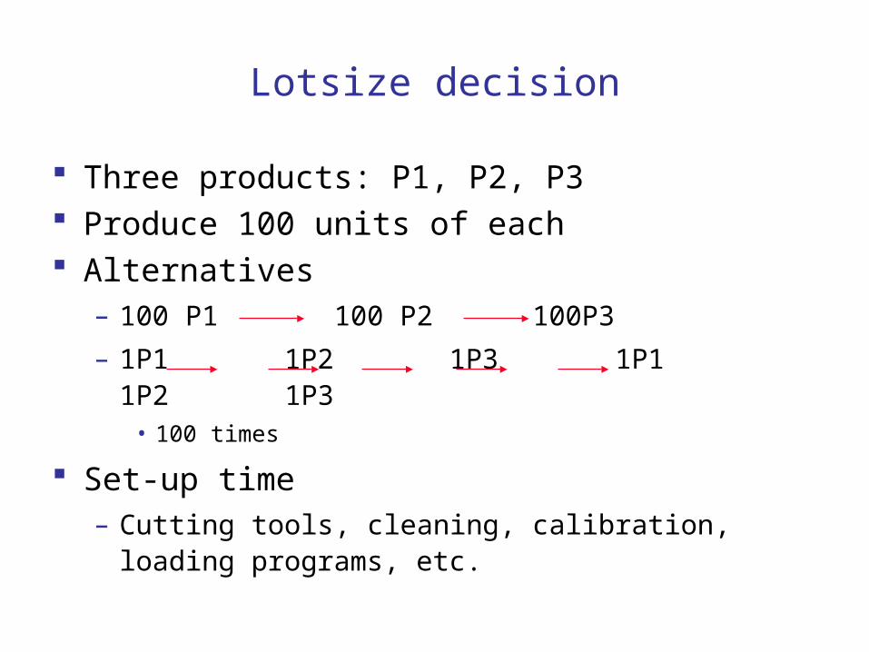
Lotsize decision
Three products: P1, P2, P3 Produce 100 units of each Alternatives
– 100 P1 100 P2 100P3
– 1P1 1P2 1P3 1P1 1P2 1P3• 100 times
Set-up time– Cutting tools, cleaning, calibration, loading programs, etc.
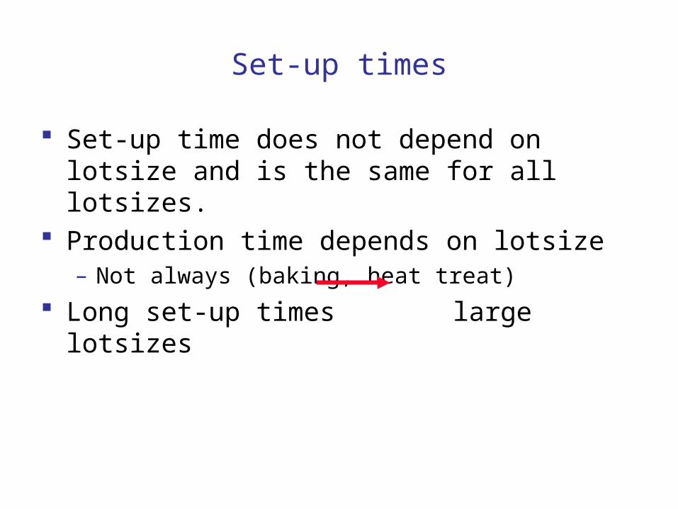
Set-up times
Set-up time does not depend on lotsize and is the same for all lotsizes.
Production time depends on lotsize– Not always (baking, heat treat)
Long set-up times large lotsizes

Example
P1,P2,P3 example– Set-up time 60 min.– Production time 10 min/unit– Need 3 of each type
Try the alternatives– 1P1, 1P2, 1P3, 1P1, 1P2, 1P3, 1P1, 1P2, 1P3
– 3P1, 3P2, 3P3
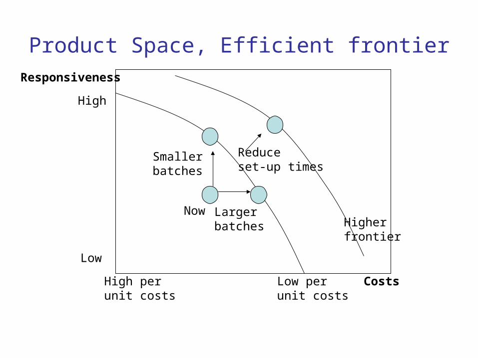
Responsiveness
Costs
High
Low
High perunit costs
Low perunit costs
Now
Smaller batches
Largerbatches
Reduce set-up times
Higherfrontier
Product Space, Efficient frontier
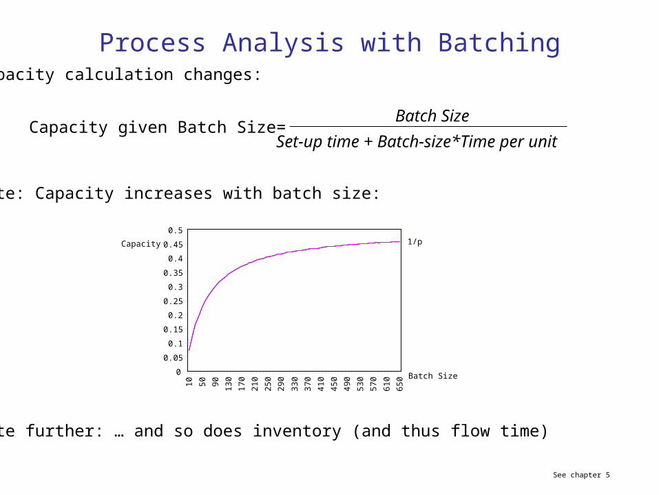
• Capacity calculation changes:
• Note: Capacity increases with batch size:
• Note further: … and so does inventory (and thus flow time)
Batch Size
Set-up time + Batch-size*Time per unitCapacity given Batch Size=
Capacity 1/p
0
0.05
0.1
0.15
0.2
0.25
0.3
0.35
0.4
0.45
0.5
10
50
90
13
0
17
0
21
0
25
0
29
0
33
0
37
0
41
0
45
0
49
0
53
0
57
0
61
0
65
0 Batch Size
See chapter 5
Process Analysis with Batching
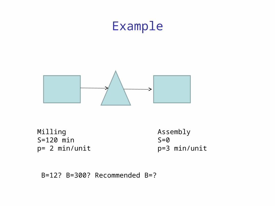
Example
MillingS=120 minp= 2 min/unit
AssemblyS=0p=3 min/unit
B=12? B=300? Recommended B=?
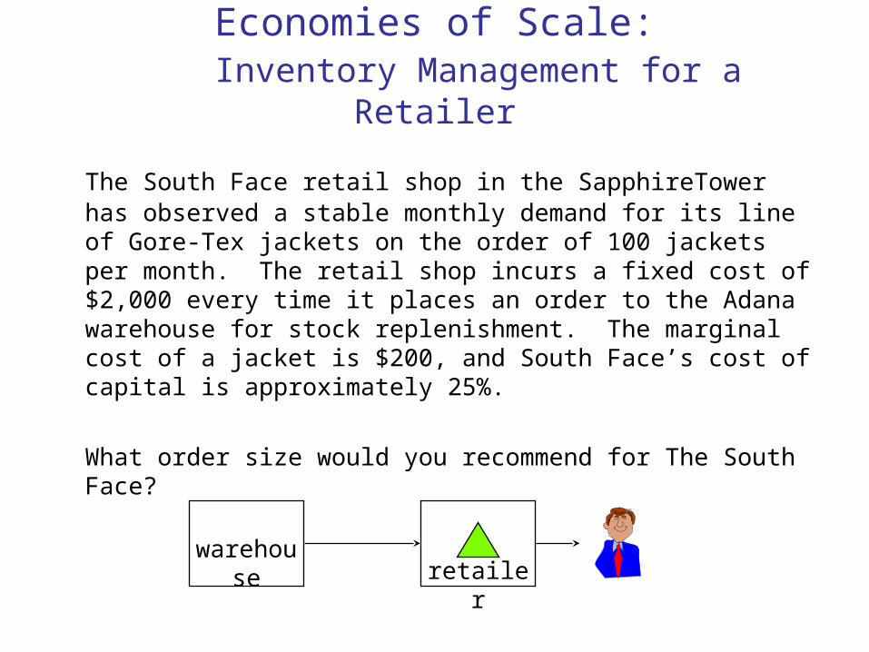
Economies of Scale:Inventory Management for a Retailer
The South Face retail shop in the SapphireTower has observed a stable monthly demand for its line of Gore-Tex jackets on the order of 100 jackets per month. The retail shop incurs a fixed cost of $2,000 every time it places an order to the Adana warehouse for stock replenishment. The marginal cost of a jacket is $200, and South Face’s cost of capital is approximately 25%.
What order size would you recommend for The South Face?
retailerwarehouse
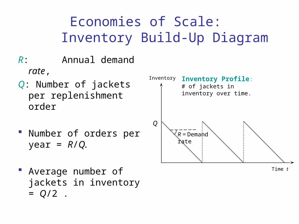
Economies of Scale: Inventory Build-Up Diagram
R: Annual demand rate,
Q: Number of jackets per replenishment order
Number of orders per year = R/Q.
Average number of jackets in inventory = Q/2 .
Q
Time t
Inventory Profile:# of jackets in inventory over time.
R = Demand rate
Inventory
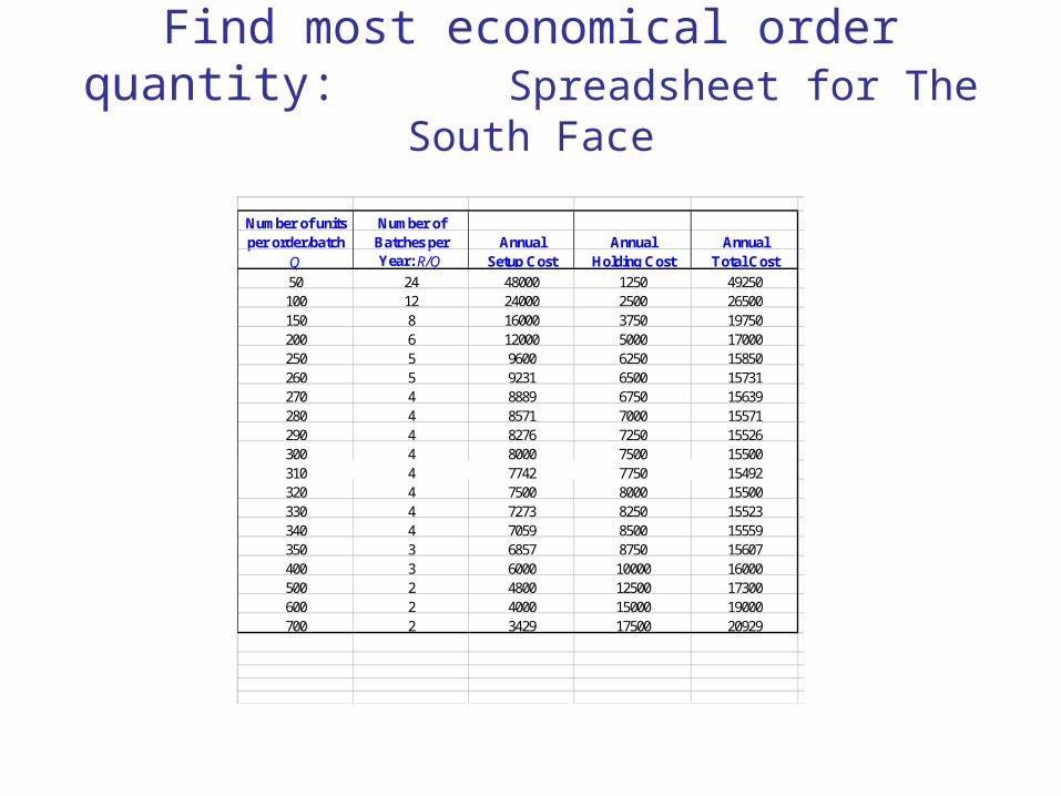
Find most economical order quantity: Spreadsheet for The South Face
Number of units Number ofper order/batch Batches per Annual Annual Annual
Q Year: R/Q Setup Cost Holding Cost Total Cost
50 24 48000 1250 49250100 12 24000 2500 26500150 8 16000 3750 19750200 6 12000 5000 17000250 5 9600 6250 15850260 5 9231 6500 15731270 4 8889 6750 15639280 4 8571 7000 15571290 4 8276 7250 15526300 4 8000 7500 15500310 4 7742 7750 15492320 4 7500 8000 15500330 4 7273 8250 15523340 4 7059 8500 15559350 3 6857 8750 15607400 3 6000 10000 16000500 2 4800 12500 17300600 2 4000 15000 19000700 2 3429 17500 20929
H2
Q S +
Q
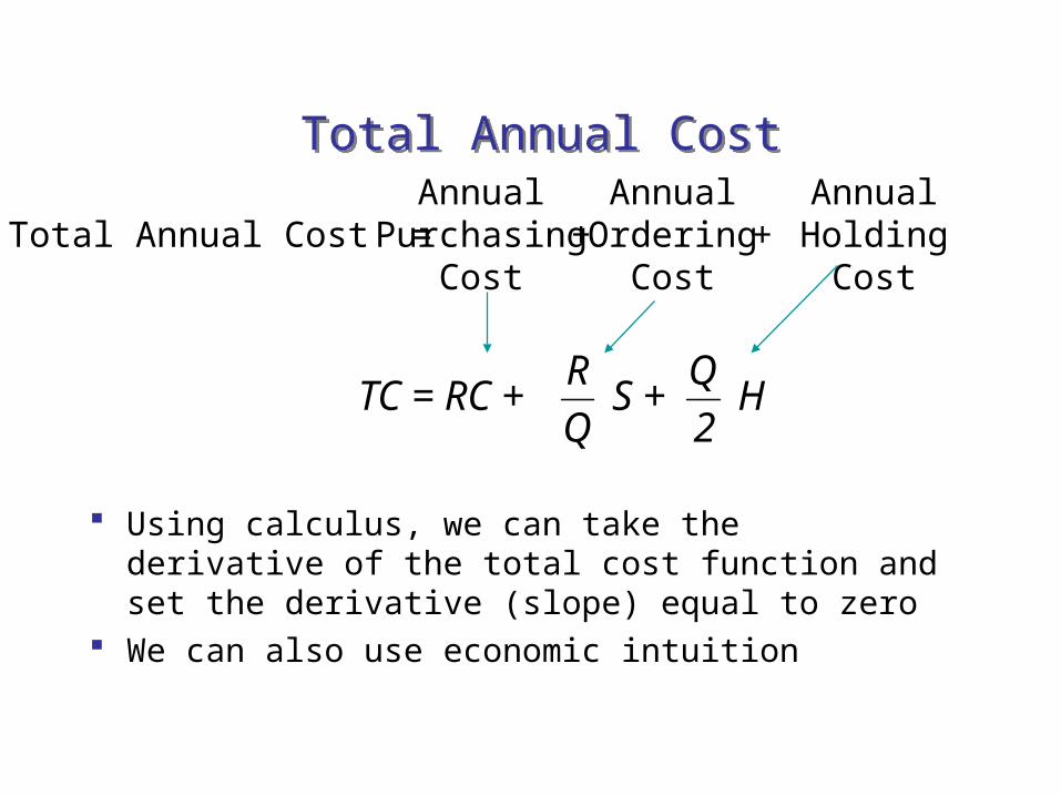
RTC = RC +
Total Annual CostTotal Annual Cost
Total Annual Cost = Annual
PurchasingCost
AnnualOrdering
Cost
AnnualHolding
Cost+ +
Using calculus, we can take the derivative of the total cost function and set the derivative (slope) equal to zero
We can also use economic intuition
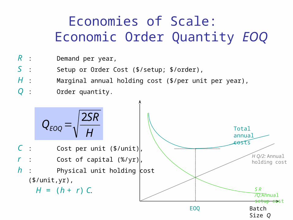
Economies of Scale: Economic Order Quantity EOQ
R : Demand per year,
S : Setup or Order Cost ($/setup; $/order),
H : Marginal annual holding cost ($/per unit per year),
Q : Order quantity.
C : Cost per unit ($/unit),
r : Cost of capital (%/yr),
h : Physical unit holding cost
($/unit,yr),
H = (h + r) C.
H
SRQEOQ
2
Batch Size Q
Total annual costs
H Q/2: Annual holding cost
S R /Q:Annual setup cost
EOQ
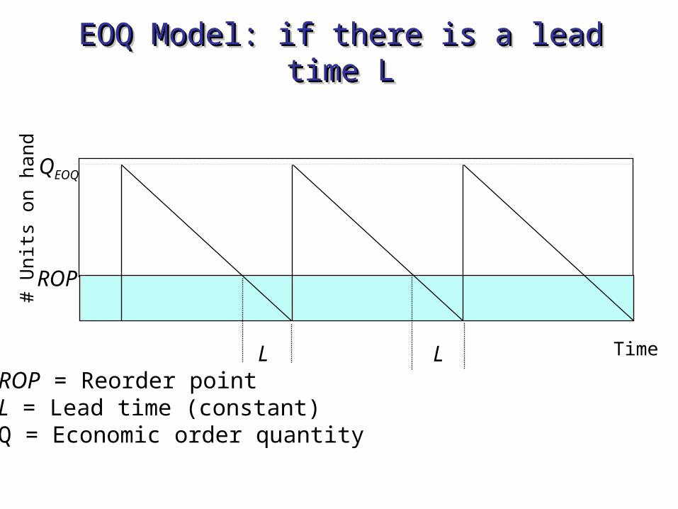
EOQ Model: if there is a lead time LEOQ Model: if there is a lead time LEOQ Model: if there is a lead time LEOQ Model: if there is a lead time L
ROP = Reorder point L = Lead time (constant)Q = Economic order quantity
L L
ROP
Time
# U
nit
s on
han
dQEOQ
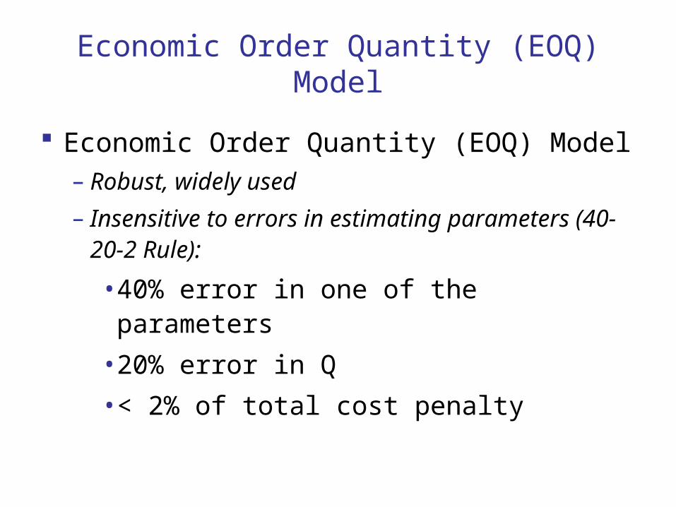
Economic Order Quantity (EOQ) Model
Economic Order Quantity (EOQ) Model– Robust, widely used
– Insensitive to errors in estimating parameters (40-20-2 Rule):
• 40% error in one of the parameters
• 20% error in Q
•< 2% of total cost penalty
Learning Objectives: Batching & Economies of Scale
Increasing batch size of production (or purchase) increases average inventories (and thus cycle times).
Average inventory for a batch size of Q is Q/2. The optimal batch size trades off setup cost and holding cost. To reduce batch size, one has to reduce setup cost (time). Square-root relationship between Q and (R, S):
– If demand increases by a factor of 4, it is optimal to increase batch size by a factor of 2 and produce (order) twice as often.
– To reduce batch size by a factor of 2, setup cost has to be reduced by a factor of 4.
Announcements
HW 2 is due next time The Goal is due next time Have a nice break!