Embed Size (px)
Citation preview
OperationsResearch:
An Introduction
Eighth Edition
Hamdy A. TahaUniversity of Arkansas, Fayetteville
Upper Saddle River, New Jersey 07458
Library of Congress Calaloging.in-Publicalion Data
Taha, Hamdy A.Operations research: an introduction I Hamdy A. Taha.~8th ed.
p. ern.Includes bibliographical references and index_ISBN 0-13-188923·01. Operations research. 2. Programming (Mathematics) 1. Title.
T57.6.T3 199796-37160003 -dc21
96-37160
Vice President and Editorial Director, ECS: Marcia J. HortonSenior Editor: Holly StarkExecutive Managing Editor: Vince O'BrienManaging Editor: David A. GeorgeProduction Editor: Craig LittleDirector of Creative Services: Paul BelfantiArt Director: Jayne ConteCover Designer: Bruce KenselaarArt Editor: Greg DullesManufacturing Manager: Alexis HeydJ-LongManufacturing Buyer: Lisa McDowell
_
_ © 2007 by Pearson Education, Inc.Pearson Prentice Hall
• - . Pearson Education, Inc.. Upper Saddle River, NJ 07458
All rights reserved. No part of this book may be reproduced, in any form or by any means, without permission in writing from the publisher.
Pearson Prentice Hall"" is a trademark of Pearson Education, Inc.
Preliminary edition, first, and second editions © 1968,1971 and 1976, respectively, by Hamdy A. Taha.Third, fourth, and fifth editions © 1982,1987, and 1992, respectively, by Macmillan Publishing Company.Sixth and seventh editions © 1997 and 2003, respectively, by Pearson Education, Inc.
The author and publisher of this book have used their best efforts in preparing this book. These effortsinclude the development, research, and testing of the theories and programs to determine their effectiveness. The author and publisher make no warranty of any kind, expressed or implied, with regard to theseprograms or the documentation contained in this book. The author and publisher shall not be liable in anyevent for incidental or consequential damages in connection with, or arising out of, the furnishing, performance, or use of these programs.
Printed in the United States of America10 9 8 7 6 5 4 3 2
ISBN 0-13-188923-0Pearson Education Ltd., LondonPearson Education Australia Pty. Ltd., SydneyPearson Education Singapore, Pte. Ltd.Pearson Education North Asia Ltd., Hong KongPearson Education Canada, Inc., TorontoPearson Educaci6n de Mexico, S.A. de C. V.Pearson Education-Japan, TokyoPearson Education Malaysia, Pte. Ltd.Pearson Education, Inc., Upper Saddle River, New Jersey
To Karen
Los rios no llevan agua,el sallas fuentes sec6 ...
jYo se donde hay una fuenteque no ha de secar el sol!La fuente que no se agotaes mi propio coraz6n ...
-li: RuizAguilera (1862)

Contents
Preface xvii
About the Author xix
Trademarks xx
Chapter 1
Chapter 2
Chapter 3
What Is Operations Research? 1
1.1 Operations Research Models 11.2 Solving the OR Model 41.3 Queuing and Simulation Mode!s 51.4 Art of Modeling 51.5 More Than Just Mathematics 71.6 Phases of an OR Study 81.7 About This Book 10
References 10
Modeling with Linear Programming 11
2.1 Two-Variable LP Model 122.2 Graphical LP Solution 15
2.2.1 Solution of a Maximization Model 162.2.2 Solution of a Minimization Model 23
12.3 Selected LP Applications 272.3.1 Urban Planning 272.3.2 Currency Arbitrage 322.3.3 Investment 372.3.4 Production Planning and Inventory Control 422.3.5 Blending and Refining 512.3.6 Manpower Planning 572.3.7 Additional Applications 60
2.4 Computer Solution with Excel Solver and AMPL 682.4.1 lP Solution with Excel Solver 692.4.2 LP Solution with AMPl 73References 80
The Simplex Method and Sensitivity Analysis 81
3.1 LP Model in Equation Form 823.1.1 Converting Inequalities into Equations
with Nonnegative Right-Hand Side 823.1.2 Dealing with Unrestricted Variables '84
3.2 Transition from Graphical to Algebraic Solution 85
vii
viii Contents
Chapter 4
Chapter 5
3.3 The Simplex Method 903.3.1 Iterative Nature of the Simplex Method 903.3.2 Computational Details of the Simplex Algorithm 933.3.3 Summary of the Simplex Method 99
3.4 Artificial Starting Solution 1033.4.1 M-Method 1043.4.2 Two-Phase Method 108
3.5 Special Cases in the Simplex Method 1133.5.1 Degeneracy 1133.5.2 Alternative Optima 1163.5.3 Unbounded Solution 1193.5.4 Infeasible Solution 121
3.6 Sensitivity Analysis 1233.6.1 Graphical Sensitivity Analysis 1233.6.2 Algebraic Sensitivity Analysis-Changes in the Right-
Hand Side 1293.6.3 Algebraic Sensitivity Analysis-Objective Function 1393.6.4 Sensitivity Analysis with TORA, Solver, and AMPL 146References 150
Duality and Post-Optimal Analysis 151
4.1 Definition of the Dual Problem 1514.2 Primal-Dual Relationships 156
4.2.1 Review of Simple Matrix Operations 1564.2.2 Simplex Tableau Layout 1584.2.3 Optimal Dual Solution 1594.2.4 Simplex Tableau Computations 165
4.3 Economic Interpretation of Duality 1694.3.1 Economic Interpretation of Dual Variables 1704.3.2 Economic Interpretation of Dual Constraints 172
4.4 Additional Simplex Algorithms 1744.4.1 Dual Simplex Method 1744.4.2 Generalized Simplex Algorithm 180
4.5 Post-Optimal Analysis 1814.5.1 Changes Affecting Feasibility 1824.5.2 Changes Affecting Optimality 187References 191
Transportation Model and Its Variants 193
5.1 Definition of the Transportation Model 1945.2 Nontraditional Transportation Models 2015.3 The Transportation Algorithm 206
5.3.1 Determination of the Starting Solution 2075.3.2 Iterative Computations of the Transportation
Algorithm 211
Chapter 6
Chapter 7
Contents ix
5.3.3 Simplex Method Explanation of the Methodof Multipliers 220
5.4 The Assignment Model 2215.4.1 The Hungarian Method 2225.4.2 Simplex Explanation of the Hungarian Method 228
5.5 The Transshipment Model 229References 234
Network Models 235
6.1 Scope and Definition of Network Models 2366.2 Minimal Spanning Tree Algorithm 2396.3 Shortest-Route Problem 243
6.3.1 Examples of the Shortest-Route Applications 2436.3.2 Shortest-Route Algorithms 2486.3.3 Linear Programming Formulation
of the Shortest-Route Problem 2576.4 Maximal flow model 263
6.4.1 Enumeration of Cuts 2636.4.2 Maximal-Flow Algorithm 2646.4.3 Linear Programming Formulation of Maximal
Flow Mode 2736.5 (PM and PERT 275
6.5.1 Network Representation 2776.5.2 Critical Path (CPM) Computations 2826.5.3 Construction of the Time Schedule 2856.5.4 Linear Programming Formulation of CPM 2926.5.5 PERT Calculations 293References 296
Advanced Linear Programming 297
7.1 Simplex Method Fundamentals 2987.1.1 From Extreme Points to Basic Solutions 3007.1.2 Generalized Simplex Tableau in Matrix Form 303
7.2 Revised Simplex Method 3067.2.1 Development of the Optimality and Feasibility
Conditions 3077.2.2 Revised Simplex Algorithm 309
7.3 Bounded-Variables Algorithm 3157.4 Duality 321
7.4.1 Matrix Definition of the Dual Problem 3221.4.2 Optimal Dual Solution 322
7.5 Parametric Linear Programming 3267.5.1 Parametric Changes in ( 3277.5.2 Parametric Changes in b 330References 332
x Contents
Chapter 8 Goal Programming 333
8.1 A Goal Programming Formulation 3348.2 Goal Programming Algorithms 338
8.2.1 The Weights Method 3388.2.2 The Preemptive Method 341References 348
Chapter 9 Integer Linear Programming 349
9.1 Illustrative Applications 3509.1.1 Capital Budgeting 3509.1.2 Set-Covering Problem 3549.1.3 Fixed-Charge Problem 3609.1.4 Either-Or and If-Then Constraints 364
9.2 Integer Programming Algorithms 3699.2.1 Branch-and-Bound (B&B) Algorithm 3709.2.2 Cutting-Plane Algorithm 3799.2.3 Computational Considerations in IlP 384
9.3 Traveling Salesperson Problem (TSP) 3859.3.1 Heuristic Algorithms 3899.3.2 B&B Solution Algorithm 3929.3.3 Cutting-Plane Algorithm 395References 397
Chapter 10 Deterministic Dynamic Programming 399
10.1 Recursive Nature of Computations in DP 40010.2 Forward and Backward Recursion 40310.3 Selected DP Applications 405
10.3.1 KnapsackJFly-Away/Cargo-loading Model 40510.3.2 Work-Force Size Model 41310.3.3 Equipment Replacement Model 41610.3.4 Investment Model 42010.3.5 Inventory Models 423
10.4 Problem of Dimensionality 424References 426
Chapter 11 Deterministic Inventory Models 427
11.1 General Inventory Model 42711.2 Role of Demand in the Development of Inventory
Models 42811.3 Static Ecol1omic-Order-Quantity (EOQ) Models 430
11.3.1 Classic EOQ model 43011.3.2 EOQ with Price Breaks 43611.3.3 Multi-Item EOQ with Storage Limitation 440
11.4 Dynamic EOQ Models 44311.4.1 No-Setup Model 44511.4.2 Setup Model 449References 461
Contents xi
Chapter 12 Review of Basic: Probability 463
12.1 laws of Probability 46312.1.1 Addition Law of Probability 46412.1.2 Conditional Law of Probability 465
12.2 Random Variables and Probability Distributions 46712.3 Expectation of a Random Variable 469
12.3.1 Mean and Variance (Standard Deviation) of a RandomVariable 470
12.3.2 Mean and Variance of Joint Random Variables 47212.4 Four Common Probability Distributions 475
12.4.1 Binomial Distribution 47512.4.2 Poisson Distribution 47612.4.3 Negative Exponential Distribution 47712.4.4 Normal Distribution 478
12.5 Empirical Distributions 481References 488
Chapter 13 Decision Analysis and Games 489
13.1 Decision Making under Certainty-Analytic HierarchyProcess (AHP) 490
13.2 Decision Making under Risk 50013.2.1 Decision Tree-Based Expected Value Criterion 50013.2.2 Variations of the Expected Value Criterion 506
13.3 Decision under Uncertainty 51513.4 Game Theory 520
13.4.1 Optimal Solution of Two-Person Zero-Sum Games 52113.4.2 Solution of Mixed Strategy Games 524References 530
Chapter 14 Probabilistic: Inventory Models 531
14.1 Continuous Review Models 53214.1.1 "Probabilitized" EOQ Model 53214.1.2 Probabilistic EOQ Model 534
14.2 Single-Period Models 53914.2.1 No-Setup Model (Newsvendor Model) 53914.2.2 Setup Model (5-5 Policy) 543
14.3 Multiperiod Model 545References 548
Chapter 15 Queuing Systems 549
15.1 Why Study Queues? 55015.2 Elements of a Queuing Model 55115.3 Role of Exponential Distribution 55315.4 Pure Birth and Death Models (Relationship Between
the Exponential and Poisson Distributions) 55615.4.1 Pure Birth Model 55615.4.2 Pure Death Model 560
xii Table of Contents
15.5 Generalized Poisson Queuing Model 56315.6 Specialized Poisson Queues 568
15.6.1 Steady-State Measures of Performance 569. 15.6.2 Single-Server Models 573
15.6.3 Multiple-Server Models 58215.6.4 Machine Servicing Model-{MIMIR): (GDIKIK).
R> K 59215.7 (M/G/1 ):(GDI 00 100 )-Pollaczek-Khintchine (P-K)
Formula 59515.8 Other Queuing Models 59715.9 Queuing Decision Models 597
15.9.1 Cost Models 59815.9.2 Aspiration Level Model 602References 604
Chapter 16 Simulation Modeling 605
16.1 Monte Carlo Simulation 60516.2 Types of Simulation 61016.3 Elements of Discrete-Event Simulation 611
16.3.1 Generic Definition of Events 61116.3.2 Sampling from Probability Distributions 613
16.4 Generation of Random Numbers 62216.5 Mechanics of Discrete Simulation 624
16.5.1 Manual Simulation of a Single-Server Model 62416.5.2 Spreadsheet-Based Simulation of the Single-Server
Model 63016.6 Methods for Gathering Statistical Observations 633
16.6.1 Subinterval Method 63416.6.2 Replication Method 63516.6.3 Regenerative (Cycle) Method 636
16.7 Simulation Languages 638References 640
Chapter 17 Markov Chains 641
17.1 Definition of a Markov Chain 64117.2 Absolute and n-Step Transition Probabilities 64417.3 Classification of the States in a Markov Chain 64617.4 Steady-State Probabilities and Mean Return Times
of Ergodic Chains 64917.5 First Passage Time 65417.6 Analysis of Absorbing States 658
References 663
Chapter 18 Classical Optimization Theory. 665
18.1 Unconstrained Problems 66518.1.1 Necessary and Sufficient Conditions 67618.1.2 The Newton-Raphson Method 670
Table of Contents xiii
18.2 Constrained Problems 67218.2.1 Equality Constraints 67318.2.2 Inequality Constraints-Karush-Kuhn-Tucker
(KKT) Conditions 685References 690
Chapter 19 Nonlinear Programming Algorithms 691
19.1 Unconstrained Algorithms 69119.1.1 Direct Search Method 69119.1.2 Gradient Method 695
19.2 Constrained Algorithms 69919.2.1 Separable Programming 69919.2.2 Quadratic Programming 70819.2.3 Chance-Constrained Programming 71319.2.4 linear Combinations Method 71819.2.5 SUMT Algorithm 721References 722
Appendix A AMPL Modeling Language 723
A.1 A Rudimentary AMPl Model 723A.2 Components of AMPl Model 724A.3 Mathematical Expressions and Computed Parameters 732A.4 Subsets and Indexed Sets 735A.S Accessing External Files 737
A.S.1 Simple Read Files 737A.5.2 Using Print and Printf to Retrieve Output 739A.S.3 Input Table Files 739A.5.4 Output Table Files 742A.5.S Spreadsheet Input/Output Tables 744
A.6 Interactive Commands 744A.7 Iterative and Conditional Execution
of AMPl Commands 746A.8 Sensitivity Analysis Using AMPL 748
References 748
Appendix B Statistical Tables 749
Appendix C Partial Solutions to Seleded Problems 753
Index 803

h.
On the CD-ROM
Chapter 20 Additional Network and LP Algorithms CD-1
20.1 Minimum-Cost Capacitated Flow Problem CD-120.1.1 Network Representation CD-220.1.2 Linear Programming Formulation CD-420.1.3 Capacitated Network Simplex Algorithm CD-9
20.2 Decomposition Algorithm CD-1620.3 Karmarkar Interior-Point Method CD-25
20.3.1 Basic Idea of the Interior-Point Algorithm CD-2520.3.2 Interior-Point Algorithm CD-27References CD-36
Chapter 21 Forecasting Models CD-37
21.1 Moving Average Technique CD-3721.2 Exponential Smoothing CD-4121.3 Regression CD-42
References CD-46
Chapter 22 Probabilistic Dynamic Programming CD-47
22.1 A Game of Chance CD-4722.2 Investment Problem CD-5022.3 Maximization of the Event of Achieving a Goal CD-54
References CD-57
Chapter 23 Markovian Decision Process CD-58
23.1 Scope of the Markovian Decision Problem CD-5823.2 Finite-Stage Dynamic Programming Model CD-6023.3 Infinite-Stage Model CD-64
23.3.1 Exhaustive Enumeration Method CD-5423.3.2 Policy Iteration Method Without Discounting CD-5723.3.3 Policy Iteration Method with Discounting CD-70
23.4 linear Programming Solution CD-73References CD-77
Chapter 24 Case Analysis CD·79
Case 1: Airline Fuel Allocation Using Optimum Tankering CD-79Case 2: Optimization of Heart Valves ProductionCD-86Case 3: Scheduling Appointments at Australian Tourist
Commission Trade Events CD-89
xv
jII,IiI
~ :xvi On the CD-ROM
Case 4: Saving Federal Travel Dollars CD-93Case 5: Optimal Ship Routing and Personnel Assignments
for Naval Recruitment in Thailand CD-97Case 6: Allocation of Operating Room Time in Mount Sinai
Hospital CD-103Case 7: Optimizing Trailer Payloads at PFG Building Glass 107Case 8: Optimization of Crosscutting and Log Allocation at
VVeyerhauser 113Case 9: Layout Planning for a Computer Integrated Manufacturing
(CIM) Facility CD-118Case 10: Booking Limits in Hotel Reservations CD-125Case 11: Casey's Problem: Interpreting and Evaluating a
New Test CD-128Case 12: Ordering Golfers on the Final Day of Ryder Cup
Matches CD-131Case 13: Inventory Decisions in Dell's Supply Chain CD-133Case 14: Analysis of Internal Transport System in a
Manufacturing Plant CD-136Case 15: Telephone Sales Manpower Planning at Qantas
Airways CD-139
Appendix D Review of Vectors and Matrices CD-145
0.1 Vectors CD-1450.1.1 Definition of a Vector CD-1450.1.2 Addition (Subtraction) of Vectors CD-1450.1.3 Multiplication of Vectors by Scalars CO-1460.1.4 linearly Independent Vectors CD-146
0.2 Matrices CD-1460.2.1 Definition of a Matrix CO-1460.2.2 Types of Matrices CO-1460.2.3 Matrix Arithmetic Operations CD-147D.2.4 Determinant of a Square Matrix CO-1480.2.5 Nonsingular Matrix CO-1500.2.6 Inverse of a Nonsingular Matrix CD-ISO0.2.7 Methods of Computing the Inverse of Matrix CO-151D.2.8 Matrix Manipulations with Excel CO-156
0.3 Quadratic Forms CD-1570.4 Convex and Concave Functions CD-159Problems 159Selected References 160
Appendix E case Studies CD·161
Preface
The eighth edition is a major revision that streamlines the presentation of the text material with emphasis on the applications and computations in operations research:
• Chapter 2 is dedicated to linear programming modeling, with applications in theareas of urban renewal, currency arbitrage, investment, production planning,blending, scheduling, and trim loss. New end-of-section problems deal with topicsranging from water quality management and traffic control to warfare.
• Chapter 3 presents the general LP sensitivity analysis, including dual prices andreduced costs, in a simple and straightforward manner as a direct extension of thesimplex tableau computations.
• Chapter 4 is now dedicated to LP post-optimal analysis based on duality.• An Excel-based combined nearest neighbor-reversal heuristic is presented for
the traveling salesperson problem.• Markov chains treatment has been expanded into new Chapter 17.• The totally new Chapter 24* presents 15 fully developed real-life applications.
The analysis, which often cuts across more than one OR technique (e.g., heuristicsand LP, or ILP and queuing), deals with the modeling, data collection, and computational aspects of solving the problem. These applications are cross-referencedin pertinent chapters to provide an appreciation of the use of OR techniques inpractice.
• The new Appendix E* includes approximately 50 mini cases of real-life situationscategorized by chapters.
• More than 1000 end-of-section problem are included in the book.• Each chapter starts with a study guide that facilitates the understanding of the
material and the effective use of the accompanying software.• The integration of software in the text allows testing concepts that otherwise
could not be presented effectively:1. Excel spreadsheet implementations are used throughout the book, includ
ing dynamic programming, traveling salesperson, inventory, AHP, Bayes'probabilities, "electronic" statistical tables, queuing, simulation, Markovchains, and nonlinear programming. The interactive user input in somespreadsheets promotes a better understanding of the underlying techniques.
2. The use of Excel Solver has been expanded throughout the book, particularly in the areas of linear, network, integer, and nonlinear programming.
3. The powerful commercial modeling language, AMPL®, has been integratedin the book using numerous examples ranging from linear and network to
'Contained on the CD-ROM.
xvii
xviii Preface
integer and nonlinear programming. The syntax of AMPL is given in AppendixA and its material cross-referenced within the examples in the book.
4. TORA continue to play the key role of tutorial software.• All computer-related material has been deliberately compartmentalized either in
separate sections or as subsection titled AMPL/Excel/Solver/TORA moment tominimize disruptions in the main presentation in the book.
To keep the page count at a manageable level, some sections, complete chapters,and two appendixes have been moved to the accompanying CD. The selection of the.excised material is based on the author's judgment regarding frequency of use in introductory OR classes.
ACKNOWLEDGMENTS
I wish to acknowledge the importance of the seventh edition reviews provided byLayek L. Abdel-Malek, New Jersey Institute of Technology, Evangelos Triantaphyllou,Louisiana State University, Michael Branson, Oklahoma State University, Charles H.Reilly, University of Central Florida, and Mazen Arafeh, Virginia Polytechnic Instituteand State University. In particular, lowe special thanks to two individuals who have influenced my thinking during the preparation of the eighth edition: R. Michael Harnett(Kansas State University), who over the years has provided me with valuable feedbackregarding the organization and the contents of the book, and Richard H. Bernhard(North Carolina State University), whose detailed critique of the seventh editionprompted a reorganization of the opening chapters in this edition.
Robert Fourer (Northwestern University) patiently provided me with valuablefeedback about the AMPL material presented in this edition. I appreciate his help inediting the material and for suggesting changes that made the presentation more readable. I also wish to acknowledge his help in securing permissions to include the AMPLstudent version and the solvers CPLEX, KNITRO, LPSOLVE, LOQO, and MINOS onthe accompanying CD.
As always, I remain indebted to my colleagues and to hundreds of students for theircomments and their encouragement. In particular, I wish to acknowledge the support I receive from Yuh-Wen Chen (Da-Yeh University, Taiwan), Miguel Crispin (University ofTexas, El Paso), David Elizandro (Tennessee Tech University), Rafael Gutierrez (University of Texas, El Paso), Yasser Hosni (University of Central Florida), Erhan Kutanoglu(University of Texas, Austin), Robert E. Lewis (United States Army Management Engineering College), Gino Lim (University of Houston), Scott Mason (University ofArkansas), Heather Nachtman (University of Arkanas), Manuel Rossetti (University ofArkansas), Tarek Taha (JB Hunt, Inc.), and Nabeel Yousef (University of Central Florida).
I wish to express my sincere appreciation to the Pearson Prentice Hall editorialand production teams for their superb assistance during the production of the book:Dee Bernhard (Associate Editor), David George (Production Manager - Engineering),Bob Lentz (Copy Editor), Craig Little (Production Editor), and Holly Stark (SeniorAcquisitions Editor).
HAMDY A. TAHA
[email protected]://ineg.uark.edurrahaORbook/

About the Author
Hamdy A. Taha is a University ProfessorEmeritus of Industrial Engineering with theUniversity of Arkansas, where he taught andconducted research in operations researchand simulation. He is the author of threeother books on integer programming andsimulation, and his works have been translatedinto Malay, Chinese, Korean, Spanish, Japanese,Russian, Turkish, and Indonesian. He is alsothe author of several book chapters, and histechnical articles have appeared in EuropeanJournal of Operations Research, IEEETransactions on Reliability, IlE Transactions,Interfaces, Management Science, Naval ResearchLogistics QuarterLy, Operations Research, andSimulation.Professor Taha was the recipient of the
Alumni Award for excellence in research and the university-wide Nadine BaumAward for excellence in teaching, both from the University of Arkansas, and numerousother research and teaching awards from the College of Engineering, University ofArkansas. He was also named a Senior Fulbright Scholar to Carlos III University,Madrid, Spain. He is fluent in three languages and has held teaching and consultingpositions in Europe, Mexico, and the Middle East.
xix
xx
Trademarks
AMPL is a registered trademark of AMPL Optimization, LLC, 900 Sierra PI. SE,Albuquerque, NM 87108-3379.
CPLEX is a registered trademark of ILOG, Inc., 1080 Linda Vista Ave., MountainView, CA 94043. .
KNITRO is a registered trademark of Ziena Optimization Inc., 1801 Maple Ave,Evanston, IL 6020l.
LOQO is a trademark of Princeton University, Princeton, NJ 08544.Microsoft, Windows, and Excel registered trademarks of Microsoft Corporation in the
United States and/or other countries.MINOS is a trademark of Stanford University, Stanford, CA 94305.Solver is a trademark of Frontline Systems, Inc., 7617 Little River Turnpike, Suite 960,
Annandale, VA 22003.TORA is a trademark of SimTec, Inc., PO. Box 3492, Fayetteville,AR 72702
Note: Other product and company names that are mentioned herein may be trademarks or registered trademarks of their respective owners in the United States and/orother countries.
t .. __
1.1
CHAPTER 1
What Is Operations Research?
Chapter Guide. The first formal activities of Operations Research (OR) were initiatedin England during World War II, when a team of British scientists set out to make scientifically based decisions regarding the best utilization of war materiel. After the war,the ideas advanced in military operations were adapted to improve efficiency and productivity in the civilian sector.
This chapter will familiarize you with the basic terminology of operations research, including mathematical modeling, feasible solutions, optimization, and iterativecomputations. You will learn that defining the problem correctly is the most important(and most difficult) phase of practicing OR. The chapter also emphasizes that, whilemathematical modeling is a cornerstone of OR, intangible (unquantifiable) factors(such as human behavior) must be accounted for in the final decision. As you proceedthrough the book, you will be presented with a variety of applications through solvedexamples and chapter problems. In particular, Chapter 24 (on the CD) is entirely devoted to the presentation of fully developed case analyses. Chapter materials are crossreferenced with the cases to provide an appreciation of the use of OR in practice.
1.1 OPERATIONS RESEARCH MODELS
Imagine that you have a 5-week business commitment between Fayetteville (FYV)and Denver (DEN). You fly out of Fayetteville on Mondays and return on Wednesdays. A regular round-trip ticket costs $400, but a 20% discount is granted if the datesof the ticket span a weekend. A one-way ticket in either direction costs 75% of the regular price. How should you buy the tickets for the 5-week period?
We can look at the situation as a decision-making problem whose solution requires answering three questions:
1. What are the decision alternatives?2. Under what restrictions is the decision made?
3. What is an appropriate objective criterion for evaluating the alternati-ves?
1
2 Chapter 1 What Is Operations Research?
Three alternatives are considered:
1. Buy five regular FYV-DEN-FYV for departure on Monday and return on Wednesday of the same week.
2. Buy one FYV-DEN, four DEN-FYV-DEN that span weekends, and one DENFYV.
3. Buy one FYV-DEN-FYV to cover Monday of the first week and Wednesday ofthe last week and four DEN-FYV-DEN to cover the remaining legs. All tickets inthis alternative span at least one weekend.
The restriction on these options is that you should be able to leave FYV on Mondayand return on Wednesday of the same week.
An obvious objective criterion for evaluating the proposed alternative is theprice of the tickets. The alternative that yields the smallest cost is the best. Specifically,we have
Alternative 1 cost = 5 X 400 = $2000
Alternative 2 cost = .75 X 400 + 4 X (.8 X 400) + .75 X 400 = $1880
Alternative 3 cost = 5 X (.8 X 400) = $1600
Thus, you should choose alternative 3.Though the preceding example illustrates the three main components of an OR
model-alternatives, objective criterion, and constraints-situations differ in the details of how each component is developed and constructed. To illustrate this point, consider forming a maximum-area rectangle out of a piece of wire of length L inches. Whatshould be the width and height of the rectangle?
In contrast with the tickets example, the number of alternatives in the present example is not finite; namely, the width and height of the rectangle can assume an infinitenumber of values. To formalize this observation, the alternatives of the problem areidentified by defining the width and height as continuous (algebraic) variables.
Let
w = width of the rectangle in inches
h = height of the rectangle in inches
Based on these definitions, the restrictions of the situation can be expressed verbally as
1. Width of rectangle + Height of rectangle = Half the length of the wire2. Width and height cannot be negative
These restrictions are translated algebraically as
1. 2(w + h) = L2. w ~ 0, h ;?: 0
1.1 Operations Research Models 3
The only remaining component now is the objective of the problem; namely,maximization of the area of the rectangle. Let z be the area of the rectangle, then thecomplete model becomes
Maximize z = wh
subject to
2(w + h) = L
w, h 2:: 0
The optimal solution of this model is w = h = ~, which calls for constructing a squareshape.
Based on the preceding two examples, the general OR model can be organized inthe following general format:
Maximize or minimize Objective Function
subject to
Constraints
A solution of the mode is feasible if it satisfies all the constraints. It is optimal if,in addition to being feasible, it yields the best (maximum or minimum) value of the objective function. In the tickets example, the problem presents three feasible alternatives, with the third alternative yielding the optimal solution. In the rectangle problem,a feasible alternative must satisfy the condition w + h = ~ with wand h assumingnonnegative values. This leads to an infinite number of feasible solutions and, unlikethe tickets problem, the optimum solution is determined by an appropriate mathematical tool (in this case, differential calculus).
Though OR models are designed to "optimize" a specific objective criterion subject to a set of constraints, the quality of the resulting solution depends on the completeness of the model in representing the real system. Take, for example, the ticketsmodel. If one is not able to identify all the dominant alternatives for purchasing the tickets, then the resulting solution is optimum only relative to the choices represented in themodel. To be specific, if alternative 3 is left out of the model, then the resulting "optimum" solution would call for purchasing the tickets for $1880, which is a suboptimal solution. The conclusion is that "the" optimum solution of a model is best only for thatmodel. If the model happens to represent the real system reasonably well, then its solution is optimum also for the real situation.
PROBLEM SET 1.1A
L In the tickets example, identify a fourth feasible alternative.
2. In the rectangle problem, identify two feasible solutions and determine which one is better.
3. Determine the optimal solution of the rectangle problem. (Hint: Use the constraint to express the objective function in terms of one variable, then use differential c<iICufus.)
4 Chapter 1 What Is Operations Research?
4. Amy, Jim, John, and Kelly are standing on the east bank of a river and wish to croSs tothe west side using a canoe. The canoe can hold at most two people at a time. Amy, beingthe most athletic, can row across the river in 1 minute. Jim, John, and Kelly would take 2,5, and 10 minutes, respectively. If two people are in the canoe, the slower person dictatesthe crossing time. The objective is for all four people to be on the other side of the riverin the shortest time possible.
(a) Identify at least two feasible plans for crossing the river (remember, the canoe is theonly mode of transportation and it cannot be shuttled empty).
(b) Define the criterion for evaluating the alternatives.
*(C)1 What is the smallest time for moving all four people to the other side of the river?
*5. In a baseball game, Jim is the pitcher and Joe is the batter. Suppose that Jim can throweither a fast or a curve ball at random. If Joe correctly predicts a curve ball, he can maintain a .500 batting average, else if Jim throws a curve ball and Joe prepares for a fast ball,his batting average is kept down to .200. On the other hand, if Joe correctly predicts a fastball, he gets a .300 batting average, else his batting average is only .100.
(a) Define the alternatives for this situation.
(b) Define the objective function for the problem and discuss how it differs from thefamiliar optimization (maximization or minimization) of a criterion.
6. During the construction of a house, six joists of 24 feet each must be trimmed to the correct length of 23 feet. The operations for cutting a joist involve the following sequence:
1.~
Operation
1. Place joist on saw horses2. Measure correct length (23 feet)3. Mark cutting line for circular saw4. Trim joist to correct length5. Stack trimmed joist in a designated area
Time (seconds)
1555
2020
1.2
Three persons are involved: Two loaders must work simultaneously on operations 1,2,and 5, and one cutter handles operations 3 and 4. There are two pairs of saw horses onwhich untrimmed joists are placed in preparation for cutting, and each pair can hold upto three side-by-side joists. Suggest a good schedule for trimming the six joists.
SOLVING THE OR MODEL
In OR, we do not have a single general technique to solve all mathematical models thatcan arise in practice. Instead, the type and complexity of the mathematical model dictate the nature of the solution method. For example, in Section 1.1 the solution of thetickets problem requires simple ranking of alternatives based on the total purchasingprice, whereas the solution of the rectangle problem utilizes differential calculus to determine the maximum area.
The most prominent OR technique is linear programming. It is designed formodels with linear objective and constraint functions. Other techniques include integerprogramming (in which the variables assume integer values), dynamic programming
IAn asterisk (*) designates problems whose solution is provided in Appendix C.
1.4
~.
1.4 Art of Modeling 5
(in which the original model can be decomposed into more manageable subproblems),network programming (in which the problem can be modeled as a network), andnonlinear programming (in which functions of the model are nonlinear). These areonly a few among many available OR tools.
A peculiarity of most OR techniques is that solutions are not generally obtainedin (formulalike) closed forms. Instead, they are determined by algorithms. An algorithm provides fixed computational rules that are applied repetitively to the problem,with each repetition (called iteration) moving the solution closer to the optimum. Because the computations associated with each iteration are typically tedious and voluminous, it is imperative that these algorithms be executed on the computer.
Some mathematical models may be so complex that it is impossible to solve themby any of the available optimization algorithms. In such cases, it may be necessary toabandon the search for the optimal solution and simply seek a good solution usingheuristics or rules ofthumb.
1.3 QUEUING AND SIMULATION MODELS
Queuing and simulation deal with the study of waiting lines. They are not optimizationtechniques; rather, they determine measures of performance of the waiting lines, suchas average waiting time in queue, average waiting time for service, and utilization ofservice facilities.
Queuing models utilize probability and stochastic models to analyze waiting lines,and simulation estimates the measures of performance by imitating the behavior of thereal system. In a way, simulation may be regarded as the next best thing to observing areal system. The main difference between queuing and simulation is that queuing models are purely mathematical, and hence are subject to specific assumptions that limittheir scope of application. Simulation, on the other hand, is flexible and can be used toanalyze practically any queuing situation.
The use of simulation is not without drawbacks. TIle process of developing simulation models is costly in both time and resources. Moreover, the execution of simulation models, even on the fastest computer, is usually slow.
1.4 ART OF MODELING
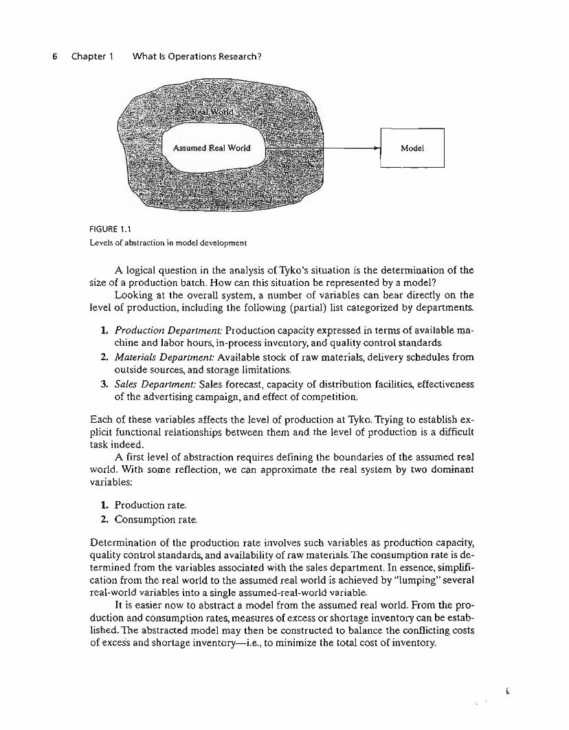
The illustrative models developed in Section 1.1 are true representations of real situations. This is a rare occurrence in OR, as the majority of applications usually involve(varying degrees of) approximations. Figure 1.1 depicts the levels of abstraction thatcharacterize the development of an OR model. We abstract the assumed real world.from the real situation by concentrating on the dominant variables that control the behavior of the real system. The model expresses in an amenable manner the mathematical functions that represent the behavior of the assumed real world.
To illustrate levels of abstraction in modeling, consider the Tyko ManufacturingCompany, where a variety of plastic containers are produced. When a production orderis issued to the production department, necessary raw materiars are acquired from thecompany's stocks or purchased from outside sources. Once the production batch iscompleted, the sales department takes charge of distributing the product to customers.
6 Chapter 1 What Is Operations Research?
Model
FIGURE 1.1
Levels of abstraction in model development
A logical question in the analysis of Tyko's situation is the determination of thesize of a production batch. How can this situation be represented by a model?
Looking at the overall system, a number of variables can bear directly on thelevel of production, including the following (partial) list categorized by departments.
1. Production Department: Production capacity expressed in terms of available machine and labor hours, in-process inventory, and quality control standards.
2. Materials Department: Available stock of raw materials, delivery schedules fromoutside sources, and storage limitations.
3. Sales Department: Sales forecast, capacity of distribution facilities, effectivenessof the advertising campaign, and effect of competition.
Each of these variables affects the level of production at Tyko. Trying to establish explicit functional relationships between them and the level of production is a difficulttask indeed.
A first level of abstraction requires defining the boundaries of the assumed realworld. With some reflection, we can approximate the real system by two dominantvariables:
1. Production rate.2. Consumption rate.
Determination of the production rate involves such variables as production capacity,quality control standards, and availability of raw materials. The consumption rate is determined from the variables associated with the sales department. In essence, simplification from the real world to the assumed real world is achieved by "lumping" severalreal-world variables into a single assumed-real-world variable.
It is easier now to abstract a model from the assumed real world. From the production and consumption rates, measures of excess or shortage inventory can be established. The abstracted model may then be constructed to balance the conflicting costsof excess and shortage inventory-i.e., to minimize the total cost of inventory.
1.5 More Than Just Mathematics 7
1.5 MORE THAN JUST MATHEMATICS
Because of the mathematical nature of OR models, one tends to think that an ORstudy is always rooted in mathematical analysis. Though mathematical modeling is acornerstone of OR, simpler approaches should be explored first. In some cases, a "common sense" solution may be reached through simple observations. Indeed, since thehuman element invariably affects most decision problems, a study of the psychology ofpeople may be key to solving the problem. Three illustrations are presented here tosupport this argument.
1. Responding to complaints of slow elevator service in a large office building,the OR team initially perceived the situation as a waiting-line problem that might require the use of mathematical queuing analysis or simulation. After studying the behavior of the people voicing the complaint, the psychologist on the team suggestedinstalling full-length mirrors at the entrance to the elevators. Miraculously the complaints disappeared, as people were kept occupied watching themselves and otherswhile waiting for the elevator.
2. In a study of the check-in facilities at a large British airport, a United StatesCanadian consulting team used queuing theory to investigate and analyze the situation. Part of the solution recommended the use of well-placed signs to urge passengerswho were within 20 minutes from departure time to advance to the head of the queueand request immediate service. The solution was not successful, because the passengers, being mostly British, were "conditioned to very strict queuing behavior" andhence were reluctant to move ahead of others waiting in the queue.
3. In a steel mill, ingots were first produced from iron ore and then used in themanufacture of steel bars and beams. The manager noticed a long delay between theingots production and their transfer to the next manufacturing phase (where end products were manufactured). Ideally, to reduce the reheating cost, manufacturing shouldstart soon after the ingots left the furnaces. Initially the problem was perceived as aline-balancing situation, which could be resolved either by reducing the output of ingots or by increasing the capacity of the manufacturing process. TIle OR team usedsimple charts to summarize the output of the furnaces during the three shifts of theday. They discovered that, even though the third shift started at 11:00 PM., most of theingots were produced between 2:00 and 7:00 A.M. Further investigation revealed thatthird-shift operators preferred to get long periods of rest at the start of the shift andthen make up for lost production during morning hours. The problem was solved by"leveling out" the production of ingots throughout the shift.
Three conclusions can be drawn from these illustrations:
1. Before embarking on sophisticated mathematical modeling, the OR teamshould explore the possibility of using "aggressive" ideas to resolve the situation. Thesolution of the elevator problem by installing mirrors is rooted in human psychologyrather than in mathematical modeling. It is also simpler and less costly than any recommendation a mathematical model might have produced. Perhaps this. is the reasonOR teams usually include the expertise of "outsiders" from nonmathernatical fields
III;
8 Chapter 1 What Is Operations Research?
(psychology in the case of the elevator problem). This point was recognized and implemented by the first OR team in Britain during World War II.
2. Solutions are rooted in people and not in technology. Any solution that doesnot take human behavior into account is apt to fail. Even though the mathematical solution of the British airport problem may have been sound, the fact that the consultingteam was not aware of the cultural differences between the United States and Britain(Americans and Canadians tend to be less formal) resulted in an unimplementablerecommendation.
3. An OR study should never start with a bias toward using a specific mathematical tool before its use can be justified. For example, because linear programming is asuccessful technique, there is a tendency to use it as the tool of choice for modeling"any" situation. Such an approach usually leads to a mathematical model that is far removed from the real situation. It is thus imperative that we first analyze available data,using the simplest techniques where possible (e.g., averages, charts, and histograms),with the objective of pinpointing the source of the problem. Once the problem is defined, a decision can be made regarding the most appropriate tool for the soiution.2 Inthe steel mill problem, simple charting of the ingots production was all that was needed to clarify the situation.
1.6 PHASES OF AN OR STUDY
An OR study is rooted in teamwork, where the OR analysts and the client work side byside. The OR analysts' expertise in modeling must be complemented by the experienceand cooperation of the client for whom the study is being carried out.
As a decision-making tool, OR is both a science and an art. It is a science byvirtue of the mathematical techniques it embodies, and it is an art because the successof the phases leading to the solution of the mathematical model depends largely on thecreativity and experience of the operations research team. Willemain (1994) advisesthat "effective [OR] practice requires more than analytical competence: It also requires, among other attributes, technical judgement (e.g., when and how to use a giventechnique) and skills in communication and organizational survival."
It is difficult to prescribe specific courses of action (similar to those dictated bythe precise theory of mathematical models) for these intangible factors. We can, however, offer general guidelines for the implementation of OR in practice.
TIle principal phases for implementing OR in practice include
1. Definition of the problem.2. Construction of the model.
2Deciding on a specific mathematical model before justifying its use is like "putting the cart before thehorse," and it reminds me of the story of a frequent air traveler who was paranoid about the possibility of aterrorist bomb on board the plane. He calculated the probability that such an event could occur, and thoughquite small, it wasn't small enough to calm his anxieties. From then on, he always carried a bomb in his brief·case on the plane because, according to his calculations, the probability of having two bombs aboard theplane was practically zero!
1.6 Pha'ses of an OR Study 9
3. Solution of the model.4. Validation of the model.5. Implementation of the solution.
Phase 3, dealing with model solution, is the best defined and generally the easiest to implement in an OR study, because it deals mostly with precise mathematical models. Implementation of the remaining phases is more an art than a theory.
Problem definition involves defining the scope of the problem under investigation. This function should be carried out by the entire OR team. The aim is to identifythree principal elements of the decision problem: (1) description of the decision alternatives, (2) determination of the objective of the study, and (3) specification of the limitations under which the modeled system operates.
Model construction entails an attempt to translate the problem definition intomathematical relationships. If the resulting model fits one of the standard mathematical models, such as linear programming, we can usually reach a solution byusing available algorithms. Alternatively, if the mathematical relationships are toocomplex to allow the determination of an analytic solution, the OR team may opt tosimplify the model and use a heuristic approach, or they may consider the use ofsimulation, if appropriate. In some cases, mathematical, simulation, and heuristicmodels may be combined to solve the decision problem, as the case analyses inChapter 24 demonstrate.
Model solution is by far the simplest of all OR phases because it entails the use ofwell-defined optimization algorithms. An important aspect of the model solution phaseis sensitivity analysis. It deals with obtaining additional information about the behaviorof the optimum solution when the model undergoes some parameter changes. Sensitivity analysis is particularly needed when the parameters of the model cannot be estimated accurately. In these cases, it is important to study the behavior of the optimumsolution in the neighborhood of the estimated parameters.
Model ,'alidity checks whether or not the proposed model does what it purportsto do-that is, does it predict adequately the behavior of the system under study? Initially, the OR team should be convinced that the model's output does not include"surprises." In other words, does the solution make sense? Are the results intuitivelyacceptable? On the formal side, a common method for checking the validity of amodel is to compare its output with historical output data. The model is valid if,under similar input conditions, it reasonably duplicates past performance. Generally,however, there is no assurance that future performance will continue to duplicatepast behavior. Also, because the model is usually based on careful examination ofpast data, the proposed comparison is usually favorable. If the proposed model represents a new (nonexisting) system, no historical data would be available. In suchcases, we may use simulation as an independent tool for verifying the output of themathematical model.
Implementation of the solution of a validated model involves the translation ofthe results into understandable operating instructions to be issued to the people whowill administer the recommended system. The burden of this task lies primarily withthe OR team.
10 Chapter 1 What Is Operations Research?
1.7 ABOUT THIS BOOK
Morris (1967) states that "the teaching of models is not equivalent to the teaching ofmodeling." I have taken note of this important statement during the preparation of theeighth edition, making an effort to introduce the art of modeling in OR by includingrealistic models throughout the book. Because of the importance of computations inOR, the book presents extensive tools for carrying out this task, ranging from the tutorial aid TORA to the commercial packages Excel, Excel Solver, and AMPL.
A first course in OR should give the student a good foundation in the mathematics of OR as well as an appreciation of its potential applications. This will provide ORusers with the kind of confidence that normally would be missing if training were concentrated only on the philosophical and artistic aspects of OR. Once the mathematicalfoundation has been established, you can increase your capabilities in the artistic sideof OR modeling by studying published practical cases. To assist you in this regard,Chapter 24 includes 15 fully developed and analyzed cases that cover most of the ORmodels presented in this book. There are also some 50 cases that are based on real-lifeapplications in Appendix E on the CD. Additional case studies are available in journalsand publications. In particular, Interfaces (published by INFORMS) is a rich source ofdiverse OR applications.
REFERENCES
Altier, W. 1., The Thinking Manager's Toolbox: Effective Processes for Problem Solving and Decision Making, Oxford University Press, New York, 1999.
Checkland, P, Systems Thinking, System Practice, Wiley, New York, 1999.
Evans, 1., Creative Thinking in the Decision and Management Sciences, South-Western Publishing, Cincinnati, 1991.
Gass, S., "Model World: Danger, Beware the User as a Modeler," Interfaces, Vol. 20, No.3,pp. 60-64,1990.
Morris, w., "On the Art of Modeling," Management Science, Vol. 13, pp. B707-B717, 1967.
Paulos, lA., Innumeracy: Mathematical Illiteracy and its Consequences, Hill and Wang, New York,1988.
Singh, Simon, Fermat's Enigma, Walker, New York, 1997.
Willemain, T. R., "Insights on Modeling from a Dozen Experts," Operations Research, VoL 42,No.2, pp. 213-222,1994.
CHAPTER 2
Modeling vvith LinearProgramming
Chapter Guide. This chapter concentrates on model formulation and computations inlinear programming (LP). It starts with the modeling and graphical solution of a twovariable problem which, though highly simplified, provides a concrete understandingof the basic concepts of LP and lays the foundation for the development of the generalsimplex algorithm in Chapter 3. To illustrate the use of LP in the real world, applications are formulated and solved in the areas of urban planning, currency arbitrage, investment, production planning and inventory control, gasoline blending, manpowerplanning, and scheduling. On the computational side, two distinct types of software areused in this chapter. (1) TaRA, a totally menu-driven and self-documenting tutorialprogram, is designed to help you understand the basics of LP through interactive feedback. (2) Spreadsheet-based Excel Solver and the AMPL modeling language are commercial packages designed for practical problems.
The material in Sections 2.1 and 2.2 is crucial for understanding later LP developments in the book. You will find TaRA's interactive graphical module especiallyhelpful in conjunction with Section 2.2. Section 2.3 presents diverse LP applications,each followed by targeted problems.
Section 2.4 introduces the commercial packages Excel Solver and AMPL. Modelsin Section 2.3 are solved with AMPL and Solver, and all the codes are included in folder ch2Files. Additional Solver and AMPL models are included opportunely in the succeeding chapters, and a detailed presentation of AMPL syntax is given in Appendix A.A good way to learn AMPL and Solver is to experiment with the numerous modelspresented throughout the book and to try to adapt them to the end-of-section problems. The AMPL codes are cross-referenced with the material in Appendix A to facilitate the learning process.
The TORA, Solver, and AMPL materials have been deliberately compartmentalized either in separate sections or under the subheadings TORAlSo!verlAMPL moment to minimize disruptions in the main text. Nevertheless, you are encouraged towork end-of-section problems on the computer. The reason is that, at times, a model
11
12 Chapter 2 Modeling with Linear Programming
may look "correct" until you try to obtain a solution, and only then will you discoverthat the formulation needs modifications.
TIlis chapter includes summaries of 2 real-life applications, 12 solved examples, 2Solver models, 4 AMPL models, 94 end-of-section problems, and 4 cases. The cases arein Appendix E on the CD. The AMPLlExcel/SolverrrORA programs are in folderch2Files.
Real-life Application-Frontier Airlines Purchases Fuel Economically
The fueling of an aircraft can take place at any of the stopovers along the flight route.Fuel price varies among the stopovers, and potential savings can be realized by loadingextra fuel (called tankering) at a cheaper location for use on subsequent flight legs. Thedisadvantage of tankering is the excess burn of gasoline resulting from the extraweight. LP (and heuristics) is used to determine the optimum amount of tankering thatbalances the cost of excess burn against the savings in fuel cost. The study, carried outin 1981, resulted in net savings of about $350,000 per year. Case 1 in Chapter 24 on theCD provides the details of the study. Interestingly, with the recent rise in the cost offuel, many airlines are now using LP-based tankering software to purchase fuel.
2.1 TWO-VARIABLE LP MODEL
This section deals with the graphical solution of a two-variable LP.Though two-variableproblems hardly exist in practice, the treatment provides concrete foundations for thedevelopment of the general simplex algorithm presented in Chapter 3.
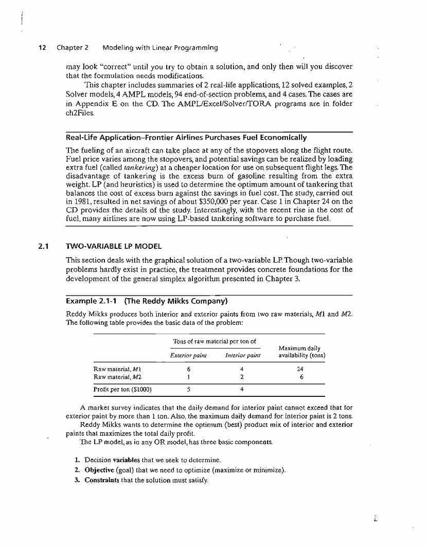
Example 2.1-1 (The Reddy Mikks Company)
Reddy Mikks produces both interior and exterior paints from two raw materials, Ml and M2.The following table provides the basic data of the problem:
Tons of raw material per ton of
Raw material, M1Raw material, M2
Profit per ton ($1000)
Exterior pain!
61
5
Interior paint
42
4
Maximum dailyavailability (tons)
246
A market survey indicates that the daily demand for interior paint cannot exceed that forexterior paint by more than 1 ton. Also, the maximum daily demand for interior paint is 2 tons.
Reddy Mikks wants to determine the optimum (best) product mix of interior and exteriorpaints that maximizes the total daily profit.
The LP model, as in any OR model, has three basic components.
1. Decision variables that we seek to determine.
2. Objective (goal) that we need to optimize (maximize or minimize).
3. Constraints that the solution must satisfy.
2.1 Two-Variable LP Model 13
The proper definition of the decision variables is an essential first step in the development of themodel. Once done, the task of constructing the objective function and the constraints becomesmore straightforward.
For the Reddy Mikks problem, we need to determine the daily amounts to be produced ofexterior and interior paints. Thus the variables of the model are defined as
Xl = Tons produced daily of exterior paint
X2 = Tons produced daily of interior paint
To construct the objective function, note that the company wants to maximize (i.e., increaseas much as possible) the total daily profit of both paints. Given that the profits per ton of exterior and interior paints are 5 and 4 (thousand) dollars, respectively, it follows that
Total profit from exterior paint = 5xl (thousand) dollars
Total profit from interior paint = 4X2 (thousand) dollars
Letting z represent the total daily profit (in thousands of dollars), the objective of the companyis
Maximize z = 5Xl + 4X2
Next, we construct the constraints that restrict raw material usage and product demand. Theraw material restrictions are expressed verbally as
(Usage of a raw material) ~ (MaXimum raw material)
by both paints availability
The daily usage of raw material MI is 6 tons per ton of exterior paint and 4 tons per ton of interior paint. Thus
Usage of raw material Ml by exterior paint = 6Xl tons/day
Usage of raw material Ml by interior paint = 4X2 tons/day
Hence
Usage of raw material Ml by both paints = 6Xt + 4x2 tons/day
In a similar manner,
Usage of raw material M2 by both paints = IXl + 2X2 tons/day
Because the daily availabilities of raw materials Ml and M2 are limited to 24 and 6 tons, respectively, the associated restrictions are given as
6Xt + 4X2 ~ 24
XI + 2X2::; 6
(Raw material MI)
(Raw material M2)
The first demand restriction stipulates that the excess of the daily production of interiorover exterior paint, X2 - Xl, should not exceed 1 ton, which translates to
(Market limit)
14 Chapter 2 Modeling with Linear Programming
The second demand restriction stipulates that the maximum daily demand of interior paint islimited to 2 tons, which translates to
X2 ~ 2 (Demand limit)
An implicit (or "understood-to-be") restriction is that variables Xl and X2 cannot assumenegative values. The nonnegativity restrictions, Xl ;:: 0, X2 ;:: 0, account for this requirement.
The complete Reddy Mikks model is
Maximize z = 5XI + 4X2
subject to
6xI + 4x2 ~ 24
XI + 2X2 ~ 6
-Xl + X2 ~ 1
x2 ~ 2
Xl> X2 C; 0
(1)
(2)
(3)
(4)
(5)
Any values of Xl and X2 that satisfy all five constraints constitute a feasible solution. Otherwise,the solution is infeasible. For example, the solution, Xl = 3 tons per day and X2 = I ton per day,is feasible because it does not violate any of the constraints, including the nonnegativity restrictions. To verify this result, substitute (Xl = 3, X2 = I) in the left-hand side of each constraint. Inconstraint (1) we have 6XI + 4X2 = 6 X 3 + 4 X 1 == 22, which is less than the right-hand sideof the constraint (= 24). Constraints 2 through 5 will yield similar conclusions (verify!). On theother hand, the solution Xl = 4 and X2 = 1 is infeasible because it does not satisfy constraint(I)-namely, 6 X 4 + 4 X 1 = 28, which is larger than the right-hand side (= 24).
The goal of the problem is to find the best feasible solution, or the optimum, that maximizes the total profit. Before we can do that, we need to know how many feasible solutions theReddy Mikks problem has. The answer, as we wiII see from the graphical solution in Section2.2, is "an infinite number," which makes it impossible to solve the problem by enumeration.Instead, we need a systematic procedure that will locate the optimum solution in a finite number of steps. The graphical method in Section 2.2 and its algebraic generalization in Chapter 3will explain how this can be accomplished.
Properties of the LP Model. In Example 2.1-1, the objective and the constraints areall linear functions. Linearity implies that the LP must satisfy three basic properties:
1. Proportionality: This property requires the contribution of each decisionvariable in both the objective function and the constraints to be directly proportional to the value of the variable. For example, in the Reddy Mikks model, thequantities 5Xl and 4X2 give the profits for producing Xl and X2 tons of exterior and interior paint, respectively, with the unit profits per ton, 5 and 4, providing the constantsof proportionality. If, on the other hand, Reddy Mikks grants some sort of quantity discounts when sales exceed certain amounts, then the profit will no longer be proportional to the production amounts, Xl and X2, and the profit function becomes nonlinear.
2. Additivity: This property requires the total contribution of all the variables inthe objective function and in the constraints to be the direct sum of the individualcontributions of each variable. In the Reddy Mikks model, the total profit equals the
2.2
2.2 GraphicallP Solution 15
sum of the two individual profit components. If, however, the two products compete formarket share in such a way that an increase in sales of one adversely affects the other,then the additivity property is not satisfied and the model is no longer linear.
3. Certainty: All the objective and constraint coefficients of the LP model are deterministic. This means that they are known constants-a rare occurrence in real life,where data are more likely to be represented by probabilistic distributions. In essence,LP coefficients are average-value approximations of the probabilistic distributions. Ifthe standard deviations of these distributions are sufficiently small, then the approximation is acceptable. Large standard deviations can be accounted for directly by usingstochastic LP algorithms (Section 19.2.3) or indirectly by applying sensitivity analysisto the optimum solution (Section 3.6).
PROBLEM SET 2.1A
1. For the Reddy Mikks model, construct each of the following constraints and express itwith a linear left-hand side and a constant right-hand side:
*(a) The daily demand for interior paint exceeds that of exterior paint by at least 1 ton.
(b) The daily usage of raw material M2 in tons is at most 6 and at least 3.
*(c) The demand for interior paint cannot be less than the demand for exterior paint.
(d) The minimum quantity that should be produced of both the interior and the exteriorpaint is 3 tons.
*(e) The proportion of interior paint to the total production of both interior and exteriorpaints must not exceed .5.
2. Determine the best feasible solution among the following (feasible and infeasible) solutions of the Reddy Mikks model:
(a) XI = 1, X2 = 4.
(b) Xl = 2, X2 = 2.
(c) XI = 3, x2 = 1.5.
(d) X I = 2, X2 = 1.
(e) XI = 2, X2 = -l.
*3. For the feasible solution XI = 2, x2 = 2 of the Reddy Mikks model, determine the unused amounts of raw materials Ml and M2.
4. Suppose that Reddy Mikks sells its exterior paint to a single wholesaler at a quantity discount.1l1e profit per ton is $5000 if the contractor buys no more than 2 tons daily and $4500otherwise. Express the objective function mathematically. Is the resulting function linear?
2.2 GRAPHICAL LP SOLUTION
The graphical procedure includes two steps:
1. Determination of the feasible solution space.2. Determination of the optimum solution from among all the feasible points in the
solution space.
The procedure uses two examples to show how maximization and minimizationobjective functions are handled.
16 Chapter 2 Modeling with Linear Programming
2.2.1 Solution of a Maximization ModeJ
Example 2.2-1
This example solves the Reddy Mikks model of Example 2.1-1.
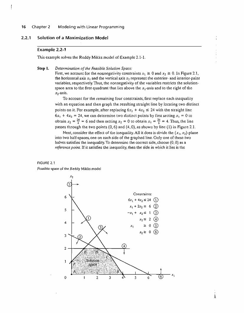
Step 1. Determination ofthe Feasible Solution Space:First, we account for the nonnegativity constraints Xl ~ 0 and X2 2: O. In Figure 2.1,the horizontal axis Xl and the vertical axis X2 represent the exterior- and interior-paintvariables, respectively. Thus, the nonnegativity of the variables restricts the solutionspace area to the first quadrant that lies above the xl-axis and to the right of thex2-axis.
To account for the remaining four constraints, first replace each inequality
with an equation and then graph the resulting straight line by locating two distinct
points on it. For example, after replacing 6x[ + 4X2 :::; 24 with the straight line
6xl + 4x2 = 24, we can determine two distinct points by first setting XI = 0 to
obtain X2 = ¥ = 6 and then setting X2 = 0 to obtain XI = ~ = 4. Thus, the line
passes through the two points (0,6) and (4,0), as shown by line (1) in Figure 2.1.Next, consider the effect of the inequality. All it does is divide the (xJ, x2)-plane
into two half-spaces, one on each side of the graphed line. Only one of these twohalves satisfies the inequality. To determine the correct side, choose (0,0) as areference point. If it satisfies the inequality, then the side in which it lies is the
FIGURE 2.1
Feasible space of the Reddy Mikks model
Constraints:6
CD6xI + 4x2:$ 24
Xl + 2x2 :$ 6 @5
CD-Xl + x2:$ 1
x2:$ 2 (1)4
@XI 2: 0
x22: 0 ®3
2
o
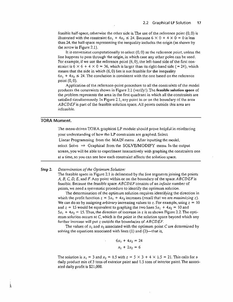
2.2 GraphicallP Solution 17
feasible half-space, otherwise the other side is. The use of the reference point (0,0) isillustrated with the constraint 6xI + 4xz :5 24. Because 6 x 0 + 4 x 0 = 0 is lessthan 24, the half-space representing the inequality includes the origin (as shown bythe arrow in Figure 2.1).
It is convenient computationally to select (0,0) as the reference point, unless theline happens to pass through the origin, in which case any other point can be used.For example, if we use the reference point (6,0), the left-hand side of the first constraint is 6 X 6 + 4 X 0 = 36, which is larger than its right-hand side (= 24), whichmeans that the side in which (6,0) lies is not feasible for the inequality6Xl + 4X2 :5 24. The conclusion is consistent with the one based on the referencepoint (0,0).
Application of the reference-point procedure to all the constraints of the modelproduces the constraints shown in Figure 2.1 (verify!). The feasible solution space ofthe problem represents the area in the first quadrant in which all the constraints aresatisfied simultaneously. In Figure 2.1, any point in or on the boundary of the areaABCDEF is part of the feasible solution space. All points outside this area areinfeasible.
TORA Moment.
The menu-driven TORA graphical LP module should prove helpful in reinforcingyour understanding of how the LP constraints are graphed. Select
Linear Programming from the MAIN menu. After inputting the model,
select Solve => Graphical from the SOLVE/MODIFY menu. In the output
screen, you will be able to experiment interactively with graphing the constraints one
at a time, so you can see how each constraint affects the solution space.
Step 2. Determination of the Optimum Solution:The feasible space in Figure 2.1 is delineated by the line segments joining the pointsA, B, C, D, E, and F. Any point within or on the boundary of the space ABCDEFisfeasible. Because the feasible space ABCDEF consists of an infinite number ofpoints, we need a systematic procedure to identify the optimum solution.
The determination of the optimum solution requires identifying the direction inwhich the profit function z = 5x1 + 4X2 increases (recall that we are maximizing z).We can do so by assigning arbitrary increasing values to z. For example, using z = 10and z = 15 would be equivalent to graphing the two lines 5Xl + 4X2 = 10 and5xI + 4x2 = 15. Thus, the direction of increase in z is as shown Figure 2.2. The optimum solution occurs at C, which is the point in the solution space beyond which anyfurther increase will put z outside the boundaries of A BCDEF.
The values of Xl and X2 associated with the optimum point C are determined bysolving the equations associated with lines (1) and (2)-that is,
6X1 + 4X2 = 24
Xl + 2X2 = 6
The solution is Xl = 3 and x2 = 1.5 with z = 5 X 3 + 4 X 1.5 = 21. 111is calls for adaily product mix of 3 tons of exterior paint and 1.5 tons of interior paint. The associated daily profit is $21,000.
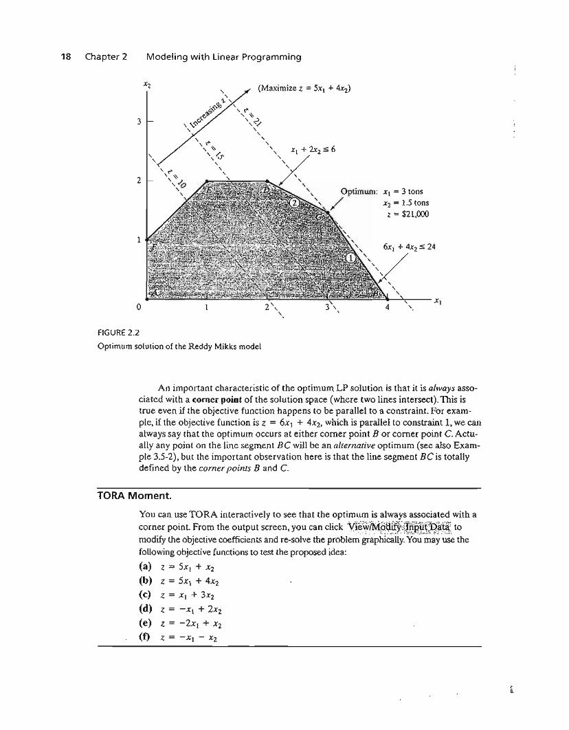
18 Chapter 2 Modeling with Linear Programming
(Maximize z = 5Xl + 4x2)
3
2
1
o
,,
2',,
, Optimum: Xl = 3 tons
>l< / x2 = 1.5 tonsZ = $21,000
==4-~,:---- Xl
4 '
FIGURE 2.2
Optimum solution of the Reddy Mikks model
An important characteristic of the optimum LP solution is that it is always associated with a cornel" point of the solution space (where two lines intersect). This istrue even if the objective function happens to be parallel to a constraint. For example, if the objective function is z = 6XI + 4X2, which is parallel to constraint I, we canalways say that the optimum occurs at either corner point B or comer point C. Actually any point on the line segment BC will be an alternative optimum (see also Example 3.5-2), but the important observation here is that the line segment BC is totallydefined by the corner points Band C.
TORA Moment.
You can use TORA interactively to see that the optimum is always associated with a
corner point. From the output screen, you can clickYi~~i¥A~N~l~~¥~~B~~; tomodify the objective coefficients and re-solve the problem graphically. You may use thefollowing objective functions to test the proposed idea:
(a) z = 5xI + X2
(b) Z = 5Xl + 4X2
(c) Z = Xl + 3x2
(d) Z = -Xl + 2X2
(e) z = - 2xl + Xl
(f) Z = -XI - X2
i.1;.
2.2 Graphical LP Solution 19
The observation that the LP optimum is always associated with a corner point means thatthe optimum solution can be found simply by enumerating all the corner points as the followingtable shows:
Corner point (Xl> X2) Z
A (0,0) 0B (4,0) 20C (3,1.5) 21 (OPTIMUM)D (2,2) 18E (1,2) 13F (0,1) 4
As the number of constraints and variables increases, the number of corner points also increases, and the proposed enumeration procedure becomes less tractable computationally. Nevertheless, the idea shows that, from the standpoint of determining the LP optimum, thesolution space ABCDEF with its infinite number of solutions can, in fact, be replaced with afinite number of promising solution points-namely, the corner points, A, B, C, D, E, and F. Thisresult is key for the development of the general algebraic algorithm, called the simplexmethod, which we will study in Chapter 3.
PROBLEM SET 2.2A
1. Determine the feasible space for each of the following independent constraints, giventhat Xl, X2 :::: O.
*(a) - 3XI + X2 5; 6.
(b) Xl - 2X2 :::: 5.
(c) 2Xl - 3X2 5; 12.
*(d) XI - X2 5; O.
(e) -Xl + X2 :::: O.
2. Identify the direction of increase in z in each of the following cases:
*(a) Maximize z = Xl - X2'
(b) Maximize z = - 5x I - 6X2'
(c) Maximize z = -Xl + 2X2'
*(d) Maximize z = -3XI + X2'
3. Determine the solution space and the optimum solution of the Reddy Mikks model foreach of the following independent changes:
(a) The maximum daily demand for exterior paint is at most 2.5 tons.
(b) The daily demand for interior paint is at least 2 tons.
(c) The daily demand for interior paint is exactly 1 ton higher than that for exteriorpaint.
(d) The daily availability of raw material Ml is at least 24 tons.
(e) The daily availability of raw material Ml is at least 24 tons, and the daily demand forinterior paint exceeds that for exterior paint by at least 1 ton.
20 Chapter 2 Modeling with Linear Programming
4. A company that operates 10 hours a day manufactures two products on three sequentialprocesses. TIle following table summarizes the data of the problem:
Minutes per unit
Product
12
Process 1
105
Process 2
620
Process 3
810
Unit profit
$2$3
Determine the optimal mix of the two products.
*5. A company produces two products, A and B. The sales volume for A is at least 80% ofthe total sales of both A and B. However, the company cannot sell more than 100 units ofA per day. Both products use one raw material, of which the maximum daily availabilityis 240 lb. The usage rates of the raw material are 2 lb per unit of A and 4 lb per unit of B.TIle profit units for A and Bare $20 and $50, respectively. Determine the optimal product mix for the company.
6. Alumco manufactures aluminum sheets and aluminum bars. The maximum productioncapacity is estimated at either 800 sheets or 600 bars per day. The maximum daily demand is 550 sheets and 580 bars. The profit per ton is $40 per sheet and $35 per bar. Determine the optimal daily production mix.
*7. An individual wishes to invest $5000 over the next year in two types of investment: Investment A yields 5% and investment B yields 8%. Market research recommends an allocation of at least 25% in A and at most 50% in B. Moreover, investment in A should be atleast half the investment in B. How should the fund be allocated to the two investments?
8. The Continuing Education Division at the Ozark Community College offers a total of30 courses each semester. The courses offered are usually of two types: practical, suchas woodworking, word processing, and car maintenance; and humanistic, such as history, music, and fine arts. To satisfy the demands of the community, at least 10 courses ofeach type must be offered each semester. The division estimates that the revenues ofoffering practical and humanistic courses are approximately $1500 and $1000 percourse, respectively.
(a) Devise an optimal course offering for the college.
(b) Show that the worth per additional course is $1500, which is the same as the revenueper practical course. What does this result mean in terms of offering additionalcourses?
9. ChemLabs uses raw materials I and II to produce two domestic cleaning solutions, Aand B. The daily availabilities of raw materials I and II are 150 and 145 units, respectively.One unit of solution A consumes .5 unit of raw materiall and .6 unit of raw material II,and one unit of solution Buses .5 unit of raw materiall and .4 unit of raw materiaill. Theprofits per unit of solutions A and Bare $8 and $10, respectively. The daily demand forsolution A lies between 30 and 150 units, and that for solution B between 40 and 200units. Find the optimal production amounts of A and B.
10. In the Ma-and-Pa grocery store, shelf space is limited and must be used effectively to increase profit. Two cereal items, Grano and Wheatie, compete for a total shelf space of60 ft2. A box of Grano occupies.2 ft2 and a box ofWheatie needs .4 ft2. The maximumdaily demands of Grano and Wheatie are 200 and 120 boxes, respectively. A box ofqrano nets $1.00 in profit and a box of Wheatie $1.35. Ma-and-Pa thinks that because theunit profit ofWheatie is 35% higher than that of Grano, Wheatie should be allocated
2.2 GraphicallP Solution 21
35% more space than Grano, which amounts to allocating about 57% to Wheatie and43% to Grano. What do you think?
11. Jack is an aspiring freshman at Diem University. He realizes that "all work and no playmake Jack a dull boy." As a result, Jack wants to apportion his available time of about10 hours a day between work and play. He estimates that play is twice as much fun aswork. He also wants to study at least as much as he plays. However, Jack realizes that ifhe is going to get all his homework assignments done, he cannot play more than 4hours a day. How should Jack allocate his time to maximize his pleasure from bothwork and play?
12. Wild West produces two types of cowboy hats. A type 1 hat requires twice as much labortime as a type 2. If the all available labor time is dedicated to Type 2 alone, the companycan produce a total of 400 Type 2 hats a day. The respective market limits for the twotypes are 150 and 200 hats per day. The profit is $8 per Type 1 hat and $5 per Type 2 hat.Determine the number of hats of each type that would maximize profit.
13. Show & Sell can advertise its products on local radio and television (TV). The advertisingbudget is limited to $10,000 a month. Each minute of radio advertising costs $15 and eachminute ofTY commercials $300. Show & Sell likes to advertise on radio at least twice asmuch as on TV. In the meantime, it is not practical to use more than 400 minutes of radioadvertising a month. From past experience, advertising on TV is estimated to be 25 timesas effective as on radio. Determine the optimum allocation of the budget to radio and TVadvertising.
*14. Wyoming Electric Coop owns a steam-turbine power-generating plant. BecauseWyoming is rich in coal deposits, the plant generates its steam from coal. 111is, however,may result in emission that does not meet the Environmental Protection Agency standards. EPA regulations limit sulfur dioxide discharge to 2000 parts per million per ton ofcoal burned and smoke discharge from the plant stacks to 20 lb per hour. The Coop receives two grades of pulverized coal, C1 and C2, for use in the steam plant. The twogrades are usually mixed together before burning. For simplicity, it can be assumed thatthe amount of sulfur pollutant discharged (in parts per million) is a weighted average ofthe proportion of each grade used in the mixture. The following data are based on consumption of 1 ton per hour of each of the two coal grades.
Sulfur discharge Smoke discharge Steam generatedCoal grade in parts per million in Ib per hour in lb per hour
Cl 1800 2.1 12,000C2 2100 .9 9,000
(a) Determine the optimal ratio for mixing the two coal grades.
(b) Determine the effect of relaxing the smoke discharge limit by 1 lb on the amount ofgenerated steam per hour.
15. Top Toys is planning a new radio and TV advertising campaign. A radio commercial costs$300 and a TV ad cosls $2000. A total budget of $20,000 is allocated to the campaign.However, to ensure that each medium will have at least one radio commercial and oneTV ad, the most that can be allocated to either medium cannot exceed 80% of the totalbudget. It is estimated that the first radio commercial will reach 5000 people, with eachadditional commercial reaching only 2000 new ones. For TV, the first ad will reach 4500people and each additional ad an additional 3000. How should the budgeted amount beallocated between radio and TV?
22 Chapter 2 Modeling with Linear Programming
16. The Burroughs Garment Company manufactures men's shirts and women's blouses forWalmark Discount Stores. Walmark will accept all the production supplied by Burroughs.The production process includes cutting, sewing, and packaging. Burroughs employs 25workers in the cutting department, 35 in the sewing department, and 5 in the packagingdepartment. The factory works one 8-hour shift, 5 days a week. The following table givesthe time requirements and profits per unit for the two garments:
Minutes per unit
Garment
ShirtsBlouses
Cutting
2060
Sewing
7060
Packaging
124
Unit profit ($)
812
Determine the optimal weekly production schedule for Burroughs.
17. A furniture company manufactures desks and chairs. The sawing department cuts thelumber for both products, which is then sent to separate assembly departments. Assembled items are sent for finishing to the painting department. The daily capacity of thesawing department is 200 chairs or 80 desks. TIle chair assembly department can produce120 chairs daily and the desk assembly department 60 desks daily. TIle paint departmenthas a daily capacity of either 150 chairs or 110 desks. Given that the profit per chair is $50and that of a desk is $100, determine the optimal production mix for the company.
*18. An assembly line consisting of three consecutive stations produces two radio models: HiFi1 and HiFi-2. The following table provides the assembly times for the three workstations.
Minutes per unit
Workstation
123
HiFi-1
654
HiFi-2
456
2.The daily maintenance for stations 1,2, and 3 consumes 10%,14%, and 12%, respectively, of the maximum 480 minutes available for each station each day. Determine the optimal product mix that will minimize the idle (or unused) times in the three workstations.
19. TORA Experiment. Enter the following LP into TORA and select the graphic solutionmode to reveal the LP graphic screen.
Minimize z = 3x I + 8Xl
subject to
XI + Xl ~ 82xI - 3xz s 0
Xl + 2X2 S 303x\ - X2 ~ 0
Xl S 10Xz ~ 9
Xl> X2 ~ 0
Next, on a sheet of paper, graph and scale the xI- and xraxes for the problem (you mayalso click Print Graph on the top of the right window to obtain a ready-to-use scaled
2.2 Graphical LP Solution 23
sheet). Now, graph a constraint manually on the prepared sheet, then click it on the leftwindow of the screen to check your answer. Repeat the same for each constraint andthen terminate the procedure with a graph of the objective function. The suggestedprocess is designed to test and reinforce your understanding of the graphical LP solutionthrough immediate feedback from TORA.
20. TORA Experiment. Consider the following LP model:
Maximize z = 5xI + 4X2
subject to
6xI + 4X2 ::; 246x1 + 3X2 ::; 22.5
XI + X2::; 5XI + 2X2::; 6
- XI + X2::; 1xz::; 2
XJ, X2 ~ 0
In LP, a constraint is said to be redundant if its removal from the model leaves the feasible solution space unchanged. Use the graphical facility ofTORA to identify the redundant constraints, then show that their removal (simply by not graphing them) does notaffect the solution space or the optimal solution.
21. TORA Experiment. In the Reddy Mikks model, use TORA to show that the removal ofthe raw material constraints (constraints 1 and 2) would result in an unbounded solutionspace. What can be said in this case about the optimal solution of the model?
22. TORA Experiment. In the Reddy Mikks model, suppose that the following constraint isadded to the problem.
X2 ~ 3
Use TORA to show that the resulting model has conflicting constraints that cannot besatisfied simultaneously and hence it has no feasible solution.
2.2.2 Solution of a Minimization Model
Example 2.2-2 (Diet Problem)
Ozark Farms uses at least 800 lb of special feed daily. The special feed is a mixture of corn andsoybean meal with the following compositions:
Ib per Ib of feedstuff
Feedstuff
CornSoybean meal
Protein
.09
.60
Fiber
.02
.06
Cost ($/Ib)
.30
.90
The dietary requirements of the special feed are at least 30% protein and at most 5% fiber.Ozark Farms wishes to determine the daily minimum-cost feed mix.
Because the feed mix consists of corn and soybean meal, the decision variables of the modelare defined as
Xl = lb of corn in the daily mix
x2 = lb of soybean meal in the daily mix

24 Chapter 2 Modeling with Linear Programming
The objective function seeks to minimize the total daily cost (in dollars) of the feed mix and isthus expressed as
Minimize z = .3xl + .9x2
The constraints of the model reflect the daily amount needed and the dietary requirements.Because Ozark Farms needs at least 800 Ib of feed a day, the associated constraint can be expressed as
XI + X2 ~ 800
As for the protein dietary requirement constraint, the amount of protein included in Xl lb ofcorn and X2 lb of soybean meal is (.09Xl + .6X2) lb. This quantity should equal at least 30% ofthe total feed mix (Xl + X2) lb-that is,
.09xl + .6X2 ~ .3(XI + X2)
In a similar manner, the fiber requirement of at most 5% is constructed as
.02xl + .06X2 ~ .05(xl + X2)
The constraints are simplified by moving the terms in XI and X2 to the left-hand side of eachinequality, leaving only a constant on the right-hand side. The complete model thus becomes
minimize z = .3XI + .9X2
subject to
XI + X2 ~ 800
.21xl - .30x2 ~ 0
.03x I - .Olx2 ~ 0
Figure 2.3 provides the graphical solution of the model. Unlike those of the Reddy Mikksmodel (Example 2.2-1), the second and third constraints pass through the origin. To plot theassociated straight lines, we need one additional point, which can be obtained by assigning avalue to one of the variables and then solving for the other variable. For example, in the second constraint, Xl = 200 will yield .21 x 200 - .3x2 = 0, or X2 = 140. This means that thestraight line .21xl - .3x2 = 0 passes through (0,0) and (200,140). Note also that (0,0) cannot beused as a reference point for constraints 2 and 3, because both lines pass through the origin. Instead, any other point [e.g., (100, 0) or (0,100)] can be used for that purpose.
Solution:
Because the present model seeks the minimization of the objective function, we need to reducethe value of z as much as possible in the direction shown in Figure 2.3. The optimum solution is theintersection of the two lines XI + X2 = 800 and .21xl - .3X2 = 0, which yields Xl = 470.591b andX2 = 329.41 lb. The associated minimum cost of thefeed mix is z = .3 X 470.59 + .9 x 329.42 =$437.65 per day.
Remarks. We need to take note of the way the constraints of the problem are constructed. Because the model is minimizing the total cost, one may argue that the solution will seek exactly800 tons of feed. Indeed, this is what the optimum solution given above does. Does this meanthen that the first constraint can be deleted altogether simply by including the amount 800 tons
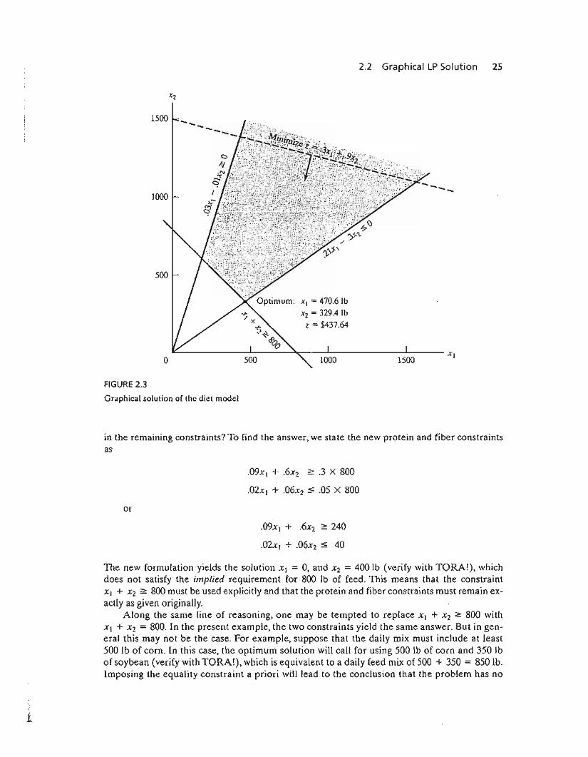
FIGURE 2.3
1500
1000
500
2.2 Graphical LP Solution 25
--
Xl = 470.61b
X2 = 329.41bz = $437.64
~ -'---- ~__...1..- -'- Xl
1500
Graphical solution of the diet model
in the remaining constraints? To find the answer, we state the new protein and fiber constraintsas
.09XI + .6X2 ~.3 X SOD
.02XI + .06X2 :5 .05 X SOO
or
.09Xl + .6X2 ~ 240
.02Xt + .06X2:5 40
The new formulation yields the solution XI = 0, and X2 = 400 lb (verify with TORA!), whichdoes not satisfy the implied requirement fOT SOO Ib of feed. This means that the constraintXI + X2 ~ 800 must be used explicitly and that the protein and fiber constraints must remain exaClly as given originally.
Along the same line of reasoning, one may be tempted to replace XI + X2 ;:::: 800 withXI + X2 = 800. In the present example, the two constraints yield the same answer. But in general this may not be the case. For example, suppose that the daily mix must include at least500 lb of corn. In this case, the optimum solution will call for using 500 lb of corn and 350 Ibof soybean (verify with TORA!), which is equivalent to a daily feed mix of 500 + 350 = 850 lb.Imposing the equality constraint a priori will lead to the conclusion that the problem has no
26 Chapter 2 Modeling with Linear Programming
feasible solution (verify with TORA!). On the other hand, the use of the inequality is inclusiveof the equality case, and hence its use does not prevent the model from producing exactly 800 Ibof feed mix, should the remaining constraints allow it. TI1e conclusion is that we should not "preguess" the solution by imposing the additional equality restriction, and we should always use inequalities unless the situation explicitly stipulates the use of equalities.
PROBLEM SET 2.2B
1. Identify the direction of decrease in z in each of the following cases:
*(a) Minimize z = 4xI - 2x2'
(b) Minimize z = -3xl + X2'
(c) Minimize z = -Xl - 2X2'
2. For the diet model, suppose that the daily availability of corn is limited to 450 lb. Identifythe new solution space, and determine the new optimum solution.
3. For the diet model, what type of optimum solution would the model yield if the feed mixshould not exceed 800 Ib a day? Does the solution make sense?
4. John must work at least 20 hours a week to supplement his income while attendingschool. He has the opportunity to work in two retail stores. In store 1, he can work between 5 and 12 hours a week, and in store 2 he is allowed between 6 and 10 hours. Bothstores pay the same hourly wage. In deciding how many hours to work in each store, Johnwants to base his decision on work stress. Based on interviews with present employees,John estimates that, on an ascending scale of 1 to 10, the stress factors are 8 and 6 atstores 1 and 2, respectively. Because stress mounts by the hour, he assumes that the totalstress for each store at the end of the week is proportional to the number of hours heworks in the store. How many hours should 10hn work in each store?
*5. OilCo is building a refinery to produce four products: diesel, gasoline, lubricants, and jetfuel. The minimum demand (in bblJday) for each of these products is 14,000,30,000,10,000, and 8,000, respectively. Iran and Dubai are under contract to ship crude to OilCo.Because of the production quotas specified by OPEC (Organization of Petroleum Exporting Countries) the new refinery can receive at least 40% of its crude from Iran andthe remaining amount from Dubai. OilCo predicts that the demand and crude oil quotaswill remain steady over the next ten years.
The specifications of the two crude oils lead to different product mixes: One barrelof Iran crude yields .2 bbl of diesel, .25 bbl of gasoline,.l bbl of lubricant, and .15 bbl ofjet fuel. The corresponding yields from Dubai crude are .1, .6, .15, and .1, respectively.Oileo needs to determine the minimum capacity of the refinery (in bbll day).
6. Day Trader wants to invest a sum of money that would generate an annual yield of atleast $10,000. Two stock groups are available: blue chips and high tech, with average annual yields of 10% and 25%, respectively. TIlOugh high-tech stocks provide higher yield,they are more risky, and Trader wants to limit the amount invested in these stocks to nomore than 60% of the total investment. What is the minimum amount Trader should invest in each stock group to accomplish the investment goal?
*7. An industrial recycling center uses two scrap aluminum metals, A and B, to produce aspecial alloy. Scrap A contains 6% aluminum, 3% silicon, and 4% carbon. Scrap B has3% aluminum, 6% silicon, and 3% carbon.The costs per ton for scraps A and Bare $100and $80, respectively. TIle specifications of the special alloy require that (1) the aluminumcontent must be at least 3% and at most 6%, (2) the silicon content must lie between 3%
2.
2.
2.3 Selected lP Applications 27
and 5%, and (3) the carbon content must be between 3% and 7%. Determine the optimum mix of the scraps that should be used in producing 1000 tons of the alloy.
8. TORA Experiment. Consider the Diet Model and let the objective function be given as
Minimize z = .8x1 + .8X2
Use TORA to show that the optimum solution is associated with two distinct cornerpoints and that both points yield the same objective value. In this case, the problem issaid to have alternative optima. Explain the conditions leading to this situation and showthat, in effect, the problem has an infinite number of alternative optima, then provide aformula for determining all such solutions.
2.3 SELECTED LP APPLICATIONS
This section presents realistic LP models in which the definition of the variablesand the construction of the objective function and constraints are not as straightforward as in the case of the two-variable model. The areas covered by these applications include the following:
1. Urban planning.2. Currency arbitrage.3. Investment.4. Production planning and inventory control.S. Blending and oil refining.6. Manpower planning.
Each model is fully developed and its optimum solution is analyzed and interpreted.
2.3.1 Urban Planning 1
Urban planning deals with three general areas: (1) building new housing developments, (2) upgrading inner-city deteriorating housing and recreational areas, and (3)planning public facilities (such as schools and airports). The constraints associated withthese projects are both economic (land, construction, financing) and social (schools,parks, income level). The objectives in urban planning vary. [n new housing developments, profit is usually the motive for undertaking the project. In the remaining twocategories, the goals involve social, political, economic, and cultural considerations. Indeed, in a publicized case in 2004, the mayor of a city in Ohio wanted to condemn anold area of the city to make way for a luxury housing development. The motive was toincrease tax collection to help alleviate budget shortages. The example presented inthis section is fashioned after the Ohio case.
IThis section is based on Laidlaw (1972).
28 Chapter 2 Modeling with Linear Programming
Example 2.3-1 (Urban Renewal Model)
The city of Erstville is faced with a severe budget shortage. Seeking a long-term solution, the citycouncil votes to improve the tax base by condemning an inner-city housing area and replacing itwith a modern development.
The project involves two phases: (1) demolishing substandard houses to provide land forthe new development, and (2) building the new development. The following is a summary of thesituation.
1. As many as 300 substandard houses can be demolished. Each house occupies a 25-acrelot. The cost of demolishing a condemned house is $2000.
2. Lot sizes for new single-, double-, triple-, and quadruple-family homes (units) are .18, .28,A, and.5 acre, respectively. Streets, open space, and utility easements account for 15% ofavailable acreage.
3. In the new development the triple and quadruple units account for at least 25% of thetotal. Single units must be at least 20% of all units and double units at least 10%.
4. TIle tax levied per unit for single, double, triple, and quadruple units is $1,000, $1,900,$2,700, and $3,400, respectively.
5. The construction cost per unit for single-, double-, triple-, and quadruple- family homes is$50,000, $70,000, $130,000, and $160,000, respectively. Financing through a local bank canamount to a maximum of $15 million.
How many units of each type should be constructed to maximize tax collection?
Mathematical Model: Besides determining the number of units to be constructed of each typeof housing, we also need to decide how many houses must be demolished to make room for thenew development. TIlus, the variables of the problem can be defined as follows:
Xl = Number of units of single-family homes
X2 = Number of units of double-family homes
X3 = Number of units of triple-family homes
X4 = Number of units of quadruple-family homes
Xs = Number of old homes to be demolished
The objective is to maximize total tax collection from all four types of homes-that is,
Maximize z = 1000xl + 1900x2 + 2700X3 + 3400X4
The first constraint of the problem deals with land availability.
(Acreage used for. new) "$ (Net available)
home constructIOn acreage
From the data of the problem we have
Acreage needed for new homes = .18xl + .28x2 + AX3 + .5X4
2.3 Selected LP Applications 29
To determine the available acreage, each demolished home occupies a .25-acre lot, thus netting.25x5 acres. Allowing for 15% open space, streets, and easements, the net acreage available is.85(.25x5) = .2125x5' The resulting constraint is
:5 .2125x5
or
.18x1 + .28x2 + .4x3 + .5X4 - .2125x5 :5 0
The number of demolished homes cannot exceed 300, which translates to
X5 :5 300
Next we add the constraints limiting the number of units of each home type.
(Number of single units) ;::: (20% of all units)
(Number of double units) ;::: (10% of all units)
(Number of triple and quadruple units) ;::: (25% of all units)
These constraints translate mathematically to
XI ;::: .2(Xl + x2 + x3 + X4)
X2 ;::: .1(x1 + X2 + x3 + X4)
X3 + X4 ;::: .25(Xl + X2 + X3 + X4)
TIle only remaining constraint deals with keeping the demolishition/construction cost within theallowable budget-that is,
(Construction and demolition cost) :5 (Available budget)
Expressing all the costs in thousands of dollars, we get
The complete model thus becomes
Maximize z = IOOOxl + 19OOx2 + 2700x3 + 34OOX4
subject to
.18xl + .28X2 + .4x3 + .5X4 - .2125x5 :5 0
X5 :5 300
- .8Xl + .2X2 + .2X3 + .2X4
.lx( - .9x2 + .lx3 + .lx4
.25xl + .25x2 - .75x} - .75x4
:50
:50
:50
50Xl + 70x2 + 130x3 + 160x4 + 2X5 :5 15000
30 Chapter 2 Modeling with Linear Programming
Solution:
The optimum solution (using file ampIEX2.3-1.txt or solverEx2.3-l.xls) is:
Total tax collection = z = $343,965Number of single homes = XI = 35.83 :::" 36 unitsNumber of double homes = X2 = 98.53 :::" 99 unitsNumber of triple homes = X3 = 44.79 :::" 45 unitsNumber of quadruple homes = X4 ::; 0 unitsNumber of homes demolished = Xs = 244.49 ~ 245 units
Remarks. Linear programming does not guarantee an integer solution automatically, and thisis the reason for rounding the continuous values to the closest integer.llle rounded solution callsfor constructing 180 (= 36 + 99 + 45) units and demolishing 245 old homes, which yields$345,600 in taxes. Keep in mind, however, that, in general, the rounded solution may not be feasible. In fact, the current rounded solution violates the budget constraint by $70,000 (verify!). Interestingly, the true optimum integer solution (using the algorithms in Chapter 9) isXl = 36, X2 = 98, X3 = 45, X4 = 0, and Xs = 245 with z = $343,700. Carefully note that therounded solution yields a better objective value, which appears contradictory. The reason is thatthe rounded solution calls for producing an extra double home, which is feasible only if the budget is increased by $70,000.
PROBLEM SET 2.3A
1. A realtor is developing a rental housing and retail area. TIle housing area consists of efficiency apartments, duplexes, and single-family homes. Maximum demand by potentialrenters is estimated to be 500 efficiency apartments, 300 duplexes, and 250 single-familyhomes, but the number of duplexes must equal at least 50% of the number of efficiencyapartments and single homes. Retail space is proportionate to the number of home unitsat the rates of at least 10 ft2
, 15 ft2, and 18 ft2 for efficiency, duplex, and single family
units, respectively. However, land availability limits retail space to no more than10,000 ft2. The monthly rental income is estimated at $600, $750, and $1200 for efficiency-,duplex-, and single-family units, respectively. The retail space rents for $1001ft2. Determinethe optimal retail space area and the number of family residences.
2. TIle city council of Fayetteville is in the process of approving the construction of a new200,000-ft2 convention center. Two sites have been proposed, and both require exercisingthe "eminent domain" law to acquire the property. The following table provides dataabout proposed (contiguous) properties in both sites together with the acquisition cost.
Site 1 Site 2
Property Area (1000 ft2) Cost (1000 $) Area (1000 ft2) Cost (1000 $)
1 20 1,000 80 2,8002 50 2,100 60 1,9003 50 2,350 50 2,8004 30 1,850 70 2,5005 60 2,950
Partial acquisition of property is allowed. At least 75% of property 4 must be acquiredif site 1 is selected, and at least 50% of property 3 must be acquired if site 2 is selected.
this:alls~Ids
fea.In) isthe
thatmd-
:ffi-
lycylits
cy-,nine
2.3 Selected LP Applications 31
Although site 1 property is more expensive (on a per fe basis), the construction cost isless than at site 2, because the infrastructure at site 1 is in a much better shape. COIl
struction cost is $25 million at site 1 and $27 million at site 2. Which site should be selected, and what properties should be acquired?
*3. A city will undertake five urban renewal housing projects over the next five years. Eachproject has a different starting year and a different duration. The following table providesthe basic data of the situation:
Cost Annual incomeYear 1 Year 2 Year 3 Year 4 Year 5 (million $) (million $)
Project 1 Start End 5.0 .05Project 2 Start End 8.0 .07Project 3 Start End 15.0 .15Project 4 Start End 1.2 .02Budget (million $) 3.0 6.0 7.0 7.0 7.0
Projects 1 and 4 must be finished completely within their durations. The remaining two projects can be finished partially within budget limitations, if necessary. However, each projectmust be at least 25% completed within its duration. At the end of each year, the completedsection of a project is immediately occupied by tenants and a proportional amount of income is realized. For example, if 40% of project 1 is completed in year 1 and 60% in year3, the associated income over the five-year planning horizon is .4 X $50,000(for year 2) + .4 X $50,000 (for year 3) + (.4 + .6) X $50,000 (for year 4) +(.4 + .6) X $50,000 (for year 5) = (4 X .4 + 2 X .6) X $50,000. Determine the optimal schedule for the projects that will maximize the total income over the five-yearhorizon. For simplicity, disregard the time value of money.
4. The city of Fayetteville is embarking on an urban renewal project that will include lowerand middle-income row housing, upper-income luxury apartments, and public housing.The project also includes a public elementary school and retail facilities. The size of theelementary school (number of classrooms) is proportional to the number of pupils, andthe retail space is proportional to the number of housing units. The following table provides the pertinent data of the situation:
IV
iing
s1.
Lower Middle Upper Publicincome income income housing
Minimum number of units 100 125 75 300Maximum number of units 200 190 260 600Lot size per unit (acre) .05 .07 .03 .025Average number of pupils per unil 1.3 1.2 .5 1.4Retail demand per unit (acre) .023 .034 .046 .023Annual income per unit($) 7000 12,000 20,000 5000
School Retailroom unit
o2S
.045 .1
.03415,000
!redted.
The new school can occupy a maximum space of 2 acres at the rate of at most 25 pupilsper room. TIle operating annual cost per school room is $10,000. The project will be located on a 50-acre vacant property owned by the city. Additionally, the project can make useof an adjacent property occupied by 200 condemned slum homes. Each condemned homeoccupies .25 acre. The cost of buying and demolishing a slum unit is $7000. Open space,streets, and parking lots consume 15% of total available land.
Develop a linear program to determine the optimum plan for the project.
32 Chapter 2 Modeling with Linear Programming
5. Realco owns 800 acres of undeveloped land on a scenic lake in the heart of the OzarkMountains. In the past, little or no regulation was imposed upon new developmentsaround the lake. The lake shores are now dotted with vacation homes, and septic tanks,most of them improperly installed, are in extensive use. Over the years, seepage from theseptic tanks led to severe water pollution. To curb further degradation of the lake, countyofficials have approved stringent ordinances applicable to all future developments: (1)Only single-, double-, and triple-family homes can be constructed, with single-familyhomes accounting for at least 50% of the total. (2) To limit the number of septic tanks,minimum lot sizes of 2, 3, and 4 acres are required for single-, double-, and triple-familyhomes, respectively. (3) Recreation areas of 1 acre each must be established at the rate ofone area per 200 families. (4) To preserve the ecology of the lake, underground watermay not be pumped out for house or garden use. The president of Realco is studying thepossibility of developing the 800-acre property. The new development will include single-,double-, and triple-family homes. It is estimated that 15% of the acreage will be allocatedto streets and utility easements. Realco estimates the returns from the different housinguni ts as follows:
Housing unit
Net return per unit ($)
Single
10,000
Double
12,000
Triple
15,000
The cost of connecting water service to the area is proportionate to the number ofunits constructed. However, the county charges a minimum of $100,000 for the project. Additionally, the expansion of the water system beyond its present capacity islimited to 200,000 gallons per day during peak periods. The following data summarizethe water service connection cost as well as the water consumption, assuming an average size family:
Housing unit
Water service connection cost per unit ($)Water consumption per unit (gal/day)
Single Double
1000 1200400 600
Triple Recreation
1400 800840 450
Develop an optimal plan for Realco.
6. Consider the Realco model of Problem 5. Suppose that an additional 100 acres of landcan be purchased for $450,000, which will increase the total acreage to 900 acres. Is this aprofitable deal for Realco?
2.3.2 Currency Arbitrage2
In today's global economy, a multinational company must deal with currencies of thecountries in which it operates. Currency arbitrage, or simultaneous purchase and saleof currencies in different markets, offers opportunities for advantageous movement ofmoney from one currency to another. For example, converting £1000 to U.S. dollars in2001 with an exchange rate of $1.60 to £1 will yield $1600. Another way of making theconversion is to first change the British pound to Japanese yen and then convert the yento U.S. dollars using the 2001 exchange rates of £1 = ¥175 and $1 = ¥105. The
2This section is based on J. Kornbluth and G. Salkin (1987,'Chapter 6).
,t
2.3 Selected LP Applications 33
(£1,000 x ¥175)resulting dollar amount is ¥105 = $1,666.67. This example demonstrates
the advantage of converting the British money first to Japanese yen and then to dollars. This section shows how the arbitrage problem involving many currencies can beformulated and solved as a linear program.
Example 2.3-2 (Curr~ncy Arbitrage Model)
Suppose that a company has a total of 5 million dollars that can be exchanged for euros (€),British pounds (£), yen (¥), and Kuwaiti dinars (KD). Currency dealers set the following limitson the amount of any single transaction: 5 million dollars, 3 million euros, 3.5 million pounds,100 million yen, and 2.8 million KDs. The table below provides typical spot exchange rates. Thebottom diagonal rates are the reciprocal of the top diagonal rates. For example, rate(€~ $) =lIrate( $~ €) = 1/.769 = 1.30.
$ € £ ¥ KD
$ 1 .769 .625 105 .342
€ 1 1 .813 137 .445.769
£ 1 I 1 169 .543.625 ,8JJ
¥ I I -.L 1 .0032105 137 169
KD 1 J -.L 1 1.342 .445 .543 ,0032
Is it possible to increase the dollar holdings (above the initial $5 million) by circulating currencies through the currency market?
Mathematical Model: The situation starts with $5 million. This amount goes through a number ofconversions to other currencies before ultimately being reconverted to dollars. The problem thusseeks determining the amount of each conversion that will maximize the total dollar holdings.
For the purpose of developing the model and simplifying the notation, the following numeric code is used to represent the currencies.
Define
Currency
Code
$
1
€
2
£
3
¥
4
KD
5
Xij = Amount in currency i converted to currency j, i and j = 1,2, ... ,5
For example, Xl2 is the dollar amount converted to euros and XSI is the KD amount converted todollars. We further define two additional variables representing the input and the output of thearbitrage problem:
I = Initial dollar amount (= $5 million)
y = Final dollar holdings (to be determined from the solution)
Our goal is to determine the maximum final dollar holdings, y, subject to the currency flow restrictions and the maximum limits allowed for the different transactions.
34 Chapter 2
FIGURE 2.4
Modeling with Linear Programming
.625x13
Definition of the input/output variable, XI}, between $ and £
We start by developing the constraints of the model. Figure 2.4 demonstrates the idea ofconverting dollars to pounds. The dollar amount XI3 at originating currency 1 is converted to.625xl3 pounds at end currency 3.At the same time, the transacted dollar amount cannot exceedthe limit set by the dealer, Xn :5 5.
To conserve the flow of money from one currency to another, each currency must satisfy thefollowing input-output equation:
(Total sum available) (Total sum converted to )
of a currency (input) = other currencies (output)
1. Dollar (i = 1):
Total available dollars = Initial dollar amount +dollar amount from other currencies
= I + (€~$) + (£---+$) + (¥---+$) + (KD---+$)
Total distributed dollars = Final dollar holdings +dollar amount to other currencies
= y + ($---+€) + ($---+£) + ($---+¥) + ($---+KD)
= y + X12 + -'=13 + X14 + Xl5
Given I = 5, the dollar constraint thus becomes
2. Euro (i = 2):
Total available euros = ($ ---+ €) + (£ ---+ €) + (¥ ---+ €) + (KD - €)
76 1 l I=. 9X12 + .lmX32 + 137X42 + .44S X52
Totaldistributedeuros = (€-$) + (€---+£) + (€---+¥) + (€---+KD)
= X21 + X2J + X24 + X25
Thus, the constraint is
X21 + X23 + X24 + X25 - (.769x12 + .8~3x32 + \;7 X42 + .~5xS2) = 0
2.3 Selected LP Applications 35
3. Pound (i = 3):
Total available pounds = ($ ---+ £) + (€ ---+ £) + (¥ ---+ £) + (KD ---+ £)
= .625x 13 + .813x23 + 1~9x43 + _5~3x53
Total distributed pounds = (£ ---+ $) + (£ ---+ €) + (£ ---+ ¥) + (£ ---+ KD)
Thus, the ,constraint is
X31 + X32 + X34 + X35 - .625x13 + .813x23 + 1~9 X43 + .5~3 X53 = 0
4. Yen (i = 4):
Total available yen = ($ ---+ ¥) + (€ ---+ ¥) + (£ ---+ ¥) + (KD ---+ ¥)
= 105xI4 + 137x24 + 169x34 + .O~32x54
Total distributed yen = (¥ - $) + (¥ - €) + (¥ ---+ £) + (¥ ---+ KD)
Thus, the constraint is
5. KD (i = 5):
Total available KDs = (KD ---+ $) + (KD ---+ €) + (KD -f) + (KD ---+ ¥)
= .342x15 + .445x25 + .543x35 + .0032x45
Total distributed KDs = ($ ---+ KD) + (€ ---+ KD) + (£ ---+ KD) + (¥ -) KD)
= X51 + X52 + X53 + X54
Thus, the constraint is
X51 + X52 + X53 + X54 - (.342x I5 + .445x25 + .543x35 + .0032x45) = 0
The only remaining constraints are the transaction limits, which are 5 million dollars, 3 million euros,3.5 million pounds, 100 million yen, and 2.8 million KDs. These can be translated as
Xlj :'S 5, j = 2,3, 4, 5
x2j :'S3,j =1,3,4,5
x3j :'S 3.5,j = 1,2,4,5
X4j :'S 100, j = 1, 2, 3, 5
X5j :'S 2.8, j = 1,2,3,4
36 Chapter 2 Modeling with Linear Programming
The complete model is now given as
Maximize z ~ y
subject to
( . 1 I)x31 + X32 + x34 + x35 - .625x 13 + .813x23 + 169x43 + .543x53
X41 + X42 + X43 + X45 - (105xJ4 + 137x24 + 169x34 + .'~32x54)
=0
=0
Solution:
X51 + x52 + X53 + X54 - (.342xI5 + .445x25 + .543x35 + .0032x45) = 0
Xlj ::; 5,j = 2,3,4,5
X2j ::; 3, j = 1,3,4,5
X3j ::; 3.5, j = 1,2,4,5
X4j ::; 100, j = 1, 2, 3, 5
X5j ::; 2.8, j = 1,2,3,4
Xij ~ 0, for all i and j
The optimum solution (using file ampIEx2.3-2.txt or solverEx2.3-2.xls) is:
Solution
y = 5.09032
X I 2 = 1.46206xIS = 5X25 = 3x31 = 3.5X32 = 0.931495X41 = 100X42 = 100X43 = 100x53 = 2.085XS4 = .96
Interpretation
Final holdings = $5,090,320.Net dollar gain = $90,320, whichrepresents a 1.8064% rate of return
Buy $1,462,060 worth of eurosBuy $5,000,000 worth of KDBuy €3,000,000 worth of KDBuy £3,500,000 worth of dollarsBuy £931,495 worth of eurosBuy ¥l00,OOO,ooo worth of dollarsBuy ¥100,OOO,000 worth of eurosBuy ¥100,000,000 worth of poundsBuy KD2,085,000 worth of poundsBuy KD960,OOO worth of yen
2,
Remacks. At first it may appear that the solution is nonsensical because it calls for usingXl2 + X15 = 1.46206 + 5 = 6.46206, or $6,462,060 to buy euros and KDs when the initial dollaramount is only $5,000,000. Where do the extra dollars come from? What happens in practice isthat the given solution is submitted to the currency dealer as one order, meaning we do not waituntil we accumulate enough currency of a certain type before making a buy. In the end, the net
2.3 Selected LP Applications 37
result of all these transactions is a net cost of $5,000,000 to the investor. This can be seen by summing up all the dollar transactions in the solution:
= 5.09032 + 1.46206 + 5 - Uis + ~~) = 5
Notice that X21, X3b X41 and XSl are in euro, pound, yen, and KD, respectively, and hence must beconverted to dollars.
PROBLEM SET 2.3B
1. Modify the arbitrage model to account for a commission that amounts to.1 % of any currency buy. Assume that the commission does not affect the circulating funds and that it iscollected after the entire order is executed. How does the solution compare with that ofthe original model?
*2. Suppose that the company is willing to convert the initial $5 million to any other currency that will provide the highest rate of return. Modify the original model to determinewhich currency is the best.
3. Suppose the initial amount I = $7 million and that the company wants to convert it optimally to a combination of euros, pounds, and yen. TIle final mix may not include morethan €2 million, £3 million, and ¥200 million. Modify the original model to determine theoptimal buying mix of the three currencies.
4. Suppose that the company wishes to buy $6 million. The transaction limits for differentcurrencies are the same as in the original problem. Devise a buying schedule for this transaction, given that mix may not include more than €3 million, £2 million, and KD2 million.
5. Suppose that the company has $2 million, £5 million, £4 million. Devise a buy-sell orderthat will improve the overall holdings converted to yen.
2.3.3 Investment
Today's investors are presented with multitudes of investment opportunities. Examples of investment problems are capital budgeting for projects, bond investment strategy, stock portfolio selection, and establishment of bank loan policy. In many of thesesituations, linear programming can be used to select the optimal mix of opportunitiesthat will maximize return while meeting the investment conditions set by the investor.
Example 2.3-3 (Loan Policy Model)
TIlfiftem Bank is in the process of devising a loan policy that involves a maximum of $12 million.The following table provides the pertinent data about available types of loans.
Type of loan Interest ratc Bad-debt ratio
Personal .140 .10Car .130 .07Home .120 .03Farm .125 .05Commercial .100 .02
Bad debts are unrecoverable and produce no interest revenue.
38 Chapter 2 f;'Iodeling with Linear Programming
Competition with other financial institutions requires that the bank allocate at least 40% ofthe funds to farm and commercial loans. To assist the housing industry in the region, home loansmust equal at least 50% of the personal, car, and home loans. TIle bank also has a stated policy ofnot allowing the overall ratio of bad debts on all loans to exceed 4%.
Mathematical Model: TIle situation seeks to determine the amount of loan in each category,thus leading to the following definitions of the variables:
XI = personal loans (in millions of dollars)
X2 = car loans
X3 = home loans
X4 = farm loans
Xs = commercial loans
The objective of the Thriftem Bank is to maximize its net return, the difference between interestrevenue and lost bad debts. The interest revenue is accrued only on loans in good standing. Thus,because 10% of personal loans are lost to bad debt, the bank will receive interest on only 90% ofthe loan-that is, it will receive 14% interest on .9x( of the original loan XI' The same reasoningapplies to the remaining four types of loans. Thus,
Total interest = .14(.9xd + .13(.93x2) + .12(.97x)) + .125(.95x4) + .1(.98xs)
= .126xl + .1209x2 + .1164x) + .l1875x4 + .098xs
We also have
Bad debt = .IXl + .07X2 + .03x3 + .05X4 + .02xs
The objective function is thus expressed as
Maximize z = Total interest-Bad debt
= (.126xt + .1209x2 + .1164xJ + .11875x4 + .098xs)
- (.Ixt + .07x2 + .03x) + .05X4 + .02xs)
= .026xI + .0509x2 + .0864x) + .06875x4 + .078xs
The problem has five constraints:
1. Total funds should not exceed $12 (million):
2. Farm and commercial loans equal at least 40% ofall loans:
or
2.3 Selected LP Applications 39
3. Home loans should equal at least 50% ofpersonal, car, and home loans:
or
4. Bad debts should not exceed 4% ofall loans:
·1x1 + .07Xl + .03X3 + .05X4 + .02xs ~ .04(x( + Xl + X3 + X4 + xs)
or
5. Nonnegalivily:
XI 2 0, Xl 2 0, X3 2 0, X4 2 0, Xs 2 0
A subtle assumption in the preceding formulation is that all loans are issued at approximately the same time. 'Tllis assumption allows us 10 ignore differences in the time value of thefunds allocated to the different loans.
Solution:
The optimal solution is
z = .99648, Xl = 0, X2 = 0, X3 = 7.2, X4 = 0, Xs = 4.8
Remarks.
1. You may be wondering why we did not define the right-hand side of the second constraintas.4 x 12 instead of .4(Xt + Xl + X3 + X4 + xs). After all, it seems logical that the bankwould want to loan out all $12 (million).The answer is that the second usage does not "rob"the model of this possibility. If the optimum solution needs all $12 (million), the given constraint will allow it. But there are two important reasons why you should not use .4 X 12:(1) If other constraints in the model are such that all $12 (million) cannot be used (for example, the bank may set caps on the different loans), then the choice .4 X 12 could lead toan infeasible or incorrect solution. (2) If you want to experiment with the effect of changingavailable funds (say from $12 to $13 million) on the optimum solution, there is a realchance that you may forget to change.4 x 12 to.4 x 13, in which case the solution you getwill not be correct. A similar reasoning applies to the left-hand side of the fourth constraint.
2. The optimal solution calls for allocating all $12 million: $7.2 million to home loans and$4.8 million to commercial loans.The remaining categories receive none. The return on theinvestment is computed as
z .99648Rate of return = - =-- = 08034
12 12 .
This shows that the combined annual rate of return is 8.034%, which is less than the bestnet interest rate (= .0864 for home loans), and one wonders why the optimum does not .take advantage of this opportunity. The answer is that the restriction stipulating that farmand cornmercialloans account for at least 40% of all loans (constraint 2) forces the solution to allocate $4.8 million to commercial loans at the lower /let rate of .078, hence lowering the overall interest rate to .0864 x 7.2
1; .078 x 4.8 = .08034. In fact, if w-e'remove
constraint 2, the optimum will allocate all the funds to home loans at the higher 8.64% rate.
·40 Chapter 2 Modeling with linear Programming
PROBLEM SET 2.3C
1. Fox Enterprises is considering six projects for possible construction over the next fouryears. The expected (present value) returns and cash outlays for the projects are givenbelow. Fox can undertake any of the projects partially or completely. A partial undertaking of a project will prorate both the return and cash outlays proportionately.
Cash outlay ($1000)
Project Year 1 Year 2 Year] Year 4 Return ($1000)
1 10.5 14.4 2.2 2.4 32.402 8.3 12.6 9.5 3.1 35.803 10.2 14.2 5.6 4.2 17.754 7.2 10.5 7.5 5.0 14.805 12.3 10.1 8.3 6.3 18.206 9.2 7.8 6.9 5.1 12.35
Available funds ($1000) 60.0 70.0 35.0 20.0
(a) Formulate the problem as a linear program, and determine the optimal project mixthat maximizes the total return. Ignore the time value of money.
(b) Suppose that if a portion of project 2 is undertaken then at least an equal portion ofproject 6 must undertaken. Modify the formulation of the model and find the newoptimal solution.
(c) In the original model, suppose that any funds left at the end of a year are used in thenext year. Find the new optimal solution, and determine how much each year "borrows" from the preceding year. For simplicity, ignore the time value of money.
(d) Suppose in the original model that the yearly funds available for any year can be exceeded, if necessary, by borrowing from other financial activities within the company.Ignoring the time value of money, reformulate the LP model, and find the optimumsolution. Would the new solution require borrowing in any year? If so, what is therate of return on borrowed money?
*2. Investor Doe has $10,000 to invest in four projects. TIle following table gives the cashflow for the four investments.
Cash flow ($1000) at the start of
Project Year 1 Year 2 Year 3 Year 4 Year 5
1 -1.00 0.50 0.30 1.80 1.202 -1.00 0.60 0.20 1.50 1.303 0.00 -l.00 0.80 1.90 0.804 -1.00 0.40 0.60 1.80 0.95
The information in the table can be interpreted as follows: For project 1, $1.00 investedat the start of year 1 will yield $.50 at the start of year 2, $.30 at the start of year 3, $1.80at the start of year 4, and $1.20 at the start of year 5. The remaining entries can be interpreted similarly. The entry 0.00 indicates that no transaction is taking place. Doe has theadditional option of investing in a bank account that earns 6.5% annually. All funds accumulated at the end of one year can be reinvested in the following year. Formulate theproblem as a linear program to determine the optimal allocation of funds to investmentopportuni ties.
2.3 Selected LP Applications 41
3. HiRise Construction can bid on two I-year projects. TIle following table provides thequarterly cash flow (in milIions of dollars) for the two projects.
Cash flow (in millions of $) at
Project
III
111/08
-1.0-3.0
4/1/08
-3.1-2.5
7/1/08
-1.51.5
10/l/08
1.81.8
12/31/08
5.02.8
HiRise has cash funds of $1 million at the beginning of each quarter and may borrow atmost $1 million at a 10% nominal annual interest rate. Any borrowed money must be returned at the end of the quarter. Surplus cash can earn quarterly interest at an 8% nominal annual rate. Net accumulation at the end of one quarter is invested in the next quarter.
(a) Assume that HiRise is allowed partial or full participation in the two projects. De-termine the level of participation that will maximize the net cash accumulated on12/31/2008.
(b) Is it possible in any quarter to borrow money and simultaneously end up with surplus funds? Explain.
4. In anticipation of the immense college expenses, a couple have started an annual investment program on their child's eighth birthday that will last until the eighteenth birthday.The couple estimate that they will be able to invest the following amounts at the beginning of each year:
Year 1
Amount ($) 2000
2 3
2000 2500
4
2500
5
3000
6 7 8 9
3500 3500 4000 4000
10
5000
To avoid unpleasant surprises, they want to invest the money safely in the following options: Insured savings with 7.5% annual yield, six-year government bonds that yield 7.9%and have a current market price equal to 98% of face value, and nine-year municipalbonds yielding 8.5% and having a current market price of 1.02 of face value. How shouldthe couple invest the money?
*5. A business executive has the option to invest money in t\\'o plans: Plan A guaranteesthat each dollar invested will earn $.70 a year later, and plan B guarantees that each dollar invested will earn $2 after 2 years. In plan A, investments can be made annually, andin plan B, investments are allowed for periods that are multiples of two years only. Howshould the executive invest $100,000 to maximize the earnings at the end of 3 years?
6. A gambler plays a game that requires dividing bet money among four choices. The gamehas three outcomes. The following table gives the corresponding gain or loss per dollarfor the different options of the game.
Return per dollar deposited in choice
Outcome 1 2 3 4
1 -3 4 -7 152 5 -3 9 43 3 -9 10 -8
TIle gambler has a total of $500, which may be played only once. The exact outcomeof the game is not known a priori. Because of this uncertainty, the gambler's strategy is tomaximize the minimum return produced by the three outcomes. How should the gambler
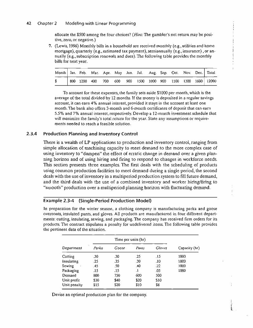
42 Chapter 2 Modeling with Linear Programming
allocate the $500 among the four choices? (Hinl:The gambler's net return may be positive, zero, or negative.)
7. (Lewis, 1996) Monthly bills in a household are received monthly (e.g., utilities and homemortgage), quarterly (e.g., estimated tax payment), semiannually (e.g., insurance) ,or annually (e.g., subscription renewals and dues). The following table provides the monthlybills for next year.
Month Jan. Feb. Mar. Apr. May Jun. luI. Aug. Sep. Oct. Nov. Dec. Total
$ 800 1200 400 700 600 900 1500 1000 900 1100 1300 1600 12000
To account for these expenses, the family sets aside $1000 per month, which is theaverage of the total divided by 12 months. If the money is deposited in a regular savingsaccount, it can earn 4% annual interest, provided it stays in the account at least onemonth. The bank also offers 3-month and 6-month certificates of deposit that can earn5.5% and 7% annual interest, respectively. Develop a 12-month investment schedule thatwill maximize the family's total return for the year. State any assumptions or requirements needed to reach a feasible solution.
2.3.4 Production Planning and Inventory Control
There is a wealth of LP applications to production and inventory control, ranging fromsimple allocation of machining capacity to meet demand to the more complex case ofusing inventory to "dampen" the effect of erratic change in demand over a given planning horizon and of using hiring and firing to respond to changes in workforce needs.This section presents three examples. 'The first deals with the scheduling of productsusing common production facilities to meet demand during a single period, the seconddeals with the use of inventory in a multiperiod production system to fill future demand,and the third deals with the use of a combined inventory and worker hiring/firing to"smooth" production over a multiperiod planning horizon with fluctuating demand.
Example 2.3-4 (Single-Period Production Model)
In preparation for the winter season, a clothing company is manufacturing parka and gooseovercoats, insulated pants, and gloves. All products are manufactured in four different departments: cutting, insulating, sewing, and packaging. The company has received firm orders for itsproducts. TIle contract stipulates a penalty for undelivered items. The following table providesthe pertinent data of the situation.
Time per units (hr)
Department Parka Goose Pants Gloves Capacity (hr)
Cutting .30 .30 .25 .15 1000Insulating .25 .35 .30 .10 1000Sewing .45 .50 .40 .22 1000Packaging .15 .15 .1 .05 1000Demand 800 750 600 500Unit profit $30 $40 $20 $10Unit penalty $15 $20 $10 $8
Devise an optimal production plan for the company.
1
f
;.
s:ll,)
e
ss
1.
:2.3 Selected LP Applications 43
Mathematical Model: The definition of the variables is straightforward. Let
Xl = number of parka jackets
X2 = number of goose jackets
X3 = number of pairs of pants
X4 = number of pairs of gloves
The company is penalized for not meeting demand. 111is means that the objective of the problemis to maximize the net receipts, defined as
Net receipts = Total profit - Total penalty
The total profit is readily expressed as 30xI + 40X2 + 20X3 + 10X4' The total penalty is a function of the shortage quantities (= demand - units supplied of each product). These quantitiescan be determined from the following demand limits:
A demand is not fulfilled if its constraint is satisfied as a strict inequality. For example, if 650parka jackets are produced, then Xl = 650, which leads to a shortage of 800 - 650 = 150 parkajackets. We can express the shortage of any product algebraically by defining a new nonnegativevariable-namely,
Sj = Number of shortage units of product j, j = 1,2,3,4
In this case, the demand constraints can be written as
XI + sl = 800, X2 + S2 = 750, X3 + s3 = 600, X4 + S4 = 500
Xj ;::: 0, Sj ;::: 0, j = 1,2,3,4
We can now compute the shortage penalty as 15s l + 20s2 + lOs3 + 8s4. Thus, the objective function can be written as
To complete the model, the remaining constraints deal with the production capacity restrictions; namely
.30Xl + .30X2 + .25x3 + .15x4 :5 1000 (Cutting)
.25xl + .35x2 + .30X3 + .lOx4 :5 1000 (InSUlating)
.45xl + .50x2 + AOX3 + .22x4 :5 1000 (Sewing)
.15x1 + .15x2 + .10x3 + .05X4 :5 1000 (Packaging)
The complete model thus becomes
44 Chapter 2
subject to
Modeling with Linear Programming
.30XI + .30X2 + .25x3 + .15x4 ::; 1000
.25xl + .35x2 + .30X3 + .10x4 ::; 1000
.45xl + .50x2 + .40X3 + .22x4 ::; 1000
.15xl + .15x2 + .lOx3 + .05X4 :;; 1000
Xl + SI = 800, X2 + S2 = 750, X3 + S3 = 600, X4 + S4 = 500
Xj ~ 0, 5j ~ 0, j = 1, 2, 3, 4
Solution:
The optimum solution is z = $64,625, Xl = 850, X2 = 750, X) = 387.5, X4 = 500, SI = 52 =S4 = 0, s3 = 212.5. The solution satisfies all the demand for both types of jackets and the gloves.A shortage of 213 (rounded up from 212.5) pairs of pants will result in a penalty cost of213 X $10 = $2130.
Example 2.3-5 (Multiple Period Production-Inventory Model)
Acme Manufacturing Company has contracted to deliver horne windows over the next 6 months.The demands for each month are 100,250,190,140,220, and 110 units, respectively. Production costper window varies from month to month depending on the cost of labor, material, and utilities.Acme estimates the production cost per window over the next 6 months to be $50, $45, $55, $48,$52, and $50, respectively. To take advantage of the fluctuations in manufacturing cost, Acme mayelect to produce more than is needed in a given month and hold the excess units for delivery inlater months. This, however, will incur storage costs at the rate of $8 per window per month assessed on end-of-month inventory. Develop a linear program to determine the optimum production schedule.
Mathematical Model: The variables of the problem include the monthly production amountand the end-of-month inventory. For i = 1,2, ... , 6, let
Xi = Number of units produced in month i
1i = Inventory units left at the end of month i
The relationship between these variables and the monthly demand over the six-month horizon isrepresented by the schematic diagram in Figure 2.5. TIle system starts empty, which means that10 = O.
The objective function seeks to minimize the sum of the production and end-of-month inventory costs. Here we have,
Total production cost = 50xI + 45x2 + 55x3 + 48x4 + 52xs + 50X6
Total inventory cost = 8(11 + lz + h + 14 + 15 + I6 )
Thus the objective function is
Minimize z = 50Xl + 45x2 + 55x3 + 48x4 + 52xs + 50X6
+ 8( II + 12 + h + 14 + Is + I6 )
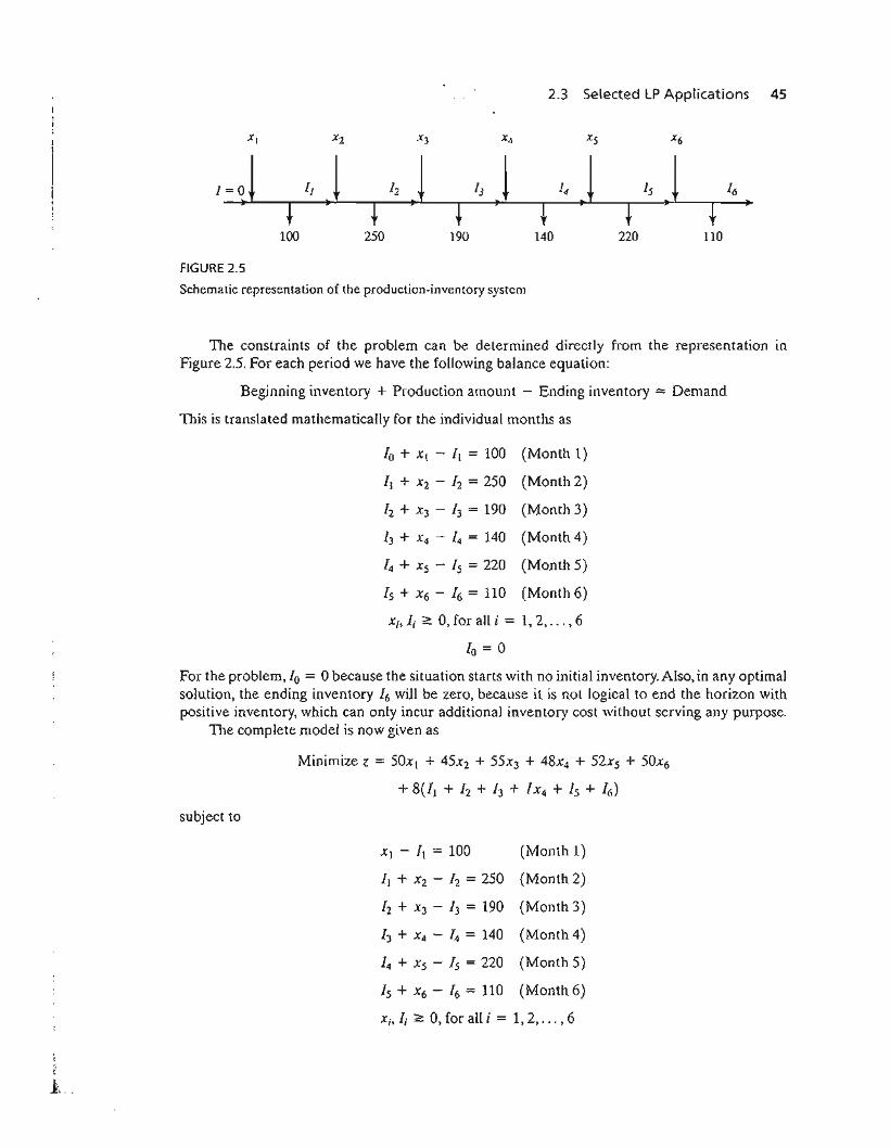
2.3 Selected LP Applications 45
1=0
FIGURE 2.5
100 250 190 140 220 110
Schematic representation of the production-inventory system
The constraints of the problem can be determined directly from the representation inFigure 2.5. For each period we have the following balance equation:
Beginning inventory + Production amount - Ending inventory = Demand
This is translated mathematically for the individual months as
/0 + Xl - /1 = 100 (Month 1)
II + X2 - /2 = 250 (Month 2)
[2 + X3 - /3 = 190 (Month 3)
/3 + X4 - /4 = 140 (Month 4)
14 + X5 - 15 = 220 (Month 5)
15 + X6 - 16 = 110 (Month 6)
Xi, Ii 2:: 0, for all i = 1,2, ... ,6
/0 = 0
For the problem, 10 = 0 because the situation starts with no initial inventory. Also, in any optimalsolution, the ending inventory h will be zero, because it is not logical to end the horizon withpositive inventory, which can only incur additional inventory cost without serving any purpose.
The complete model is now given as
Minimize z = 50Xt + 45x2 + 55x3 + 48x4 + 52x5 + 50X6
+ 8(/1 + h + h + lx4 + /5 + /6)
subject to
XI - /1 = 100 (Month 1)
II + X2 - h = 250 (Month 2)
/2 + X3 - h = 190 (Month 3)
[3 + X4 - 14 = 140 (Month 4)
/4 + Xs - 15 = 220 (Month 5)
Is + X6 - [6 = 110 (Month 6)
Xi' Ii 2:: 0, for all i = 1, 2, ... , 6
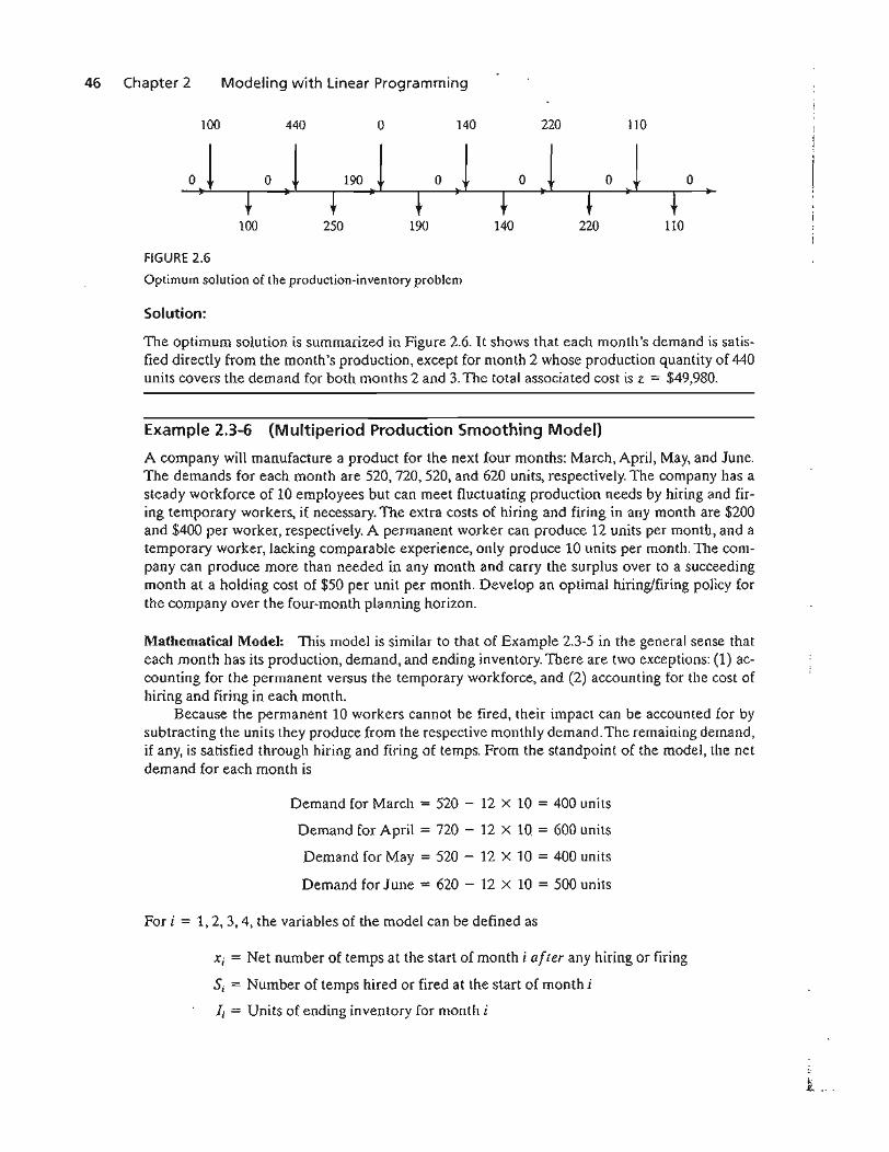
46 Chapter 2 Modeling with Linear Programming
100
o o
440
190
o
o
140
o
220
o
110
o
FIGURE 2.6
100 250 190 140 220 110
Optimum solution of the production.inventory problem
Solution:
The optimum solution is summarized in Figure 2.6. It shows that each month's demand is satisfied directly from the month's production, except for month 2 whose production quantity of 440units covers the demand for both months 2 and 3. The total associated cost is z = $49,980.
Example 2.3-6 (Multiperiod Production Smoothing Model)
A company will manufacture a product for the next four months: March, April, May, and June.The demands for each month are 520, 720, 520, and 620 units, respectively. The company has asteady workforce of 10 employees but can meet fluctuating production needs by hiring and firing temporary workers, if necessary. The extra costs of hiring and firing in any month are $200and $400 per worker, respectively. A permanent worker can produce 12 units per month, and atemporary worker, lacking comparable experience, only produce 10 units per month. TIle company can produce more than needed in any month and carry the surplus over to a succeedingmonth at a holding cost of $50 per unit per month. Develop an optimal hiring/firing policy forthe company over the four-month planning horizon.
Mathematical Model: This model is similar to that of Example 2.3-5 in the general sense thateach month has its production, demand, and ending inventory. There are two exceptions: (1) accounting for the permanent versus the temporary workforce, and (2) accounting for the cost ofhiring and firing in each month.
Because the permanent 10 workers cannot be fired, their impact can be accounted for bysubtracting the units they produce from the respective monthly demand. The remaining demand,if any, is satisfied through hiring and firing of temps. From the standpoint of the model, the netdemand for each month is
Demand for March = 520 - 12 X 10 = 400 units
Demand for April = 720 - 12 X 10 = 600 units
Demand for May = 520 - 12 X 10 = 400 units
Demand for June = 620 - 12 X 10 = 500 units
For i = 1,2,3,4, the variables of the model can be defined as
Xi = Net number of temps at the start of month i after any hiring or firing
Sj = Number of temps hired or fired at the start of month i
Ii = Units of ending inventory for month i
~L ._
2.3 Selected LP Applications 47
The variables Xi and Ii, by definition, must assume nonnegative values. On the other hand, thevariable 5i can be positive when new temps are hired, negative when workers are fired, and zeroif no hiring or firing occurs. As a result, the variable must be unrestricted in sign, This is the firstinstance in this chapter of using an unrestricted variable. As we will see shortly, special substitution is needed to allow the implementation of hiring and firing in the model.
The objective is to minimize the sum of the cost of hiring and firing plus the cost of holdinginventory from one month to the next. The treatment of the inventory cost is similar to the onegiven in Example 2.3-5-namely,
Inventory holding cost = 50( II + h + [3)
(Note that /4 = 0 in the optimum solution.) The cost of hiring and firing is a bit moreinvolved. We know that in any optimum solution, at least 40 temps (= 4~) must behired at the start of March to meet the month's demand. However, rather than treating this situation as a special case, we can let the optimization process take care of it automatically. Thus,given that the costs of hiring and firing a temp are $200 and $400, respectively, we have
(C f I") (NUmber of hired temps )ost o' llnngd f
' . = 200 at the start ofan mng
March, April, May, and June
(
Number of fired temps )+ 400 at the start of
March, April, May, and June
To translate this equation mathematically, we will need to develop the constraints first.The constraints of the model deal with inventory and hiring and firing. First we develop the
inventory constraints. Defining X, as the number of temps available in month i and given that theproductivity of a temp is 10 units per month, the number of units produced in the same month islOXi' Thus the inventory constraints are
lOx! = 400 + 11 (March)
I, + lOx2 = 600 + 12 (April)
12 + lOx3 = 400 + /3 (May)
13 + 10x4 = 500 (June)
Next, we develop the constraints dealing with hiring and firing. First, note that the temp workforce starts with XI workers at the beginning of March. At the start of April, XI will be adjusted(up or down) by 52 to generate X2' The same idea applies to x3 and X4' These observations lead tothe following equations
XI = 5\
X2 = Xl + 52
x) = X2 + 53
48 Chapter 2 Modeling with Linear Programming
X4 = X3 + 54
51> 52, 53, 54 unrestricted in sign
The variables 51> 5z, 53, and 54 represent hiring when they are strictly positive and firingwhen they are strictly negative. However, this "qualitative" information cannot be used in amathematical expression. Instead, we use the following substitution:
5j = Si - 5;, where 5j, 5; ~ 0
The unrestricted variable Sj is now the difference between two nonnegative variables 5j and Sf.We can think of 5i as the number of temps hired and 5; as the number of temps fired. For example, if Sj = 5 and 5t = 0 then 5i = S - 0 = +S, which represents hiring. If 5i = 0 and5t = 7 then Sj = 0 - 7 = -7, which represents firing. In the first case, the corresponding costof hiring is 2005i = 200 X S = $1000 and in the second case the corresponding cost of firing is4005; = 400 X 7 = $2800. This idea is the basis for the development of the objective function.
First we need to address an important point: What if both 5j and 5t are positive? TIle answer is that this cannot happen because it implies that the solution calls for both hiring and firingin the same month. Interestingly, the theory of linear programming (see Chapter 7) tells us that5i and 5t can never be positive simultaneously, a result that confirms intuition.
We can now write the cost of hiring and firing as follows:
Cost of hiring = 200{51 + 52 + 5"3 + 5:1)
Cost of firing = 400(51' + 51 + 51 + 5t)
The complete model is
Minimize z = 50(11 + lz + I} + 14 ) + 200(51 + 52 + 5"3 + 5;)
+ 400(5j + 5r + 5r + S:1')
subject to
lOx 1 = 400 + 11
1, + 10xz = 600 + 12
lz + lOx3 = 400 + 13
h + lOx4 = SOO
Xl = 51 - 51'
Xz = X I + 52 - 5r
X3 = Xz + 5:; - 5j
X4 = X3 + 54 - 5t
5j, 5j, 5;,5!, 5"3, 5j, 5;, 5t ~ 0
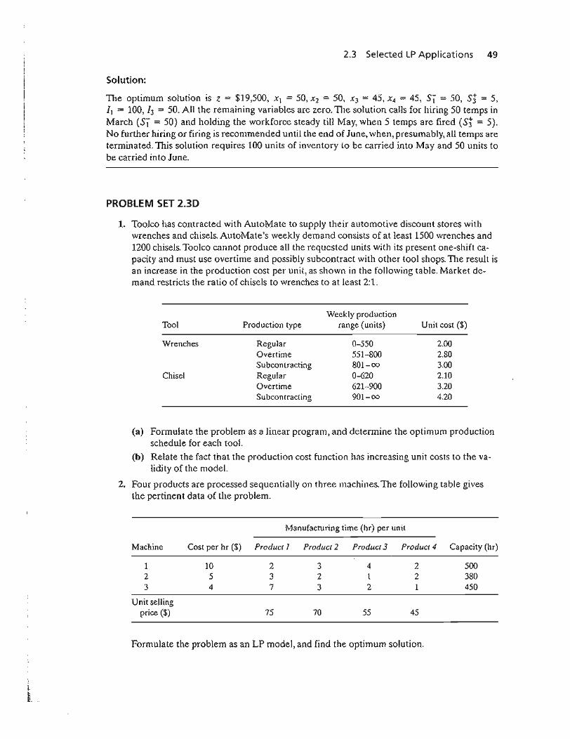
2.3 Selected LP Applications 49
Solution:
The optimum solution is z = $19,500, Xl = 50, Xl = 50, -'3 = 45, X4 = 45, 5\ = 50, Sr = 5,II = 100, /3 = 50. All the remaining variables are zero. TIle solution calls for hiring 50 temps inMarch (51 = 50) and holding the workforce steady till May, when 5 temps are fired (5j = 5).No further hiring or firing is recommended until the end of June, when, presumably, all temps areterminated. This solution requires 100 units of inventory to be carried into May and 50 units tobe carried into June.
PROBLEM SET 2.30
1. Tooleo has contracted with AutoMate to supply their automotive discount stores withwrenches and chisels. AutoMate's weekly demand consists of at least 1500 wrenches and1200 chisels. Tooleo cannot produce all the requested units with its present one-shift capacity and must use overtime and possibly subcontract with other tool shops. The result isan increase in the production cost per unit, as shown in the following table. Market demand restricts the ratio of chisels to wrenches to at least 2:1.
Weekly productionTool Production type range (units) Unit cost ($)
Wrenches Regular 0-550 2.00Overtime 551-800 2.80Subcontracting 801-00 3.00
Chisel Regular 0-620 2.10Overtime 621-900 3.20Subcontracting 901-00 4.20
(a) Formulate the problem as a linear program, and determine the optimum productionschedule for each tool.
(b) Relate the fact that the production cost function has increasing unit costs to the validi ty of the modeL
2. Four products are processed sequentially on three machines. The following table givesthe pertinent data of the problem.
Manufacturing time (hr) per unit
Machine Cost per hr ($) Productl Product 2 Product 3 Product 4 Capacity (hr)
1 10 2 3 4 2 5002 5 3 2 1 2 3803 4 7 3 2 1 450
Unit sellingprice ($) 75 70 55 45
Formulate the problem as an LP model, and find the optimum solution.
2.3 Selected LP Applications 51
TIle production rates in units per hour are 1.25 and 1 for products A and B, respectively. All demand must be met. However, demand for a later month may be filled fromthe production in an earlier one. For any carryover from one month to the next, holdingcosts of $.90 and $.75 per unit per month are charged for products A and B, respectively.The unit production costs for the two products are $30 and $28 for A and B, respectively.Determine the optimum production schedule for the two products.
*7. The manufacturing process of a product consists of two successive operations, I and II. Thefollowing table provides the pertinent data over the months of June, July, and August:
,,. ,,
Finished product demand (units)Capacity of operation I (hr)Capacity of operation II (hr)
June
500800
1000
July
450700850
August
600550700
Producing a unit of the product takes .6 hour on operation I plus .8 hour on operationII. Overproduction of either the semifinished product (operation I) or the finishedproduct (operation II) in any month is allowed for use in a later month. The corresponding holding costs are $.20 and $.40 per unit per month. The production cost variesby operation and by month. For operation 1, the unit production cost is $10, $12, and$11 for June, July, and August. For operation 2, the corresponding unit production costis $15, $18, and $16. Determine the optimal production schedule for the two operationsover the 3-month horizon.
8. Two products are manufactured sequentially on two machines. The time available oneach machine is 8 hours per day and may be increased by up to 4 hours of overtime, ifnecessary, at an additional cost of $100 per hour. The table below gives the productionrate on the two machines as well as the price per unit of the two products. Determine theoptimum production schedule and the recommended use of overtime, if any.
Production rate (unils/hr)
Machine 1Machine 2Price per unit ($)
Product 1
58
110
Product 2
54
118
2.3.5 Blending and Refining
A number of LP applications deal with blending different input materials to produceproducts that meet certain specifications while minimizing cost or maximizing profit.The input materials could be ores, metal scraps, chemicals, or crude oils and the outputproducts could be metal ingots, paints, or gasoline of various grades. This section presents a (simplified) model for oil refining. The process starts with distilling crude oil toproduce intermediate gasoline stocks and then blending these stocks to produce finalgasolines. The final products must satisfy certain quality specifications (such as octanerating). In addition, distillation capacities and demand limits can directly affect thelevel of production of the different grades of gasoline. One goal of the modeLis determine the optimal mix of final products that will maximize an appropriate profit function. In some cases, the goal may be to minimize a cost function.
Example 2.3-7 (Crude Oil Refining and Gasoline Blending)
Shale Oil, located on the island of Aruba, has a capacity of 1,500,000 bbl of crude oil per day. Thefinal products from the refinery include three types of unleaded gasoline with different octanenumbers (ON): regular with ON = 87, premium with ON = 89, and super with ON = 92. Therefining process encompasses three stages: (1) a distillation tower that produces feedstock(ON = 82) at the rate of .2 bbl per bbl of crude oil, (2) a cracker unit that produces gasolinestock (ON = 98) by using a portion of the feedstock produced from the distillation tower at therate of .5 bbl per bbl of feedstock, and (3) a blender unit that blends the gasoline stock from thecracker unit and the feedstock from the distillation tower. The company estimates the net profitper barrel of the three types of gasoline to be $6.70, $7.20, and $8.10, respectively. The input capacity of the cracker unit is 200,000 barrels of feedstock a day. TIle demand limits for regular,premium, and super gasoline are 50,000,30,000, and 40,000 barrels per day. Develop a model fordetermining the optimum production schedule for the refinery.
")j.,I,i,
IIIII
S2 Chapter 2 Modeling with Linear Programming
Mathematical Model: Figure 2.7 summarizes the elements of the model. TIle variables can bedefined in terms of two input streams to the blender (feedstock and cracker gasoline) and thethree final products. Let
Xij = bbl/day of input stream i used to blend final product j, i = 1,2; j = 1,2,3
Using this definition, we have
Daily production of regular gasoline = XII + X21 bbl/dayDaily production of premium gasoline = X12 + X22 bbl/dayDaily production of super gasoline = xn + X23 bbllday
(Daily output ) = (DailY Production) + (DailY Production)
of blender unit of regular gas of premium gas
+ (DailY Production)of super gas
= (Xli + X21) + (X12 + X22) + (XJ3 + x23)bbl/day
1:1
Xll + X12 + XlJ --ON =82
5:1 2:1 Blender --Crude
Distillation Crackerx21 + xn + x23
ON =82 ON =98 ~
Feed-stock
XII + x21, ON = 87
Xl3 + x23' ON = 92
FIGURE 2.7
Product flow in the refinery problem
i1
2.3 Selected LP Applicatio'ns . 53
(Daily feedstoCk)
bl d= XIl + Xl2 + Xn bbl/day
to en er
(Daily cracker unit)
f d bl d= X2l + Xn + x23 bbl/day
ee to en er
(Daily feedstoCk)
k= 2(X21 + X22 + X23)bbl/day
to crac er
(Daily crude oil used)
"I f" = 5(Xll + X12 + XI3) + 10(X21 + X22 + x23)bbIldayIn t le re mery
The objective of the model is to maximize the total profit resulting from the sale of all threegrades of gasoline. From the definitions given above, we get
Maximize z = 6.70(x]] + x2d + 7.20(XI2 + X22) + 8.1O(X13 + X23)
The constraints of the problem are developed as follows:
1. Daily crude oil supply does /lot exceed 1,500,000 bbl/day:
5(xl1 + XI2 + xn) + 10(X21 + X22 + X23) ::5 1,500,000
2. Cracker unit input capacity does not exceed 200,000 bbl/day:
2(X21 + X22 + X23) ::5 200,000
3. Daily demand for regular does not exceed 50,000 bbl:
Xl I + x21 ::5 50,000
4. Daily demand for premium does not exceed 30,000:
XI2 + X22 ::5 30,000
5. Daily demand for super does not exceed 40,000 bbl:
Xu + x23 ::5 40,000
6. Octane number (ON) for regular is at least 87:
TIle octane number of a gasoline product is the weighted average of the octane numbers ofthe input streams used in the blending process and can be computed as
(Average ON Of)regular gasoline =
Feedstock ON X feedstock bbl/day + Cracker unit ON X Cracker unit bbl/day
Total bbl/day of regular gasoline
82xl1 + 98x21=
Thus, octane number constraint for regular gasoline becomes
82xlI + 98x21---:...::...--.....::..:..;;::87XII + X2I
54 Chapter 2 Modeling with Linear Programming
The constraint is linearized as
82xll + 98x21 2:: 87(Xll + X2l)
7. Octane number (ON) for premium is at least 89:
82x12 + 98x22_--..::.=:._--= 2:: 89X12 + X22
which is linearized as
82xl2 + 98x22 2:: 89(xl2 + X22)
8. Octane number (ON) for super is at least 92:
82x13 + 98x23_--..::.=:._--= 2:: 92X13 + X23
or
The complete model is thus summarized as
Maximize z = 6.70(xlI + x2d + 7.20(xl2 + X22) + 8.10(xl3 + X23)
subject to
5(xll + XI2 + X13) + 1O(X2I + X22 + X23) :5 1,500,000
2(Xll + Xl2 + Xl3) :5 200,000
Xli + X2I :5 50,000
XI2 + Xn :5 30,000
X13 + X23 :5 40,000
82xll + 98x2I 2:: 87(xu + x2d
82x12 + 98x22 2:: 89(x12 + X22)
82x13 + 98x23 2:: 92(X13 + Xl3)
The last three constraints can be simplified to produce a constant right-hand side.
Solution:
The optimum solution (using file amplEx2.3-7.txt) is z = 1,482,000, Xu = 20,625, Xli == 9375,XI2 =' 16,875, X22 = 13,125, Xl3 = 15,000, X23 = 25,000. This translates to
Daily profit = $1,482,000
Daily amount of regular gasoline = XII + XlI = 20,625 + 9375 = 30,000 bbl/day
Daily amount of premium gasoline = Xu + xn = 16,875 + 13,125 = 30,000 bbVday
Daily amount of regular gasoline = XI3 + X23 = 15,000 + 25,000 = 40,000 bbVday
The solution shows that regular gasoline production is 20,000 bbVday short of satisfying themaximum demand. The demand for the remaining two grades is satisfied.
75,
the
2.3 Selected LP Applications 55
PROBLEM SET 2.3E
1. Hi-V produces three types of canned juice drinks, A, B, and C, using fresh strawberries,grapes, and apples. TIle daily supply is limited to 200 tons of strawberries, 100 tons ofgrapes, and 150 tons of apples. The cost per ton of strawberries, grapes, and apples is $200,$100, and $90, respectively. Each ton makes 1500 Ib of strawberry juice, 1200 Ib of grapejuice, and 1000 Ib of apple juice. Drink A is a 1:1 mix of strawberry and apple juice. Drink Bis 1:1:2 mix of strawberry, grape, and apple juice. Drink C is a 2:3 mix of grape and applejuice. All drinks are canned in 16-oz (lib) cans. The price per can is $1.15, $1.25, and $1.20for drinks A, B, and C. Determine the optimal production mix of the three drinks.
*2. A hardware store packages handyman bags of screws, bolts, nuts, and washers. Screws comein 100-lb boxes and cost $110 each, bolts come in 1oo-lb boxes and cost $150 each, nuts comein 80-lb boxes and cost $70 each, and washers come in 30-lb boxes and cost $20 each. Thehandyman package weighs at least lib and must include, by weight, at least 10% screws and25% bolts, and at most 15% nuts and 10% washers. To balance the package, the number ofbolts cannot exceed the number of nuts or the number of washers. A bolt weighs 10 times asmuch as a nut and 50 times as much as a washer. Determine the optimal mix of the package.
3. All-Natural Coop makes three breakfast cereals, A, B, and C, from four ingredients:rolled oats, raisins, shredded coconuts, and slivered almonds. The daily availabilities of theingredients are 5 tons, 2 tons, 1 ton, and 1 ton, respectively. The corresponding costs perton are $100, $120, $110, and $200. Cereal A is a 50:5:2 mix of oats, raisins, and almond.Cereal B is a 60:2:3 mix of oats, coconut, and almond. Cereal C is a 60:3:4:2 mix of oats,raisins, coconut, and almond. The cereals are produced in jumbo 5-lb sizes. All-Naturalsells A, B, and Cat $2, $2.50, and $3.00 per box, respectively. The minimum daily demandfor cereals A, B, and Cis 500,600, and 500 boxes. Determine the optimal production mixof the cereals and the associated amounts of ingredients.
4. A refinery manufactures two grades of jet fuel, f1 and Fl, by blending four types of gasoline, A, B, C, and D. Fuel F1 uses gasolines A, B, C, and D in the ratio 1:1:2:4, and fuel Fluses the ratio 2:2:1:3. The supply limits for A, B, C, and Dare 1000, 1200,900, and 1500bbllday, respectively. The costs per bbl for gasolines A, B, C, and Dare $120, $90, $100, and$150, respectively. Fuels F1 and Fl sell for $200 and $250 per bbi.The minimum demandfor F1 and Fl is 200 and 400 bbUday. Determine the optimal production mix for F1 and n.
5. An oil company distills two types of crude oil, A and B, to produce regular and premiumgasoline and jet fuel. There are limits on the daily availability of crude oil and the minimumdemand for the final products. If the production is not sufficient to cover demand, the shortage must be made up from outside sources at a penalty. Surplus production will not be soldimmediately and will incur storage cost. The following table provides the data of the situation:
Fraction yield per bbl
Crude Regular Premium Jet Price/bbl ($) bbl/day
Crude A .20 .1 .25 30 2500Crude B .25 .3 .10 40 3000Demand (bbllday) 500 700 400Revenue ($/bbl) 50 70 120Storage cost for surplus
production ($ibbl) 2 3 4Penalty for unfilled
demand ($/bbl) 10 15 20
Determine the optimal product mix for the refinery.
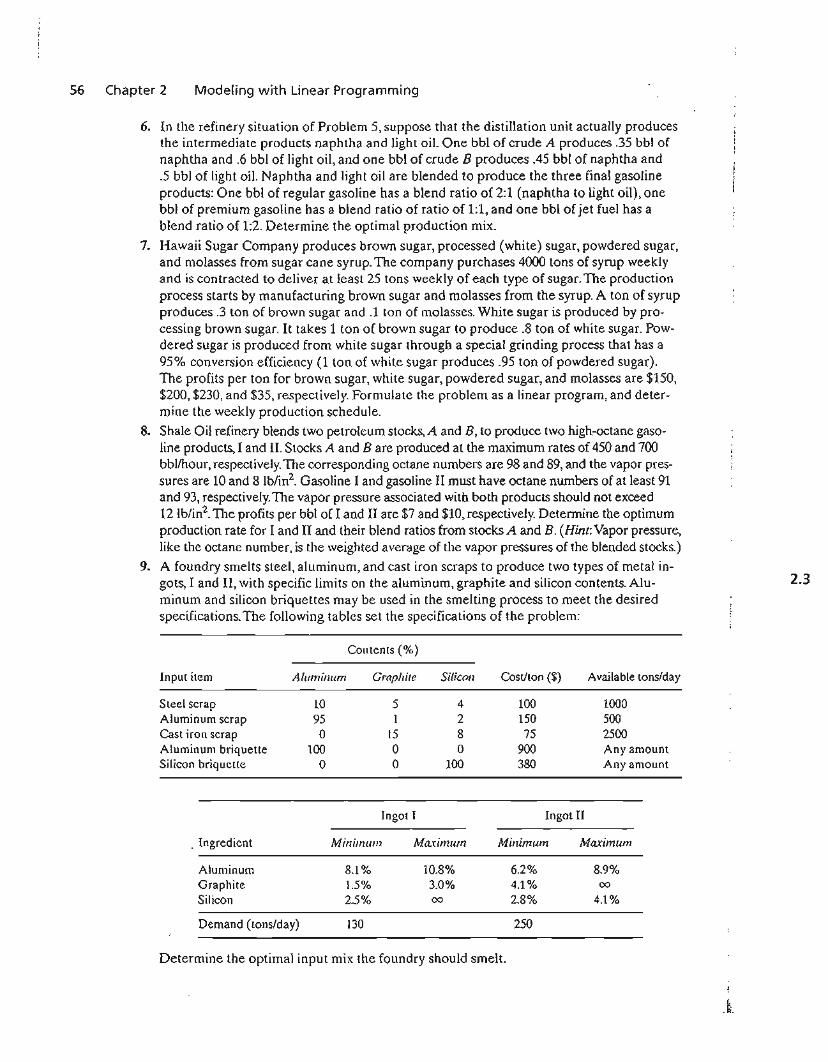
56 Chapter 2 Modeling with Linear Programming
6. In the refinery situation of Problem 5, suppose that the distillation unit actually producesthe intermediate products naphtha and light oil. One bbl of crude A produces .35 bbl ofnaphtha and .6 bbl of light oil, and one bbl of crude B produces .45 bbl of naphtha and.5 bbl of light oil. Naphtha and light oil are blended to produce the three final gasolineproducts: One bbl of regular gasoline has a blend ratio of 2:1 (naphtha to light oil), onebbl of premium gasoline has a blend ratio of ratio of 1:1, and one bbl of jet fuel has ablend ratio of 1:2. Determine the optimal production mix.
7. Hawaii Sugar Company produces brown sugar, processed (white) sugar, powdered sugar,and molasses from sugar cane syrup. The company purchases 4000 tons of syrup weeklyand is contracted to deliver at least 25 tons weekly of each type of sugar. The productionprocess starts by manufacturing brown sugar and molasses from the syrup. A ton of syrupproduces .3 ton of brown sugar and .1 ton of molasses. White sugar is produced by processing brown sugar. It takes 1 ton of brown sugar to produce .8 ton of white sugar. Powdered sugar is produced from white sugar through a special grinding process that has a95% conversion efficiency (1 ton of white sugar produces .95 ton of powdered sugar).The profits per ton for brown sugar, white sugar, powdered sugar, and molasses are $150,$200, $230, and $35, respectively. Formulate the problem as a linear program, and determine the weekly production schedule.
8. Shale Oil refinery blends two petroleum stocks,A and B, to produce two high-octane gasoline products, I and II. Stocks A and B are produced at the maximum rates of 450 and 700bbUhour, respectively. The corresponding octane numbers are 98 and 89, and the vapor pressures are 10 and 8 Ib/in2. Gasoline I and gasoline II must have octane numbers of at least 91and 93, respectively. The vapor pressure associated with both products should not exceed12 Ib/in2. The profits per bbl of I and II are $7 and $10, respectively. Determine the optimumproduction rate for I and II and their blend ratios from stocks A and B. (Hint: Vapor pressure,like the octane number, is the weighted average of the vapor pressures of the blended stocks.)
9. A foundry smelts steel, aluminum, and cast iron scraps to produce two types of metal ingots, I and II, with specific limits on the aluminum, graphite and silicon contents. Aluminum and silicon briquettes may be used in the smelting process to meet the desiredspecifications. The following tables set the specifications of the problem:
Contents (%)
Input item Aluminum Graphite Silicon Cost/ton ($) Available tons/day
Steel scrap 10 5 4 100 1000Aluminum scrap 95 1 2 150 500Cast iron scrap 0 15 8 75 2500Aluminum briquette 100 0 0 900 Any amountSilicon briquette 0 0 100 380 Any amount
2.3
Ingot I Ingot II
. Ingredient
AluminumGraphiteSilicon
Demand (tons/day)
Minimum
8.1%1.5%2.5%
130
Maximum
10.8%3.0%00
Minimum
6.2%4.1%2.8%
250
Maximum
8.9%00
4.1%
Determine the optimal input mix the foundry should smelt.
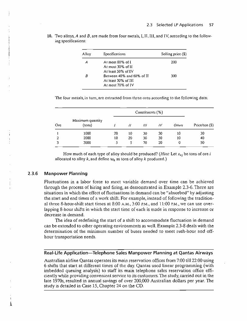
2.3 Selected LP Applications 57
10. Two alloys, A and B, are made from fOUf metals, I, II, III, and IV, according to the following specifications:
Alloy
A
B
Specifications
At most 80% of IAt most 30% of IIAt least 50% of IVBetween 40% and 60% of IIAt least 30% of IIIAt most 70% of IV
Selling price ($)
200
300
The fOUf metals, in turn, are extracted from three ores according to the following data:
Constituents (%)
Maximum quantityOre (tons) I If 1lI IV Others Price/ton ($)
1 1000 20 ]0 30 30 10 302 2000 10 20 30 30 10 403 3000 5 5 70 20 0 50
How much of each type of alloy should be produced? (Hint: Let Xkj be tons of are iallocated to alloy k, and define Wk as tons of alloy k produced.)
2.3.6 Manpower Planning
Fluctuations in a labor force to meet variable demand over time can be achievedthrough the process of hiring and firing, as demonstrated in Example 2.3-6. There aresituations in which the effect of fluctuations in demand can be "absorbed" by adjustingthe start and end times of a work shift. For example, instead of following the traditional three 8-hour-shift start times at 8:00 A.M., 3:00 P.M., and 11:00 P.M., we can use overlapping 8-hour shifts in which the start time of each is made in response to increase ordecrease in demand.
TIle idea of redefining the start of a shift to accommodate fluctuation in demandcan be extended to other operating environments as well. Example 2.3-8 deals with thedetermination of the minimum number of buses needed to meet rush-hour and offhour transportation needs.
Real-Life Application-Telephone Sales Manpower Planning at Qantas Airways
Australian airline Qantas operates its main reservation offices from 7:00 till 22:00 using6 shifts that start at different times of the day. Qantas used linear programming (withimbedded queuing analysis) to staff its main telephone sales reservation office efficiently while providing convenient service to its customers. The study, carried aut in thelate 1970s, resulted in annual savings of over 200,000 Australian dollars per year. Thestudy is detailed in Case 15, Chapter 24 on the CD.
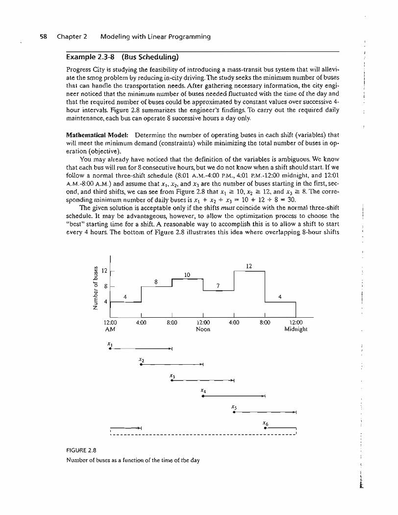
58 Chapter 2 Modeling with linear Programming
Example 2.3-8 (Bus Scheduling)
Progress City is studying the feasibility of introducing a mass-transit bus system that will alleviate the smog problem by reducing in-city driving. The study seeks the minimum number of busesthat can handle the transportation needs. After gathering necessary information, the city engineer noticed that the minimum number of buses needed fluctuated with the time of the day andthat the required number of buses could be approximated by constant values over successive 4hour intervals. Figure 2.8 summarizes the engineer's findings. To carry out the required dailymaintenance, each bus can operate 8 successive hours a day only.
Mathematical Model: Determine the number of operating buses in each shift (variables) thatwill meet the minimum demand (constraints) while minimizing the total number of buses in operation (objective).
You may already have noticed that the definition of the variables is ambiguous. We knowthat each bus will run for 8 consecutive hours, but we do not know when a shift should start. If wefollow a normal three-shift schedule (8:01 A.M.-4:00 P.M., 4:01 p.M.-12:00 midnight, and 12:01A.M.-8:00 A.M.) and assume that x(, X2, and X3 are the number of buses starting in the first, second, and third shifts, we can see from Figure 2.8 that Xl ~ 10, x2 ::=: 12, and X3 ::=: 8. The corresponding minimum number of daily buses is Xl + X2 + X3 = 10 + 12 + 8 = 30.
The given solution is acceptable only if the shifts must coincide with the norma) three-shiftschedule. It may be advantageous, however, to allow the optimization process to choose the"best" starting time for a shift. A reasonable way to accomplish this is to allow a shift to startevery 4 hours. The bottom of Figure 2.8 illustrates this idea where overlapping 8-hour shifts
V> 12oJ 12 l-V>
10::l.0....
88 I I 70 f--.... IoJ
.0 4 4E 4::l
IzI I I I I
12:00 4:00 8:00 12:00 4:00 8:00 12:00AM Noon Midnight
XI• • I
x2• -I
x3• • I
x4• • I
Xs• • I
X6-----+-I.I • I
~------------~---~--------------------------- I
FIGURE 2.8
Number of buses as a function of the time of the day
2.3 Selected LP Applications 59
may start at 12:01 A.M., 4:01 A.M., 8:01 A.M., 12:01 P.M., 4:01 P.M., and 8:01 P.M.lllUS, the variables may be defined as
XI = number of buses starting at 12: 01 A.M.
X2 = number of buses starting at 4:01 A.M.
X3 = number of buses starting at 8:01 A.M.
X4 = number of buses starting at 12:01 P.M.
Xs = number of buses starting at 4:01 P.M.
X6 = number of buses starting at 8:01 P.M.
We can see from Figure 2.8 that because of the overlapping of the shifts, the number of buses forthe successive 4-hour periods is given as
Time period
12:01 A.M. - 4:00 A.M.
4:01 A.M. - 8:00 A.M.
8:01 A.M. -12:00 noon12:01 P.M. - 4:00 P.M.
4:01 P.M. - 8:00 P.M.
8:01 A.M. -12:00 A.M.
Number of buses in operation
X\ + X6
XI + X2
X2 + X3
XJ + X4
X4 + XsX5 + X6
The complete model is thus written as
Minimize z = X\ + X2 + X3 + X4 + Xs + X6
subject to
X\ + X6 2:: 4 (12:01 A.M.-4:00 A.M.)
X\ + X2 2:: 8 (4:01 A.M.-8:00 A.M.)
X2 + X3 2:: 10 (8:01 A.M.-12:00 noon)
X3 + X4 2:: 7 (12:01 r.M.-4:00 P.M.)
X4 + X5 2:: 12 (4:01 p.M.-8:00 P.M.)
Xs + x6?; 4 (8:01 p.M.-12:00 P.M.)
Xj 2:: O,j = 1,2, ... ,6
Solution:
The optimal solution calls for using 26 buses to satisfy the demand with x. = 4 buses to start at12:01 A.M., X2 = 10 at 4:01 A.M., X4 = 8 at 12:01 P.M., and Xs = 4 at 4:01 P.M.
PROBLEM SET 2.3F
*1. In the bus scheduling example suppose that buses can run either 8- or 12-hour shi-fts. If abus runs for 12 hours, the driver must be paid for the extra hours at 150% of the regularhourly pay. Do you recommend the use of 12-hour shifts?
60 Chapter 2 Modeling with Linear Programming
2. A hospital employs volunteers to staff the reception desk between 8:00 A.M. and 10:00 P.M.
Each volunteer works three consecutive hours except for those starting at 8:00 P.M. whowork for two hours only. The minimum need for volunteers is approximated by a stepfunction over 2-hour intervals starting at 8:00 A.M. as 4, 6, 8, 6, 4, 6, 8. Because most volunteers are retired individuals, they are willing to offer their services at any hour of the day(8:00 A.M. to 10:00 P.M.). However, because of the large number of charities competing fortheir service, the number needed must be kept as low as possible. Determine an optimalschedule for the start time of the volunteers
3. In Problem 2, suppose that no volunteers will start at noon or 6:00 P.M. to allow for lunchand dinner. Determine the optimal schedule.
4. In an LTL (less-than-truckload) trucking company, terminal docks include casual workers who are hired temporarily to account for peak loads. At the Omaha, Nebraska, dock,the minimum demand for casual workers during the seven days of the week (starting onMonday) is 20, 14, 10, 15, 18, 10, 12 workers. Each worker is contracted to work five consecutive days. Determine an optimal weekly hiring practice of casual workers for thecompany.
*5. On most university campuses students are contracted by academic departments to do errands, such as answering the phone and typing. The need for such service fluctuates during work hours (8:00 A.M. to 5:00 P.M.). In the IE department, the minimum number ofstudents needed is 2 between 8:00 A.M. and 10:00 A.M.,3 between 10:01 A.M. and 11:00A.M.,4 between 11:01 A.M. and 1:00 P.M., and 3 between 1:01 P.M. and 5:00 P.M. Each student is allotted 3 consecutive hours (except for those starting at 3:01, who work for2 hours and those who start at 4:01, who work for one hour). Because of their flexibleschedule, students can usually report to work at any hour during the work day, exceptthat no student wants to start working at lunch time (12:00 noon). Determine the minimum number of students the IE department should employ and specify the time of theday at which they should report to work.
6. A large department store operates 7 days a week. The manager estimates that the minimum number of salespersons required to provide prompt service is 12 for Monday, 18 forTuesday, 20 for Wednesday, 28 for Thursday, 32 for Friday, and 40 for each of Saturday'and Sunday. Each salesperson works 5 days a week, with the two consecutive off-daysstaggered throughout the week. For example, if 10 salespersons start on Monday, two cantake their off-days on Tuesday and Wednesday, five on Wednesday and Thursday, andthree on Saturday and Sunday. How many salespersons should be contracted and howshould their off-days be allocated?
2.3.7 Additional Applications
The preceding sections have demonstrated the application of LP to six representativeareas. The fact is that LP enjoys diverse applications in an enormous number of areas.The problems at the end of this section demonstrate some of these areas, ranging fromagriculture to military applications. This section also presents an interesting applicationthat deals with cutting standard stocks of paper rolls to sizes specified by customers.
Example 2.3-9 (Trim Loss or Stock Slitting)
The Pacific Paper Company produces paper rolls with a standard width of 20 feet each. Specialcustomer orders with different widths are produced by slitting the standard rolls. Typical orders(which may vary daily) are summarized in the following table:
I,I·
1_ ..
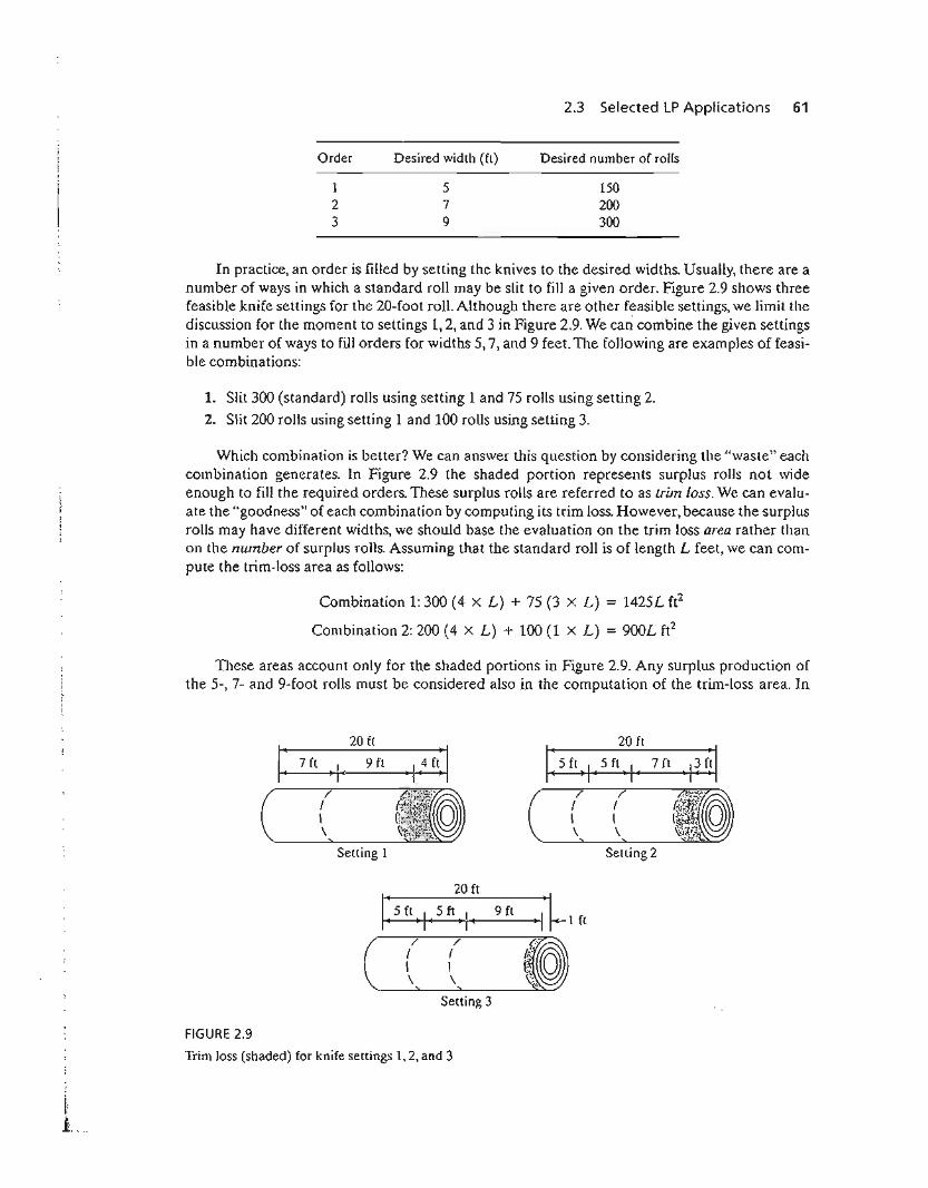
2.3 Selected LP Applications 61
Order Desired width (ft) Desired number of rolls
123
579
150200300
In practice, an order is filled by setting the knives to the desired widths. Usually, there are anumber of ways in which a standard roll may be slit to fill a given order. Figure 2.9 shows threefeasible knife settings for the 20-foot roll. Although there are other feasible settings, we limit thediscussion fOT the moment to settings 1,2, and 3 in Figure 2.9. We can combine the given settingsin a number of ways to fill orders for widths 5,7, and 9 feet. The following are examples of feasible combinations:
1. Slit 300 (standard) rolls using setting 1 and 75 rolls using setting 2.
2. Slit 200 rolls using setting 1 and 100 rolls using setting 3.
Which combination is better? We can answer this question by considering the "waste" eachcombination generates. In Figure 2.9 the shaded portion represents surplus rolls not wideenough to fill the required orders. These surplus rolls are referred to as trim loss. We can evaluate the "goodness" of each combination by computing its trim loss. However, because the surplusrolls may have different widths, we should base the evaluation on the trim loss area rather thanon the number of surplus rolls. Assuming that the standard roll is of length L feet, we can compute the trim-loss area as follows:
Combination 1: 300 (4 X L) + 75 (3 X L) = 1425L ff
Combination 2: 200 (4 X L) + 100 (1 X L) = 900L ft2
111ese areas account only for the shaded portions in Figure 2.9. Any surplus production ofthe 5-, 7- and 9-foot rolls must be considered also in the computation of the trim-loss area. In
I" I"I I\ I\ \
20 ft~-,-7-ft-
20 ft
I"(
\\
I: 7ft '1-0( 9ft
Setting 1 Setting 2
20 ft
~.9ftI" I"
( (I \\ \
Setting 3
FIGURE 2.9
Trim loss (shaded) (or knife settings 1.2. and 3
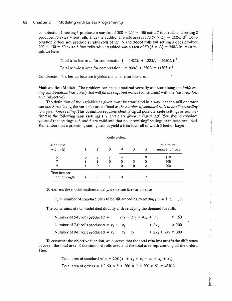
62 Chapter 2 Modeling with Linear Programming
combination 1, setting 1 produces a surplus of 300 - 200 = 100 extra 7-foot rolls and setting 2produces 75 extra 7-foot rolls. Thus the additional waste area is 175 (7 x L) = 1225L ft2. Combination 2 does not produce surplus rolls of the 7- and 9-foot rolls but setting 3 does produce200 - 150 = 50 extra 5-foot rolls, with an added waste area of 50 (5 x L) = 250L ft2
• As a result we have
Total trim-loss area for combination 1 = 1425L + 1225L = 2650L ft2
Total trim-loss area for combination 2 = 900L + 250L = 1150L ft2
Combination 2 is better, because it yields a smaller trim-loss area.
Mathematical Model: The problem can be summarized verbally as determining the knife-setting combinations (variables) that will fill the required orders (constraints) with the least trim-lossarea (objective).
The definition of the variables as given must be translated in a way that the mill operatorcan use. Specifically, the variables are defined as the number ofstandard rolls to be slit accordingto a given knife setting. 111is definition requires identifying all possible knife settings as summarized in the following table (settings 1,2, and 3 are given in Figure 2.9). You should convinceyourself that settings 4,5, and 6 are valid and that no "promising" settings have been excluded.Remember that a promising setting cannot yield a trim-loss roll of width 5 feet or larger.
Knife setting
Required Minimumwidth (ft) I 2 3 4 5 6 number of rolls
5 0 2 2 4 1 0 1507 1 1 0 0 2 0 2009 1 0 1 0 0 2 300
Trim loss perfoot of length 4 3 0 2
To express the model mathematically, we define the variables as
Xj = number of standard rolls to be slit according to setting j, j = 1,2, ... ,6
The constraints of the model deal directly with satisfying the demand for rolls.
Number of 5-ft rolls produced =
Number of 7-ft rolls produced = Xl + X2
~ 150
~ 200
Number of 9-ft rolls produced = Xl
To construct the objective function, we observe that the total "trim loss area is the differencebetween the total area of the standard rolls used and the total area representing all the orders.Thus
Total area of standard rolls = 20L(x) + X2 + X3 + X4 + Xs + X6)
Total area of orders = L(150 x 5 + 200 x 7 + 300 X 9) = 4850L
;j
f1_
2.3 Selected LP Applications 63
The objective function then becomes
Minimize z = 20L(XI + X2 + X3 + X4 + X5 + X6) - 4850L
Because the length L of the standard roll is a constant, the objective function equivalentlyreduces to
Minimize Z = Xl + X2 + X3 + X4 + Xs + X6
The model may thus be written as
Minimize z = Xl + X2 + X3 + X4 + Xs + X6
subject to
Solution:
2X2 + 2X3 + 4X4 + Xs
Xl + X2 + 2X5
Xl + x) + 2X6
Xj;=: O,j = 1,2, ... ,6
;=: 150 (5-ft rolls)
;=: 200 (7-ft rolls)
;=: 300 (9-ft rolls)
,{.I
--l __
The optimum solution calls for cutting 12.5 standard rolls according to setting 4, 100 according tosetting 5, and 150 according to setting 6. TIle solution is not impIementable because X4 is noninteger. We can either use an integer algorithm to solve the problem (see Chapter 9) or round X4
conservatively to 13 rolls.
Remarks. TIle trim-loss model as presented here assumes that all the feasible knife settings canbe determined in advance. This task may be difficult for large problems, and viable feasible combinations may be missed.The problem can be remedied by using an LP model with imbedded integer programs designed to generate promising knife settings on demand until the optimumsolution is found. This algorithm, sometimes referred to as column generation, is detailed inComprehensive Problem 7-3, Appendix E on the CD. The method is rooted in the use of (reasonably advanced) linear programming theory, and may serve to refule the argument that, inpractice, it is unnecessary to learn LP theory.
PROBLEM SET 2.3G
*1. Consider the trim-loss model of Example 2.3-9.
(a) If we slit 200 rolls using setting 1 and 100 rolls using setting 3, compute the associated trim-loss area.
(b) Suppose that the only available standard roll is 15 feet wide. Generate all possibleknife settings for producing 5-, 7-, and 9-foot rolls, and compute the associated trimloss per foot length.
(c) In the original model, if the demand for 7-foot rolls is decreased by 80, what is theminimum number of standard 20-foot rolls that will be needed to fill the demand forof all three types of rolls?
(d) In the original model, if the demand for 9-foot rolls is changed to 400, how many additional standard 20-foot rolls will be needed to satisfy the new demand?
64 Chapter 2 Modeling with Linear Programming
2. Shelf Space Allocation. A grocery store must decide on the shelf space to be allocated toeach of five types of breakfast cereals.lhe maximum daily demand is 100,85,140,80, and 90boxes, respectively. The shelf space in square inches for the respective boxes is 16,24, 18,22,and 20. The total available shelf space is 5000 in2. The profit per unit is $1.10, $1.30, $1.08,$1.25, and $1.20, respectively. Determine the optimal space allocation for the five cereals.
3. Voting on Issues. In a particular county in the State of Arkansas, four election issues are onthe ballot: Build new highways, increase gun control, increase farm subsidies, and increasegasoline tax. The county includes 100,000 urban voters, 250,000 suburban voters, and 50,000rural volers, all with varying degrees of support for and opposition to election issues. Forexample, rural voters are opposed to gun control and gas tax and in favor of road buildingand fann subsidies. TIle county is planning a TV advertising campaign with a budget of$100,000 at the cost of $1500 per ad. TIle following table summarizes the impact of a singlead in terms of the number of pro and can votes as a function of the different issues:
Expected number of pro ( +) andcon ( - ) votes per ad
Issue
New highwaysGun controlSmog controlGas tax
Urban
-30,000+80,000+40,000+90,000
Suburban
+60,000+30,000+10,000
o
Rural
+30,000-45,000
°-25,000
An issue will be adopted if it garners at least 51 % of the votes. Which issues will be approved by voters, and how many ads should be allocated to these issues?
4. Assembly-Line Balancing. A product is assembled from three different parts. The partsare manufactured by two departments at different production rates as given in the following table:
Production rate (units/hr)Capacity
Department (hr/wk) Part] Part 2 Part]
1 100 8 5 102 80 6 12 4
Determine the maximum number of final assembly units that can be produced weekly.(Hint. Assembly units = min {units of part 1, units of part 2, units of part 3}.Maximize z = min{x" X2} is equivalent to max z subject to z S Xl and z $" X2')
5. Pollution Control. Three types of coal, C1, C2, and C3, are pulverized and mixed togetherto produce 50 tons per hour needed to power a plant for generating electricity. The burning of coal emits sulfur oxide (in parts per million) which must meet the EnvironmentalProtection Agency (EPA) specifications of at most 2000 parts per million. The followingtable summarizes the data of the situation:
Sulfur (parts per million)Pulverizer capacity (tonfhr)Cost per ton
Determine the optimal mix of the coals.
Cl
250030
$30
C2
150030
$35
C3
160030
$33
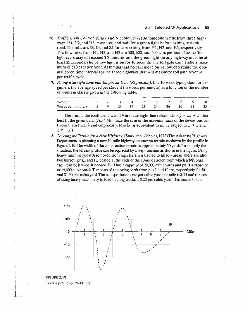
2.3 Selected LP Applications 65
*6. Traffic Light Control. (Stark and Nicholes, 1972) Automobile traffic from three highways, HI, H2, and H3, must stop and wait for a green light before exiting to a tollroad. TIle tolls are $3, $4, and $5 for cars exiting from HI, H2, and H3, respectively.The flow rates from HI, H2, and H3 are 500,600, and 400 cars per hour. The trafficlight cycle may not exceed 2.2 minutes, and the green light on any highway must be atleast 25 seconds. The yellow light is on for 10 seconds. The toll gate can handle a maximum of 510 cars per hour. Assuming that no cars move on yellow, determine the optimal green time interval for the three highways that will maximize toll gate revenueper traffic cycle.
7. Filling a Straight Line into Empirical Data (Regression). In a lO-week typing class for beginners, the average speed per student (in words per minute) as a function of the numberof weeks in class is given in the following table.
Week,xWords per minute, y
15
29
315
419
521
624
726
830
931
1035
Determine the coefficients a and b in the straight-line relationship, y = ax + b, thatbest fit the given data. (Hint: Minimize the sum of the absolute value of the deviations between theoretical yand empirical y. Min Ixl is equivalent to min z subject to z :s x andz ~ -x.)
8. Leveling the Terrain for a New Highway. (Stark and Nicholes, 1972) The Arkansas HighwayDepartment is planning a new 10-mile highway on uneven terrain as shown by the profile inFigure 2.10.The width of the construction terrain is approximately 50 yards. To simplify thesituation, the terrain profile can be replaced by a step function as shown in the figure. Usingheavy machinery, earth removed from high terrain is hauled to fill low areas. There are alsotwo burrow pits, I and II, located at the ends of the lO-mile stretch from which additionalearth can be hauled, if needed. Pit I has a capacity of 20,000 cubic yards and pit II a capacityof 15,000 cubic yards. TIle costs of removing earth from pits I and II are, respectively, $1.50and $1.90 per cubic yard. The transportation cost per cubic yard per mile is $.15 and the costof using heavy machinery to load hauling trucks is $.20 per cubic yard. This means that a
+20
+100
o
-10
-20
FIGURE 2.10
f- "J \"I \ , "'\ , ,,
\,\
J ,I , ,
I , ,I II , I I 10
I I, I, , I I
,I I I
1 3 5 7 8 9,,
I \ /
I /, J I ,I I ,
II
, ,, ,- ,
I I \ /,,I \ ,
I I "' ~
,I
, --II
f- ,I II ,I II I\,
Mile
ti.i:
l ..
Terrain profile for Problem 8
66 Chapter 2 Modeling with linear Programming
cubic yard from pit I hauled one mile will cost a total of (1.5 + .20) + 1 X .15 = $1.85 anda cubic yard hauled one mile from a hill to a fill area will cost .20 + 1 x .15 = $.35. Develop a minimum cost plan for leveling the lO-mile stretch.
9. Military Planning. (Shepard and Associates, 1988) The Red Army (R) is trying to invadethe territory defended by the Blue Army (B). Blue has three defense lines and 200 regular combat units and can draw also on a reserve pool of 200 units. Red plans to attack ontwo fronts, north and south, and Blue has set up three east-west defense lines, I, II, andIII. The purpose of defense lines I and II is to delay the Red Army attack by at least 4days in each line and to maximize the total duration of the battle. The advance time ofthe Red Army is estimated by the following empirical formula:
. . (Blue units)Battle duratIon In days = a + b R .ed umts
The constants a and b are a function of the defense line and the north/south front asthe following table shows:
North frontSouth front
I
.51.1
a
II
.751.3
III
.551.5
I
8.810.5
b
II
7.98.1
III
10.29.2
The Blue Army reserve units can be used in defense lines II and II only. The allocation of units by the Red Army to the three defense lines is given in the following table.
Number of Red Army attack units
North frontSouth front
DefellSe Line I
3030
Defense Line 1I
6040
Defense Line III
2020
How should Blue allocate its resources among the three defense lines and thenorth/south fronts?
10. Water Quality Management. (Stark and Nicholes, 1972) Four cities discharge waste waterinto the same stream. City 1 is upstream, followed downstream by city 2, then city 3, thencity 4. Measured alongside the stream, the cities are approximately 15 miles apart. Ameasure of the amount of pollutants in waste water is the BOD (biochemical oxygen demand), which is the weight of oxygen required to stabilize the waste constituent in water.A higher BOD indicates worse water quality. TIle Environmental Protection Agency(EPA) sets a maximum allowable BOD loading, expressed in lb BOD per gallon. The removal of pollutants from waste water takes place in two forms: (1) natural decompositionactivity stimulated by the oxygen in the air, and (2) treatment plants at the points of discharge before the waste reaches the stream. The objective is to determine the most economical efficiency of each of the four plants that will reduce BOD to acceptable levels.The maximum possible plant efficiency is 99%.
To demonstrate the computations involved in the process, consider the following definitions for plant 1:
QI = Stream flow (gal/hour) on the IS-mile reach 1-2 leading to city 2
PI = BOD discharge rate (in lb/hr)
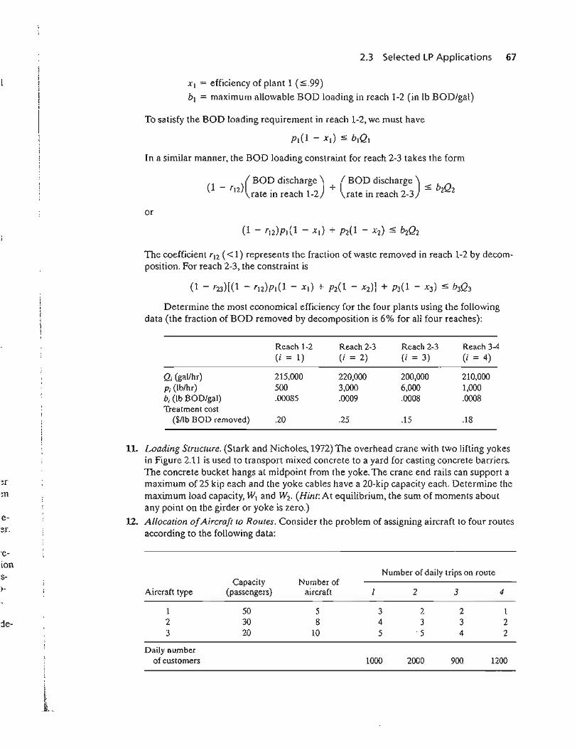
~r
~n
e-er.
'eions1-
:le-
2.3 Selected lP Applications 67
XI = efficiency of plant 1 (:::;.99)
bi = maximum allowable BOD loading in reach 1-2 (in lb BOD/gal)
To satisfy the BOD loading requirement in reach 1-2, we must have
PI(l - xd :::; b1QI
In a similar manner, the BOD loading constraint for reach 2-3 takes the form
(BOD diSCharge) ( BOD diSCharge)
1 - Tl2. +. :::; b Q( ) rate In reach 1-2 rate In reach 2-3 2 Z
or
The coefficient Tl2 «1) represents the fraction of waste removed in reach 1-2 by decomposition. For reach 2-3, the constraint is
Determine the most economical efficiency for the four plants using the followingdata (the fraction of BOD removed by decomposition is 6% for all four reaches):
Reach 1-2 Reach 2-3 Reach 2-3 Reach 3-4(i == 1) (i == 2) (i = 3) (i = 4)
Qi (gal/hr) 215,000 220,000 200,000 210,000Pi (Ib/hr) 500 3,000 6,000 1,000hi (Ib BOD/gal) .00085 .0009 .0008 .0008Treatment cost
($/Ib BOD removed) .20 .25 .15 .18
11. Loading Structure. (Stark and Nicholes, 1972) The overhead crane with two lifting yokesin Figure 2.11 is used to transport mixed concrete to a yard for casting concrete barriers.The concrete bucket hangs at midpoint from the yoke. The crane end rails can support amaximum of 25 kip each and the yoke cables have a 20-kip capacity each. Determine themaximum load capacity, WI and Wz. (Hint: At equilibrium, the sum of moments aboutany point on the girder or yoke is zero.)
12. Allocation ofAircraft to Routes. Consider the problem of assigning aircraft to four routesaccording to the following data:
Number of daily trips on routeCapacity Number of
Aircraft type (passengers) aircraft I 2 3 4
1 50 5 3 2 2 12 30 8 4 3 3 23 20 10 5 5 4 2
Daily numberof customers 1000 2000 900 1200
68 Chapter 2 Modeling with Linear Programming
....1 2 fl L 6 ft ----+I,''0+'-- 8 ft 12 ft ------+I.' 2 ft I- 2
Yoke 1
FIGURE 2.11
Overhead crane with two yokes (Problem 11)
.
.Yoke 2 :. .
l:i,~:~b~:~~~~'££§~~tp~,;~(~~~~~I
TIle associated costs, including the penalties for losing customers because of spaceunavailability, are
Operating cost ($) per trip on route
Aircraft type 1 2 3 4
1 1000 1100 1200 15002 800 900 1000 10003 600 800 800 900
Penalty ($) perlost customer 40 50 45 70
Determine the optimum allocation of aircraft to routes and determine the associatednumber of trips.
2.4 COMPUTER SOLUTION WITH SOLVER AND AMPL
In practice, where typical linear programming models may involve thousands of vari~
abies and constraints, the only feasible way to solve such models is to use the computer. This section presents two distinct types of popular software: Excel Solver andAMPL. Solver is particularly appealing to spreadsheet users. AMPL is an algebraicmodeling language that, like any other programming language, requires more expertise. Nevertheless, AMPL, and other similar languages,3 offer great flexibility in modeling and executing large and complex LP models. Although the presentation in thissection concentrates on LPs, both AMPL and Solver can be used with integer and nonlinear programs, as will be shown later in the book.
30ther known commercial packages include AfMMS, GAMS, LINGO, MPL. OPL Studio, and Xpress-Mosel.
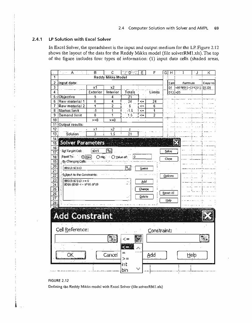
2.4 Computer Solution with Solver and AMPL 69
2.4.1 LP Solution with Excel Solver
In Excel Solver, the spreadsheet is the input and output medium for the LP. Figure 2.12shows the layout of the data for the Reddy Mikks model (file solverRM1.xls).111e topof the figure includes four types of information: (1) input data cells (shaded areas,
A'··1
-2 . In ut data: Cell formula Copy to
. ~ - ...._···Oo.... I-E"---x-;-e:-io-r-+--ln-t:-;-io-r-l·--TotaIS··'--'·' --Li;-iJits!-·· ~3' :~i~~~~~·?~S2?~~:P~...:5;:; Ob'ective 5 4 21 . _.:, . ,
1----'.::6'-+::R:..=a:L:w
=--=m::.:.:.a-=-te-ri=-a---:-I---:-1+------:6=----f--4-:-----,1--...:2~4:....-(&-<-=---i--2=-4-:------! .. --:. -.-- -----.- - - ;-- '0__ :
7' Raw material 2 1 2 6 6... ,........•.. __ 1.. '
S' Markel limit .1 1 ·1.5 1:: '; ,i--------=--+.:;==:..:.:.::,=--+--.,:----jf--------------'----t------.-- .... -... ·--·c..--- ...- .....------ :"--.•••-- .•.••• --... ,9 Demand limit 0 1 1.5 <= 210 >=0 >=0
i.. .. .. ... ,~. ..,12 x1 x2 z .
13 .·.·...·.·.·_S.o._lu.l_·io.·li ..._.. _·-·Je.-.....;;.3_....;..._1,;,,;,.:l.;..-_.,...-....;;;,2.;..1_[·----; --.--- ... i -- "","--" .._... ;-.- --.---j ----.- :-- ,-----:._------------+.·-1---1--- .. --- _L -- .~I •• - --
11 Out Jut results:
i.. ; .....
-_._-_._-~. --_._-~-_.. -_.__ . _.:___ •••_••• L_ ••••_..... 'M"
, I
__ 1..__ ._ ..!.,
'--'- -,. r-- - -.- ~ - -_ ,.- _H,,---- _.. :.. _.. ; - ~
~.. .i..._.._~. __ ..:
. I--_._- ._'-~ ..- ; -.. _.__.-.
Help ... --.--- ... u'.'
Close I. .uu' -:. ----.. '1----..
Qplions
B,esel.t..l1
; S8S13:~CS13 >= 0SoS6:g)~ <= sF::-6:sFS9
>5l,!bject 1lJ the Constraints:t· .
. S~tTaraetCeJl:" [i)~~."EQuaJT:o: "... 0J&~;(] O"'!iciO:Lalueof.:··~--J(~I changirlg Cells: ._.....-...._-.. '-"'~""~" ...-. --_._.. .., -.. - ... _,....,#_.•••_0_. ~- ..-~ . '. . .
1Isas13:SCS13
161718.19'202122232425 .262728
]
[~
Help[
Constraint:'
AddCancel
Cell Reference:
~~-~=n:~
'---------------.,;
"'---""-"'-'-'--~~>=...-----......-"""""',-----lint I--I...----~-----..
! bJ'n ..,~/. i I ~'--'.' '-.-.-----------.. --- -------- .uoo .. !----------- __-.---.-- ."-=-'-'---__--'--.-.---r.oo--.----.-.--oo--.-. __ .. ,. .oo, 00.'..-.-...-....... .... ..
FIGURE 2.12
Defining the Reddy Mikks model with Excel Solver (file solverRMl.xls)
t.
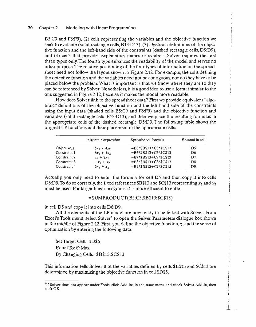
70 Chapter 2 Modeling with Linear Programming
B5:C9 and F6:F9), (2) cells representing the variables and the objective function weseek to evaluate (solid rectangle cells, B13:013), (3) algebraic definitions of the objective function and the left-hand side of the constraints (dashed rectangle cells, 05:09),and (4) cells that provides explanatory names or symbols. Solver requires the firstthree types only. The fourth type enhances the readability of the model and serves noother purpose. The relative positioning of the four types of information on the spreadsheet need not follow the layout shown in Figure 2.12. For example, the cells definingthe objective function and the variables need not be contiguous, nor do they have to beplaced below the problem. What is important is that we know where they are so theycan be referenced by Solver. Nonetheless, it is a good idea to use a format similar to theone suggested in Figure 2.12, because it makes the model more readable.
How does Solver link to the spreadsheet data? First we provide equivalent "algebraic" definitions of the objective function and the left-hand side of the constraintsusing the input data (shaded cells B5:C9 and F6:F9) and the objective function andvariables (solid rectangle cells B13:013), and then we place the resulting formulas inthe appropriate cells of the dashed rectangle D5:09. The following table shows theoriginal LP functions and their placement in the appropriate cells:
Objective, Z
Constraint 1Constraint 2Constraint 3Constraint 4
Algebraic expression
5Xl + 4.x2
6x( + 4X2
XI + 2X2
-.xl + X2
OXI + X2
Spreadsheet formula
=BS*$B$13+C5*$C$13=B6*$B$13+C6*$C$13=B7*$B$13+C7*$C$13=B8*$B$13+C8*$C$13=B9*$B$13+C9*$C$ J3
Entered in cell
DSD6D7D8D9
Actually, you only need to enter the formula for cell 05 and then copy it into cellsD6:09. To do so correctly, the fixed references $B$13 and $C$13 representing Xl and X2
must be used. For larger linear programs, it is more efficient to enter
=SUMPROOUCf(B5:C5,$B$13:$C$13)
in cell D5 and copy it into cells D6:D9.All the elements of the LP model are now ready to be linked with Solver. From
Excel's Tools menu, select Solver4 to open the Solver Parameters dialogue box shownin the middle of Figure 2.12. First, you define the objective function, z, and the sense ofoptimization by entering the following data:
Set Target Cell: $D$5Equal To: 0 MaxBy Changing Cells: $B$13:$C$13
This information tells Solver that the variables defined by cells $B$13 and $C$13 aredetermined by maximizing the objective function in cell $D$5.
4If Solver does not appear under Tools, click Add-ins in the same menu and check Solver Add-in, thenclick OK.
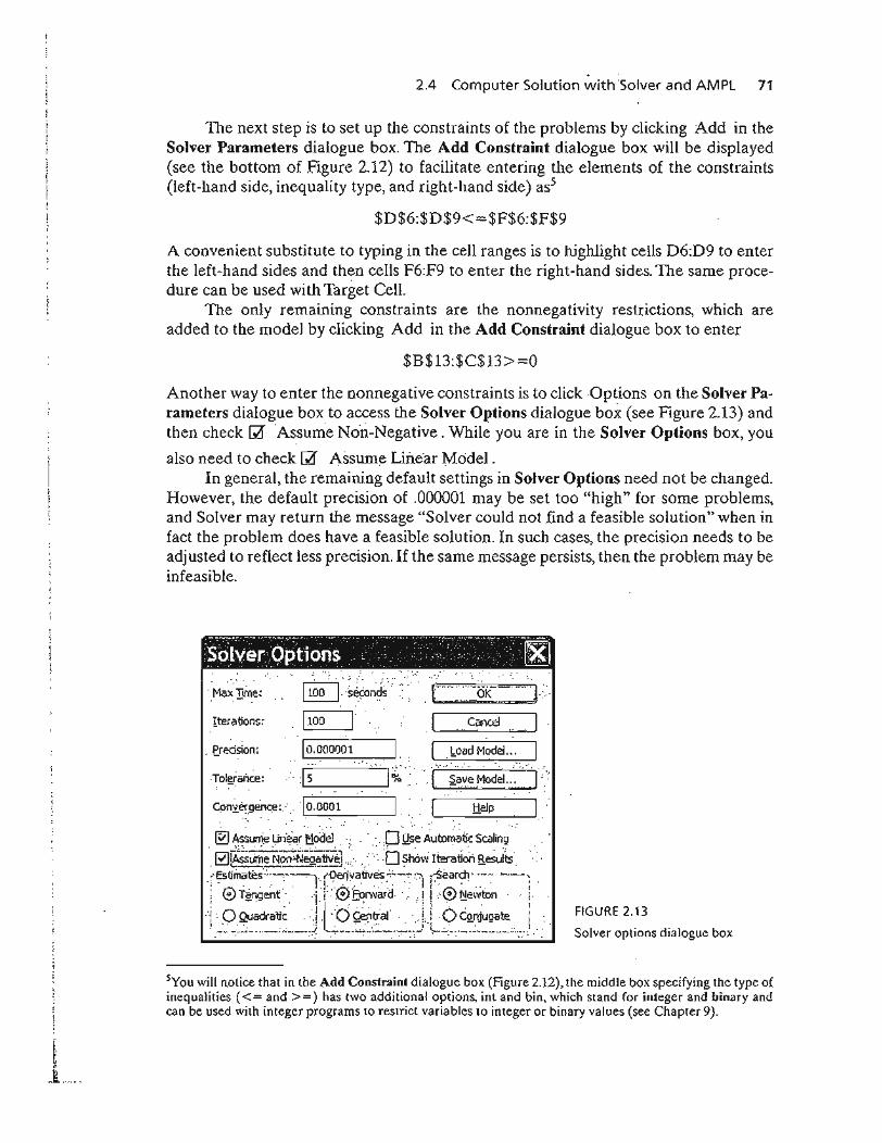
2.4 Computer Solution with Solver and AMPL 71
TIle next step is to set up the constraints of the problems by clicking Add in theSolver Parameters dialogue box. The Add Constraint dialogue box will be displayed(see the bottom of Figure 2.12) to facilitate entering the elements of the constraints(left-hand side, inequality type, and right-hand side) ass
$D$6:$D$9<=$F$6:$F$9
A convenient substitute to typing in the cell ranges is to highlight cells D6:D9 to enterthe left-hand sides and then cells F6:F9 to enter the right-hand sides. The same procedure can be used with Target Cell.
The only remaining constraints are the nonnegativity restrictions, which areadded to the model by clicking Add in the Add Constraint dialogue box to enter
$B$13:$C$13>=0
Another way to enter the nonnegative constraints is to click Options on the Solver Parameters dialogue box to access the Solver Options dialogue box (see Figure 2.13) andthen check r;;r Assume Non-Negative. While you are in the Solver Options box, you
also need to check r;;r Assume Linear Model.In general, the remaining default settings in Solver Options need not be changed.
However, the default precision of .000001 may be set too "high" for some problems,and Solver may return the message "Solver could not find a feasible solution" when infact the problem does have a feasible solution. In such cases, the precision needs to beadjusted to reflect less precision. If the same message persists, then the problem may beinfeasible.
MaxIime:
Iterations:
.e.redsion:
Tol~ance:
'~'b~¢onJS:i' .C·::~6jC ·~:···::r·
1100 I I Cancel I .[QOOOOO_l_....".....-J J.booad t-lodei... I.
'1_5_._..--.,.._._.. '_", ~~.:' (~~V~}~Od~L."~.·.J·c
Q:;nyergence:<!o.OOOl I' I Help I.f
e
~A§~~ Unear M~:dcl .'..... ..DQ~ AU~tic scaling'
.o~S~fl2i;~~9~rr:::'J:·~~:_-;; €)Tangent ·:i.@Forwardi LeNe,\.ton .. :, -'.. [·i· .-, ,";' -. ;1..0Quadratic 'Jrd ~entJ:a1itl 0 c~njugate !
._~~.•: .• ~.: __•.: ..: __._~:~ -:-__ ..~.. ~.~ .~.-:'-,O~':_. l:_• .:-,_ .!_,••_._.:..- .•.:::.__ ' .
FIGURE 2.13
Solver options dialogue box
:nSYou will notice that in the Add Constraint dialogue box (Figure 2.12), the middle box specifying the type ofinequalities « = and> =) has two additional options, int and bin, which stand for integer and binary andcan be used with integer programs to restrict variables 10 integer or binary values (see Chapter 9).
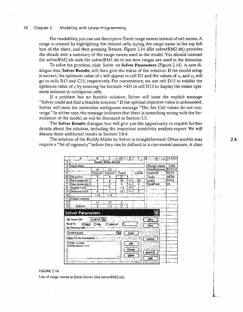
72 Chapter 2 Modeling with Linear Programming
For readability, you can use descriptive Excel range names instead of cell names. Arange is created by highlighting the desired cells, typing the range name in the top leftbox of the sheet, and then pressing Return. Figure 2.14 (file solverRM2.xls) providesthe details with a summary of the range names used in the model. You should contrastfile solverRM2.xls with file solverRM1.xls to see how ranges are used in the formulas.
To solve the problem, click Solve on Solver Parameters (figure 2.14). A new dialogue box, Solver Results, will then give the status of the solution. If the model setupis correct, the optimum value of z will appear in cell D5 and the values of Xl and X2 willgo to cells B13 and C13, respectively. For convenience, we use cell Dl3 to exhibit theoptimum value of z by entering the formula =D5 in cell DB to display the entire optimum solution in contiguous cells.
If a problem has no feasible solution, Solver will issue the explicit message"Solver could not find a feasible solution." If the optimal objective value is unbounded,Solver will issue the somewhat ambiguous message "The Set Cell values do not converge." In either case, the message indicates that there is something wrong with the formulation of the model, as will be discussed in Section 3.5.
TIle Solver Results dialogue box will give you the opportunity to request furtherdetails about the solution, including the important sensitivity analysis report. We willdiscuss these additional results in Section 3.6.4.
The solution of the Reddy Mikks by Solver is straightforward. Other models mayrequire a "bit of ingenuity" before they can be defined in a convenient manner. A class
.. A " '·>cs·' C>·' ::;·~'D'\';~:IEJ" ',F\:IGkii:.::'·:Hi>.t~~;i~;~~~l'ij.1d
,·f. Reddv Mikks Model . ,. !....2.',. Input data: i Range name Cells
+-_.----. "... Ex~1rior hlt:;ior 'To'ta'j;':' -'hJlnit~r ij~f:-~~~~ldu~es! ~~~$? Objective 5 4 21 i'-j' ·_·_..·..t' iOlals ....,.' 06:09'6'. Raw material 1 6 4 I 24 1<= 14 i GiYiliS----' F6:F9T Raw material 2 1 2 !-.~-.'~=-:~ <= 6': TolalPrafit 05
1~O ~:::I~~i~l~it >L >~o :"':H--::: .~ ;)~~~'~~~,~~~.-~~ --J*O",:;:;'~ I~' ;~ ;, ii-nir:~::~~[j
:~(r~~;ceU:'IT taIPr fi@]"',: ' .. ,', ',:'CSoi r--E..--4
FIGURE 2.14
Use of range names in Excel Solver (file solverRM2.xls)
2.4.
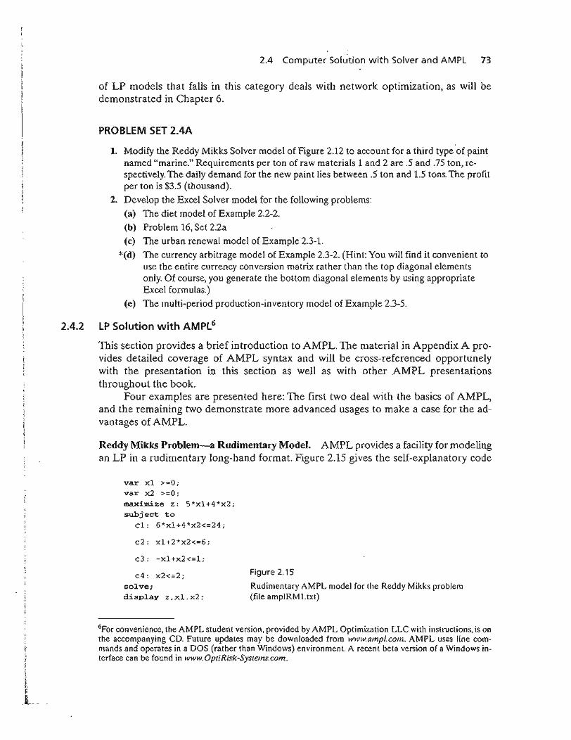
2.4 Computer Solution with Solver and AMPL 73
of LP models that falls in this category deals with network optimization, as will bedemonstrated in Chapter 6.
PROBLEM SET 2.4A
1. Modify the Reddy Mikks Solver model of Figure 2.12 to account for a third type of paintnamed "marine." Requirements per ton of raw materials 1 and 2 are .5 and .75 ton, respectively. The daily demand for the new paint lies between .5 ton and 1.5 tons. The profitper ton is $3.5 (thousand).
2. Develop the Excel Solver model for the following problems:
(a) The diet model of Example 2.2-2.
(b) Problem 16, Set 2.2a
(c) The urban renewal model of Example 2.3-1.
*(d) The currency arbitrage model of Example 2.3-2. (Hint: You will find it convenient touse the entire currency conversion matrix rather than the top diagonal elementsonly. Of course, you generate the bottom diagonal elements by using appropriateExcel formulas.)
(e) The multi-period production-inventory model of Example 2.3-5.
2.4.2 lP Solution with AMPl6
This section provides a brief introduction to AMPL. The material in Appendix A provides detailed coverage of AMPL syntax and will be cross-referenced opportunelywith the presentation in this section as well as with other AMPL presentationsthroughout the book.
Four examples are presented here: The first two deal with the basics of AMPL,and the remaining two demonstrate more advanced usages to make a case for the advantages of AMPL.
Reddy Mikks Problem-a Rudimentary Model. AMPL provides a facility for modelingan LP in a rudimentary long-hand format. Figure 2.15 gives the self-explanatory code
var xl >=0;
var x2 >=0;
maximize z: 5*xl+4*x2;subject to
cl: 6*xl+4*x2<=24;
c2: xl+2*x2<=6;
c3: -xl+x2<=1;
c4: x2<=2;solve;display z,xl,x2;
Figure 2.15
Rudimentary AMPL model for the Reddy Mikks problem(file ampIRM1.txt)
6For convenience, the AMPL student version, provided by AMPL Optimization LLC with instructions, is onthe accompanying CD. Future updates may be downloaded from www.ampl.com. AMPL uses line commands and operates in a DOS (rather than Windows) environment. A recent beta version of a Windows interface can be found in www.OptiRisk-Syslems.com.
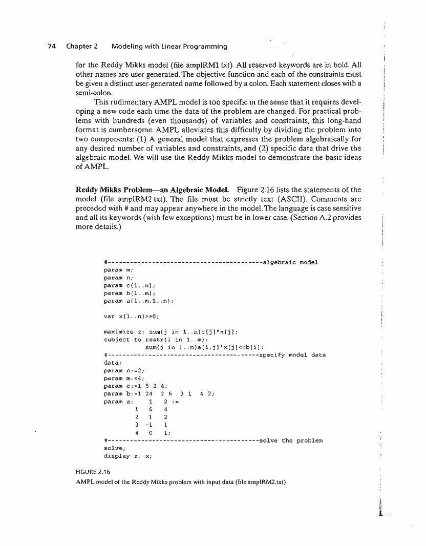
74 Chapter 2 Modeling with linear Programming
for the Reddy Mikks model (file ampIRM1.txt). All reserved keywords are in bold. Allother names are user generated. The objective function and each of the constraints mustbe given a distinct user-generated name followed by a colon. Each statement closes with asemi-colon.
This rudimentary AMPL model is too specific in the sense that it requires developing a new code each time the data of the problem are changed. For practical problems with hundreds (even thousands) of variables and constraints, this long-handformat is cumbersome. AMPL alleviates this difficulty by dividing the problem intotwo components: (1) A general model that expresses the problem algebraically forany desired number of variables and constraints, and (2) specific data that drive thealgebraic model. We will use the Reddy Mikks model to demonstrate the basic ideasofAMPL.
Reddy Mikks Problem-an Algebraic Model. Figure 2.16 lists the statements of themodel (file ampIRM2.txt). The file must be strictly text (ASCII). Comments arepreceded with # and may appear anywhere in the model. The language is case sensitiveand all its keywords (with few exceptions) must be in lower case. (Section A.2 providesmore details.)
#------------------------------------------algebraic modelparam m;param n;param c{l. .n};param b{1 .. m};param a{1. .m, 1. .n};
var x{l. .n) >=0;
maximize z: surn{j in 1. .n}c[jJ*x[jJ;subject to restr{i in 1 .. m):
sum{j in 1..n}a[i,jJ*x[jJ<=b[iJ;#-----------------------------------------specify model datadata;param n:=2;param m: =4;param c:=1 5 2 4;param b:=1 24 2 6 3 1 4 2;param a: 1 2.-
1 6 42 1 23 -1 14 0 1;
#-----------------------------------------solve the problemsolve;display z, x;
FIGU~E 2.16
AMPL model of the Reddy Mikks problem with input data (file ampIRM2.txt)
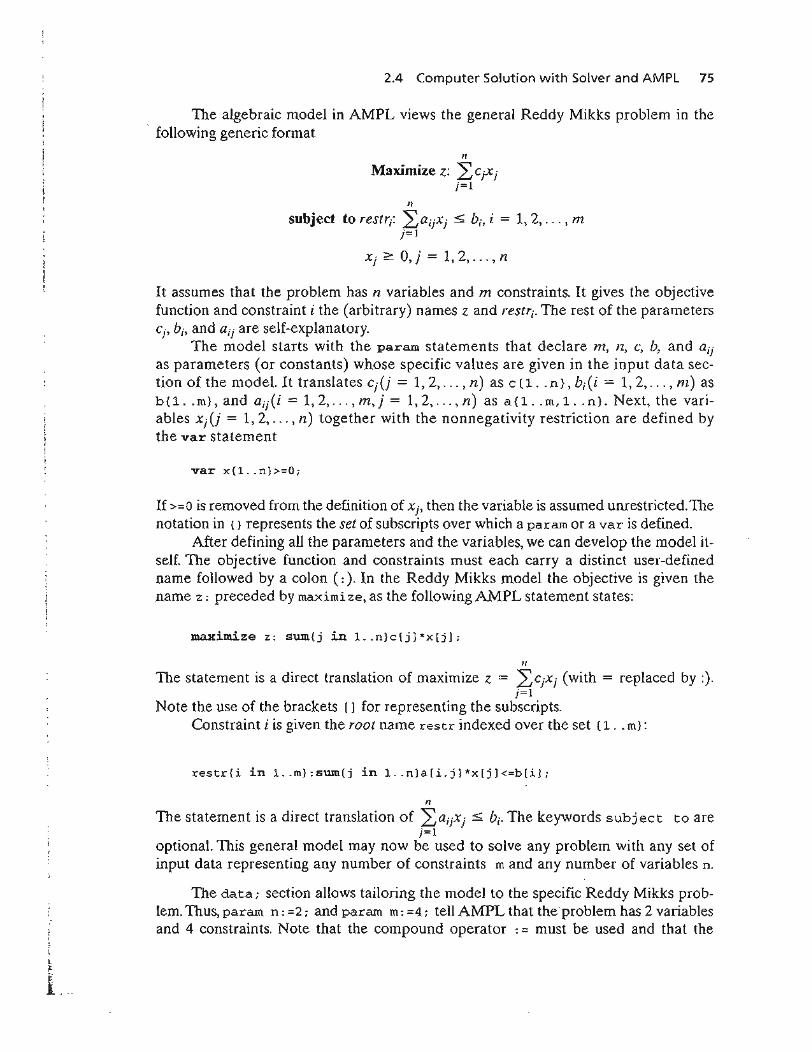
2.4 Computer Solution with Solver and AMPL 75
The algebraic model in AMPL views the general Reddy Mikks problem in thefollowing generic format
/I
Maximize z: L CjX jj=l
II
subject to restri: 2:aijXj < bi, i = 1, 2, ... , mj=l
Xj ~ 0, j = 1,2, ... , n
It assumes that the problem has n variables and m constraints. It gives the objectivefunction and constraint i the (arbitrary) names z and restrj. The rest of the parametersCj, bi> and aij are self-explanatory.
The model starts with the param statements that declare m, 11., C, b, and aij
as parameters (or constants) whose specific values are given in the input data sec-tion of the modeL It translates Cj(j = 1,2, , n) as c {1. . n}, bi (i = 1,2, ... , m) asb{1. .m}, and aij(i = 1,2, ... ,111.,j = 1,2, ,n) as a{1 .. m,1. .n}. Next, the vari-ables Xj (j = 1,2, ... , n) together with the nonnegativity restriction are defined bythe var statement
var x(I. .n}>=O;
If >=0 is removed from the definition of Xj' then the variable is assumed unrestricted.Thenotation in {} represents the set of subscripts over which a param or a var is defined.
After defining all the parameters and the variables, we can develop the model itself. The objective function and constraints must each carry a distinct user-definedname followed by a colon (:). In the Reddy Mikks model the objective is given thename z: preceded by maximi ze, as the following AMPL statement states:
maximize z: sum(j in 1. .n}c[jJ*x(j];
1/
The statement is a direct translation of maximize z = :2>jXj (with = replaced by:).j=l
Note the use of the brackets [] for representing the subscripts.Constraint i is given the root name restr indexed over the set {1 .. m}:
restr(i in I..m}:sum(j in l..n}a[i,j}*x[jl<=b[i];
/1
The statement is a direct translation of ~aijXj < bi' The keywords subject to arej=l
optional. This general model may now be used to solve any problem with any set ofinput data representing any number of constraints m and any number of variables n.
The data; section allows tailoring the model to the specific Reddy Mikks problem. Thus, param n: =2; and param m: =4; tell AMPL that the problem has 2 variablesand 4 constraints. Note that the compound operator : = must be used and that the
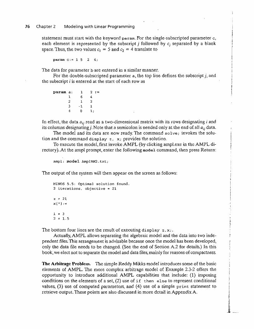
76 Chapter 2 Modeling with Linear Programming
statement must start with the keyword paramo For the single-subscripted parameter c,each element is represented by the subscript j followed by Cj separated by a blankspace.TI1Us, the two values CI = 5 and C2 = 4 translate to
param c:= 1 5 2 4;
The data for parameter b are entered in a similar manner.For the double-subscripted parameter a, the top line defines the sUbscript j, and
the subscript i is entered at the start of each row as
param a: 1 2 :=1 6 42 1 23 -1 14 0 1;
In effect, the data aij read as a two-dimensional matrix with its rows designating i andits columns designatingj. Note that a semicolon is needed only at the end of all aij data.
The model and its data are now ready. The command solve; invokes the solution and the command display z, X; provides the solution.
To execute the model, first invoke AMPL (by clicking ampI.exe in the AMPL directory). At the ampl prompt, enter the following model command, then press Return:
ampl: model AmplRM2. txt;
The output of the system will then appear on the screen as follows:
MINOS 5.5: Optimal solution found.2 iterations, objective = 21
z = 21x[*] :=
1 32 1. 5
The bottom four lines are the result of executing display z, x; .
Actually, AMPL allows separating the algebraic model and the data into two independent files. This arrangement is advisable because once the model has been developed,only the data file needs to be changed. (See the end of Section A.2 for details.) In thisbook, we elect not to separate the model and data files, mainly for reasons of compactness.
The Arbitrage Problem. The simple Reddy Mikks model introduces some of the basicelements of AMPL. The more complex arbitrage model of Example 2.3-2 offers theopportunity to introduce additional AMPL capabilities that include: (1) imposingconditions on the elements of a set, (2) use of if then else to represent conditionalvalues, (3) use of computed parameters, and (4) use of a simple print statement toretrieve output. These points are also discussed in more detail in Appendix A.
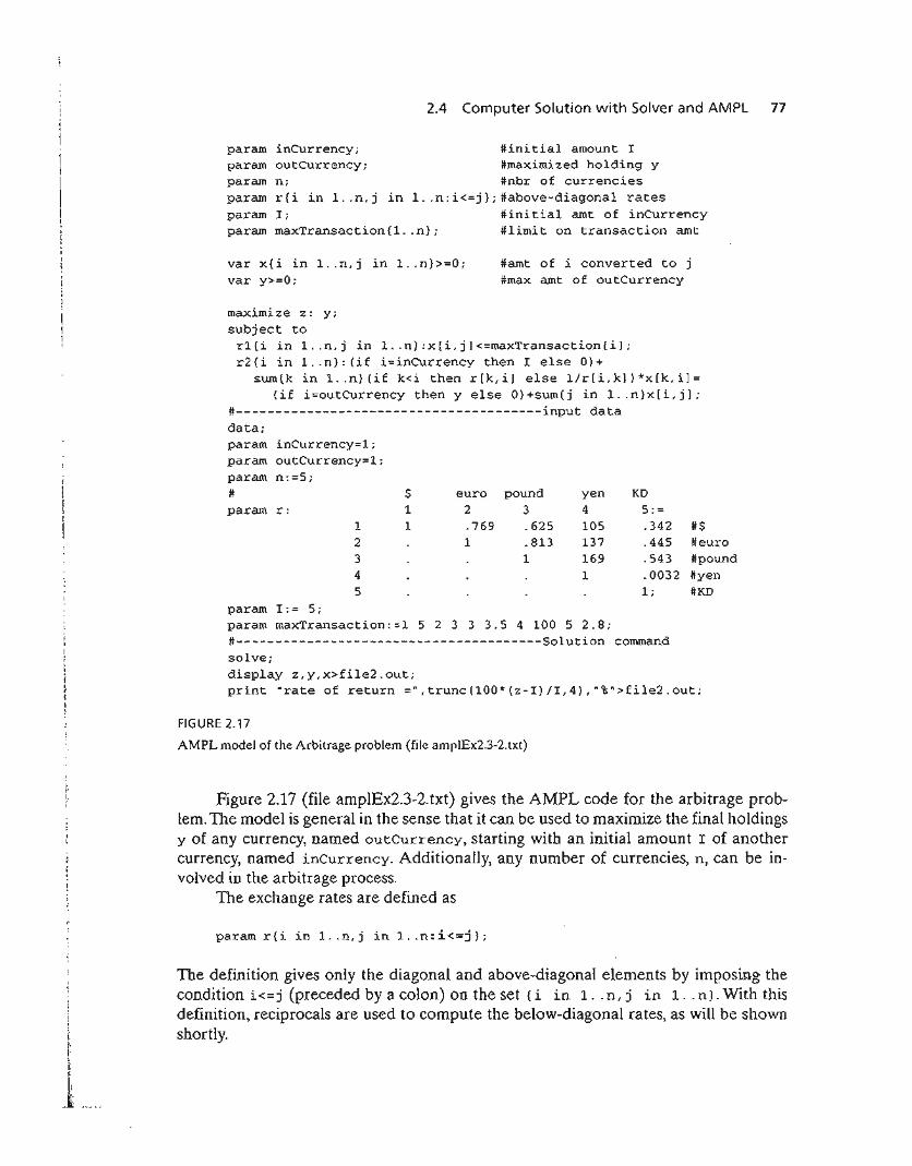
2.4 Computer Solution with Solver and AMPL 77
maxTransaction(l .. n};
rei in 1 .. n, j
inCurrency;outCurrency;
paramparamparam n;paramparam I;
param
#initial amount I#maximized holding y#nbr of currencies
in 1 ..n:i<=j};#above-diagonal rates#initial amt of inCurrency#limit on transaction amt
var x{i in 1 .. n,j in 1 .. n}>=O;var y>=O;
#amt of i converted to j#max arnt of outCurrency
#$#euro#pound#yen#KD1;
KD5:=.342.445.543.0032
yen4
105137
1691
pound3.625.813
1
2.7691
euro$1
1123
45
inCurrency=l;outCurrency=l;n:=5;
param r:
maximi ze z: y;
subject torl{i in 1 .. n,j in 1 .. n}:x[i,j]<=maxTransaction[i];r2{i in 1 .. n}:(if i=inCurrency then I else 0)+
sum{k in 1 .. n}(if k<i then r[k,i] else l/r[i,k])*x[k,i]=(if i=outCurrency then y else O)+sum{j in 1 .. n}x[i,j];
#---------------------------------------input datadata;paramparamparam#
param 1:= 5;param maxTransaction:=l 5 2 3 3 3.5 4 100 5 2.8;#---------------------------------------Solution commandsolve;display z,y,x>file2.out;print "rate of return =",trunc(100*(z-I)/I,4) ,"%">file2.out;
FIGURE 2.17
AMPL model of the Arbitrage problem (file ampIEx2.3-2.txt)
Figure 2.17 (file ampIEx2.3-2.txt) gives the AMPL code for the arbitrage problem. The model is general in the sense that it can be used to maximize the final holdingsy of any currency, named outCurrency, starting with an initial amount I of anothercurrency, named inCurrency. Additionally, any number of currencies, n, can be involved in the arbitrage process.
The exchange rates are defined as
param r{i in 1. .n,j in 1. .n:i<=j];
The definition gives only the diagonal and above-diagonal elements by imposing thecondition i<=j (preceded by a colon) on the set (i in 1 .. n, j in 1 .. n). With thisdefinition, reciprocals are used to compute the below-diagonal rates, as will be shownshortly.
78 Chapter 2 Modeling with Linear Programming
The variable Xij' representing the amount of currency i converted to currency j, isdefined as
var x{i in 1 .. n,j in 1 .. n»=0;
The model has two sets of constraints: The first set with the root name rl sets thelimits on the amounts of any currency conversion transaction by using the statement
r1{i in 1 .. n,j in 1 .. n}: x[i,j]<=maxTransaction[i];
The second set of constraints with the root name r2 is a translation of the restriction
(Input to currency i) = (Output from currency i)
Its statement is given as
r2{i in 1 .. n} :(if i=inCurrency then I else 0)+sum{k in l .. n}{if k<i then r[k,i] else l/r[i,k])*x[k,i]
=(if i=outCurrency then y else O)+surn{j in 1 .. n}x[i,j];
This type of constraints is ideal for the use of the special construct if then else tospecify conditional values. In the left-hand side of the constraint, the expression
(if i=inCurrency then 1 else 0)
says that in the constraint for the input currency (i=inCurrency) there is an externalinput I, else the external input is zero. Next, the expression
sum{k in l .. n} (if k<i then r[k,i] else 1/r[i,kJ)*x[k,i]
computes the input funds from other currency converted to the input currency. If youreview Example 2.3-2 you will notice that when k<i, the conversion uses the abovediagonal elements of the exchange rate r. Otherwise, the row reciprocal is used for thebelow-diagonal elements (diagonal elements are 1). This is precisely what if then
else does. (See Section A.3 for details.)The if-expression in the right-hand side of constraint r2 can be explained in a
similar manner - namely,
(if i=outCurrency then y else 0)
says that the external output is y for outCurrency and zero for all others.We can enhance the readability of constraints r2 by defining the following
computed parameter (see Section A.3) that defines the entire exchange rate table:
Pararn rate(k in 1 .. n,i in 1 .. n}=(if k<i then r[k,iJ else l/r[i,k])
2.4 Computer Solution with Solver and AMPl 79
In this case, constraints r2 become
r2 {i in 1 .. n} :(if i=inCurrency then I else 0)+ sum(k in 1 .. n)rate[k,iJ*x[k,i]
=(if i=outCurrency then y else O)+sum(j in 1 .. n}x{i,j];
In the data; section, inCurrency and outCurrency each equal 1, which meansthat the problem is seeking the maximum dollar output using an initial amount of $5million. In general, inCurrency and outC\lrrency may designate any distinct currencies. For example, setting inCurrency equal to 2 and outCurrency equal to 4 maximizes the yen output given a 5 million euros initial investment.
The unspecified entries of param r are flagged in AMPL with dots (.). Thesevalues are then overridden either by using the reciprocal as shown in Figure 2.17 orthrough the use of the computed parameter ra te as shown above. The alternative tousing dots is to unnecessarily compute and enter the below-diagonal elements asdata.
The display statement sends the output to file file2.out instead of defaulting it tothe screen. The print statement computes and truncates the rate of return and sendsthe output to file file2.out. The print statement can also be formatted using printf,
just as in any higher level programming language. (See Section A.S.2 for details.)It is important to notice that input data in AMPL need not be hard-coded in the
model, as they can be retrieved from external files, spreadsheets, and databases (seeSection A.S for details). This is crucial in the arbitrage model, where the volatile exchange rates must often be accepted within less than 10 seconds. By allowing theAMPL model to receive its data from a database that automatically updates the exchange rates, the model can provide timely optimal solutions.
The Bus Scheduling Problem. The bus scheduling problem of Example 2.3-8 providesan interesting modeling situation in AMPL. Of course, we can always use a twosubscripted parameter, similar to parameter a in the Reddy Mikks model in Section 2.4.2(Figure 2.16), but this may be cumbersome in this case. Instead, we can take advantage ofthe special structure of the constraints and use conditional expressions to represent themimplicitly.
The left-hand side of constraint 1 is Xl + X,m where In is the total number of periods in a 24-hour day (= 6 in the present example). For the remaining constraints, theleft-hand side takes the form Xi-l + Xi> i = 2,3, ... , m. Using if then else (as wedid in the arbitrage problem), all In constraints can be represented compactly by onestatement as shown in Figure 2.18 (file amplEx2.3-8.txt). This representation is superior to defining the left-hand side of the constraints as an explicit parameter.
AMPL offers a wide range of programming capabilities. For example, theinput/output data can be secured from/sent to external files, spreadsheets, and databases and the model can be executed interactively for a wide variety of options thatallow testing different scenarios. The details are given in Appendix A. Also, manyAMPL models are presented throughout the book with cross references to the material in Appendix A to assist you in understanding these options.
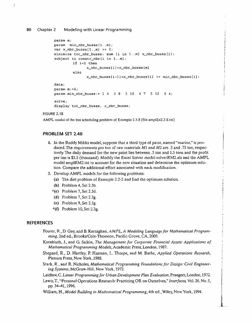
80 Chapter 2 Modeling with Linear Programming
param m;param min_nbr_buses{l .. m};var x_nbr_buses{l .. m} >= 0;minimize tot_nbr_buses: sum {i in 1 .. m} x_nbr_buses[i];subject to constr_nbr{i in 1 .. m}:
if i=l thenx_nbr_buses[iJ+x_nbr_buses[mJ
else
data;param m::=6;param min_nbr_buses:= 1 4 2 8 3 10 4 7 5 12 6 4;
solve;display tot_nbr_buses, x_nbr_buses;
FIGURE 2.18
AMPL model of the bus scheduling problem of Example 2.3-8 (file ampIEx2.3-8.txt)
PROBLEM SET 2.4B
1. In the Reddy Mikks model, suppose that a third type of paint, named "marine," is produced. The requirements per ton of raw materials M1 and M2 are .5 and.75 ton, respectively. The daily demand for the new paint lies between .5 ton and 1.5 tons and the profitper ton is $3.5 (thousand). Modify the Excel Solver model solverRM2.xls and the AMPLmodel amplRM2.txt to account for the new situation and determine the optimum solution. Compare the additional effort associated with each modification.
2. Develop AMPL models for the following problems:
(a) The diet problem of Example 2.2-2 and find the optimum solution.
(b) Problem 4, Set 2.3b.
*(c) Problem 7, Set 2.3d.
(d) Problem 7, Set 2.3g.
(e) Problem 9, Set 2.3g.
*(1) Problem 10, Set 2.3g.
REFERENCES
FoureT, R., D. Gay, and B. Kernighan, A MPL, A Modeling Language for Mathematical Programming,2nd ed., Brooks/Cole-Thomson, Pacific Grove, CA, 2003.
Kornblutb, 1., and G. Salkin, The Management for Corporate Financial Assets: Applications ofMathematical Programming Models, Academic Press, London, 1987.
Shepard, R., D. Hartley, P. Hasman, L. Thorpe, and M. Bathe, Applied Operations Research,Plenum Press, New York, 1988.
Stark, R., and R. Nicholes, Mathematical Programming Foundations for Design: Civil Engineering Systems, McGraw-Hili, New York, 1972.
Laidlaw, C. Linear Programming for Urban Development Plan Evaluation, Praegers, London, 1972.
Lewis, T., "Personal Operations Research: Practicing OR on Ourselves," Interfaces, Vol. 26, No.5,pp. 34--41, 1996.
William, H., Model Building in Mathematical Programming, 4th ed., Wiley, New York, 1994.
fI·f.Ir.
t
CHAPTER 3
The Simplex Methodand Sensitivity Analysis
Chapter Guide. This chapter details the simplex method for solving the general LPproblem. It also explains how simplex-based sensitivity analysis is used to provide important economic interpretations about the optimum solution, including the dual pricesand the reduced cost.
The simplex method computations are particularly tedious, repetitive, and, aboveall, boring. As you do these computations, you should not lose track of the big picture;namely, the simplex method attempts to move from one corner point of the solutionspace to a better corner point until the optimum is found. To assist you in this regard,TORA's interactive user-guided module (with instant feedback) allows you to decidehow the computations should proceed while relieving you of the burden of the tediouscomputations. In this manner, you get to understand the concepts without being overwhelmed by the computational details. Rest assured that once you have learned howthe simplex method works (and it is important that you do understand the concepts),computers will carry out the tedious work and you will never again need to solve an LPmanually.
Throughout my teaching experience, I have noticed that while students can easily carry out the tedious simplex method computations, in the end, some cannot tell whythey are doing them or what the solution is. To assist in overcoming this potential difficulty, the material in the chapter stresses the interpretation of each iteration in terms ofthe solution to the original problem.
When you complete the material in this chapter, you will be in a position to readand interpret the output reports provided by commercial software. The last section describes how these reports are generated in AMPL, Excel Solver, and TORA.
This chapter includes a summary of 1 real-life application, 11 solved examples,1 AMPL model, 1 Solver model, 1 TORA model, 107 end-of-section problems, and 3cases. The cases are in Appendix E on the CD. The AMPLlExcel/SolverITORA programs are in folder ch3Files.
81
82 Chapter 3 The Simplex Method and Sensitivity Analysis
Real Life Application-Optimization of Heart Valve Production
Biological heart valves in different sizes are bioprostheses manufactured from porcinehearts for human implantation. On the supply side, porcine hearts cannot be "produced" to specific sizes. Moreover, the exact size of a manufactured valve cannot be determined until the biological component of pig heart has been processed. As a result,some sizes may be overstocked and others understocked. A linear programming modelwas developed to reduce overstocked sizes and increase understocked sizes. The resulting savings exceeded $1,476,000 in 1981, the year the study was made. The details ofthis study are presented in Case 2, Chapter 24 on the CD.
3.1 LP MODEL IN EQUATION FORM
The development of the simplex method computations is facilitated by imposing tworequirements on the constraints of the problem:
1. All the constraints (with the exception of the nonnegativity of the variables) areequations with nonnegative right-hand side.
2. All the variables are nonnegative.
These two requirements are imposed here primarily to standardize and streamline thesimplex method calculations. It is important to know that all commercial packages(and TORA) directly accept inequality constraints, nonnegative right-hand side, andunrestricted variables. Any necessary preconditioning of the model is done internallyin the software before the simplex method solves the problem.
3.1.1 Converting Inequalities into Equations with NonnegativeRight-Hand Side
In (::;) constraints, the right-hand side can be thought of as representing the limit onthe availability of a resource, in which case the left-hand side would represent theusage of this limited resource by the activities (variables) of the model. The differencebetween the right-hand side and the left-hand side of the (::;) constraint thus yields theunused or slack amount of the resource.
To convert a (<:)-inequality to an equation, a nonnegative slack variable is addedto the left-hand side of the constraint. For example, in the Reddy Mikks model (Example2.1-1), the constraint associated with the use of raw material M1 is given as
6Xl + 4x2 <: 24
Defining Sl as the slack or unused amount of MI, the constraint can be converted tothe following equation: .
6X1 + 4X2 + Sl = 24, sl C: °Next, a (c: )-constraint sets a lower limit on the activities of the LP model, so that
the amount by which the left-hand side exceeds the minimum limit represents asurplus. The conversion from (~) to (:=) is achieved by subtracting a nonnegative
L
2.
3.
on:heIcethe
*4.ledpie
e)-
t,~l
/0
re
he;esndlly
I to
:hatts a
tive
L
3.1 LP Model in Equation Form 83
surplus variable from the left-hand side of the inequality. For example, in the dietmodel (Example 2.2-2), the constraint representing the minimum feed requirements is
xl + x2 2: 800
Defining Sl as the surplus variable, the constraint can be converted to the followingequation
Xl + X2 - SI = 800, Sl > 0
The only remaining requirement is for the right-hand side of the resulting equation to be nonnegative. The condition can always be satisfied by multiplying both sidesof the resulting equation by -1, where necessary. For example, the constraint
-Xl + X2 <: -3
is equivalent to the equation
- Xl + X2 + Sl = -3, SI 2': 0
Now, multiplying both sides by -1 will render a nonnegative right-hand side, as desired-thatis,
Xl - X2 - 51 = 3
PROBLEM SET 3.1A
*1. In the Reddy Mikks model (Example 2.2-1), consider the feasible solution Xl = 3 tonsand X2 = 1 ton. Determine the value of the associated slacks for raw materials M1 andM2.
In the diet model (Example 2.2-2), determine the surplus amount of feed consisting of500 Ib of corn and 600 lb of soybean meal.
Consider the following inequality
10XI - 3X2 2:::: -5
Show that multiplying both sides of the inequality by -1 and then converting the resulting inequality into an equation is the same as converting it first to an equation and thenmultiplying both sides by ~ l.
Two different products, PI and Pl, can be manufactured by one or both of two differentmachines, M1 and M2. The unit processing time of either product on either machine isthe same. The daily capacity of machine Ml is 200 units (of either PI or n, or a mixtureof both) and the daily capacity of machine M2 is 250 units. The shop supervisor wants tobalance the production schedule of the two machines such that the total number of unitsproduced on one machine is within 5 units of the number produced on the other.Theprofit per unit of PI is $10 and that of n is $15. Set up the problem as an LP in equationform.
5. Show how the following objective function can be presented in equation form:
Minimize z = max{!xl - X2 + 3x31, I-Xl + 3X2 -:- X31}
(Hint: lal :5 b is equivalent to a :5 b and a ~ -b.)
84 Chapter 3 The Simplex Method and Sensitivity Analysis
6. Show that the m equations:
n
'2.aijXj = b;, i = 1,2, ... , mj=!
are equivalent to the following m + 1 inequalities:
II
'2.ajjXj 5 bj, i = 1,2, ... ,111j=\
3.1.2 Dealing with Unrestricted Variables
In Example 2.3-6 we presented a multiperiod production smoothing model in whichthe workforce at the start of each period is adjusted up or down depending on the demand for that period. Specifically, if Xi (2: 0) is the workforce size in period i, thenXi +l (2: 0) the workforce size in period i + 1 can be expressed as
The variable Yi+l must be unrestricted in sign to allow Xi+l to increase or decrease relative to Xi depending on whether workers are hired or fired, respectively.
As we will see shortly, the simplex method computations require all the variablesbe nonnegative. We can always account for this requirement by using the substitution
Yi+l = Y~-1 - YI+l, where Yi+l ;;:::: 0 and Y[+1 2: 0
To show how this substitution works, suppose that in period 1 the workforce is Xl = 20workers and that the workforce in period 2 will be increased by 5 to reach 25 workers.In terms of the variables Y2 and yi, this will be equivalent to Y2 = 5 and YI = 0 orY2 = 5 - 0 = 5. Similarly, if the workforce in period 2 is reduced to 16, then we haveY2 = 0 and YI = 4, or Y2 = 0 - 4 = -4. The substitution also allows for the possibility of no change in the workforce by letting both variables assume a zero value.
You probably are wondering about the possibility that both Y2 and Y! may assume positive values simultaneously. Intuitively, as we explained in Example 2.3-6, thiscannot happen, because it means that we can hire and fire a worker at the same time.This intuition is also supported by a mathematical proof that shows that, in any simplexmethod solution, it is impossible that both variables will assume positive values simultaneously.
PROBLEM SET 3.1 B
1. McBurger fast-food restaurant sells quarter-pounders and cheeseburgers. A quarterpounder uses a quarter of a pound of meat, and a cheeseburger uses only .2 lb. Therestaurant starts the day with 200 Ib of meat but may order more at an additional cost of25 cents per pound to cover the delivery cost. Any surplus meat at the end of the day is
-donated to charity. McBurger's profits are 20 cents for a quarter-pounder and 15 cents fora cheeseburger. McBurger does not expect to sell more than 900 sandwiches in anyone
tt.1.
3.2
3.2 Transition from Graphical to Algebraic Solution 85
day. How many of each type sandwich should McBurger plan for the day? Solve theproblem using TORA, Solver, or AMPL.
2. Two products are manufactured in a machining center. The productions times per unit ofproducts 1 and 2 are 10 and 12 minutes, respectively. The total regular machine time is2500 minutes per day. In anyone day, the manufacturer can produce between 150 and200 units of product 1, but no more than 45 units of product 2. Overtime may be used tomeet the demand at an additional cost of $.50 per minute. Assuming that the unit profitsfor products 1 and 2 are $6.00 and $7.50, respectively, formulate the problem as an LPmodel, then solve with TORA, Solver, or AMPL to determine the optimum productionlevel for each product as well as any overtime needed in the center.
*3. JoShop manufactures three products whose unit profits are $2, $5, and $3, respectively.The company has budgeted 80 hours of labor time and 65 hours of machine time for theproduction of three products. The labor requirements per unit of products 1,2, and 3 are2, 1, and 2 hours, respectively. The corresponding machine-time requirements per unit are1,1, and 2 hours. JoShop regards the budgeted labor and machine hours as goals that maybe exceeded, if necessary, but at the additional cost of $15 per labor hour and $10 per machine hour. Formulate the problem as an Lp, and determine its optimum solution usingTORA, Solver, or AMPL.
4. In an LP in which there are several unrestricted variables, a transformation of the typeXj = xj - xj, xj, xj ;::: 0 will double the corresponding number of nonnegative variables. We can, instead, replace k unrestricted variables with exactly k + 1 nonnegativevariables by using the substitution Xj = xi - w, xi, w ;::: O. Use TORA, Solver, or AMPLto show that the two methods produce the same solution for the following LP:
Maximize z = ~2xt + 3X2 - 2xJ
subject to
4Xt - X2 - 5xJ = 10
2Xl + 3X2 + 2X3 = 12
3.2 TRANSITION FROM GRAPHICAL TO ALGEBRAIC SOLUTION
The ideas conveyed by the graphical LP solution in Section 2.2 lay the foundation for thedevelopment of the algebraic simplex method. Figure 3.1 draws a parallel between thetwo methods. In the graphical method, the solution space is delineated by the halfspaces representing the constraints, and in the simplex method the solution space isrepresented by m simultaneous linear equations and n nonnegative variables.
We can see visually why the graphical solution space has an infinite number of solution points, but how can we draw a similar conclusion from the algebraic representation of the solution space? The answer is that in the algebraic representation the numberof equations m is always less than or equal to the number of variables n. l If m = n, andthe equations are consistent, the system has only one solution; but if m < n (which
llf the number of equations m is larger than the number of variables n, then at least m - n equations mustbe redundant.
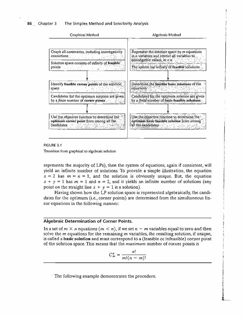
86 Chapter 3 The Simplex Method and Sensitivity Analysis
Graphical Method Algebraic Method
Graph all cOilstniints, inciudiiignoni:i~gativity .restrictions . . :: :.. ' . ...~. .~.' :.;
Solution space consists of infinity ()f fc~ible: ..point.s . ··,,····;·c··:.~
.~~~~iry feasiblecoritef 'poi~t(~tth~~QJ~M~}:;" .. ", .. -":".
Candjdatesfor tl1e optim~m s~hit~(jna're'i~l\iel'lby a finite riumberofconierpoin~s. . ,,;:;'.\;
FIGURE 3.1
Transition from graphical to algebraic solution
~;;t~t~!L*~Btb~r~~n~ ....#¥'~y.~t~!ri..~~i:in~~lti'gt:f~~~i.~~~ ~§IU tl~Il~.::~ •.·
~.~~~~~~~;f.~1~3;~~f·•.~a.si~}hlU.~i~\s,~~)~e ::";
·~;1.~~~~\~~~J~;::t~~~t.~~t}~;lb~~~!~Ie.~,.
~
represents the majority of LPs), then the system of equations, again if consistent, willyield an infinite number of solutions. To provide a simple illustration, the equationx = 2 has m = n = 1, and the solution is obviously unique. But, the equationx + y = 1 has m = 1 and n = 2, and it yields an infinite number of solutions (anypoint on the straight line x + y = 1 is a solution).
Having shown how the LP solution space is represented algebraically, the candidates for the optimum (i.e., corner points) are determined from the simultaneous linear equations in the following manner:
Algebraic Determination of Corner Points.
In a set of m X n equations (m < n), if we set n - m variables equal to zero and thensolve the m equations for the remaining m variables, the resulting solution, if unique,is called a basic solution and must correspond to a (feasible or infeasible) corner pointof the solution space. This means that the maximum number of corner points is
n!en = -----m mIen - m)!
The following example demonstrates the procedure.
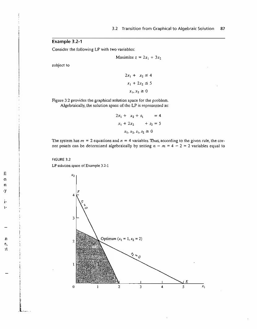
II
ly
3.2 Transition from Graphical to Algebraic Solution 87
Example 3.2-1
Consider the following LP with two variables:
Maximize z = 2Xl + 3xz
subject to
2Xl + Xz $ 4
Xl + 2xz $ 5
Figure 3.2 provides the graphical solution space for the problem.Algebraically, the solution space of the LP is represented as:
2Xt + Xz + Sl = 4
xl + 2xz + Sz = 5
The system has m = 2 equations and n = 4 variables. Thus, according to the given rule, the corner points can be determined algebraically by setting n - m = 4 - 2 = 2 variables equal to
FIGURE 3.2
LP solution space of Example 3.2-1
F4
I
I-
ne,It
3
2
1
o 1 2 3 4 5
E
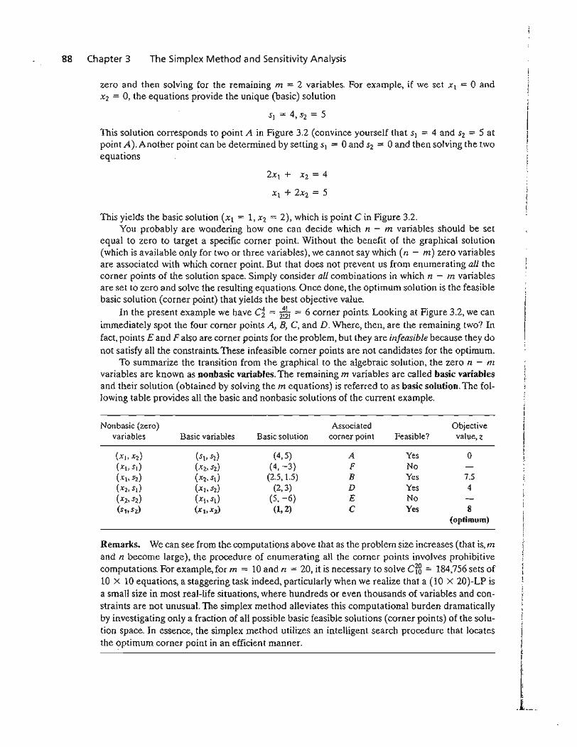
88 Chapter 3 The Simplex Method and Sensitivity Analysis
zero and then solving for the remaining m = 2 variables. For example, if we set Xl = 0 andX2 = 0, the equations provide the unique (basic) solution
sl = 4, s2 = 5
This solution corresponds to point A in Figure 3.2 (convince yourself that s\ = 4 and S2 = 5 atpoint A). Another point can be determined by setting s\ = 0 and S2 = 0 and then solving the twoequations
2x\ + X2 = 4
X\ + 2X2 = 5
This yields the basic solution (Xl = 1, X2 = 2), which is point C in Figure 3.2.You probably are wondering how one can decide which n - m variables should be set
equal to zero to target a specific corner point. Without the benefit of the graphical solution(which is available only for two or three variables), we cannot say which (n - m) zero variablesare associated with which corner point. But that does not prevent us from enumerating all thecorner points of the solution space. Simply consider all combinations in which n - m variablesare set to zero and solve the resulting equations. Once done, the optimum solution is the feasiblebasic solution (corner point) that yields the best objective value.
In the present example we have C~ = 2~~! = 6 corner points. Looking at Figure 3.2, we canimmediately spot the four corner points A, B, C, and D. Where, then, are the remaining two? Infact, points E and F also are corner points for the problem, but they are infeasible because they donot satisfy all the constraints. These infeasible corner points are not candidates for the optimum.
To summarize the transition from the graphical to the algebraic solution, the zero n - mvariables are known as nonbasic variables. The remaining m variables are called basic variablesand their solution (obtained by solving the m equations) is referred to as basic solution. The following table provides all the basic and nonbasic solutions of the current example.
Nonbasic (zero) Associated Objectivevariables Basic variables Basic solution corner point Feasible? value,z
(XI, X2) (Sb 52) (4,5) A Yes 0
(XI> sd (XZ,5Z) (4, -3) F No(x), 52) (X2,5d (2.5,1.5) B Yes 7.5(X2' S\) (Xl, 52) (2,3) D Yes 4(X2, S2) (XI> 5d (5, -6) E No(St, 52) (Xl, Xl) (1,2) C Yes 8
(optimum)
Remarks. We can see from the computations above that as the problem size increases (that is, mand n become large), the procedure of enumerating all the corner points involves prohibitivecomputations. For example, for m = 10 and n = 20, it is necessary to solve ci8 = 184,756 sets of10 X 10 equations, a staggering task indeed, particularly when we realize that a (10 X 20)-LP isa small size in most real-life situations, where hundreds or even thousands of variables and constraints are not unusual. The simplex method alleviates this computational burden dramaticallyby investigating only a fraction of all possible basic feasible solutions (corner points) of the solution space. In essence, the simplex method utilizes an intelligent search procedure that locatesthe optimum corner point in an efficient manner.
i
t)
3.2 Transition from Graphical to Algebraic Solution 89
PROBLEM SET 3.2A
1. Consider the following LP:
Maximize z = 2xI + 3X2
subject to
Xl + 3X2 :5 6
3x[ + 2x2 :5 6
1
S
~
S
~
1
1
)
2.
s
(a) Express the problem in equation form.
(b) Determine all the basic solutions of the problem, and classify them as feasible andinfeasible.
*(c) Use direct substitution in the objective function to determine the optimum basicfeasible solution.
(d) Verify graphically that the solution obtained in (c) is the optimum LP solutionhence, conclude that the optimum solution can be determined algebraically by considering the basic feasible solutions only.
*(e) Show how the infeasible basic solutions are represented on the graphical solutionspace.
Determine the optimum solution for each of the following LPs by enumerating alI thebasic solutions.
(a) Maximize z = 2x[ - 4X2 + 5X3 - 6X4
subject to
Xl + 4X2 - 2X3 + 8X4 :5 2
-xI + 2X2 + 3X3 + 4X4 :5 1
(b) Minimize Z = XI + 2X2 - 3X3 - 2X4
subject to
XI + 2X2 - 3X3 + X4 = 4
XI + 2x2 + X3 + 2x4 = 4
fs
y
s
*3. Show algebraically that all the basic solutions of the following LP are infeasible.
Maximize z = Xl + X2
subject to
XI + 2x2 :5 6
2xI + x2:5 16
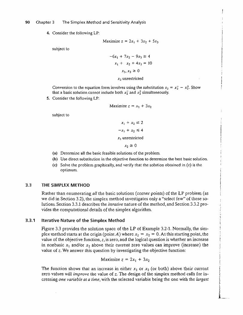
90 Chapter 3 The Simplex Method and Sensitivity Analysis
4. Consider the following LP:
Maximize z = 2xI + 3X2 + 5x3
subject to
-6xI + 7X2 - 9x3 ?:: 4
Xl + X2 + 4x3 = 10
X2 unrestricted
Conversion to the equation form involves using the substitution X2 = xi - x!- Showthat a basic solution cannot include both x2 and xi simultaneously.
5. Consider the following LP:
Maximize z = XI + 3X2
subject to
-XI + x2 s4
Xl unrestricted
X2 ?:: 0
(a) Determine all the basic feasible solutions of the problem.
(b) Use direct substitution in the objective function to determine the best basic solution.
(c) Solve the problem graphically, and verify that the solution obtained in (c) is theoptimum.
3.3 THE SIMPLEX METHOD
Rather than enumerating all the basic solutions (corner points) of the LP problem (aswe did in Section 3.2), the simplex method investigates only a "select few" of these solutions. Section 3.3.1 describes the iterative nature of the method, and Section 3.3.2 provides the computational details of the simplex algorithm.
3.3.1 Iterative Nature of the Simplex Method
Figure 3.3 provides the solution space of the LP of Example 3.2-1. Normally, the simplex method starts at the origin (point A) where Xl = X2 = O. At this starting point, thevalue of the objective function, z, is zero, and the logical question is whether an increasein nonbasic Xl and/or X2 above their current zero values can improve (increase) thevalue of z. We answer this question by investigating the objective function:
Maximize z = 2x1 + 3X2
The function shows that an increase in either Xl or X2 (or both) above their currentzero values will improve the value of z. The design of the simplex method calls for increasing one variable at a time, with the selected variable being the one with the largest
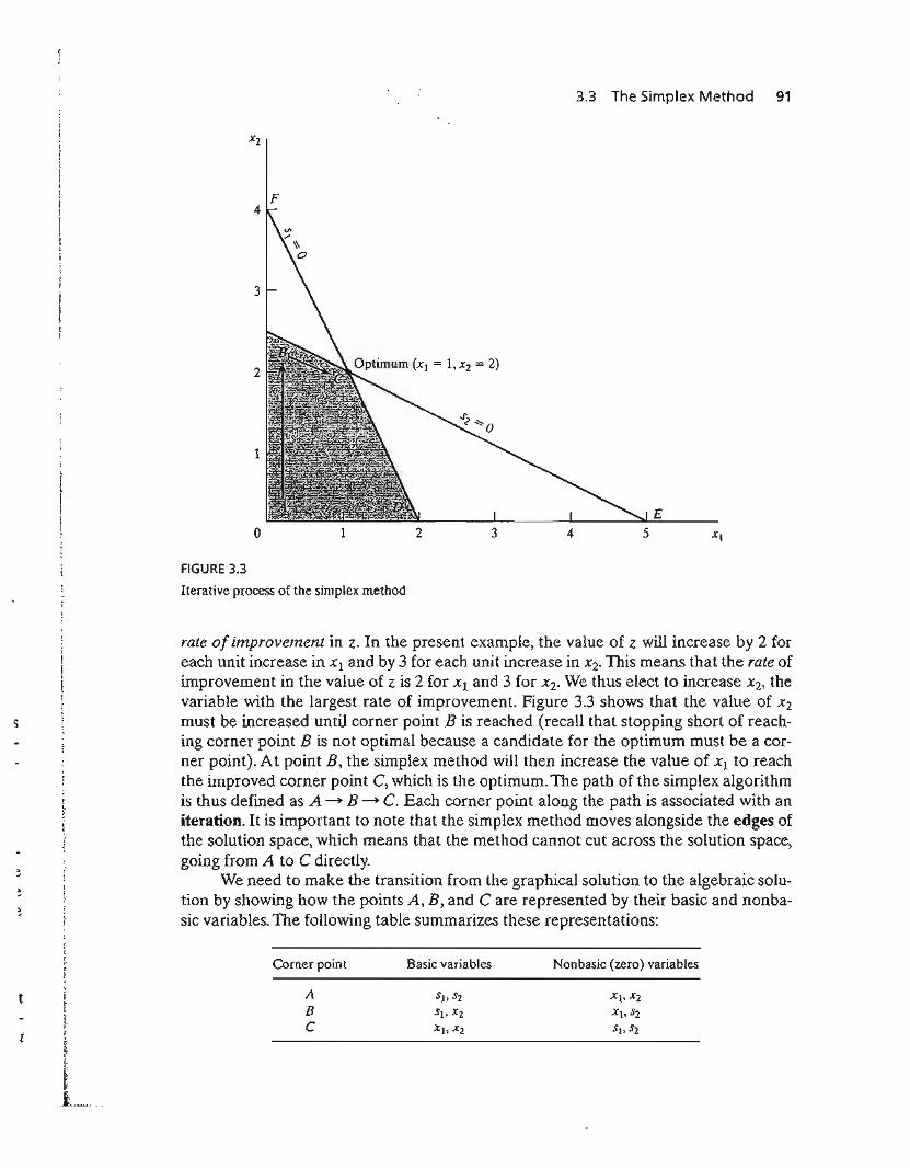
3.3 The Simplex Method 91
F4
E
o 1 2 3 4 5
s
FIGURE 3.3
Iterative process of the simplex method
rate of improvement in z. In the present example, the value of z will increase by 2 foreach unit increase in Xl and by 3 for each unit increase in X2. This means that the rate ofimprovement in the value of z is 2 for Xl and 3 for X2. We thus elect to increase X2, thevariable with the largest rate of improvement. Figure 3.3 shows that the value of X2
must be increased until corner point B is reached (recall that stopping short of reaching corner point B is not optimal because a candidate for the optimum must be a corner point). At point B, the simplex method will then increase the value of Xl to reachthe improved corner point C, which is the optimum. The path of the simplex algorithmis thus defined as A -7 B - C. Each corner point along the path is associated with aniteration. It is important to note that the simplex method moves alongside the edges ofthe solution space, which means that the method cannot cut across the solution space,going from A to C directly.
We need to make the transition from the graphical solution to the algebraic solution by showing how the points A, B, and C are represented by their basic and nonbasic variables. The following table summarizes these representations:
t
Corner point
ABC
Basic variables Nonbasic (zero) variables
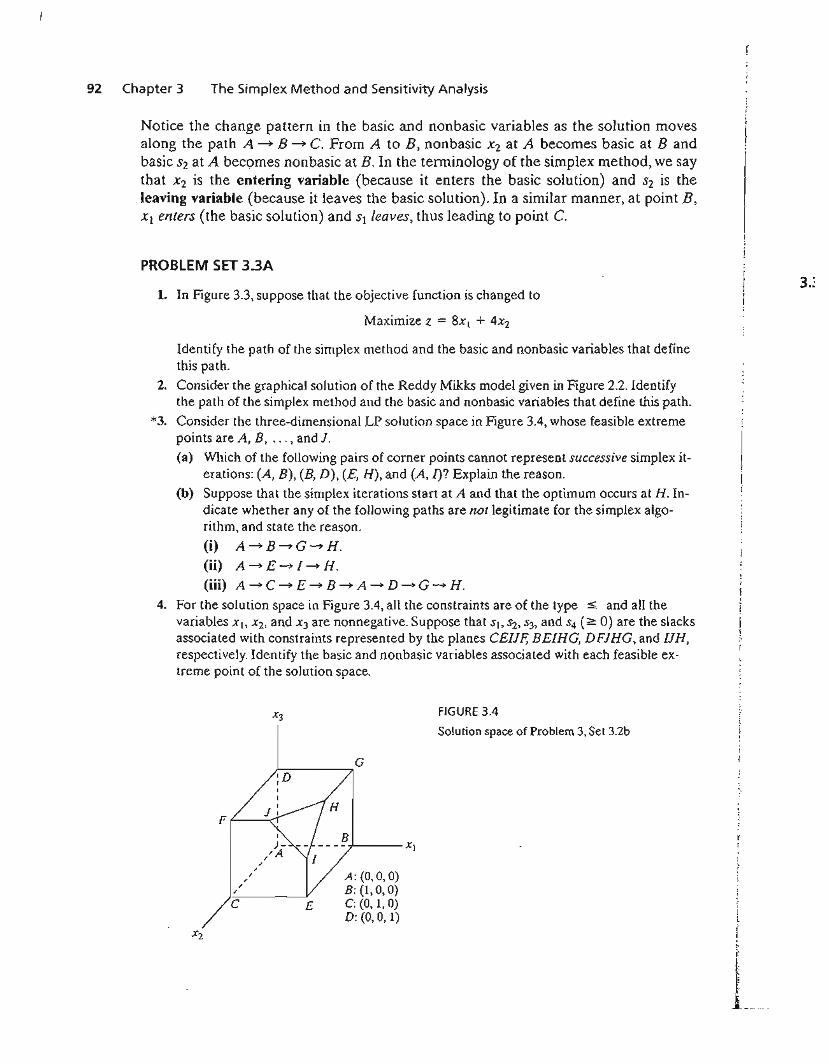
92 Chapter 3 The Simplex Method and Sensitivity Analysis
Notice the change pattern in the basic and nonbasic variables as the solution movesalong the path A ~ B ~ C. From A to B, nonbasic X2 at A becomes basic at Bandbasic S2 at A becomes nonbasic at B. In the terminology of the simplex method, we saythat X2 is the entering variable (because it enters the basic solution) and S2 is theleaving variable (because it leaves the basic solution). In a similar manner, at point B,Xl enters (the basic solution) and Sl leaves, thus leading to point C.
PROBLEM SET 3.3A
1. In Figure 3.3, suppose that the objective function is changed to
Maximize z = 8x[ + 4X2
Identify the path of the simplex method and the basic and nonbasic variables that definethis path.
2. Consider the graphical solution of the Reddy Mikks model given in Figure 2.2. Identifythe path of the simplex method and the basic and nonbasic variables that define this path.
*3. Consider the three-dimensional LP solution space in Figure 3.4, whose feasible extremepoints are A, B, ... , and 1.
(a) Which of the following pairs of corner points cannot represent successive simplex iterations: (A, B), (B, D), (E, H), and (A, I)? Explain the reason.
(b) Suppose that the simplex iterations start at A and that the optimum occurs at H. Indicate whether any of the following paths are not legitimate for the simplex algorithm, and state the reason.
(i) A-B-G-H.
(ii) A-E-I-H.
(iii) A-C-E-B-A-D-G-H.
4. For the solution space in Figure 3.4, all the constraints are of the type :5 and all thevariables XI> X2, and X3 are nonnegative. Suppose that SJ, S2, s3, and S4 (~ 0) are the slacksassociated with constraints represented by the planes CEllF, BEIHG, DFJHG, and IIH,respectively. Identify the basic and nonbasic variables associated with each feasible extreme point of the solution space.
FIGURE 3.4
Solution space of Problem 3, Set 3.2b
G)------"
3.:
F t-----<T
E
-}---Xj
A: (0,0,0)B: (1,0,0)C: (0, 1,0)D: (0,0,1)
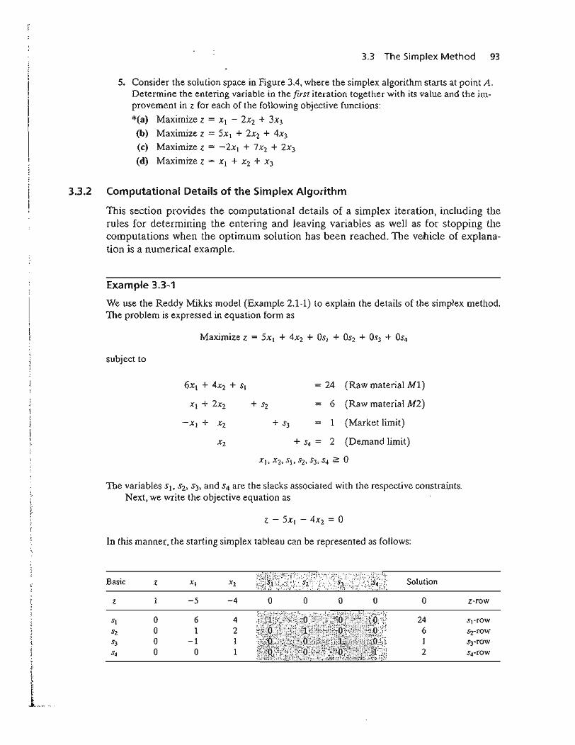
3.3 The Simplex Method 93
5. Consider the solution space in Figure 3.4, where the simplex algorithm starts at point A.Determine the entering variable in the first iteration together with its value and the improvement in z for each of the following objective functions:
*(a) Maximize z = XI - 2X2 + 3X3
(b) Maximize z = 5xI + 2x2 + 4X3
(c) Maximize z = -2XI + 7X2 + 2x3
(d) Maximize z = Xl + X2 + x3
3.3.2 Computational Details of the Simplex Algorithm
This section provides the computational details of a simplex iteration, including therules for determining the entering and leaving variables as well as for stopping thecomputations when the optimum solution has been reached. The vehicle of explanation is a numerical example.
Example 3.3-1
We use the Reddy Mikks model (Example 2.1-1) to explain the details of the simplex method.The problem is expressed in equation form as
subject to
= 24 (Raw material Ml)
6 (Raw material M2)
1 (Market limit)
+ S4 = 2 (Demand limit)
The variables Sb s2, s3, and S4 are the slacks associated with the respective constraints.Next, we write the objective equation as
In this manner, the starting simplex tableau can be represented as follows:
Basic z XI X2
Z 1 -5 -4
St 0 6 4S2 0 1 2S3 0 -1 1S4 0 0 1
o o o o
Solution
o
24612
z-row
St-rowSz-FOW
SrTOW
S4-fOW
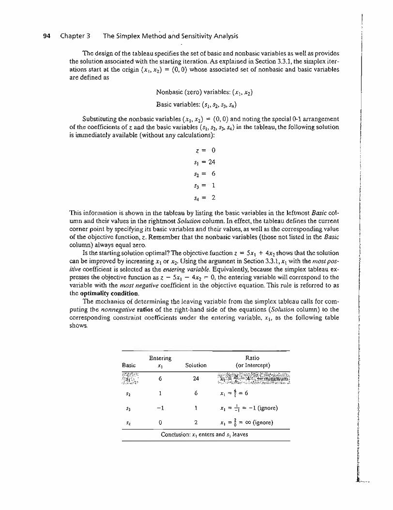
94 Chapter 3 The Simplex Method and Sensitivity Analysis
The design of the tableau specifies the set of basic and nonbasic variables as well as providesthe solution associated with the starting iteration. As explained in Section 3.3.1, the simplex iterations start at the origin (Xl> X2) = (0,0) whose associated set of nonbasic and basic variablesare defined as
Nonbasic (zero) variables: (Xl> X2)
Basic variables: (S1> S2, 53, S4)
Substituting the nonbasic variables (Xl> X2) = (0,0) and noting the special 0-1 arrangementof the coefficients of z and the basic variables (S1> 52, 53,54) in the tableau, the following solutionis immediately available (without any calculations):
z = 0
51 = 24
52 = 6
53 = 1
54 = 2
This information is shown in the tableau by listing the basic variables in the leftmost Basic column and their values in the rightmost Solution column. In effect, the tableau defines the currentcorner point by specifying its basic variables and their values, as well as the corresponding valueof the objective function, z. Remember that the nonbasic variables (those not listed in the Basiccolumn) always equal zero.
Is the starting solution optimal? The objective function z = 5xl + 4xz shows that the solutioncan be improved by increasing Xl or X2' Using the argument in Section 3.3.1, Xl with the most positive coefficient is selected as the entering variable. Equivalently, because the simplex tableau expresses the objective function as z - 5x} - 4xz = 0, the entering variable will correspond to thevariable with the most negative coefficient in the objective equation. This rule is referred to asthe optimality condition.
The mechanics of determining the leaving variable from the simplex tableau calls for computing the nonnegative ratios of the right-hand side of the equations (Solution column) to thecorresponding constraint coefficients under the entering variable, Xl> as the following tableshows.
EnteringBasic Xl Solution
Ratio(or Intercept)
Conclusion: Xl enters and 51 leaves
Sz 1
-1
o
24
6
1
2
Xl = ~ = -1 (ignore)
Xl = ~ = 00 (ignore)
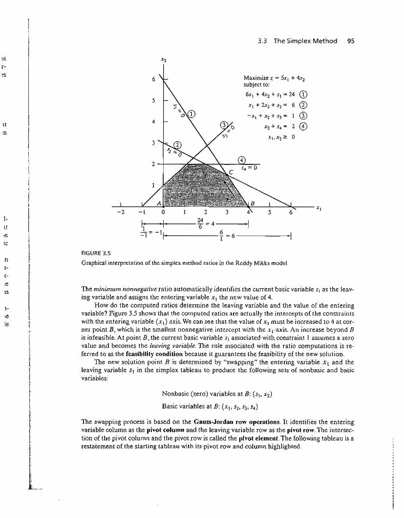
3.3 The Simplex Method 95
r-
,I
Maximize z = 5xI + 4x2subject to:
6xl + 4x2 + 51 = 24 CD®CDo
2-+--....
11' ·1-·-- = -I, 6 - 6 'I-1 ....f-------- 1 - -------~
lItIeic
56Xl + 2x2 + S2 =
-XI + x2 + S3 =It 4
x2 + 54 = 2on
0xl,x2~
~s
onS"
(
IC
IS
1-
Ie
FIGURE 3.5
Graphical interpretation of the simplex method ralios in the Reddy Mikks model
The minimum nonnegative ratio automatically identifies the current basic variable SI as the leaving variable and assigns the entering variable Xl the new value of 4.
How do the computed ratios determine the leaving variable and the value of the enteringvariable? Figure 3.5 shows that the computed ratios are actually the intercepts of the constraintswith the entering variable (Xl) axis. We can see that the value of Xl must be increased to 4 at corner point B, which is the smallest nonnegative intercept with the xl-axis. An increase beyond Bis infeasible. At point B, the current basic variable SI associated with constraint 1 assumes a zerovalue and becomes the leaving variable. The rule associated with the ratio computations is referred to as the feasibility condition because it guarantees the feasibility of the new solution.
The new solution point B is determined by "swapping" the entering variable Xl and theleaving variablesl in the simplex tableau to produce the following sets of nonbasic and basicvariables:
Nonbasic (zero) variables at B: (SI> X2)
Basic variables at B: (Xl> 52, 53, S4)
The swapping process is based on the Gauss-Jordan row operations. It identifies the enteringvariable column as the pivot column and the leaving variable row as the pivot row. The intersection of the pivot \:olumn and the pivot row is called the pivot element. The following tableau is arestatement of the starting tableau with its pivot TOW and column highlighted.
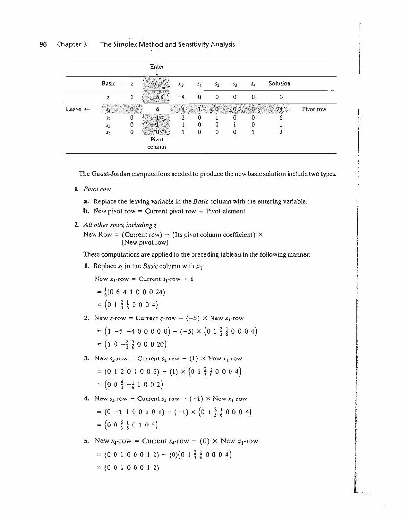
96 Chapter 3 The Simplex Method and Sensitivity Analysis
Enter!
Basic Solution
Leave ~ \?~j~~:~i\~~:~}~;~~~}~~~~\l 6 1j~;~~~~~{~~i:i.::{~:~'{~\~:~.~·~:~;.;f~~~~t~k~i}t~;:Q_~\~l:~~~~g~~Q::t;0.~{f~~1~~~~~;~.;~/:f
:: ~il~~: ~ ~ ! ~ 1Pivot
column
Pivot row
TIle Gauss-Jordan computations needed to produce the new basic solution include two types.
1. Pivot row
a. Replace the leaving variable in the Basic column with the entering variable.
b. New pivot row = Current pivot row + Pivot element
2. All other rows, including z
New Row == (Current row) - (Its pivot column coefficient) X
(New pivot row)
These computations are applied to the preceding tableau in the following manner:
1. Replace Sl in the Basic column with Xl:
New Xl-row == Current sl-row + 6
== ~(O 6 4 1 0 0 0 24)
= (0 1 ~ ~ 0 0 0 4)
2. New z-row == Current z-row - (-5) X New xl-row
== (1 -5 -4 0 0 0 0 0) - (-5) x (0 1 ~ ~ 0 0 0 4)
== (1 0 -~ ~ 0 0 0 20)
3. New srrow == Current S2-row - (1) X New xl-row
== (0 1 2 0 1 0 0 6) - (1) X (0 1 ~ k0 004)
== (0 0 j -k 1 0 0 2)
4. New srrow == Current srrow - (-1) x New Xrrow
== (0 -1 100 1 0 1) - (-1) X (0 1 ~ i 0 0 0 4)==(OO~i0105)
5. New 54-fOW == Current 54-row - (0) x New xrrow
== (0 0 1 0 0 0 1 2) - (0)(0 1 ~ k0 0 0 4)= (0 0 1 0 0 0 1 2)
3.3 The Simplex Method 97
The new basic solution is (x" 52, 53, 54), and the new tableau becomes
Basic
z 1 o o o o
Solution
20
Observe that the new tableau has the same properties as the starting tableau. When we setthe new nonbasic variables X2 and S1 to zero, the Solution column automatically yields the newbasic solution (Xl = 4,52 = 2,53 = 5, S4 = 2). This "conditioning" of the tableau is the resultof the application of the Gauss-Jordan row operations. The corresponding new objectivevalue is z = 20, which is consistent with
New z = Old z + New xl-value X its objective coefficient
= 0 + 4 x 5 = 20
In the last tableau, the optimality condition shows that X2 is the entering variable. The feasibility condition produces the following
Thus, 52 leaves the basic solution and new value of X2 is 1.5. The corresponding increase
in z is ~ Xl = ~ X 1.5 = 1, which yields new z = 20 + 1 = 21.
Replacing 52 in the Basic column with entering X2, the following Gauss-Jordan row operations are applied:
1. New pivot xz-row = Current 5z-row -0- ~
2. New z-row = Current z-row - (-~) x New xz-row
3. New Xl-row = Current XI-row - U) x New xz-row
4. New 53-row = Current STrow - (~) X New xz-row
5. New S4-row = Current S4-row - (1) X New xTrow
4 X2 = 4 -:- ~ = 6
2 ;:I;~;~:E~#;\+};~;;t~JmipXIri~fu)';;5 X2 = 5 -:- ~ = 3
2 X2 := 2 -i- 1 = 2
Solution Ratio
2:34J~3
EnteringX2
Xl
~U~ii:·:::: '.
Basic
98 Chapter 3 The Simplex Method and Sensitivity Analysis
These computations produce the following tableau:
Basic z XI X2 51 52 53 54 Solution
z 1 0 0 3 1 0 0 214" 2
XI 0 1 0 ! 1 0 0 34 -20 0 1 1 ~ 0 0 3
x2 -8 4 20 0 0 3 5 1 0 5
53 8 -4 :2
54 0 0 0 I -~ 0 1 18 4 2
Based on the optimality condition, none of the z-row coefficients associated with the nonbasicvariables, Sl and 52, are negative. Hence, the last tableau is optimal.
TIle optimum solution can be read from the simplex tableau in the following manner. Theoptimal values of the variables in the Basic column are given in the right-hand-side Solution column and can be interpreted as
Decision variable Optimum value
332
21
Recommendation
Produce 3 tons of exterior paint dailyProduce 1.5 tons of interior paint dailyDaily profit is $21,000
You can verify that the values SJ = S2 = 0, S3 = ~,54 = ~ are consistent with the given values ofXl and X2 by substituting out the values of XI and X2 in the constraints.
The solution also gives the status of the resources. A resource is designated as scarce if theactivities (variables) of the model use the resource completely. Otherwise, the resource isabundant. This information is secured from the optimum tableau by checking the value of theslack variable associated with the constraint representing the resource. If the slack value iszero, the resource is used completely and, hence, is classified as scarce. Otherwise, a positiveslack indicates that the resource is abundant. The following table classifies the constraints ofthe model:
Resource Slack value Status
Raw material, Ml 51 = 0 ScarceRaw material, M2 52 = 0 ScarceMarket limit 53 = ~ Abundant
Demand limit 5 - 1 Abundant4 - 2
Remarks. The simplex tableau offers a wealth of additional information that includes:
fr,,i
If
I
1. Sensitivity anaLysis, which deals with determining the conditions that will keep the currentsolution unchanged.
2. Post-optimal analysis, which deals with finding a new optimal solution when the data of.the model are changed. t
1it
L
eis
3.3.3
3.3 The Simpl~x Method 99
Section 3.6 deals with sensitivity analysis. The more involved topic of post-optimal analysisis covered in Chapter 4.
TORA Moment.
The Gauss-Jordan computations are tedious, voluminous, and, above aU, boring. Yet,they are the least important, because in practice these computations are carried out bythe computer. What is important is that you understand how the simplex methodworks. TORA's interactive user-guided option (with instant feedback) can be of help inthis regard because it allows you to decide the course of the computations in the simplex method without the burden of carrying out the Gauss-Jordan calculations. Touse TORA with the Reddy Mikks problem, enter the model and then, from theSOLVEIMODIFY menu, select Solve~ Algebraic => Iterations~ AIl::SliiCk. (TheAll-Slack selection indicates that the starting basic solution consists of slack variablesonly. The remaining options will be presented in Sections 3.4,4.3, and 7.4.2.) Next, click:~(r:r~LQ!i~P4fS.cte~il; You can generate one or aU iterations by clicking Next Iteia:tibn:or AllIterations. If you opt to generate the iterations one at a time, you can interactively specify the entering and leaving variables by clicking the headings of their corresponding column and row. If your selections are correct, the column turns green andthe row turns red. Else, an error message will be posted.
Summary of the Simplex Method
So far we have dealt with the maximization case. In mlrnmlZation problems, theoptimality condition calls for selecting the entering variable as the nonbasic variable withthe most positive objective coefficient in the objective equation, the exact opposite ruleof the maximization case. This follows because max z is equivalent to min (-z). As forthe feasibility condition for selecting the leaving variable, the rule remains unchanged.
Optimality condition. The entering variable in a maximization (minimization)problem is the nonbasic variable having the most negative (positive) coefficient in thez-row. Ties are broken arbitrarily. The optimum is reached at the iteration where all thez-row coefficients of the nonbasic variables are nonnegative (nonpositive).
Feasibility condition. For both the maximization and the minimization problems,the leaving variable is the basic variable associated with the smallest nonnegative ratio(with strictly positive denominator). Ties are broken arbitrarily.
Gauss-Jordan row operations.
1. Pivot row
a. Replace the leaving variable in the Basic column with the entering variable.nt b. New pivot row = Current pivot row -+- Pivot element
of
L
2. All other rows, including zNew row = (Current row) - (pivot column coefficient) X (New pivot row)
100 Chapter 3 The Simplex Method and Sensitivity Analysis
The steps of the simplex method are
Step 1.Step 2.
Step 3.Step 4.
Determine a starting basic feasible solution.Select an entering variable using the optimality condition. Stop if there is noentering variable; the last solution is optimal. Else, go to step 3.Select a leaving variabLe using the feasibility condition.Determine the new basic solution by using the appropriate Gauss-Jordancomputations. Go to step 2.
PROBLEM SET 3.3B
1. This problem is designed to reinforce your understanding of the simplex feasibility condition. In the first tableau in Example 3.3-1, we used the minimum (nonnegative) ratio testto determine the leaving variable. Such a condition guarantees that none of the new values of the basic variables will become negative (as stipulated by the definition of the LP).To demonstrate this point, force 52, instead of 5b to leave the basic solution. Now, look atthe resulting simplex tableau, and you will note that 51 assumes a negative value (= -12),meaning that the new solution is infeasible. This situation will never occur if we employthe minimum-ratio feasibility condition.
2. Consider the following set of constraints:
Xl + 2X2 + 2X3 + 4X4 :5 40
2x1 - x2 + X3 + 2X4 :5 8
4x1 - 2X2 + X3 - X4:5 10
Solve the problem for each of the following objective functions.
(a) Maximize z = 2Xl + X2 - 3X3 + 5X4'
(b) Maximize z = 8Xl + 6X2 + 3X3 - 2X4'
(c) Maximize z = 3x1 - X2 + 3X3 + 4X4'
(d) Minimize z = 5xI - 4x2 + 6X3 - 8X4'
*3. Consider the following system of equations:
Xl + 2X2 - 3X3 + 5X4 + Xs =4
=8
=3
+ Xs = 0
Let xs, x6,' .. , and Xg be a given initial basic feasible solution. Suppose that Xl becomesbasic. Which of the given basic variables must become nonbasic at zero level to guaranteethat all the variables remain nonnegative, and what is the value of Xl in the new solution?Repeat this procedure for x2, x3, and X4'
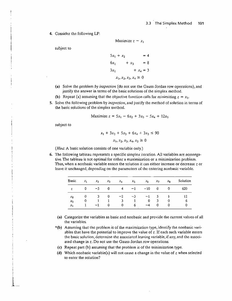
3.3 The Simplex Method 101
4. Consider the following LP:
Maximize z = Xl
subject to
=4
=8
(a) Solve the problem by inspection (do not use the Gauss-Jordan row operations), andjustify the answer in terms of the basic solutions of the simplex method.
(b) Repeat (a) assuming that the objective function calls for minimizing z = Xl.
5. Solve the following problem by inspection, and justify the method of solution in terms ofthe basic solutions of the simplex method.
Maximize z = 5x] - 6X2 + 3X3 - 5X4 + 12xs
subject to
(Hint: A basic solution consists of one variable only.)
6. The following tableau represents a specific simplex iteration. All variables are nonnegative. The tableau is not optimal for either a maximization or a minimization problem.ll1Us, when a nonbasic variable enters the solution it can either increase or decrease z orleave it unchanged, depending on the parameters of the entering nonbasic variable.
Basic Xl X2 X3 X4 X5 X6 X7 Xg Solution
z 0 -5 0 4 -1 -10 0 0 620
Xa 0 3 0 -2 -3 -1 5 1 12X3 0 1 1 3 1 0 3 0 6XI 1 -1 0 0 6 -4 0 0 0
(a) Categorize the variables as basic and nonbasic and provide the current values of allthe variables.
*(b) Assuming that the problem is of the maximization type, identify the nonbasic variables that have the potential to improve the value of z. If each such variable entersthe basic solution, determine the associated leaving variable, if any, and the associated change in z. Do not use the Gauss-Jordan row operations.
(c) Repeat part (b) assuming that the problem is of the minimization type.
(d) Which nonbasic variable(s) will not cause a change in the value of Z when selectedto enter the solution?
f.J. __
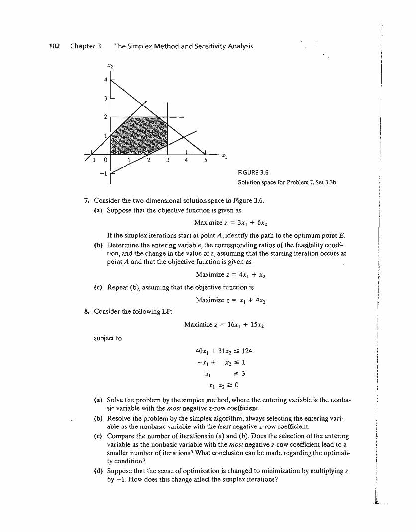
102 Chapter 3 The Simplex Method and Sensitivity Analysis
FIGURE 3.6
Solution space for Problem 7, Set 3.3b
7. Consider the two-dimensional solution space in Figure 3.6.(3) Suppose that the objective function is given as
Maximize z = 3XI + 6x2
If the simplex iterations start at point A, identify the path to the optimum point E.
(b) Determine the entering variable, the corresponding ratios of the feasibility condition, and the change in the value of z, assuming that the starting iteration occurs atpoint A and that the objective function is given as
Maximize z = 4XI + X2
(c) Repeat (b), assuming that the objective function is
Maximize z = Xl + 4X2
8. Consider the following LP:
Maximize z = 16xI + 15x2
subject to
40XI + 31x2 :5 124
-xl + X2:5 1
Xl :5 3
XI> X2 ;::: 0
(a) Solve the problem by the simplex method, where the entering variable is the nonbasic variable with the most negative z-row coefficient.
(b) Resolve the problem by the simplex algorithm, always selecting the entering variable as the nonbasic variable with the least negative z-row coefficient.
(c) Compare the number of iterations in (a) and (b). Does the selection of the enteringvariable as the nonbasic variable with the most negative z-row coefficient lead to asmaller number of iterations? What conclusion can be made regarding the optimality condition?
(d) Suppose that the sense of optimization is changed to minimization by multiplying zby -1. How does this change affect the simplex iterations?
rr
I[
lI·
f!~
1.....
3.4 Artificial Starting Solution 103
*9. In Example 3.3-1, show how the second best optima) value of z can be determined fromthe optimal tableau.
10. Can you extend the procedure in Problem 9 to determine the third best optimal value. of z?1L The Gutchi Company manufactures purses, shaving bags, and backpacks. The construction
includes leather and synthetics, leather being the scarce raw material. The productionprocess requires two types of skilled labor: sewing and finishing. The following table givesthe availability of the resources, their usage by the three products, and the profits per unit.
Resource requirements per unit
Resource Purse Bag Backpack Daily availability
Leather (ft2) 2 1 3 42 ft2Sewing (hr) 2 1 2 40 hrFinishing (hr) 1 .5 1 4S hr
Selling price ($) 24 22 45
(a) Formulate the problem as a linear program and find the optimum solution (usingTORA, Excel Solver, or AMPL).
(b) From the optimum solution determine the status of each resource.
12. TORA experiment. Consider the following LP:
Maximize z = XI + X2 + 3X3 + 2X4
subject to
1-
1-
lI,
fif,
1.....
2Xj + 3X2 - 2x3 + 3X4 :s; 3
- XI + xJ + 2X4 :s; 0
(a) Use TORA's iterations option to determine the optimum tableau.
(b) Select any nonbasic variable to "enter" the basic solution, and click Next Iteration toproduce the associated iteration. How does the new objective value compare withthe optimum in (a)? The idea is to show that the tableau in (a) is optimum becausenone of the nonbasic variables can improve the objective value.
13. TORA experiment. In Problem 12, use TORA to find the next-best optimal solution.
3.4 ARTIFICIAL STARTING SOLUTION
As demonstrated in Example 3.3-1, LPs in which all the constraints are (::5) with nonnegative right-hand sides offer a convenient all-slack starting basic feasible solution.Models involving ( =) and/or (» constraints do not.
The procedure for starting "ill-behaved" LPs with (=) and (:;:::) constraints is touse artificial variables that play the role of slacks at the first iteration, and then disposeof them legitimately at a later iteration. Two closely related methods are introducedhere: the M-method and the two-phase method.
104 Chapter 3
3.4.1 M-Method
The Simplex Method and Sensitivity Analysis
The M-method starts with the LP in equation form (Section 3.1). If equation i does nothave a slack (or a variable that can play the role of a slack), an artificial variable, Ri , isadded to form a starting solution similar to the convenient all-slack basic solution.However, because the artificial variables are not part of the original LP model, they areassigned a very high penalty in the objective function, thus forcing them (eventually) toequal zero in the optimum solution. This will always be the case if the problem has afeasible solution. The following rule shows how the penalty is assigned in the cases ofmaximization and minimization:
Penalty Rule for Artificial Variables.
Given M, a sufficiently large positive value (mathematically, M - 00), the objective coefficient of an artificial variable represents an appropriate penalty if:
. . . .. . . { - M, in maximization problemsArtifiCial vanable objective coefficient = .. . .. I
M, 10 mlmmlzatlOn prob ems
Example 3.4-1
Minimize z = 4Xt + X2
subject to
3x\ + X2 = 3
4XI + 3x2 ;;:: 6
Xt + 2X2 :5 4
Using X3 as a surplus in the second constraint and X4 as a slack in the third constraint, theequation form of the problem is given as
Minimize z = 4xt + X2
subject to
3x\ + X2 = 3
4Xl + 3x2 - X3 = 6
The third equation has its slack variable, X4, but the first and second equations do not. Thus,we add the artificial variables R\ and R2 in the first two equations and penalize them in the objective function with M R1 + MRz (because we are minimizing). The resulting LP is given as
Minimize z = 4xl + Xz + MR1 + MRz
~I:1
t,.~,
ff:f.I
!~
L
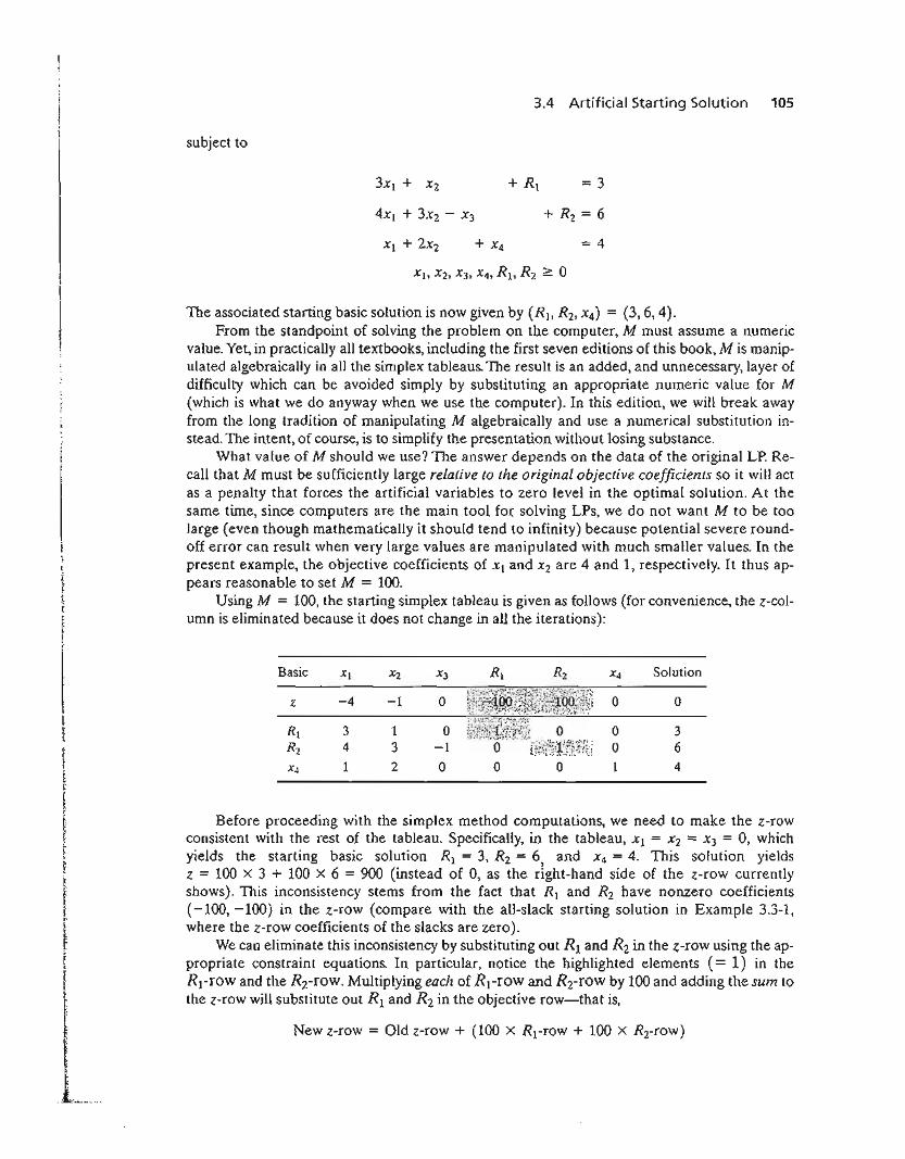
3.4 Artificial Starting Solution 105
subject to
=3
+ Rz = 6
=4
The associated starting basic solution is now given by (RJ, R2, X4) = (3,6,4).From the standpoint of solving the problem on the computer, M must assume a numeric
value. Yet, in practically all textbooks, including the first seven editions of this book, M is manipulated algebraically in all the simplex tableaus. The result is an added, and unnecessary, layer ofdifficulty which can be avoided simply by substituting an appropriate numeric value for M(which is what we do anyway when we use the computer). In this edition, we will break awayfrom the long tradition of manipulating M algebraically and use a numerical substitution instead. The intent, of course, is to simplify the presentation without losing substance.
What value of M should we use? The answer depends on the data of the original LP. Recall that M must be sufficiently large relative to the original objective coefficients so it will actas a penalty that forces the artificial variables to zero level in the optimal solution. At thesame time, since computers are the main tool for solving LPs, we do not want M to be toolarge (even though mathematically it should tend to infinity) because potential severe roundoff error can result when very large values are manipulated with much smaller values. In thepresent example, the objective coefficients of Xl and X2 are 4 and 1, respectively. It thus appears reasonable to set M = 100.
Using M = 100, the starting simplex tableau is given as follows (for convenience, the z-column is eliminated because it does not change in all the iterations):
Basic XI X2 X3 R[ R2 X4 Solution
z -4 -1 0 ~1m~i~Mj~H.i~W~8~:;~~j 0 0
R[ 3 1 0 fiNiH~~l;iH~t,B 0 0 3R2 4 3 -1 0 ffi:~t:~0~~:f~ffN;'i 0 6
X4 1 2 0 0 0 1 4
Before proceeding with the simplex method computations, we need to make the z-rowconsistent with the rest of the tableau. Specifically, in the tableau, Xl = X2 = X3 = 0, whichyields the starting basic solution R1 = 3, R2 = 6 and X4 = 4. This solution yields,z = 100 X 3 + 100 X 6 = 900 (instead of 0, as the right-hand side of the z-row currentlyshows). This inconsistency stems from the fact that R1 and R2 have nonzero coefficients(-100, -100) in the z-row (compare with the all-slack starting solution in Example 3.3-1,where the z-row coefficients of the slacks are zero).
We can eliminate this inconsistency by substituting out R1 and R2 in the z-row using the appropriate constraint equations. In particular, notice the highlighted elements (= 1) in theR1-row and the Rrrow. Multiplying each of R1-row and R2-row by 100 and adding the sum tothe z-row will substitute out R1 and R2 in the objective row-that is,
New z-row = Old z-row + (100 X Rrrow + 100 X R2-row)
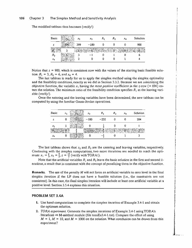
106 Chapter 3 The Simplex Method and Sensitivity Analysis
The modified tableau thus becomes (verify!)
-100 o o o
Solution
900
Notice that z = 900, which is consistent now with the values of the starting basic feasible solution: RI = 3, Rz = 6, and X4 = 4.
The last tableau is ready for us to apply the simplex method using the simplex optimalityand the feasibility conditions, exactly as we did in Section 3.3.2. Because we are minimizing theobjective function, the variable Xl having the most positive coefficient in the z-row (= 696) enters the solution. The minimum ratio of the feasibility condition specifies R 1 as the leaving variable (verify!).
Once the entering and the leaving variables have been determined, the new tableau can becomputed by using the familiar Gauss-Jordan operations.
Basic Xl ~it¥~t~J4w1~ X3 R1 Rz X4 Solution
z 0 ~1~~~~~,~w.~~~ -100 -232 0 0 204
The last tableau shows that Xz and Rz are the entering and leaving variables, respectively.Continuing with the simplex computations, two more iterations are needed to reach the opti-
. - ~ - 2 -.!.z ( of . hTORAI)mum. Xl - 5' Xz - 5' Z - 5 ven y WIt ..Note that the artificial variables R1 and Rzleave the basic solution in the first and second it
erations, a result that is consistent with the concept of penalizing them in the objective function.
Remarks. The use of the penalty M will not force an artificial variable to zero level in the finalsimplex iteration if the LP does not have a feasible solution (i.e., the constraints are notconsistent). In this case, the final simplex iteration will include at least one artificial variable at apositive level. Section 3.5.4 explains this situation.
PROBLEM SET 3.4A
1. Use hand computations to complete the simplex iteration of Example 3.4-1 and obtainthe optimum solution.
2. TORA experiment. Generate the simplex iterations of Example 3.4-1 using TORA's.iterations => M-fuethbd module (file toraEx3.4-l.txt). Compare the effect of usingM = 1, M == 10, and M = 1000 on the solution. What conclusion can be drawn from thisexperiment?
t
L
3.4 Artificial Starting Solution 107
3. In Example 3.4-1, identify the starting tableau for each of the following (independent)cases, and develop the associated z-row after substituting out all the artificial variables:
*(a) The third constraint is Xl + 2X2 ;::: 4.
*(b) The second constraint is 4XI + 3X2 :::::: 6.
(c) The second constraint is 4XI + 3X2 = 6.
(d) The objective function is to maximize z = 4xI + x2'
4. Consider the following set of constraints:
-2XI + 3X2 = 3 (1)
4Xl + 5X2 ;::: 10 (2)
Xl + 2X2:::::: 5 (3)
6Xl+7x2~3 (4)
4XI + 8X2 ;::: 5 (5)
Xl + X2 + X3 = 4
Xl + 4x2 + X4 = 8
Solve the problem for each of the following objective functions:
(a) Maximize z = 2Xl + 3X2 - 5X3'
(b) Minimize z = 2XI + 3X2 - 5x3-
(c) Maximize z = Xl + 2X2 + X3-
(d) Minimize z = 4Xl - 8X2 + 3x3'
Consider the problem
subject to
For each of the following problems, develop the z-row after substituting out the artificialvariables:
(a) Maximize z = 5xI + 6X2 subject to (1), (3), and (4).
(b) Maximizez = 2XI - 7x2subject to (1),(2), (4), and (5).
(c) Minimize z = 3Xl + 6X2 subject to (3), (4), and (5).
(d) Minimize z = 4Xl + 6X2 subject to (1), (2), and (5).
(e) Minimize z = 3XI + 2X2 subject to (1) and (5).
Consider the following set of constraints:
Xl + X2 + x 3 = 7
2x1 - 5x2 + xJ ;::: 10
5.f;:!f~
I,•fr;
r•~
f. *6.I'[
~~"~~
~f:~~
The problem shows that X3 and X4 can play the role of slacks for the two equations. Theydiffer from slacks in that they have nonzero coefficients in the objective function. We canuse X3 and X4 as starting variable, but, as in the case of artificial variables, they must besubstituted out in the objective function before the simplex iterations are carried out.Solve the problem with X3 and X4 as the starting basic variables and without using anyartificial variables.
108 Chapter 3 The Simplex Method and Sensitivity Analysis
7. Solve the following problem using X3 and X4 as starting basic feasible variables. As inProblem 6, do not use any artificial variables.
Minimize z = 3xI + 2X2 + 3X3
subject to
XI + 4X2 + X3 ~ 7
2x1 + X2 + X4 ~ 10
Xl> x2, x3, X4 ~ 0
8. Consider the problem
Maximize z = Xl + 5X2 + 3X3
subject to
Xl + 2X2 + X3 = 3
2Xi - X2 = 4
The variable X3 plays the role of a slack. Thus, no artificial variable is needed in the firstconstraint. However, in the second constraint, an artificial variable is needed. Use thisstarting solution (i.e., X3 in the first constraint and R2 in the second constraint) to solvethis problem.
9. Show how the M-method will indicate that the following problem has no feasible solution.
Maximize z = 2x1 + 5X2
subject to
3XI + 2x2 ~ 6
2x1 + x2:5 2
XI> X2 ~ 0
3.4.2 Two-Phase Method
In the M-method, the use of the penalty M, which by definition must be large relative. to the actual objective coefficients of the model, can result in roundoff error that mayimpair the accuracy of the simplex calculations. The two-phase method alleviates thisdifficulty by eliminating the constant M altogether. As the name suggests, the methodsolves the LP in two phases: Phase I attempts to find a starting basic feasible solution,and, if one is found, Phase II is invoked to solve the original problem.
Summary of the Two-Phase Method
Phase I. Put the problem in equation form, and add the necessary artificial variables to the constraints (exactly as in the M-method) to secure a startingbasic solution. Next, find a basic solution of the resulting equations that,regardless of whether the LP is maximization or minimization, alwaysminimizes the sum of the artificial variables. If the minimum value of the
!fI.,.~
tfri,.
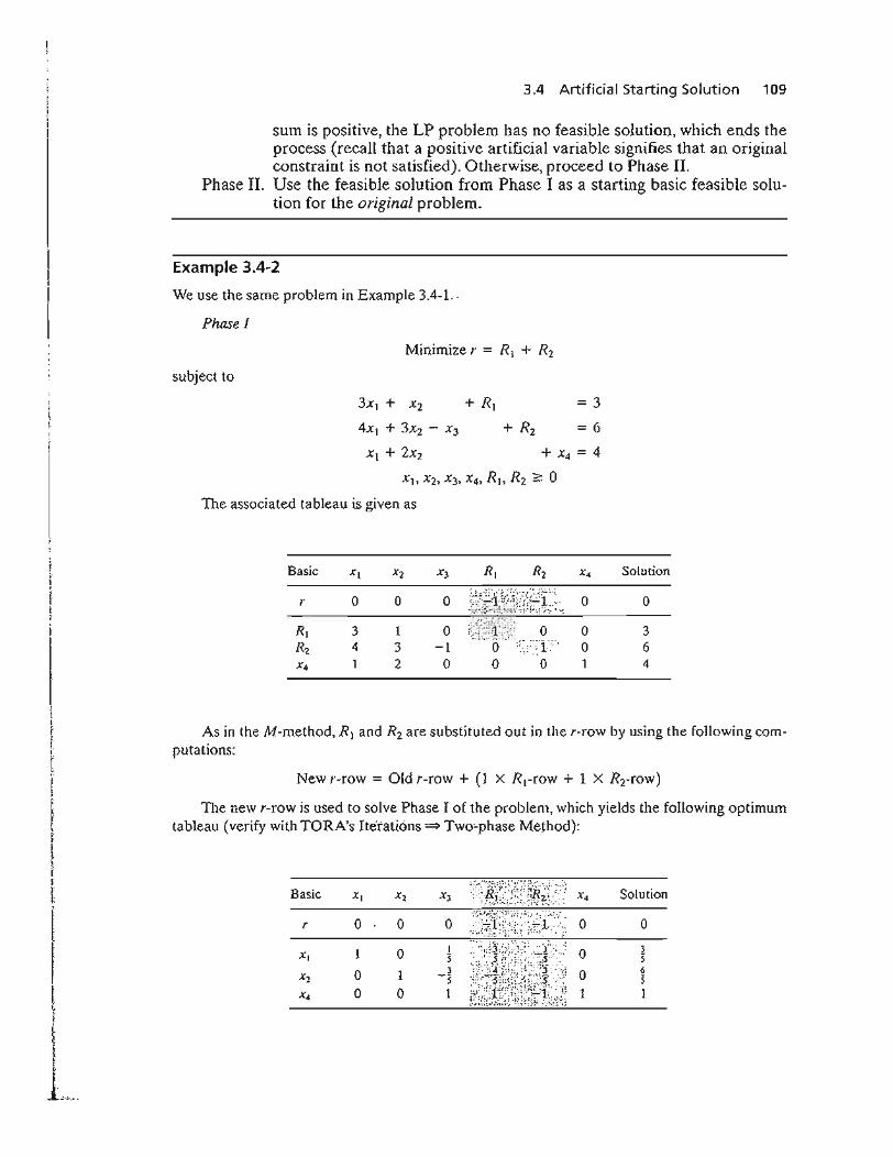
3.4 Artificial Starting Solution 109
sum is positive, the LP problem has no feasible solution, which ends theprocess (recall that a positive artificial variable signifies that an originalconstraint is not satisfied). Otherwise, proceed to Phase II.
Phase II. Use the feasible solution from Phase I as a starting basic feasible solution for the original problem.
Example 3.4-2
We use the same problem in Example 3.4-1..
Phase I
Minimize r = R, + R2
subject to
3x\ + X2 + R, = 3
4x, + 3X2 - X3 + R2 = 6
x, + 2X2 + X4 = 4
The associated tableau is given as
Basic Xl X2 Xl R l R2 X4 Solution
r 0 0 0 e;S:~,~:di::rHti~::·;;; 0 0
R1 3 1 0 :;::;:j:j1Y~(: 0 0 3R2 4 3 - 1 0 "'T: 0 6X4 1 2 0 0 0 1 4
As in the M-method, R( and R2 are substituted out in the r-row by using the following computations:
New r-row = Old r-row + (l X R,-row + 1 x RTrow)
TIle new r-row is used to solve Phase I of the problem, which yields the following optimumtableau (verify with TORA's Iterations => Two~phase Method):
Basic XI
r 0
XI 1
X2 0
X4 0
o
o1
o
o
Solution
o3:56:51
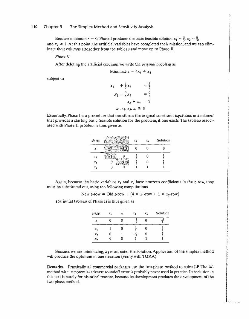
110 Chapter 3 The Simplex Method and Sensitivity Analysis
Because minimum r ;:;: 0, Phase I produces the basic feasible solution Xl = ~, X2 = ~,
and X4 = 1. At this point, the artificial variables have completed their mission, and we can eliminate their columns altogether from the tableau and move on to Phase II.
Phase II
After deleting the artificial columns, we write the original problem as
Minimize z = 4Xl + X2
subject to1+ SX3
3X2 - "5 X3
3"56= 5
Essentially, Phase I is a procedure that transforms the original constraint equations in a mannerthat provides a starting basic feasible solution for the problem, if one exists. The tableau associated with Phase II problem is thus given as
Basic ~i;~il~~tlfki X3 X4 Solution
z ~~~{{~~\tl~§ 0 0 0
~~~{i~~!I 0 3
Xl 5 53 0 6
X2 -s SX4 0 0 1 1 1
Again, because the basic variables Xl and Xz have nonzero coefficients in the z-row, theymust be substituted out, using the following computations.
New z-row = Old z-row + (4 X xrrow + 1 X xz-row)
The initial tableau of Phase II is thus given as
Basic Xl X2 X3 X4 Solution
0 0 1 0 18Z 5 5
1 0 1 0 3XI 5 5
0 1 3 0 6X2 -5 SX4 0 0 1 1 1
Because we are minimizing, x3 must enter the solution. Application of the simplex methodwill produce the optimum in one iteration (verify with TORA).
Remarks. Practically all commercial packages use the two-phase method to solve LP. The Mmethod with its potential adverse roundoff error is probably never used in practice. Its inclusion inthis text is purely for historical reasons, because its development predates the development of thetwo-phase method.
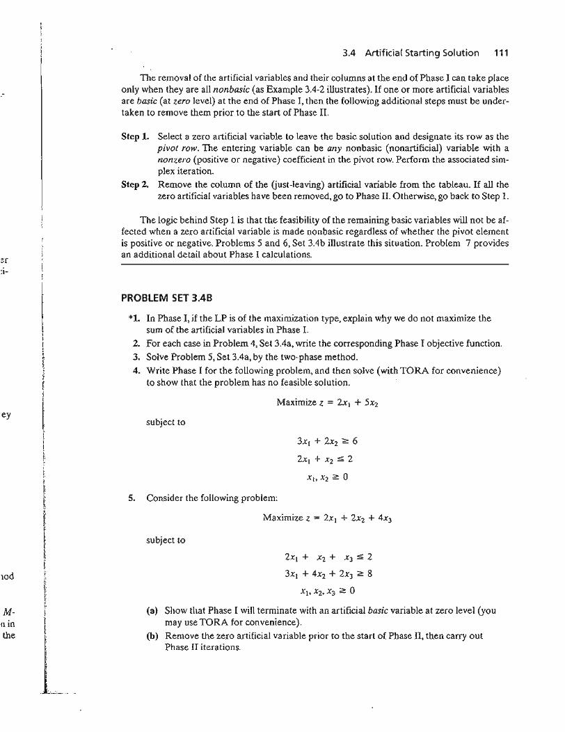
~r
ey
lOd
Mointhe
3.4 Artificial Starting Solution 111
The removal of the artificial variables and their columns at the end of Phase I can take placeonly when they are all nonbasic (as Example 3.4-2 illustrates). If one or more artificial variablesare basic (at zero level) at the end of Phase I, then the following additional steps must be undertaken to remove them prior to the start of Phase II.
Step 1. Select a zero artificial variable to leave the basic solution and designate its row as thepivot row. The entering variable can be any nonbasic (nonartificiaI) variable with anonzero (positive or negative) coefficient in the pivot row. Perform the associated simplex iteration.
Step 2. Remove the column of the (just-leaving) artificial variable from the tableau. If all thezero artificial variables have been removed, go to Phase II. Otherwise, go back to Step 1.
The logic behind Step 1 is that the feasibility of the remaining basic variables will not be affected when a zero artificial variable is made nonbasic regardless of whether the pivot elementis positive or negative. Problems 5 and 6, Set 3Ab illustrate this situation. Problem 7 providesan additional detail about Phase I calculations.
PROBLEM SET 3.4B
*1. In Phase I, if the LP is of the maximization type, explain why we do not maximize thesum of the artificial variables in Phase I.
2. For each case in Problem 4, Set 3.4a, write the corresponding Phase I objective function.
3. Solve Problem 5, Set 3.4a, by the two-phase method.
4. Write Phase I for the following problem, and then solve (with TORA for convenience)to show that the problem has no feasible solution.
Maximize z = 2Xl + 5X2
subject to
5. Consider the following problem:
Maximize z = 2xl + 2x2 + 4x3
subject to
2Xl + X2 + X3:5 2
3xl + 4X2 + 2x3 ~ 8
(a) Show that Phase I will terminate with an artificial basic variable at zero level (youmay use TORA for convenience).
(b) Remove the zero artificial variable prior to the start of Phase II, then carry outPhase II iterations.
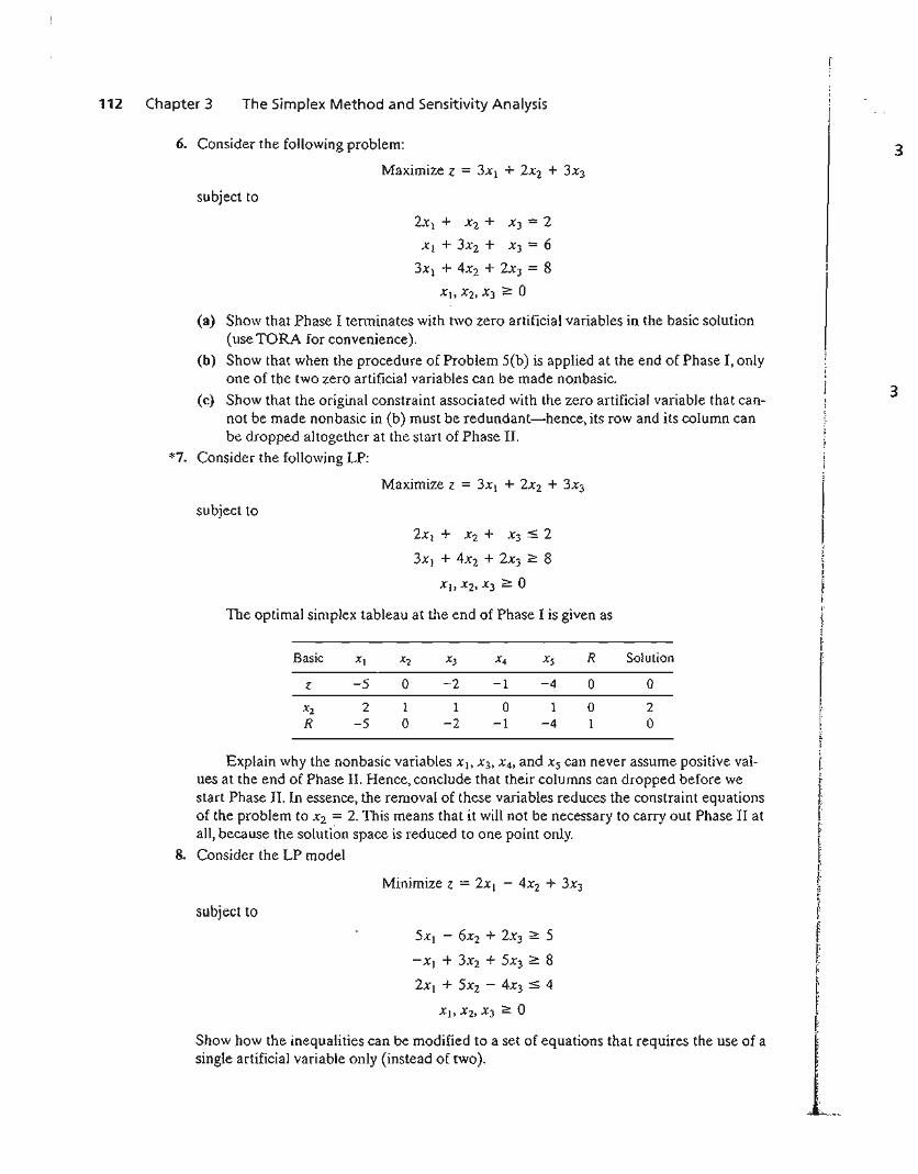
112 Chapter 3 The Simplex Method and Sensitivity Analysis
6. Consider the following problem:
Maximize z = 3Xl + 2X2 + 3X3
subject to
2Xl + X2 + X3 = 2
Xl + 3X2 + X3 = 6
3Xl + 4X2 + 2x3 = 8
Xl> X2, X3 2: 0
(a) Show that Phase I terminates with two zero artificial variables in the basic solution(useTORA for convenience).
(b) Show that when the procedure of Problem 5(b) is applied at the end of Phase I, onlyone of the two zero artificial variables can be made nonbasic.
(c) Show that the original constraint associated with the zero artificial variable that cannot be made nonbasic in (b) must be redundant-hence, its row and its column canbe dropped altogether at the start of Phase II.
*7. Consider the following LP:
Maximize z = 3x\ + 2x2 + 3X3
subject to
2x\ + X2 + x3:5 2
3x] + 4X2 + 2X3 2: 8
The optimal simplex tableau at the end of Phase I is given as
Basic Xl X2 X3 X4 Xs R Solution
Z -5 0 -2 -1 -4 0 0
X 2 2 1 1 0 1 0 2R -5 0 -2 -1 -4 1 0
Explain why the nonbasic variables Xl> X3, X4, and Xs can never assume positive values at the end of Phase II. Hence, conclude that their columns can dropped before westart Phase II. In essence, the removal of these variables reduces the constraint equationsof the problem to X2 = 2. This means that it will not be necessary to carry out Phase II atall, because the solution space is reduced to one point only.
8. Consider the LP model
Minimize z = 2Xl - 4X2 + 3x3
subject to
5x\ - 6X2 + 2X3 2: 5
- Xl + 3X2 + 5x3 2: 8
2Xl + 5X2 - 4x3 :5 4
Show how the inequalities can be modified to a set of equations that requires the use of asingle artificial variable only (instead of two).
3
3
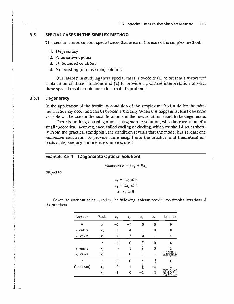
3.5 Special Cases in the Simplex Method 113
3.5 SPECIAL CASES IN THE SIMPLEX METHOD
This section considers four special cases that arise in the use of the simplex method.
1. Degeneracy2. Alternative optima3. Unbounded solutions4. Nonexisting (or infeasible) solutions
Our interest in studying these special cases is twofold: (1) to present a theoreticalexplanation of these situations and (2) to provide a practical interpretation of whatthese special results could mean in a real-life problem.
3.5.1 Degeneracy
In the application of the feasibility condition of the simplex method, a tie for the minimum ratio may occur and can be broken arbitrarily. When this happens, at least one basicvariable will be zero in the next iteration and the new solution is said to be degenerate.
There is nothing alarming about a degenerate solution, with the exception of asmall theoretical inconvenience, called cycling or circling, which we shall discuss shortly. From the practical standpoint, the condition reveals that the model has at least oneredundant constraint. To provide more insight into the practical and theoretical impacts of degeneracy, a numeric example is used.
Example 3.5-1 (Degenerate Optimal Solution)
Maximize z = 3Xl + 9X2
subject to
Xl + 4X2 5 8
Xl + 2X2 :5 4
xl> X2 ~ 0
Given the slack variables X3 and X4, the following tableaus provide the simplex iterations ofthe problem:
Iteration Basic XI X2 X3 X4 Solution
0 z -3 -9 0 0 0
X2 enters X3 1 4 1 0 8
XJ leaves X4 1 2 0 1 4
1 z 3 0 9 0 18-4 4
XI enters x 2I 1 I 0 24 4
x4leaves I 0 I 1 ~~~~~~~l~~~rnX4 2 -2
2 0 0 3 3 18z 2 :2
(optimum) 0 1 1 1 2x2 :1 -2
XI 1 0 -1 2 ;Wf~~{l~u~~
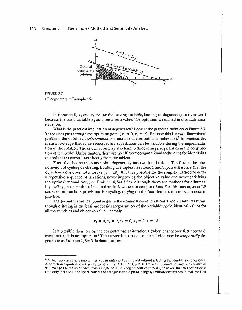
114 Chapter: 3 The Simplex Method and Sensitivity Analysis
- ----.... ~"""3........ ~I-7-9-_ :.t:
.... _2-....------fiGURE 3.7
LP degeneracy in Example 3.5-1
In iteration 0, X3 and X4 tie for the leaving variable, leading to degeneracy in iteration 1because the basic variable X4 assumes a zero value. The optimum is reached in one additionaliteration.
What is the practical implication of degeneracy? Look at the graphical solution in Figure 3.7.Three lines pass through the optimum point (Xl = 0, X2 = 2). Because this is a two-dimensionalproblem, the point is overdetermined and one of the constraints is redundant? In practice, themere knowledge that some resources are superfluous can be valuable during the implementation of the solution. The information may also lead to discovering irregularities in the construction of the model. Unfortunately, there are no efficient computational techniques for identifyingthe redundant constraints directly from the tableau.
From the theoretical standpoint, degeneracy has two implications. The first is the phenomenon of cycling or circling. Looking at simplex iterations 1 and 2, you will notice that theobjective value does not improve (z = 18). It is thus possible for the simplex method to entera repetitive sequence of iterations, never improving the objective value and never satisfyingthe optimality condition (see Problem 4, Set 3.5a). Although there are methods for eliminating cycling, these methods lead to drastic slowdown in computations. For this reason, most LPcodes do not include provisions for cycling, relying on the fact that it is a rare occurrence inpractice.
The second theoretical point arises in the examination of iterations 1 and 2. Both iterations,though differing in the basic-nonbasic categorization of the variables, yield identical values forall the variables and objective value-namely,
Is it possible then to stop the computations at iteration 1 (when degeneracy first appears),even though it is not optimum? The answer is no, because the solution may be temporarily degenerate as Problem 2, Set 3.5a demonstrates.
2Redundancy generally implies that constraints can be removed without affecting the feasible solution space.A sometimes quoted counterexample is x + y s 1, x ;:: 1, Y ;:: O. Here, the removal of anyone constraintwill change the feasible space from a single point to a region. Suffice it to say, however, that this condition istrue only if the solution space consists of a single feasible point, a highly unlikely occurrence in real-life LPs.
t,i[t
f~Ir
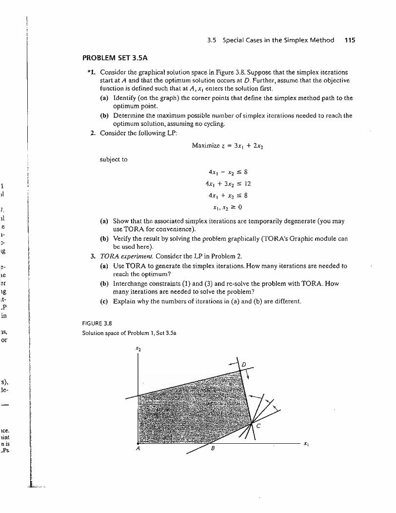
3.5 Special Cases in the Simplex Method 115
PROBLEM SET 3.5A
*1. Consider the graphical solution space in Figure 3.8. Suppose that the simplex iterationsstart at A and that the optimum solution occurs at D. Further, assume that the objectivefunction is defined such that at A, XI enters the solution first.
(a) Identify (on the graph) the corner points that define the simplex method path to theoptimum point.
(b) Determine the maximum possible number of simplex iterations needed to reach theoptimum solution, assuming no cycling.
2. Consider the following LP:
Maximize z = 3Xl + 2X2
subject to
1II
4xI - X2 ::; 8
4xI + 3X2 ::; 12
4xl + X2 ::; 8
"--------------- Xl
X2
(a) Show that the associated simplex iterations are temporarily degenerate (you mayuse TORA for convenience).
(b) Verify the result by solving the problem graphically (TORA's Graphic module canbe used here).
3. TORA experiment. Consider the LP in Problem 2.
(a) Use TORA to generate the simplex iterations. How many iterations are needed toreach the optimum?
(b) Interchange constraints (1) and (3) and re-solve the problem with TORA. Howmany iterations are needed to solve the problem?
(c) Explain why the numbers of iterations in (a) and (b) are different.
FIGURE 3.8
Solution space of Problem 1, Set 3.SalS,
or
s),le-
Ice.lintn is,Ps.
IgIt,Pin
7.11.e1-
116 Chapter 3 The Simplex Method and Sensitivity Analysis
4. TORA Experiment Consider the following LP (authored by E.M. Beale to demonstratecycling):
subject to
!x\ - 12x2 - !X3 + 3X4 :s; 0
X3 :s; 1
From TORA's SOLVEIMODIFY menu, select SolVe => Alge.l?,riiic. => Iterations =>All~slack. Next, "thumb" through the successive simplex iterations using the commandNext:ite'r-ati6h (do not use AltIterations, because the simplex method will then cycle indefinitely). You will notice that the starting all-slack basic feasible solution at iteration 0will reappear identically in iteration 6. This example illustrates the occurrence of cyclingin the simplex iterations and the possibility that the algorithm may never converge to theoptimum solution.
It is interesting that cycling will not occur in this example if all the coefficients in thisLP are converted to integer values by using proper multiples (try it!).
3.5.2 Alternative Optima
When the objective function is parallel to a nonredundant binding constraint (i.e., aconstraint that is satisfied as an equation at the optimal solution), the objectivefunction can assume the same optimal value at more than one solution point, thusgiving rise to alternative optima. The next example shows that there is an infinitenumber of such solutions. It also demonstrates the practical significance of encountering such solutions.
Example 3.5-2 (Infinite Number of Solutions)
Maximize z = 2Xl + 4X2
subject to
Xl + 2X2 :s; 5
Xl + X2:S; 4
Figure 3.9 demonstrates how alternative optima can arise in the LP model when the objective function is parallel to a binding constraint. Any point on the line segment Be represents analternative optimum with the same objective value z == 10.
The iterations of the model are given by the following tableaus.
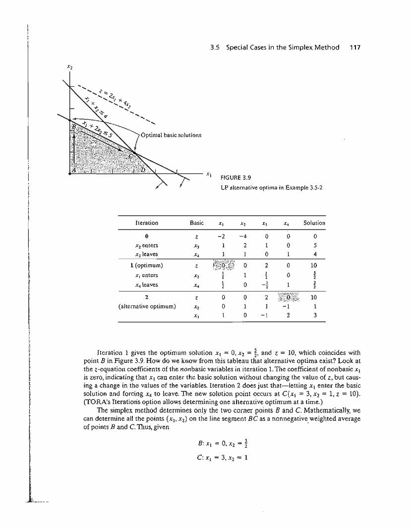
3.5 Special Cases in the Simplex Method 117
Optimal basic solutions
FIGURE 3.9
LP alternative optima in Example 3.5-2
Iteration Basic XI Xz X3 X4 Solution
0 Z -2 -4 0 0 0
Xz enters X3 1 2 1 0 5
x31eaves X4 1 ) 0 1 4
1 (optimum) Z ~i.~:{tgi~!i? 0 2 0 10
XI enters I 1 I 0 5Xz 2 2 2
x41eaves I 0 I 1 3X4 2 -2 2
2 z 0 0 2 ~f~)r~9:j~~~ 10
(alterna tive optimum) Xz 0 1 1 -1 1
XI 1 0 -) 2 3
Iteration 1 gives the optimum solution Xl = 0, x2 = t and z = 10, which coincides withpoint B in Figure 3.9. How do we know from this tableau that alternative optima exist? Look atthe z-equation coefficients of the nonbasic variables in iteration 1. The coefficient of nonbasic Xl
is zero, indicating that Xl can enter the basic solution without changing the value of z, but causing a change in the values of the variables. Iteration 2 does just that-letting Xl enter the basicsolution and forcing X4 to leave. The new solution point occurs at C(XI = 3, X2 = 1, z = 10).(TORA's Iteratioris option allows determining one alternative optimum at a time.)
The simplex method determines only the two corner points Band C. Mathematically, wecan determine all the points (Xl> X2) on the line segment Be as a nonnegative. weighted averageof points Band C. TIlUS, given
118 Chapter 3 The Simplex Method and Sensitivity Analysis
then all the points on the line segment BC are given by
Xl = 0'(0) + (1 - a)(3) = 3 - 3a} °A (5) 3 , :5 a :5 1x2 = a 2 + (1 - a)(l) = 1 + 2a
When a = 0, (x), X2) = (3,1), which is point C. When a = 1, (Xl> X2) = (0, n, which ispoint B. For values of a between °and 1, (xt> ot-2) lies between Band C.
Remarks. In practice, alternative optima are useful because we can choose from many solutions without experiencing deterioration in the objective value. For instance, in the present example, the solution at B shows that activity 2 only is at a positive level, whereas at C bothactivities are positive. If the example represents a product-mix situation, there may be advantages in producing two products rather than one to meet market competition. In this ease, the solution at C may be more appealing.
PROBLEM SeT 3.5B
*1. For the following LP, identify three alternative optimal basic solutions, and then write ageneral expression for all the nonbasic alternative optima comprising these three basicsolutions.
Maximize z =: Xl + 2X2 + 3X3
subject to
Xl + 2x2 + 3X3 :%: 10
XI + x2 :%: 5
Xl :%: 1
Note: Although the problem has more than three alternative basic solution optima,you are only required to identify three of them. You may use TORA forconvenience.
2. Solve the following LP:
Maximize z = 2Xl - X2 + 3X3
subject to
Xl - X2 + 5X3 :%: 10
2Xl - X2 + 3x3 :%: 40
From the optimal tableau, show that all the alternative optima are not corner points(i.e., nonbasic). Give a two-dimensional graphical demonstration of the type of solution space and objective function that will produce this result. (You may use TORAfor convenience.)
f{,f
f[:IrI!
3
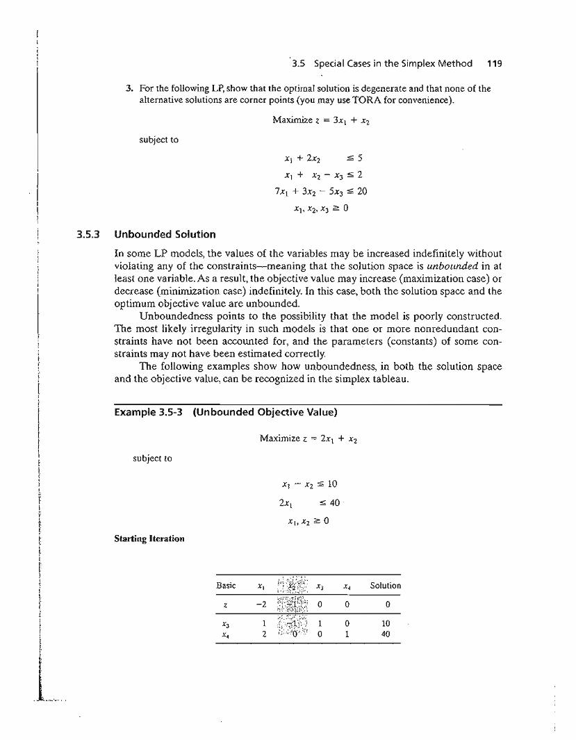
3.5 . Special Cases in the Simplex Method 119
3. For the following LP, show that the optimal solution is degenerate and that none of thealternative solutions are corner points (you may use TORA for convenience).
Maximize z = 3XI + Xl
subject to
Xl + 2X2 :5 5
Xl + X2 - x3 :5 2
7XI + 3X2 - 5X3 :5 20
3.5.3 Unbounded Solution
In some LP models, the values of the variables may be increased indefinitely withoutviolating any of the constraints-meaning that the solution space is unbounded in atleast one variable. As a result, the objective value may increase (maximization case) ordecrease (minimization case) indefinitely. In this case, both the solution space and theoptimum objective value are unbounded.
Unboundedness points to the possibility that the model is poorly constructed.The most likely irregularity in such models is that one or more nonredundant constraints have not been accounted for, and the parameters (constants) of some constraints may not have been estimated correctly.
The following examples show how unboundedness, in both the solution spaceand the objective value, can be recognized in the simplex tableau.
Example 3.5-3 (Unbounded Objective Value)
Maximize z = 2xl + X2
subject to
Starting Iteration
Basic Xl n;~~:~:r X3 X4 Solution
z -2 !f.if;~r{ml~~ 0 0 0
X3 1 iJ~;:~~if.r~ 1 0 10X4 2 0 1 40
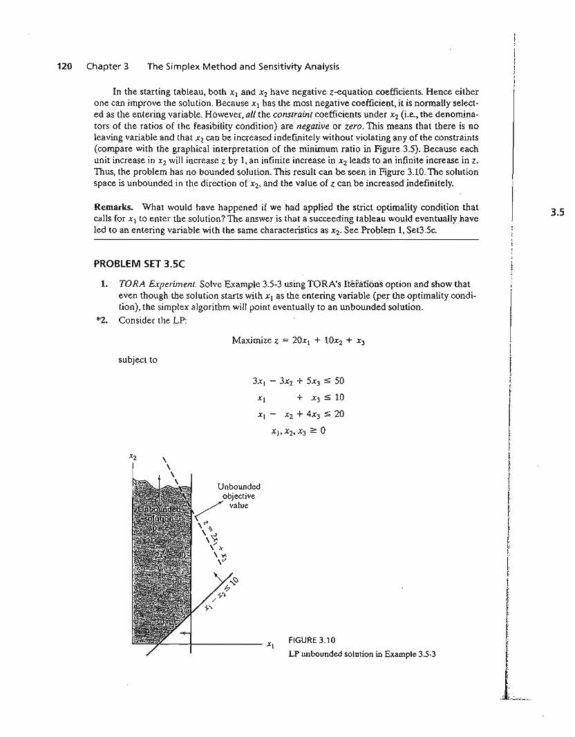
120 Chapter 3 The Simplex Method and Sensitivity Analysis
In the starting tableau, both Xl and X2 have negative z-equation coefficients. Hence eitherone can improve the solution. Because Xl has the most negative coefficient, it is normally selected as the entering variable. However, all the constraint coefficients under X2 (Le., the denominators of the ratios of the feasibility condition) are negative or zero. This means that there is noleaving variable and that X2 can be increased indefinitely without violating any of the constraints(compare with the graphical interpretation of the minimum ratio in Figure 3.5). Because eachunit increase in Xl will increase z by 1, an infinite increase in X2 leads to an infinite increase in z.Thus, the problem has no bounded solution. This result can be seen in Figure 3.10. The solutionspace is unbounded in the direction of X2, and the value of z can be increased indefinitely.
Remarks. What would have happened if we had applied the strict optimality condition thatcalls for Xl to enter the solution? The answer is that a succeeding tableau would eventually haveled to an entering variable with the same characteristics as X2' See Problem 1, Set3.5c.
PROBLEM SET 3.Se
1. TORA Experiment. Solve Example 3.5-3 using TORA's Iterations option and show thateven though the solution starts with Xl as the entering variable (per the optimality condition), the simplex algorithm will point eventually to an unbounded solution.
*2. Consider the LP:
Maximize z = 20XI + lOx2 + X3
subject to
3Xl - 3X2 + 5X3 :$; 50
Xl + x3::; 10
Xl - X2 + 4x3 ::; 20
3.5
Unboundedobjective~ value
\T\\~\"
\ >r,~
,">
~--f------- XlFIGURE 3.10
LP unbounded solution in Example 3.5-3
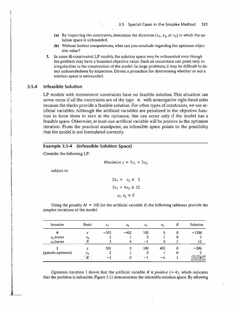
3.5 Special Cases in the Simplex Method 121
(a) By inspecting the constraints, determine the direction (XI. X2, or X3) in which the solution space is unbounded.
(b) Without further computations, what can you conclude regarding the optimum objective value?
3. In some ill-constructed LP models, the solution space may be unbounded even thoughthe problem may have a bounded objective value. Such an occurrence can point only toirregularities in the construction of the model. In large problems, it may be difficult to detect unboundedness by inspection. Devise a procedure for determining whether or not asolution space is unbounded.
3.5.4 Infeasible Solution
LP models with inconsistent constraints have no feasible solution. This situation cannever occur if all the constraints are of the type <: with nonnegative right-hand sidesbecause the slacks provide a feasible solution. For other types of constraints, we use artificial variables. Although the artificial variables are penalized in the objective function to force them to zero at the optimum, this can occur only if the model has afeasible space. Otherwise, at least one artificial variable will be positive in the optimumiteration. From the practical standpoint, an infeasible space points to the possibilitythat the model is not formulated correctly.
Example 3.5-4 (Infeasible Solution Space)
Consider the following LP:
Maximize z = 3x) + 2X2
subject to
Using the penalty M = 100 for the artificial variable R, the following tableaux provide thesimplex iterations of the model.
Iteration Basic Xl X2 X4 X3 R Solution
0 z -303 -402 100 0 0 -1200Xz enters X3 2 1 0 1 0 2x3leaves R 3 4 -1 0 1 12
1 z 501 0 100 402 0 -396(pseudo-optimum) X2 2 1 0 1 0 2
: R" -5 0 -1 -4 1 ~~~~l{~~~fI;~
Optimum iteration 1 shows that the artificial variable R is positive (= 4), which indicatesthat the problem is infeasible. Figure 3.11 demonstrates the infeasible solution space. By allowing
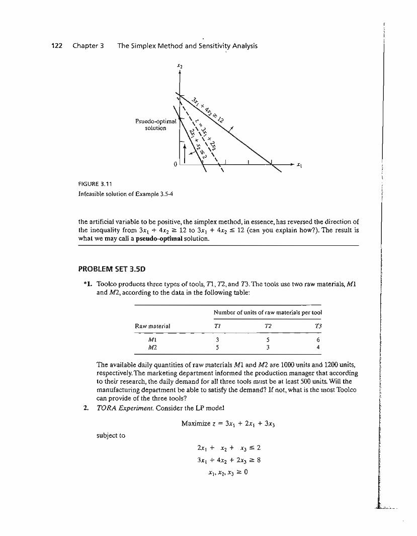
122 Chapter 3 The Simplex Method and Sensitivity Analysis
Psuedo-optimalsolution
oL.....:...----'r-'\-.......--.......---"'~--- ;1:1
FIGURE 3.11
Infeasible solution of Example 3.5-4
the artificial variable to be positive, the simplex method, in essence, has reversed the direction ofthe inequality from 3X1 + 4X2 ;;;0: 12 to 3Xl + 4X2 ~ 12 (can you explain how?). The result iswhat we may call a pseudo-optimal solution.
PROBLEM SET 3.50
*1. Tooleo produces three types of tools, 71, n, and 13. The tools use two raw materials, M1and M2, according to the data in the following table:
Number of units of raw materials per tool
Maximize z = 3XI + 2Xl + 3X3
subject to
64
T3
53
72
35
Tl
2Xl + X2 + X3 ~ 2
3xI + 4x2 + 2X3 ;;;0: 8
MlM2
Raw material
The available daily quantities of raw materials M1 and M2 are 1000 units and 1200 units,respectively. The marketing department informed the production manager that accordingto their research, the daily demand for all three tools must be at least 500 units. Will themanufacturing department be able to satisfy the demand? If not, what is the most Toolcocan provide of the three tools?
TORA Experiment. Consider the LP model2.
3.6 Sensitivity Analysis 123
Use TORA's Iterations => M~Meth6d to show that the optimal solution includes an artificial basic variable, but at zero level. Does the problem have a feasible optimal solution?
3.6 SENSITIVITY ANALYSIS
ofIS
In LP, the parameters (input data) of the model can change within certain limits without causing the optimum solution to change. This is referred to as sensitivity analysis,and will be the subject matter of this section. Later, in Chapter 4, we will study postoptimal analysis which deals with determining the new optimum solution resultingfrom making targeted changes in the input data.
In LP models, the parameters are usually not exact. With sensitivity analysis, wecan ascertain the impact of this uncertainty on the quality of the optimum solution. Forexample, for an estimated unit profit of a product, if sensitivity analysis reveals that theoptimum remains the same for a ±1O% change in the unit profit, we can conclude thatthe solution is more robust than in the case where the indifference range is only ±1 %.
We will start with the more concrete graphical solution to explain the basics ofsensitivity analysis. These basics will then be extended to the general LP problem usingthe simplex tableau results.
3.6.1 Graphical Sensitivity Analysis
This section demonstrates the general idea of sensitivity analysis. Two cases will be considered:
'1 1. Sensitivity of the optimum solution to changes in the availability of the resources(right-hand side of the constraints).
2. Sensitivity of the optimum solution to changes in unit profit or unit cost (coefficients of the objective function).
Example 3.6-1 (Changes in the Right-Hand Side)
Maximize z = 30Xl + 20X2
(Machine 1)
(Machine 2)
2Xl + X2 s; 8
Xl + 3X2 :5 8
We will consider the two cases separately, using examples of two-variable graphical LPs.
subject to
JOBCO produces two products on two machines. A unit of product 1 requires 2 hours on machine1 and 1 hour on machine 2. For product 2, a unit requires 1 hour on machine 1 and 3 hours on machine 2. The revenues per unit of products 1 and 2 are $30 and $20, respectively. The total dailyprocessing time available for each machine is 8 hours.
Letting Xl and X2 represent the daily number of units of products 1 and 2, respectively, theLP model is given as
ng
co
:s,
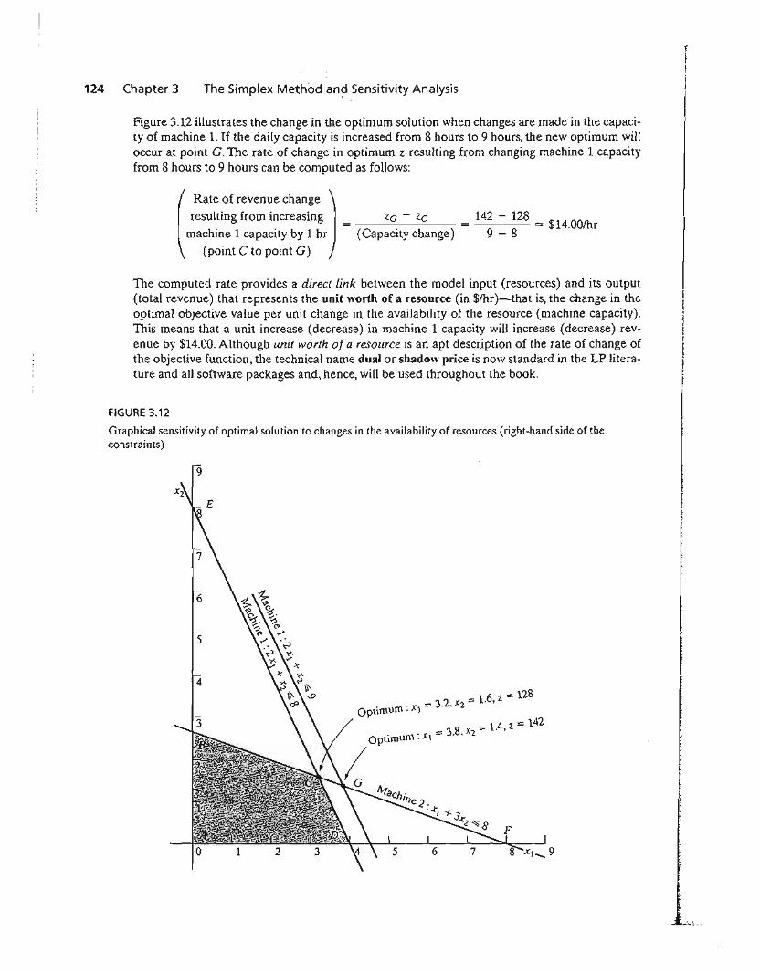
124 Chapter 3 The Simplex Method an~ Sensitivity Analysis
Figure 3.12 illustrates the change in the optimum solution when changes are made in the capacity of machine 1. If the daily capacity is increased from 8 hours to 9 hours, the new optimum willoccur at point G. The rate of change in optimum z resulting from changing machine 1 capacityfrom 8 hours to 9 hours can be computed as follows:
(
Rate of revenue change )resulting from increasing Ze - Zc
machine 1 capacity by 1 hr - (Capacity change)(point C to point G)
142 - 128 = $14.00/hr9 - 8
The computed rate provides a direct link between the model input (resources) and its output(total revenue) that represents the unit worth of a resource (in $/hr)-that is, the change in theoptimal objective value per unit change in the availability of the resource (machine capacity).This means that a unit increase (decrease) in machine 1 capacity will increase (decrease) revenue by $14.00. Although unit worth of a resource is an apt description of the rate of change ofthe objective function, the technical name dual or shadow price is now standard in the LP literature and all software packages and, hence, will be used throughout the book.
FIGURE 3.12
Graphical sensitivity of optimal solurion to changes in the availability of resources (right-hand side of theconstraints)
9
6
5
4
16 == 128. • == 3:2,.x:2 == . ,z
Optlmurn . Xl
X == 1.4. Z == 142. rn . Xl == 3.8, 2 ';;OPhmu.
"'taCh'll]e2 .
• 4-/ 1- 3-r~~8
-'...:.,--
3.6 Sensitivity Analysis 125
Looking at Figure 3.12, we can see that the dual price of $14.00/hr remains valid for changes(increases or decreases) in machine 1 capacity that move its constraint parallel to itself to anypoint on the line segment BF. This means that the range of applicability of the given dual pricecan be computed as follows:
Minimum machine 1 capacity [at B = (0,2.67)] = 2 x 0 + 1 x 2.67 = 2.67 hr
Maximum machine 1 capacity [at F '"' (8,0)] = 2 x 8 + 1 x 0 = 16 hr
We can thus conclude that the dual price of $14.00/hr will remain valid for the range
2.67 hrs :5 Machine 1 capacity :5 16 hrs
Changes outside this range will produce a different dual price (worth per unit).Using similar computations, you can verify that the dual price for machine 2 capacity is
$2.00/hr and it remains valid for changes (increases or decreases) that move its constraint parallel to itself to any point on the line segment DE, which yields the following limits:
Minimum machine 2 capacity [at D = (4,0)] = 1 x 4 + 3 X a = 4 hr
Maximum machine 2 capacity [at E = (8, 0)] = 1 x a + 3 x 8 = 24 hr
The conclusion is that the dual price of $2.00/hr for machine 2 will remain applicable for the range
4 hr :5 Machine 2 capacity :5 24 hr
The computed limits for machine 1 and 2 are referred to as the feasibility ranges. All softwarepackages provide information about the dual prices and their feasibility ranges. Section 3.6.4shows how AMPL, Solver, and TORA generate this information.
The dual prices allow making economic decisions about the LP problem, as the followingquestions demonstrate:
Question 1. If JOBCO can increase the capacity of both machines, which machine should receive higher priority?
The dual prices for machines 1 and 2 are $14.00/hr and $2.00/hr. TIlis means that each additional hour of machine 1 will increase revenue by $14.00, as opposed to only $2.00 for machine 2.Thus, priority should be given to machine 1.
Question 2. A suggestion is made to increase the capacities of machines 1 and 2 at the additional cost of $10/hr. Is this advisable?
For machine 1, the additional net revenue per hour is 14.00 - 10.00 = $4.00 and for machine 2, the net is $2.00 - $10.00 = -$8.00. Hence, only the capacity of machine 1 should beincreased.
Question 3. If the capacity of machine 1 is increased from the present 8 hours to 13 hours, howwill this increase impact the optimum revenue?
The dual price for machine 1 is $14.00 and is applicable in the range (2.67,16) hr. TIle proposed increase to 13 hours falls within the feasibility range. Hence, the increase in revenue is$14.00(13 - 8) = $70.00, which means that the total revenue will be increased to(current revenue + change in revenue) = 128 + 70 = $198.00.
Question 4. Suppose that the capacity of machine 1 is increased to 20 hours, how will this increase impact the optimum revenue?
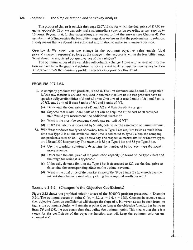
126 Chapter 3 The Simplex Method and Sensitivity Analysis
The proposed change is outside the range (2.67, 16) hr for which the dual price of $14.00 remains applicable. Thus, we can only make an immediate conclusion regarding an increase up to16 hours. Beyond that, further calculations are needed to find the answer (see Chapter 4). Remember that falling outside the feasibility range does not mean that the problem has no solution.It only means that we do not have sufficient information to make an immediate decision.
Question 5. We know that the change in the optimum objective value equals (dualprice X change in resource) so long as the change in the resource is within the feasibility range.What about the associated optimum values of the variables?
The optimum values of the variables will definitely change. However, the level of information we have from the graphical solution is not sufficient to determine the new values. Section3.6.2, which treats the sensitivity problem algebraically, provides this detail.
PROBLEM SET 3.6A
1. A company produces two products, A and B. The unit revenues are $2 and $3, respectively. Two raw materials, M1 and M2, used in the manufacture of the two products have respective daily availabilities of 8 and 18 units. One unit of A uses 2 units of Ml and 2 unitsof M2, and 1 unit of Buses 3 units of Ml and 6 units of M2.
(a) Determine the dual prices of Ml and M2 and their feasibility ranges.
(b) Suppose that 4 additional units of Ml can be acquired at the cost of 30 cents perunit. Would you recommend the additional purchase?
(c) What is the most the company should pay per unit of M2?
(d) If M2 availability is increased by 5 units, determine the associated optimum revenue.
*2. Wild West produces two types of cowboy hats. A Type 1 hat requires twice as much labortime as a Type 2. If all the available labor time is dedicated to Type 2 alone, the companycan produce a total of 400 Type 2 hats a day. The respective market limits for the two typesare 150 and 200 hats per day. The revenue is $8 per Type 1 hat and $5 per Type 2 hat.
(a) Use the graphical solution to determine the number of hats of each type that maximizes revenue.
(b) Determine the dual price of the production capacity (in terms of the Type 2 hat) andthe range for which it is applicable.
(c) If the daily demand limit on the Type 1 hat is decreased to 120, use the dual price todetermine the corresponding effect on the optimal revenue.
(d) What is the dual price of the market share of the Type 2 hat? By how much can themarket share be increased while yielding the computed worth per unit?
Example 3.6-2 (Changes in the Objective Coefficients)
Figure 3.13 shows the graphical solution space of the lOBeO problem presented in Example3.6-1. The optimum occurs at point C (Xl == 3.2, Xl = 1.6, Z == 128). Changes in revenue units(i.e., objective-function coefficients) will change the slope of z. However, as can be seen from thefigure, the optimum solution will remain at point C so long as the objective function lies betweenlines BF and DE, the two constraints that define the optimum point. This means that there is arange for the coefficients of the objective function that will keep the optimum solution unchanged at C.
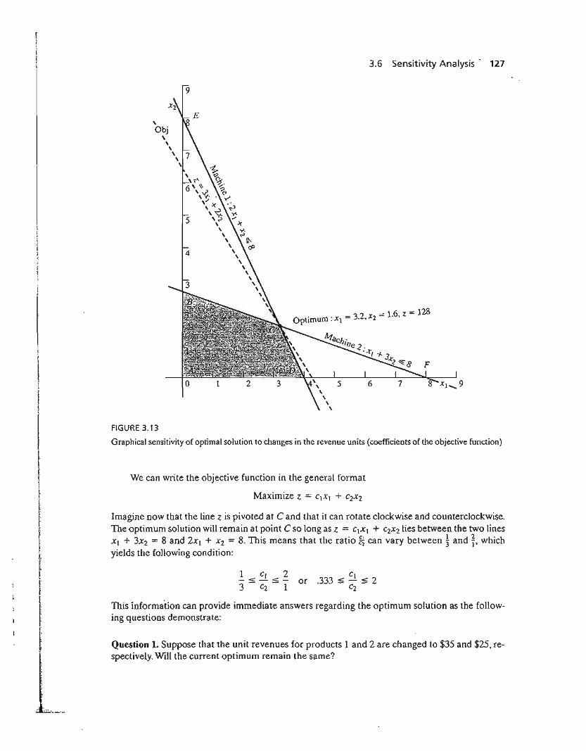
3.6 Sensitivity Analysis' 127
9
'\
Obj'\
'\'\'\
'\'\
5
4
3 2 - 16 z = 128Optimum :x\ = . ,x2 - . ,
Nrach'1l1e 2.
·.r, -f-.3~2~8
FIGURE 3.13
Graphical sensitivity of optimal solution to changes in the revenue units (coefficients of the objective function)
We can write the objective function in the general format
Maximize z = C\Xl + c2x2
Imagine now that the line z is pivoted at C and that it can rotate clockwise and counterclockwise.The optimum solution will remain at point C so long as Z = C\X\ + c2x2lies between the two linesXl + 3X2 = 8 and 2Xl + X2 = 8. This means that the ratio ~ can vary between ~ and t, whichyields the following condition:
1 CI 2-<-<-3 - C2 - 1
or .333:$ Cl :$ 2C2
This information can provide immediate answers regarding the optimum solution as the following questions demonstrate:
Question 1. Suppose that the unit revenues for products 1 and 2 are changed to $35 and $25, respectively. Will the current optimum remain the same?
128 Chapter 3 The Simplex Method and Sensitivity Analysis
The new objective function is
Maximize z = 35xI + 25x2
The solution at C will remain optimal because ~ == ~ = 1.4 remains within the optimality range(.333,2). When the ratio falls outside this range, additional calculations are needed to find the newoptimum (see Chapter 4). Notice that although the values of the variables at the optimum point Cremain unchanged, the optimum value of z changes to 35 X (3.2) + 25 X (1.6) == $152.00.
Question 2. Suppose that the unit revenue of product 2 is fixed at its current value ofc2 = $20.00. What is the associated range for Cj, the unit revenue for product 1 that will keep theoptimum unchanged?
Substituting C2 = 20 in the condition ~ ~ ~ ~ 2, we get
! X 20 ::; Cl ~ 2 x 20
Or
6.67 ~ Cl ~ 40
This range is referred to as the optimality range for Cb and it implicitly assumes that C2 is fixed at$20.00.
We can similarly determine the optimality range for C2 by fixing the value of Ct at $30.00. Thus,
Or
As in the case of the right-hand side, all software packages provide the optimality ranges.Section 3.6.4 shows how AMPL, Solver, and TORA generate these results.
Remark. Although the material in this section has dealt only with two variables, the resultslay the foundation for the development of sensitivity analysis for the general LP problem inSections 3.6.2 and 3.6.3.
PROBLEM SET 3.6B
1. Consider Problem 1, Set 3.6a.
(a) Determine the optimality condition for ~ that will keep the optimum unchanged.
(b) Determine the optimality ranges for CA and C8, assuming that the other coefficient iskept constant at its present value.
(c) If the unit revenues CA and CB are changed simultaneously to $5 and $4, respectively,determine the new optimum solution.
(d) If the changes in (c) are made one at a time, what can be said about the optimumsolution?
2. In the Reddy Mikks model of Example 2.2-1;
(a) Determine the range for the ratio of the unit revenue of exterior paint to the unitrevenue of interior paint.
t
I~
3
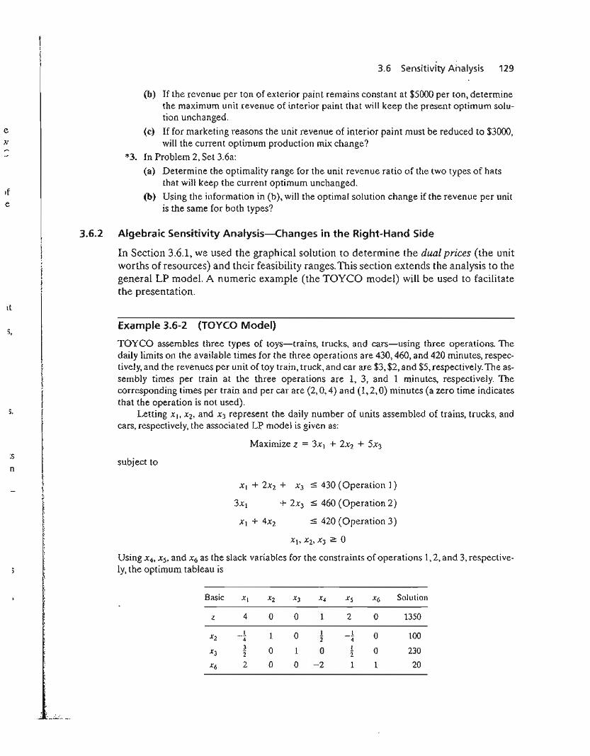
e.v
Ife
5,
s.
:s
n
3.6 Sensitivity Analysis 129
(b) If the revenue per ton of exterior paint remains constant at $5000 per ton, determinethe maximum unit revenue of interior paint that will keep the present optimum solution unchanged.
(c) If for marketing reasons the unit revenue of interior paint must be reduced to $3000,will the current optimum production mix change?
*3. In Problem 2, Set 3.6a:
(a) Determine the optimality range for the unit revenue ratio of the two types of hatsthat will keep the current optimum unchanged.
(b) Using the information in (b), will the optimal solution change if the revenue per unitis the same for both types?
3.6.2 Algebraic Sensitivity Analysis-Changes in the Right-Hand Side
In Section 3.6.1, we used the graphical solution to determine the dual prices (the unitworths of resources) and their feasibility ranges. This section extends the analysis to thegeneral LP model. A numeric example (the TOYCO model) will be used to facilitatethe presentation.
Example 3.6-2 (TOYCO Model)
TOYCO assembles three types of toys-trains, trucks, and cars-using three operations. Thedaily limits on the available times for the three operations are 430,460, and 420 minutes, respectively, and the revenues per unit of toy train, truck, and car are $3, $2, and $5, respectively. The assembly times per train at the three operations are 1, 3, and 1 minutes, respectively. Thecorresponding times per train and per car are (2,0,4) and (1,2,0) minutes (a zero time indicatesthat the operation is not used).
Letting Xl> X2, and X3 represent the daily number of units assembled of trains, trucks, andcars, respectively, the associated LP model is given as:
Maximize z = 3x, + 2X2 + 5X3
subject to
:s 430 (Operation] )
:s 460 (Operation 2)
:s 420 (Operation 3)
- '-~
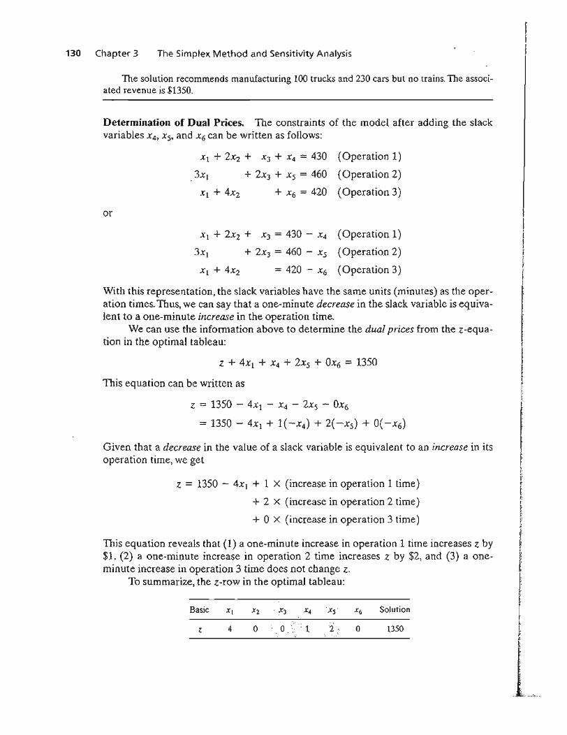
130 Chapter 3 The Simplex Method and Sensitivity Analysis
The solution recommends manufacturing 100 trucks and 230 cars but no trains. The associated revenue is $1350.
Determination of Dual Prices. The constraints of the model after adding the slackvariables X4, Xs, and x6 can be written as follows:
Xl + 2X2 + X3 + X4 = 430 (Operation 1)
.3XI + 2X3 + Xs = 460 (Operation 2)
xl + 4X2 + X6 = 420 (Operation 3)
or
Xl + 2X2 + X3 = 430 - X4
3XI + 2X3 = 460 - Xs
Xl + 4X2 = 420 - x6
(Operation 1)
(Operation 2)
(Operation 3)
With this representation, the slack variables have the same units (minutes) as the operation times. Thus, we can say that a one-minute decrease in the slack variable is equivalent to a one-minute increase in the operation time.
We can use the information above to determine the dual prices from the z-equation in the optimal tableau:
z + 4XI + X4 + 2xs + OX6 = 1350
This equation can be written as
z = 1350 - 4XI - X4 - 2xs - OX6
= 1350 - 4Xl + 1(-x4) + 2(-xs) + 0(-X6)
Given that a decrease in the value of a slack variable is equivalent to an increase in itsoperation time, we get
z = 1350 - 4XI + 1 X (increase in operation 1 time)
+ 2 X (increase in operation 2 time)
+ 0 x (increase in operation 3 time)
This equation reveals that (1) a one-minute increase in operation 1 time increases z by$1, (2) a one-minute increase in operation 2 time increases z by $2, and (3) a oneminute increase in operation 3 time does not change z.
To summarize, the z-row in the optimal tableau:
Basic
4
X2 ..X3 X4 -Xs X6
0 0 1 2 0
Solution
1350
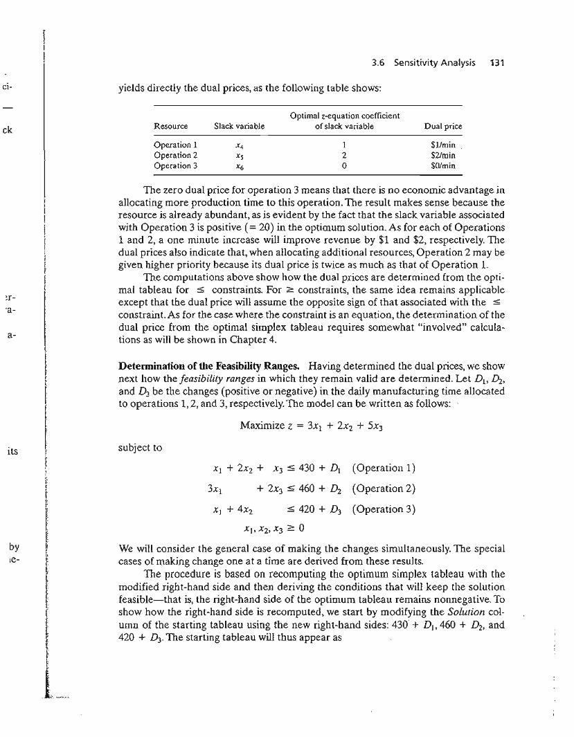
Cl-
3.6 Sensitivity Analysis 131
yields directly the dual prices, as the following table shows:
Optimal z-equation coefficient
ck Resource Slack variable of slack variable Dual price
Operation 1 X4 1 $lIminOperation 2 Xs 2 $2/minOperation 3 X6 0 SO/min
~r-
.a-
its
The zero dual price for operation 3 means that there is no economic advantage inallocating more production time to this operation. The result makes sense because theresource is already abundant, as is evident by the fact that the slack variable associatedwith Operation 3 is positive (= 20) in the optimum solution. As for each of Operations1 and 2, a one minute increase will improve revenue by $1 and $2, respectively. Thedual prices also indicate that, when allocating additional resources, Operation 2 may begiven higher priority because its dual price is twice as much as that of Operation 1.
The computations above show how the dual prices are determined from the optimal tableau for ~ constraints. For > constraints, the same idea remains applicableexcept that the dual price will assume the opposite sign of that associated with the :5
constraint. As for the case where the constraint is an equation, the determination of thedual price from the optimal simplex tableau requires somewhat "involved" calculations as will be shown in Chapter 4.
Determination of the Feasibility Ranges. Having determined the dual prices, we shownext how the feasibility ranges in which they remain valid are determined. Let D I , Dz,and D3 be the changes (positive or negative) in the daily manufacturing time allocatedto operations 1,2, and 3, respectively. The model can be written as follows:
Maximize z = 3Xl + 2x2 + 5X3
subject to
X I + 2xz + x3:5 430 + DI (Operation 1)
3xi + 2X3 :::; 460 + Dz (Operation 2)
Xl + 4X2 :5 420 + D3 (Operation 3)
We will consider the general case of making the changes simultaneously. The specialcases of making change one at a time are derived from these results.
The procedure is based on recomputing the optimum simplex tableau with themodified right-hand side and then deriving the conditions that will keep the solutionfeasible-that is, the right-hand side of the optimum tableau remains nonnegative. Toshow how the right-hand side is recomputed, we start by modifying the Solution column of the starting tableau using the new right-hand sides: 430 + Db 460 + Dz, and420 + D3. The starting tableau will thus appear as
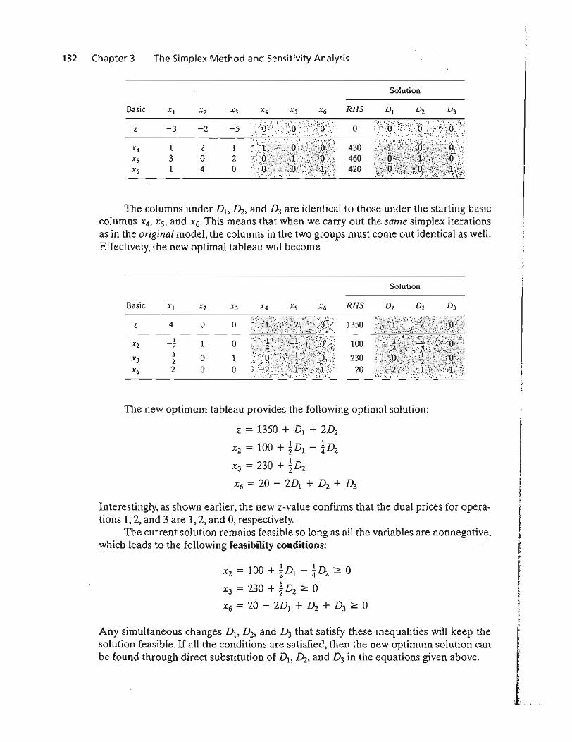
132 Chapter 3 The Simplex Method and Sensitivity Analysis
Solution
Basic Xl' X2 X3
Z -3 -2 -5
X4 1 2 1Xs 3 0 2X6 1 4 0
The columns under Db Dz, and D3 are identical to those under the starting basiccolumns X4, xs, and X6' This means that when we carry out the same simplex iterationsas in the original model, the columns in the two groups must come out identical as well.Effectively, the new optimal tableau will become
Solution
Basic Xl X2
Z 4 0
I 1X2 -43 0X3 2
X6 2 0
o
o1
o
The new optimum tableau provides the following optimal solution:
z = 1350 + D1 + 2Dz1 1
Xz = 100 + '2 D} - 4 Dz
x3 = 230 + ~D2
x6 = 20 - 2D1 + Dz + D3
Interestingly, as shown earlier, the new z-value confirms that the dual prices for operations 1,2, and 3 are 1,2, and 0, respectively.
The current solution remains feasible so long as all the variables are nonnegative,which leads to the following feasibility conditions:
Xz = 100 + !D1 - ~ Dz ~ 0
x3 = 230 + ~ Dz ~ 0
X6 = 20 - 2D} + Dz + D3 ~ 0
Any simultaneous changes Db Dz, and DJ that satisfy these inequalities will keep thesolution feasible. If all the conditions are satisfied, then the new optimum solution canbe found through direct substitution of Db ~, and D3 in the equations given above.
3.6 Sensitivity Analysis 133
To illustrate the use of these conditions, suppose that the manufacturing timeavailable for operations 1,2, and 3 are 480,440, and 410 minutes respectively. Then, Dl =
480 - 430 = 50, ~ = 440 - 460 = -20, and D] = 410 - 420 = -10. Substitutingin the feasibility conditions, we get
X2 = 100 + ~(50) - ~(-20) = 130 > 0
x3 = 230 + ~(-20) = 220 > 0
X6 = 20 - 2(50) + (-20) + (-10) = -110 < 0
(feasible)
(feasible)
(infeasible)
cs
TIle calculations show that x6 < 0, hence the current solution does not remain feasible.Additional calculations will be needed to find the new solution. These calculations arediscussed in Chapter 4 as part of the post-optimal analysis.
Alternatively, if the changes in the resources are such that D1 = -30, Dz = -12,and D3 = 10, then
X2 = 100 + ~(-30) - h-12) = 88 > 0
X3 = 230 + ~(-12) = 224 > 0
x6 = 20 - 2(-30) + (-12) + (10) = 78 > 0
(feasible)
(feasible)
(feasible)
l;-I[I
~F
[
i" r
!~
~
~
rrt
"1
, .....:- .. --_ ..
The new feasible solution is Xl = 88, X3 = 224, and X6 = 68 with z = 3(0) + 2(88) +5(224) = $1296. Notice that the optimum objective value can also be computed asz = 1350 + 1( -30) + 2( -12) = $1296.
The given conditions can be specialized to produce the individual feasibility rangesthat result from changing the resources one at a time (as defined in Section 3.6.1).
Case 1. Change in operation 1 time from 460 to 460 + D} minutes. This change is equivalent to setting Dz = D3 = 0 in the simultaneous conditions, which yields
Xz = 100 + ~ D l ~ 0~ D[ ~ -200}X3 = 230 > 0 ~ -200 <: D1 :5 10x6 = 20 - 2D[ ~ 0 =} Dr :5 10
Case 2. Change in operation 2 time from 430 to 430 + Dzminutes. This change is equivalent to setting D1 = D3 = 0 in the simultaneous conditions, which yields
Case 3. Change in operation 3 time from 420 to 420 + D] minutes. This change is equivalent to setting D1 = Dz = 0 in the simultaneous conditions, which yields
X2 = 100> 0 }x3 = 230 > 0 ~ -20 :5 D3 < 00
X6 = 20 + D3 ~ 0
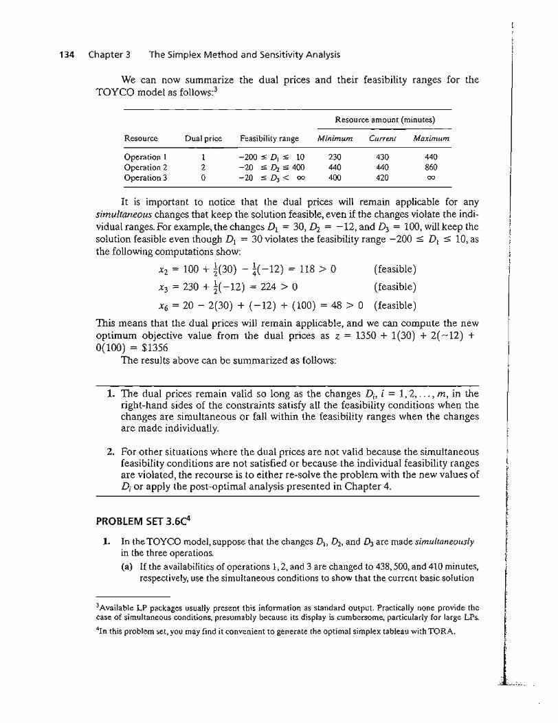
134 Chapter 3 The Simplex Method and Sensitivity Analysis
(feasible)
(feasible)
(feasible)
We can now summarize the dual prices and their feasibility ranges for theTOYCO model as follows:3
Resource amount (minutes)
Resource Dual price Feasibility range Minimum Current Maximum
Operation 1 1 -200::=;; D1 ::=;; 10 230 430 440Operation 2 2 -20 ::=;;D2 :$400 440 440 860Operation 3 0 -20 :$ D3 < 00 400 420 00
It is important to notice that the dual prices will remain applicable for anysimultaneous changes that keep the solution feasible, even if the changes violate the individual ranges. For example, the changes D1 = 30, Dz = -12, and D3 = 100, will keep thesolution feasible even though D] = 30 violates the feasibility range -200 ::s D l ::s 10, asthe following computations show:
Xz = 100 + ~(30) - ~(-12) = 118> 0
X3 = 230 + ~(-12) = 224 > 0
X6 = 20 - 2(30) + (-12) + (100) = 48 > 0
This means that the dual prices will remain applicable, and we can compute the newoptimum objective value from the dual prices as z = 1350 + 1(30) + 2( -12) +0(100) = $1356
The results above can be summarized as follows:
1. The dual prices remain valid so long as the changes Di , i = 1,2, ... , m, in theright-hand sides of the constraints satisfy all the feasibility conditions when thechanges are simultaneous or fall within the feasibility ranges when the changesare made individually.
2. For other situations where the dual prices are not valid because the simultaneousfeasibility conditions are not satisfied or because the individual feasibility rangesare violated, the recourse is to either re-solve the problem with the new values ofDi or apply the post-optimal analysis presented in Chapter 4.
PROBLEM SET 3.6et
1. In the TOYCO model, suppose that the changes DI , Dz, and D3 are made simultaneouslyin the three operations.(a) If the availabilities of operations 1,2, and 3 are changed to 438,500, and 410 minutes,
respectively, use the simultaneous conditions to show that the current basic solution
3Available LP packages usually present this information as standard output. Practically none provide thecase of simultaneous conditions, presumably because its display is cumbersome, particularly for large LPs.
41n this problem set, you may find it convenient to generate the optimal simplex tableau with TORA.
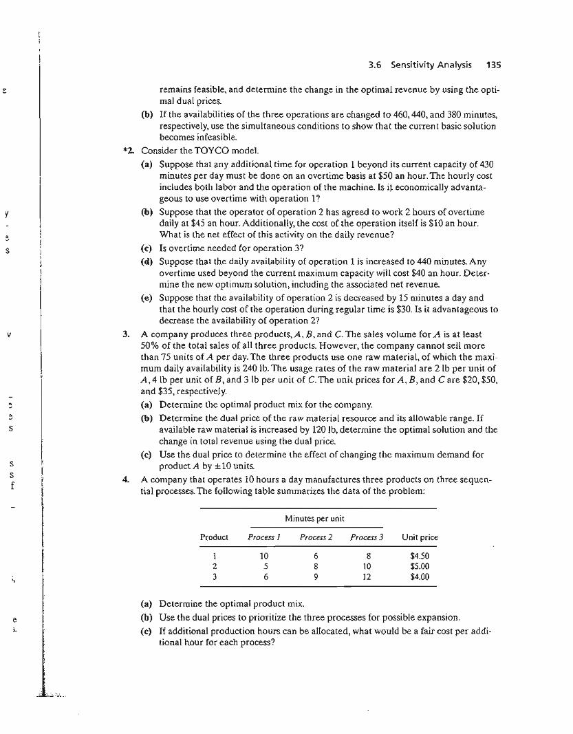
s
e
y
s
ssf
"
e,.
._.~ ....i;..: .....:.._.
3.6 Sensitivity Analysis 135
remains feasible, and determine the change in the optimal revenue by using the optimal dual prices.
(b) If the availabilities of the three operations are changed to 460,440, and 380 minutes,respectively, use the simultaneous conditions to show that the current basic solutionbecomes infeasible.
*2. Consider the TOYCO model.
(a) Suppose that any additional time for operation 1 beyond its current capacity of 430minutes per day must be done on an overtime basis at $50 an hour. The hourly costincludes both labor and the operation of the machine. Is it economically advantageous to use overtime with operation I?
(b) Suppose that the operator of operation 2 has agreed to work 2 hours of overtimedaily at $45 an hour. Additionally, the cost of the operation itself is $10 an hour.What is the net effect of this activity on the daily revenue?
(c) Is overtime needed for operation 3?
(d) Suppose that the daily availability of operation 1 is increased to 440 minutes. Anyovertime used beyond the current maximum capacity will cost $40 an hour. Determine the new optimum solution, including the associated net revenue.
(e) Suppose that the availability of operation 2 is decreased by 15 minutes a day andthat the hourly cost of the operation during regular time is $30. Is it advantageous todecrease the availability of operation 2?
3. A company produces three products, A, B, and C. The sales volume for A is at least50% of the total sales of all three products. However, the company cannot sell morethan 75 units of A per day. The three products use one raw material, of which the maximum daily availability is 240 lb. The usage rates of the raw material are 2 lb per unit ofA,4 lb per unit of B, and 3lb per unit of C. The unit prices for A, B, and Care $20, $50,and $35, respectively.
(a) Determine the optimal product mix for the company.
(b) Determine the dual price of the raw material resource and its allowable range. Ifavailable raw material is increased by 120 lb, determine the optimal solution and thechange in total revenue using the dual price.
(c) Use the dual price to determine the effect of changing the maximum demand forproduct A by ±10 units.
4. A company that operates 10 hours a day manufactures three products on three sequential processes. The following table summarizes the data of the problem:
Minutes per unit
Product Process 1 Process 2 Process 3 Unit price
1 10 6 8 $4.502 5 8 10 $5.003 6 9 12 $4.00
(a) Determine the optimal product mix.
(b) Use the dual prices to prioritize the three processes for possible expansion.
(c) If additional production hours can be allocated, what would be a fair cost per additional hour for each process?
136 Chapter 3 The Simplex Method and Sensitivity Analysis
s.
*6.
7.
The Continuing Education Division at the Ozark Community College offers a total of 30courses each semester.The courses offered are usually of two types: practical, such as woodworking, word processing, and car maintenance; and humanistic, such as history, music, andfine arts. To satisfy the demands of the community, at least 10 courses of each type must beoffered each semester. The division estimates that the revenues of offering practical and humanistic courses are approximately $1500 and $1000 per course, respectively.
(a) Devise an optimal course offering for the college.
(b) Show that the dual price of an additional course is $1500, which is the same as therevenue per practical course. What does this result mean in temlS of offering additional courses?
(c) How many more courses can be offered while guaranteeing that each will contribute$1500 to the total revenue?
(d) Determine the change in revenue resulting from increasing the minimum require-ment of humanistics by one course.
Show & Sell can advertise its products on local radio and television (TV), or in newspapers. The advertising budget is limited to $10,000 a month. Each minute of advertising onradio costs $15 and each minute on TV costs $300. A newspaper ad costs $50. Show &Sell likes to advertise on radio at least twice as much as on TV. In the meantime, the useof at least 5 newspaper ads and no more than 400 minutes of radio advertising a month isrecommended. Past experience shows that advertising on TV is 50 times more effectivethan on radio and 10 times more effective than in newspapers.
(a) Determine the optimum allocation of the budget to the three media.
(b) Are the limits set on radio and newspaper advertising justifiable economically?
(c) If the monthly budget is increased by 50%, would this result in a proportionate in-crease in the overall effectiveness of advertising?
The Burroughs Garment Company manufactures men's shirts and women's blouses forWalmark Discount Stores. Walmark will accept all the production supplied by Burroughs.The production process includes cutting, sewing, and packaging. Burroughs employs 25workers in the cutting department, 35 in the sewing department, and 5 in the packagingdepartment. The factory works one 8-hour shift, 5 days a week. The following table givesthe time requirements and prices per unit for the two garments:
Minutes per unit
Garment
ShirtsBlouses
Cutting
2060
Sewing
7060
Packaging
124
Unit price ($)
8.0012.00
8.
(a) Determine the optimal weekly production schedule for Burroughs.
(b) Determine the worth of one hour of cutting, sewing, and packaging in terms of thetotal revenue.
(c) If overtime can be used in cutting and sewing, what is the maximum hourly rate Bur-roughs should pay for overtime?
ChemLabs uses raw materials I and II to produce two domestic cleaning solutions, A andB. The daily availabilities of raw materials I and II are 150 and 145 units, respectively.One unit of solution A consumes .5 unit of raw materiall and .6 unit of raw materialll,and one unit of solution Buses .5 unit of raw materiall and .4 unit of raw materialll. The
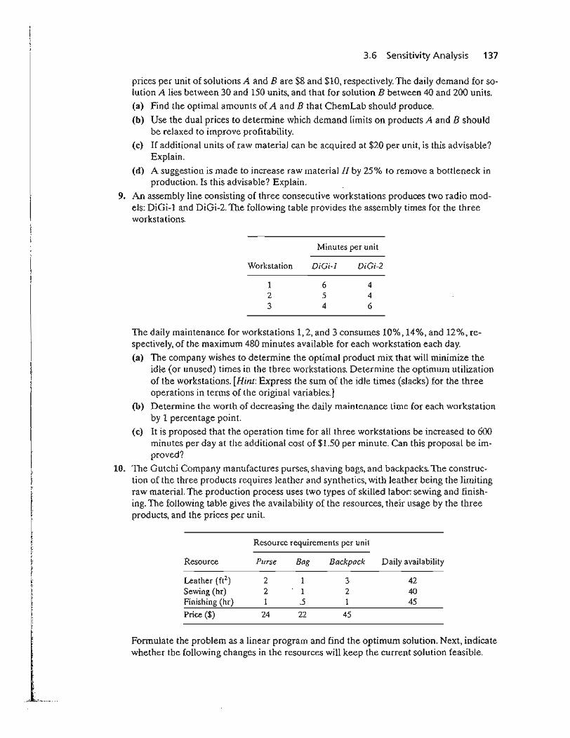
3.6 Sensitivity Analysis 137
prices per unit of solutions A and Bare $8 and $10, respectively. The daily demand for solution A lies between 30 and 150 units, and that for solution B between 40 and 200 units.(a) Find the optimal amounts of A and B that ChemLab should produce.
(b) Use the dual prices to determine which demand limits on products A and B shouldbe relaxed to improve profitability.
(c) If additional units of raw material can be acquired at $20 per unit, is this advisable?Explain.
(d) A suggestion is made to increase raw material II by 25% to remove a bottleneck inproduction. Is this advisable? Explain.
9. An assembly line consisting of three consecutive workstations produces two radio models: DiGi-l and DiGi-2. The following table provides the assembly times for the threeworkstations.
Minutes per unit
Workstation
123
DiGi-l
654
DiGi-2
446
The daily maintenance for workstations 1,2, and 3 consumes 10%,14%, and 12%, respectively, of the maximum 480 minutes available for each workstation each day.
(a) The company wishes to determine the optimal product mix that will minimize theidle (or unused) times in the three workstations. Determine the optimum utilizationof the workstations. [Hint; Express the sum of the idle times (slacks) for the threeoperations in terms of the original variables.]
(b) Determine the worth of decreasing the daily maintenance time for each workstationby 1 percentage point.
(c) It is proposed that the operation time for all three workstations be increased to 600minutes per day at the additional cost of $1.50 per minute. Can this proposal be improved?
10. The Gutchi Company manufactures purses, shaving bags, and backpacks. The construction of the three products requires leather and synthetics, with leather being the limitingraw material. The production process uses two types of skilled labor: sewing and finishing. The following table gives the availability of the resources, their usage by the threeproducts, and the prices per unit.
Resource requirements per unit
Resource Purse Bag Backpack Daily availability
Leather (ftZ) 2 1 3 42
Sewing (hr) 2 1 2 40Finishing (hr) 1 .5 1 45Price ($) 24 22 45
Formulate the problem as a linear program and find the optimum solution. Next, indicatewhether the following changes in the resources will keep the current solution feasible.
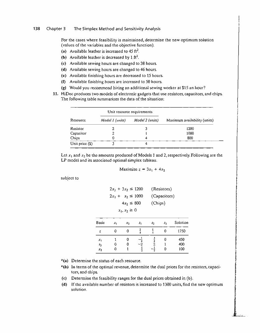
138 Chapter 3 The Simplex Method and Sensitivity Analysis
For the cases where feasibility is maintained, determine the new optimum solution(values of the variables and the objective function).
(a) Available leather is increased to 45 ft2•
(b) Available leather is decreased by 1 ft2•
(c) Available sewing hours are changed to 38 hours.
(d) Available sewing hours are changed to 46 hours.
(e) Available finishing hours are decreased to 15 hours.
(f) Available finishing hours are increased to 50 hours.
(g) Would you recommend hiring an additional sewing worker at $15 an hour?
11. HiDec produces two models of electronic gadgets that use resistors, capacitors, and chips.The following table summarizes the data of the situation:
Unit resource requirements
Resource
ResistorCapacitorChipsUnit price ($)
Modell (units)
22o3
Model 2 (units)
314
4
Maximum availability (units)
12001000800
Let Xt and X2 be the amounts produced of Models 1 and 2, respectively. Following are theLP model and its associated optimal simplex tableau.
Maximize z = 3X1 + 4X2
subject to
2xl + 3X2 :5 1200 (Resistors)
2x) + X2 :5 1000 (Capacitors)
4x2:::;; 800 (Chips)
Xl> X2 ;::: 0
Basic XI X2 Sl S2 S3 Solution
0 0 ~ I 0 1750z 4 4
x, 1 0 _1 ;! 0 4504 4
s3 0 0 -2 2 1 4000 1
, I 0 100X2 2 -2
*(a) Determine the status of each resource.
*(b) In terms of the optimal revenue, determine the dual prices for the resistors, capacitors, and chips.
(c) Determine the feasibility ranges for the dual prices obtained in (b).
(d) If the available number of resistors is increased to 1300 units, find the new optimumsolution.
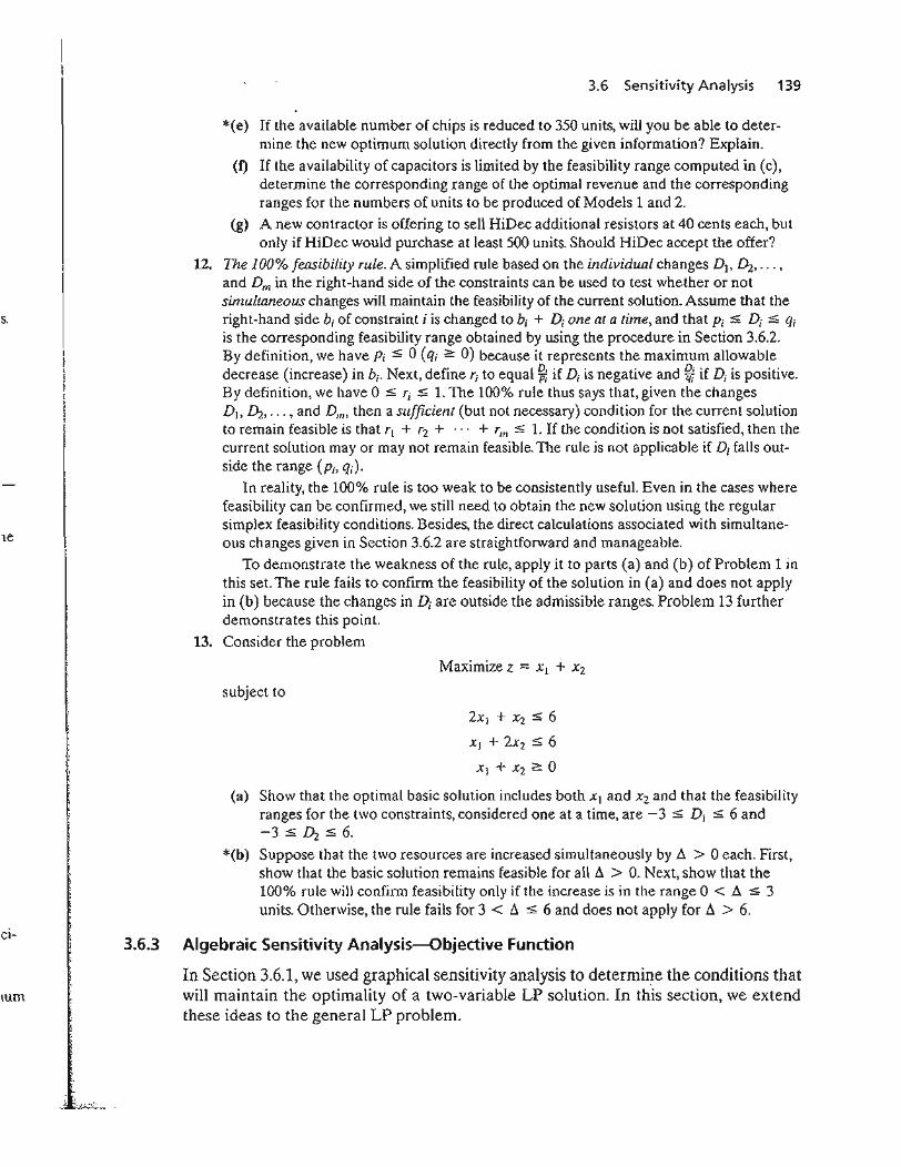
s.
ci-
lum
. 'i,.' '-~~:;:'__ .
3.6 Sensitivity Analysis 139
*(e) If the available number of chips is reduced to 350 units, will you be able to determine the new optimum solution directly from the given information? Explain.
(f) If the availability of capacitors is limited by the feasibility range computed in (c),determine the corresponding range of the optimal revenue and the correspondingranges for the numbers of units to be produced of Models 1 and 2.
(g) A new contractor is offering to sell HiDec additional resistors at 40 cents each, butonly if HiDec would purchase at least 500 units. Should HiDec accept the offer?
U. The 100% feasibility rule. A simplified rule based on the individual changes Db ~, ... ,and Dm in the right-hand side of the constraints can be used to test whether or notsimultaneous changes will maintain the feasibility of the current solution. Assume that theright-hand side bj of constraint i is changed to bi + D; one at a time, and that P; :::;; D; :::;; qjis the corresponding feasibility range obtained by using the procedure in Section 3.6.2.By definition, we have PI :::;; 0 (qj ~ 0) because it represents the maximum allowabledecrease (increase) in b;. Next, define'j to equal ~ if Dj is negative and!Jf if Dj is positive.By definition, we have 0 :::;; I"j :$ 1. The 100% rule thus says that, given the changesDb ~, ... , and Dm , then a sufficient (but not necessary) condition for the current solutionto remain feasible is that 1"1 + '2 + ... + rill :::;; 1. If the condition is not satisfied, then thecurrent solution mayor may not remain feasible. The rule is not applicable if Dj falls outside the range (Pj, q;).
In reality, the 100% rule is too weak to be consistently useful. Even in the cases wherefeasibility can be confirmed, we still need to obtain the new solution using the regularsimplex feasibility conditions. Besides, the direct calculations associated with simultaneous changes given in Section 3.6.2 are straightforward and manageable.
To demonstrate the weakness of the rule, apply it to parts (a) and (b) of Problem 1 inthis set. The rule fails to confirm the feasibility of the solution in (a) and does not applyin (b) because the changes in Dj arc outside the admissible ranges. Problem 13 furtherdemonstrates this point.
13. Consider the problem
Maximize z "" XI + X2
subject to
2Xl + X2 :$ 6
XI + 2X2 :::;; 6
Xl + X2 ~ 0
(a) Show that the optimal basic solution includes both Xl and X2 and that the feasibilityranges for the two constraints, considered one at a time, are - 3 ~ DI :OS 6 and-3 :::;; D2 :::;; 6.
*(b) Suppose that the two resources are increased simultaneously by 6. > 0 each. First,show that the basic solution remains feasible for all 6. > O. Next, show that the100% rule will confirm feasibility only if the increase is in the range 0 < A :$ 3units. Otherwise, the rule fails for 3 < Ii ~ 6 and does not apply for 6. > 6.
3.6.3 Algebraic Sensitivity Analysis-objective Function
In Section 3.6.1, we used graphical sensitivity analysis to determine the conditions thatwill maintain the optimality of a two-variable LP solution. In this section, we extendthese ideas to the general LP problem.
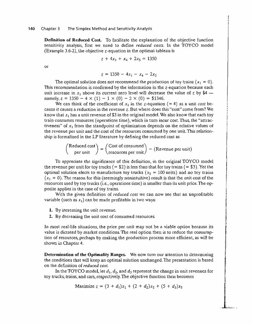
140 Chapter 3 The Simplex Method and Sensitivity Analysis
Definition of Reduced Cost. To facilitate the explanation of the objective functionsensitivity analysis, first we need to define reduced costs. In the TOYCO model(Example 3.6-2), the objective z-equation in the optimal tableau is
z + 4XI + X4 + 2x5 = 1350
or
z = 1350 - 4X1 - X4 - 2X5
The optimal solution does not recommend the production of toy trains (Xl = 0).This recommendation is confirmed by the informatIon in the z-equation because eachunit increase in Xl above its current zero level will decrease the value of z by $4 namely, z = 1350 - 4 X (1) - 1 x (0) - 2 X (0) = $1346.
We can think of the coefficient of xl in the z-equation (= 4) as a unit cost because it causes a reduction in the revenue z. But where does this "cost" come from? Weknow that xl has a unit revenue of $3 in the original model. We also know that each toytrain consumes resources (operations time), which in turn incur cost. Thus, the "attractiveness" of Xl from the standpoint of optimization depends on the relative values ofthe revenue per unit and the cost of the resources consumed by one unit. This relationship is formalized in the LP literature by defining the reduced cost as
(Reduced cost) (cost of consumed) (R . )= . - evenue per umt
per unit resources per umt
To appreciate the significance of this definition, in the original TOYCO modelthe revenue per unit for toy trucks (= $2) is less than that for toy trains (= $3). Yet theoptimal solution elects to manufacture toy trucks (X2 = 100 units) and no toy trains(XI = 0). The reason for this (seemingly nonintuitive) result is that the unit cost of theresources used by toy trucks (i.e., operations time) is smaller than its unit price. The opposite applies in the case of toy trains.
With the given definition of reduced cost we can now see that an unprofitablevariable (such as Xl) can be made profitable in two ways:
1. By increasing the unit revenue.
2. By decreasing the unit cost of consumed resources.
In most real-life situations, the price per unit may not be a viable option because itsvalue is dictated by market conditions. The real option then is to reduce the consumption of resources, perhaps by making the production process more efficient, as will beshown in Chapter 4.
Determination of the Optimality Ranges. We now turn our attention to determiningthe conditions that will keep an optimal solution unchanged. The presentation is basedon the definition of reduced cost.
In the TOYCO model, let db d2, and d3 represent the change in unit revenues fortoy trucks, trains, and cars, respectively. The objective function then becomes
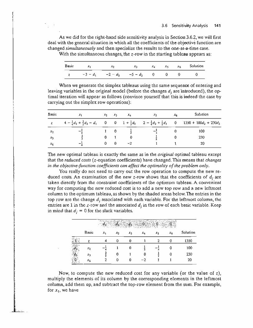
3.6 Sensitivity Analysis 141
As we did for the right-hand side sensitivity analysis in Section 3.6.2, we will firstdeal with the general situation in which all the coefficients of the objective function arechanged simultaneously and then specialize the results to the one-at-a-time case.
With the simultaneous changes, the z-row in the starting tableau appears as:
Basic
o o o
Solution
o
j
r
When we generate the simplex tableaus using the same sequence of entering andleaving variables in the original model (before the changes d j are introduced), the optimal iteration will appear as follows (convince yourself that this is indeed the case bycarrying out the simplex row operations):
Basic Xl X2 X3 X4 Xs X6 Solution
1 3 0 0 1 2 - 1d + 1d3 0 1350 + 100dl + 230d3Z 4 - 4dZ + "2d3 - d l 1 + "2dz 4 Z 1
1 1 0 I _1 0 100Xl -4 "2 43 0 1 0 I 0 230X3 "2 "2
X6_1 0 0 -2 1 204
The new optimal tableau is exactly the same as in the original optimal tableau exceptthat the reduced costs (z-equation coefficients) have changed. This means that changesin the objective-function coefficients can affect the optimality of the problem only.
You really do not need to carry out the row operation to compute the new reduced costs. An examination of the new z-row shows that the coefficients of dj aretaken directly from the constraint coefficients of the optimum tableau. A convenientway for computing the new reduced cost is to add a new top row and a new leftmostcolumn to the optimum tableau, as shown by the shaded areas below. The entries in thetop row are the change d j associated with each variable. For the leftmost column, theentries are 1 in the z-row and the associated dj in the row of each basic variable. Keepin mind that d j = 0 for the slack variables.
Basic Xl X2 X3 X4 X5 X6 Solution
:;;.'1[:) z 4 0 0 1 2 0 1350: ;.<;.:: ~ .•
_1 1 1
:i:~!~~X2 4 1 0 "2 -4 0 100
xJ2- 0 1 0 1 0 230z 2
),~:9;r x6 2 0 0 ~2 1 1 20
Now, to compute the new reduced cost for any variable (or the value of z),multiply the elements of its column by the corresponding elements in the leftmostcolumn, add them up, and subtract the top-row element from the sum. For example,for Xl, we have
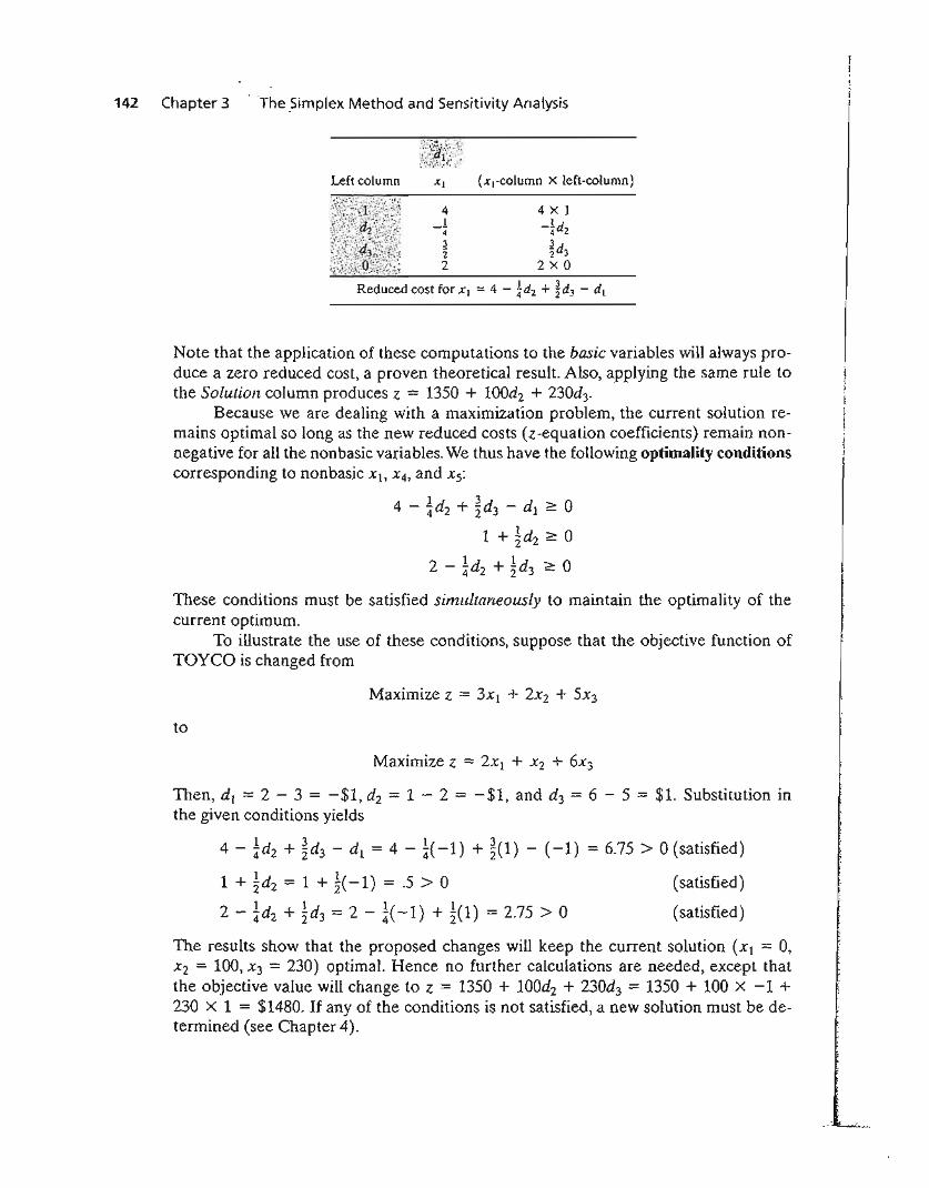
142 Chapter 3 . The Simplex Method and Sensitivity Analysis
Left column
;~~;~1Y:~:~;XI
4_1
4322
(xl-column X left·column)
4 X 1_ld
4 2
~d32xQ
Reduced cost for XI = 4 - ~d2 + ~d3 - d l
Note that the application of these computations to the basic variables will always produce a zero reduced cost, a proven theoretical result. Also, applying the same rule tothe Solution column produces z = 1350 + 100d2 + 230d3.
Because we are dealing with a maximization problem, the current solution remains optimal so long as the new reduced costs (z-equation coefficients) remain nonnegative for all the nonbasic variables. We thus have the following optimality conditionscorresponding to nonbasic Xb X4, and Xs:
4 - ~d2 + ~d3 - d1 ~ 0
1 + ~d2 ~ 01 1 02 - 4d2 + 2d3 ~
These conditions must be satisfied simultaneously to maintain the optimality of thecurrent optimum.
To illustrate the use of these conditions, suppose that the objective function ofTOYCO is changed from
Maximize z = 3Xl + 2X2 + 5X3
to
Maximize z = 2Xl + X2 + 6X3
Then, d} = 2 - 3 = -$1, d2 = 1 - 2 = -$1, and d3 = 6 - 5 = $1. Substitution inthe given conditions yields
4 - ~d2 + ~d3 - d 1 = 4 - ~(-1) + ~(1) - (-1) = 6.75 > 0 (satisfied)
1 + ~d2 = 1 + ~(-1) = .5 > 0 (satisfied) ~
2 - ~d2 + ~d3 = 2 - ~(-1) + !(1) = 2.75 > 0 (satisfied) f
The results show that the proposed changes will keep the current solution (Xl = 0, I·.:
X2 = 100, X3 = 230) optimal. Hence no further calculations are needed, except thatthe objective value will change to z = 1350 + 100d2 + 230d3 = 1350 + 100 X -1 +230 X 1 = $1480. If any of the conditions is not satisfied, a new solution must be determined (see Chapter 4).
_,:,"'~"".
e
III
0,lat
+le-
3.6 Sensitivity Analysis 143
The discussion so far has dealt with the maximization case. The only difference inthe minimization case is that the reduced costs (z-equations coefficients) must be ::;0to maintain optimality.
The general optimality conditions can be used to determine the special casewhere the changes dj occur one at a time instead of simultaneously. This analysis isequivalent to considering the following three cases:
1. Maximize z = (3 + dl)XI + 2xz + 5X3
2. Maximize z = 3Xl + (2 + dz)xz + 5x3
3. Maximize z = 3xI + 2xz + (5 + d3 )X3
The individual conditions can be accounted for as special cases of the simultaneous case.s
Case 1. Set dz = d3 = 0 in the simultaneous conditions, which gives
4 - dj ~ O:==}-oo < d l ::; 4
Case 2. Set dl = d3 = ain the simultaneous conditions, which gives
4 - ~dz ~ a=> dz <: 16 }1 + !dz ~ 0 => dz ~ -2 => - 2 ::; dz <: 8
2 - ~ dz ~ a=> dz -< 8
Case 3. Set d l = dz = 0 in the simultaneous conditions, which gives
The given individual conditions can be translated in terms of the total unit revenue. For example, for toy trucks (variable xz), the total unit revenue is 2 + dz and theassociated condition -2 ::; dz <: 8 translates to
2 + (-2) ::; 2 + dz :=:; 2 + 8
or
$0 ::; (Unit revenue of toy truck) ::; $10
This condition assumes that the unit revenues for toy trains and toy cars remain fixedat $3 and $5, respectively.
The allowable range ($0, $10) indicates that the unit revenue of toy trucks (variable xz) can be as low as $0 or as high as $10 without changing the current optimum,Xl = 0, X2 = 100, X3 = 230. The total revenue will change to 1350 + 100dz, however.
5nJe individual ranges are standard outputs in all LP software. Simultaneous conditions usually are not partof the output, presumably because they are cumbersome for large problems.
144 Chapte~ 3 The Simplex Method and Sensitivity Analysis
It is important to notice that the changes db dz, and d3 may be within their allowable individual ranges without satisfying the simultaneous conditions, and vice versa.For example, consider
Maximize z = 6x} + 8xz + 3X3
Here d1 = 6 - 3 = $3, dz = 8 - 2 = $6, and d3 = 3 - 5 = -$2, which are allwithin the permissible individual ranges (- 00 < d 1 $ 4, -2 $ d2 <: 8, and-~ $ d3 < (0). However, the corresponding simultaneous conditions yield
4 - ~d2 + ~d3 - d1 = 4 - i(6) + ~(-2) - 3 = -3.5 < 0 (not satisfied)
1 + ~d2 = 1 + ~(6) = 4 > 0 (satisfied)
2 - id2 + ~d3 = 2 - ~(6) + ~(-2) = -.5 < 0 (not satisfied)
The results above can be summarized as follows:
1. The optimal values of the variables remain unchanged so long as the changesd j , j = 1, 2, ... , n, in the objective function coefficients satisfy all the optimalityconditions when the changes are simultaneous or fall within the optimalityranges when a change is made individually_
2. For other situations where the simultaneous optimality conditions are not satisfied or the individual feasibility ranges are violated, the recourse is to either resolve the problem with the new values of dj or apply the post-optimal analysispresented in Chapter 4.
PROBLEM SET 3.606
1. In the TOYCO model, determine if the current solution will change in each of the following cases:
(i) Z = 2Xl + X2 + 4X3
(ii) Z = 3xl + 6X2 + X3
(iii) z = 8Xl + 3X2 + 9x)
*2. B&K grocery store sells three types of soft drinks: the brand names Al Cola and A2 Colaand the cheaper store brand BK Cola. The price per can for Al, A2, and BK are 80, 70,and 60 cents, respectively. On the average, the store sells no more than 500 cans of allcolas a day. Although Al is a recognized brand name, customers tend to buy more A2and BK because they are cheaper. It is estimated that at least 100 cans of Al are solddaily and that A2 and BK combined outsell Al by a margin of at least 4:2.
(a) Show that the optimum solution does not call for selling the A3 brand.
(b) By how much should the price per can of A3 be increased to be sold by B&K?
(c) To be competitive with other stores, B&K decided to lower the price on all threetypes of cola by 5 cents per can. Recompute the reduced costs to determine if thispromotion will change the current optimum solution.
61n this problem set, you may find it convenient to generate the optimal simplex tableau with TORA.
3.6 Sensitivity Analysis 145
3. Baba Furniture Company employs four carpenters for 10 days to assemble tables andchairs. It takes 2 person-hours to assemble a table and .5 person-hour to assemble a chair.Customers usually buy one table and four to six chairs. The prices are $135 per table and$50 per chair. The company operates one 8-hour shift a day.
(a) Determine the 10-day optimal production mix.(b) If the present unit prices per table and chair are each reduced by 10%, use sensitivi
ty analysis to determine if the optimum solution obtained in (a) will change.
(c) If the present unit prices per table and chair are changed to $120 and $,25, will thesolution in (a) change?
4. The Bank of Elkins is allocating a maximum of $200,000 for personal and car loans during the next month. The bank charges 14% for personal loans and 12% for car loans.Both types of loans are repaid at the end of a I-year period. Experience shows that about3% of personal loans and 2% of car loans are not repaid. The bank usually allocates atleast twice as much to car loans as to personal loans.
(a) Determine the optimal allocation of funds between the two loans and the net rate ofreturn on all the loans.
(b) If the percentages of personal and car loans are changed to 4% and 3%, respectively,use sensitivity analysis to determine jf the optimum solution in (a) will change.
*5. Electra produces four types of electric motors, each on a separate assembly line. The respective capacities of the lines are 500, 500, 800, and 750 motors per day. Type 1 motoruses 8 units of a certain electronic component, type 2 motor uses 5 units, type 3 motoruses 4 units, and type 4 motor uses 6 units. The supplier of the component can provide8000 pieces a day. The prices per motor for the respective types are $60, $40, $25, $30.
(a) Determine the optimum daily production mix.
(b) The present production schedule meets Electra's needs. However, because of competition, Electra may need to lower the price of type 2 motor. What is the most reduction that can be effected without changing the present production schedule?
(c) Electra has decided to slash the price of all motor types by 25%. Use sensitivityanalysis to determine if the optimum solution remains unchanged.
(d) Currently, type 4 motor is not produced. By how much should its price be increasedto be induded in the production schedule?
6. Popeye Canning is contracted to receive daily 60,000 lb of ripe tomatoes at 7 cents perpound from which it produces canned tomato juice, tomato sauce, and tomato paste. Thecanned products are packaged in 24-can cases. A can of juice uses lib of fresh tomatoes,a can of sauce uses ~ lb, and a can of paste uses ~ lb. TIle company's daily share of themarket is limited to 2000 cases of juice, 5000 cases of sauce, and 6000 cases of paste. Thewholesale prices per case of juice, sauce, and paste are $21, $9, and $12, respectively.
(a) Develop an optimum daily production program for Popeye.
(b) If the price per case for juice and paste remains fixed as given in the problem, usesensitivity analysis to determine the unit price range Popeye should charge for a caseof sauce to keep the optimum product mix unchanged.
7. Dean's Furniture Company assembles regular and deluxe kitchen cabinets from precutlumber. The regular cabinets are painted white, and the deluxe are varnished. Both painting and varnishing are carried out in one department. TIle daily capacity of the assemblydepartment is 200 regular cabinets and 150 deluxe. Varnishing a deluxe unit takes twiceas much time as painting a regular one. If the painting/varnishing department is dedicated to the deluxe units only, it can complete 180 units daily. The company estimates thatthe revenues per unit for the regular and deluxe cabinets are $100 and $140, respectively.
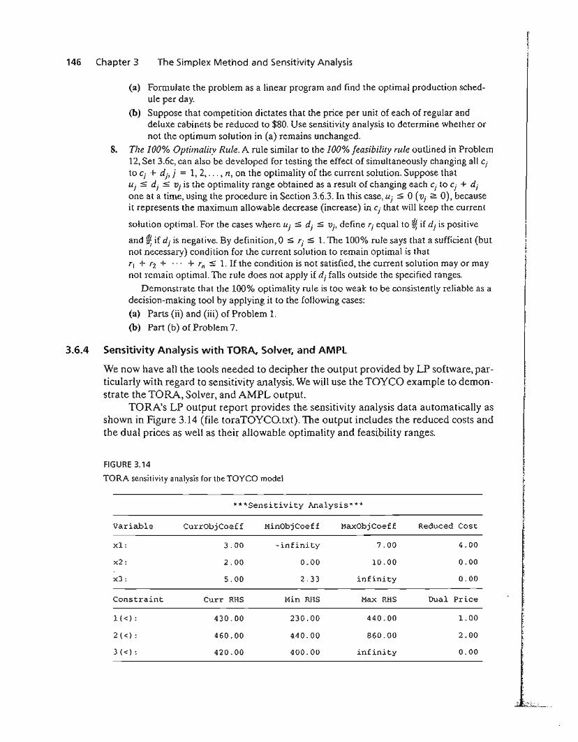
146 Chapter 3 The Simplex Method and Sensitivity Analysis
(a) Formulate the problem as a linear program and find the optimal production schedule per day.
(b) Suppose that competition dictates that the price per unit of each of regular anddeluxe cabinets be reduced to $80. Use sensitivity analysis to determine whether ornot the optimum solution in (a) remains unchanged.
8. The 100% Optimality Rule. A rule similar to the 100% feasibility rule outlined in Problem12, Set 3.6c, can also be developed for testing the effect of simultaneously changing all Cj
to Cj + dj , j := 1,2, ... , n, on the optimality of the current solution. Suppose thatUj :s d j :s Vj is the optimality range obtained as a result of changing each Cj to Cj + d j
one at a time, using the procedure in Section 3.6.3. In this case, Uj 5 0 (Vj ~ 0), becauseit represents the maximum allowable decrease (increase) in Cj that will keep the current
solution optimal. For the cases where Uj :s dj ::5 Vj. define Tj equal to ~ if dj is positive
and ~ if dj is negative. By definition, 0 ::5 rj ::5 1. The 100% rule says that a sufficient (butnot necessary) condition for the current solution to remain optimal is thatT\ + 1"2 + ... + Til ::5 1. If the condition is not satisfied, the current solution mayor maynot remain optimal.111e rule does not apply if dj falls outside the specified ranges.
Demonstrate that the 100% optimality rule is too weak to be consistently reliable as adecision-making tool by applying it to the following cases:
(a) Parts (ii) and (iii) of Problem 1.
(b) Part (b) of Problem 7.
3.6.4 Sensitivity Analysis with TORA, Solver, and AMPL
We now have all the tools needed to decipher the output provided by LP software, particularly with regard to sensitivity analysis. We will use the TOYCO example to demonstrate the TORA, Solver, and AMPL output.
TORA's LP output report provides the sensitivity analysis data automatically asshown in Figure 3.14 (file toraTOYCO.txt). The output includes the reduced costs andthe dual prices as well as their allowable optimality and feasibility ranges.
FIGURE 3.14
TORA sensitivity analysis for the TOYCO model
***Sensitivity Analysis***
Variable CurrObjCoeff MinObjCoeff MaxObjCoeff
xl: 3.00 -infinity 7.00
x2: 2.00 0.00 10.00
x3: 5.00 2.33 infinity
constraint Curr RHS Min RHS Max RHS
1 «): 430.00 230.00 440.00
2 «) : 460.00 440.00 860.00
3 «) : 420.00 400.00 infinity
Reduced Cost
4.00
0.00
0.00
Dual Price
1. 00
2.00
0.00
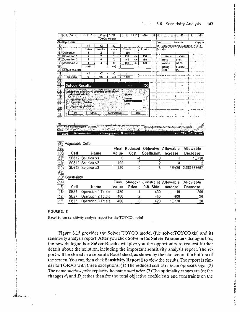
3.6 Sensitivity Analysis 147
00 iC2::J In ut data: . Cell: formula Copy to'>3;, x1 x2 x3.!. : E~· '.SUIJPP.OOUCT(BS:05,BS12:0SI2 E£:E8
::i;~Ob'ec'ive lra~ns!rut a;rs !:·!~!-J~i.iS.~r:-~;i:i·i:~E5-·-····. --'--'--",'" ._..
pi::;,6:";j-'O;.t:.:e:.:.:ra:.;ti;.::.an:.:..,;-1--I-_-=1_+----=2_+----=-1_;-~;-.;-:..+-~4='=30~-+<~:.~-: flome Celis.'::!J!.' 0 aralian 2 3 0 2 460 ! ~."-~.9~ E,,:,E.B._ .. J
··.S:,:, Operation 3 1 4 0 420 . .. ~~~.~~~.~ ~:.~~ _ .. ... _.:i'9tj >-0 >-0 : luti.n.. B.12:012
.'~O· Ou ul results: proll E~· "
~~:--·soiu·tio'ri-I ~1 l~O 2;30 1:S0 j~ i-·-· ..· .. +_.+-1-__ .._. __ ~..... n __ • -::-.: ·:i'~~:~··:1~'3.~ i I _;I:"'~. ~- ~~.l~.:-:.l'.~:·.~~::.:·::::~;,.-.~:-~.·.-.~~.' ·_·~~,;,i._~~~-_·...!- ...'~.' ~~li'~ .. ~.
r2~~ I!J§~l?~~'~';~":~,?"TrH>_f~~~1-;'"l' e:r....; l..' '" ' I. • ..•~.: •.L L .~__ ._.~ ___.__.~ ..._....~..... .,'. ~ .__.;~~ 'i{~.:·~r::'TT'''~~4·:~T;·{. Sa:~~.nario 1'( t!~p .1·. "'n.. " .
$8$12 Solution x1$C$12 Solution x2
Cell ttame
SDS12 Solution x3
1E+302
AllowableDecrease
2.666666667
o -4 3 4
230 0 51E+30100 0 2 B
Final Reduced Objective AllowableValue Cost Coefficient Increase
Final Shadow Constraint Allowable AllowableValue Price R.H. Side Increase Decrease
430 1 430 10 200460 2 460 400 20400 0 420 lE+30 20
Name
Operation 3 TotalsOperation 2 TotalsOperation 1 Totals
Cell
$ES8
$ESE$ES7
A~~ Adjustable Cells::i:~-~~~·::
~~~::jit9Y.(~J>:
i1.l;,;}2:;~;j~i Constraints
Ak)~..:
;1$:in:,.18"
.sd
FIGURE 3.15
Excel Solver sensitivity analysis report for the TOYCO model
Figure 3.15 provides the Solver TOYCO model (file solverTOYCo.xls) and itssensitivity analysis report. After you click Solve in the Solvcr Parameters dialogue box,the new dialogue box Solver Rcsults will give you the opportunity to request furtherdetails about the solution, including the important sensitivity analysis report. The report will be stored in a separate Excel sheet, as shown by the choices on the bottom ofthe screen. You can then click Sensitivity Report 1 to view the results. The report is similar to TORA's with three exceptions: (1) The reduced cost carries an opposite sign. (2)The name shadow price replaces the name du.al price. (3) The optimality ranges are for thechanges dj and D j rather than for the total objective coefficients and constraints on the
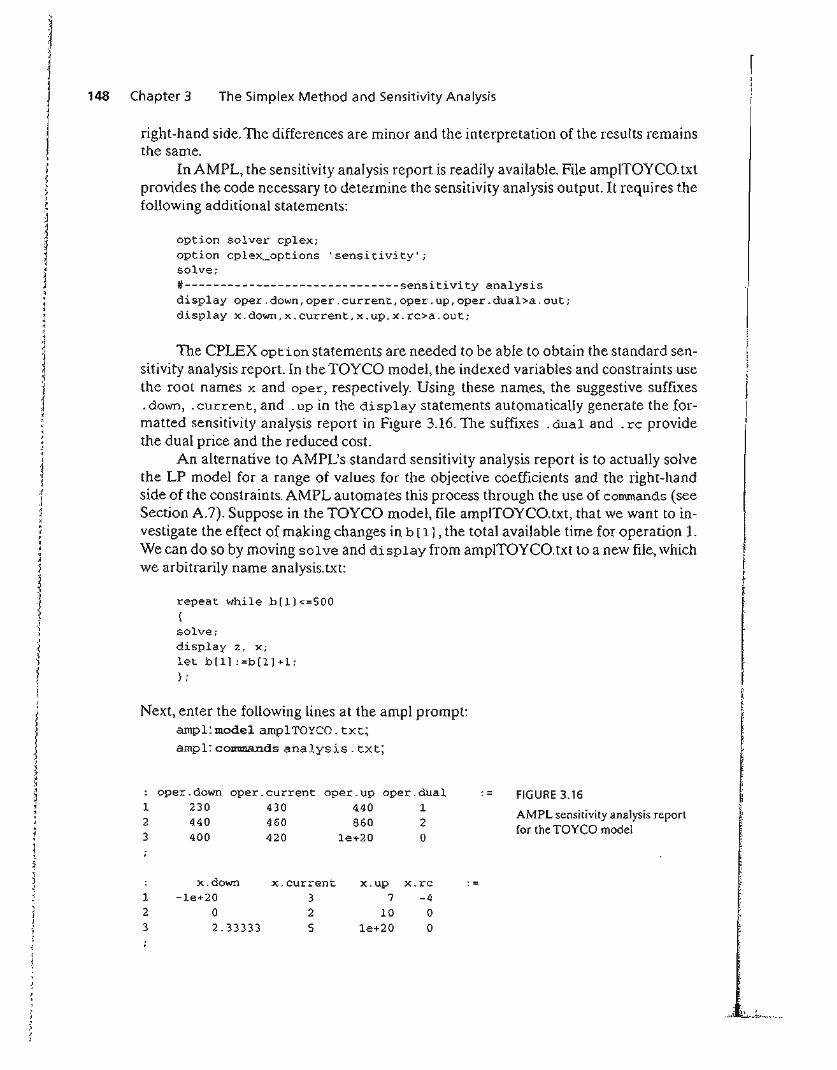
right-hand side. The differences are minor and the interpretation of the results remainsthe same.
In AMPL, the sensitivity analysis report is readily available. File amplTOYCo.txtprovides the code necessary to determine the sensitivity analysis output. It requires thefollowing additional statements:
11
~
1
I.,148 Chapter 3 The Simplex Method and Sensitivity Analysis
option solver cplex;option cplex_options 'sensitivity';solve;#------------------------------sensitivity analysisdisplay oper.down,oper.current,oper.up,oper.dual>a.out;display x.down,x.current,x.up,x.rc>a.out;
repeat while b[ll<=500{
solve;display z, X;let b[l] :=b[l]+l;} ;
The CPLEX option statements are needed to be able to obtain the standard sensitivity analysis report. In the TOYCO model, the indexed variables and constraints usethe root names x and oper, respectively. Using these names, the suggestive suffixes. down, . current, and. up in the display statements automatically generate the formatted sensitivity analysis report in Figure 3.16. The suffixes .dual and. rc providethe dual price and the reduced cost.
An alternative to AMPL's standard sensitivity analysis report is to actually solvethe LP model for a range of values for the objective coefficients and the right-handside of the constraints. AMPL automates this process through the use of commands (seeSection A.7). Suppose in the TOYCO model, file amplTOYCo.txt, that we want to investigate the effect of making changes in b [1] , the total available time for operation l.We can do so by moving solve and display from amplTOYCO.txt to a new file, whichwe arbitrarily name analysis. txt:
Next, enter the following lines at the ampl prompt:ampl: model amplTOYCO. txt;
ampl: commands analysis. txt;
AMPL sensitivity analysis reportfor the TOyeD model
FIGURE 3.16oper.dual12o
oper.up440860
le+20
oper.current430460420
oper.down230440400
123
x.down x.current X.up x.rc :=
1 -le+20 3 7 -42 0 2 10 03 2.33333 5 le+20 0
3.6 Sensitivity Analysis 149
The first line will provide the model and its data and the second line will provide theoptimum solutions starting with b [II at 430 (the initial value given in amplTOYCO.txt)and continuing in increments of 1 until b [1] reaches 500. An examination of the output will then allow us to study the sensitivity of the optimum solution to changes inb [1 J•Similar procedures can be followed with other coefficients including the case ofmaking simultaneous changes.
PROBLEM SET 3.6eJ
1. Consider Problem 1, Set 2.3c (Chapter 2). Use the dual price to decide if it is worthwhileto increase the funding for year 4.
2. Consider Problem 2, Set 2.3c (Chapter 2).
(a) Use the dual prices to determine the overall return on investment.
(b) If you wish to spend $1000 on pleasure at the end of year 1, how would this affectthe accumulated amount at the start of year 5?
3. Consider Problem 3, Set 2.3c (Chapter 2).
(a) Give an economic interpretation of the dual prices of the model.
(b) Show how the dual price associated with the upper bound on borrowed money atthe beginning of the third quarter can be derived from the dual prices associatedwith the balance equations representing the in-out cash flow at the five designateddates of the year.
4. Consider Problem 4, Set 2.3c (Chapter 2). Use the dual prices to determine the rate of return associated with each year.
*5. Consider Problem 5, Set 2.3c (Chapter 2). Use the dual price to determine if it is worthwhile for the executive to invest more money in the plans.
6. Consider Problem 6, Set 2.3c (Chapter 2). Use the dual price to decide if it is advisablefor the gambler to bet additional money.
7. Consider Problem 1, Set 2.3d (Chapter 2). Relate the dual prices to the unit productioncosts of the model.
8. Consider Problem 2, Set 2.3d (Chapter 2). Suppose that any additional capacity of machines 1 and 2 can be acquired only by using overtime. What is the maximum cost perhour the company should be willing to incur for either machine?
*9. Consider Problem 3, Set 2.3d (Chapter 2).
(a) Suppose that the manufacturer can purchase additional units of raw material A at$12 per unit. Would it be advisable to do so?
(b) Would you recommend that the manufacturer purchase additional units of raw material B at $5 per unit?
10. Consider Problem 10, Set 2.3e (Chapter 2).
(a) Which of the specification constraints impacts the optimum solution adversely?
(b) What is the most the company should pay per ton of each ore?
7Before answering the problems in this set, you are expected to generate the sensitivity analysis report usingAMPL, Solver, orTORA.
150 Chapter 3
REFERENCES
The Simplex Method and Sensitivity Analysis
Bazaraa, M., 1. Jarvis, and H. Sherali, Linear Programming and Network Flows, 2nd ed., Wiley,New York, 1990.
Dantzig, G., Linear Programming and Extensions, Princeton University Press, Princeton,NJ,1963.
Dantzig, G., and M. Thapa, Linear Programming 1: Introduction, Springer, New York, 1997.
Fourer, R., D. Gay, and B. Kemighan, AMPL,A Modeling Language for Mathematical Programming, 2nd ed., Brooks/Cole-Thompson, Pacific Grove, CA, 2003.
Nering, E., and A. Thcker, Linear Programming and Related Problems, Academic Press, Boston,1992.
Schrage, L., Optimization Modeling with LINGO, LINDO Systems, Inc., Chicago, 1999.
Taha, H., "Linear Programming," Chapter II-l in Handbook of Operations Research, 1. Moderand S. Elmaghraby (eds.), Van Nostrand Reinhold, New York, 1987.
Il
, .'~ ::~~~
CHAPTER 4
Duality and Post-OptimalAnalysis
Chapter Guide. Chapter 3 dealt with the sensitivity of the optimal solution by determining the ranges for the model parameters that will keep the optimum basic solutionunchanged. A natural sequel to sensitivity analysis is post-optimal analysis, where thegoal is to determine the new optimum that results from making targeted changes in themodel parameters. Although post-optimal analysis can be carried out using the simplextableau computations in Section 3.6, this chapter is based entirely on the dual problem.
At a minimum, you will need to study the dual problem and its economic interpretation (Sections 4.1,4.2, and 4.3). The mathematical definition of the dual problem inSection 4.1 is purely abstract. Yet, when you study Section 4.3, you will see that the dualproblem leads to intriguing economic interpretations of the LP model, including dualprices and reduced costs. It also provides the foundation for the development of the newdual simplex algorithm, a prerequisite for post-optimal analysis. The dual simplex algorithm is also needed for integer programming in Chapter 9.
The generalized simplex algorithm in Section 4.4.2 is intended to show that thesimplex method is not rigid, in the sense that you can modify the rules to handle problems that start both infeasible and nonoptimal. However, this material may be skippedwithout loss of continuity.
You may use TORA's interactive mode to reinforce your understanding of thecomputational details of the dual simplex method.
This chapter includes 14 solved examples, 56 end-of-section problems, and 2cases. The cases are in Appendix E on the CD.
4.1 DEFINITION OF THE DUAL PROBLEM
The dual problem is an LP defined directly and systematically from the primal (or original) LP model. The two problems are so closely related that the optimal solution ofone problem automatically provides the optimal solution to the other.
In most LP treatments, the dual is defined for various forms of the primal depending on the sense of optimization (maximization or minimization), types of constraints
151
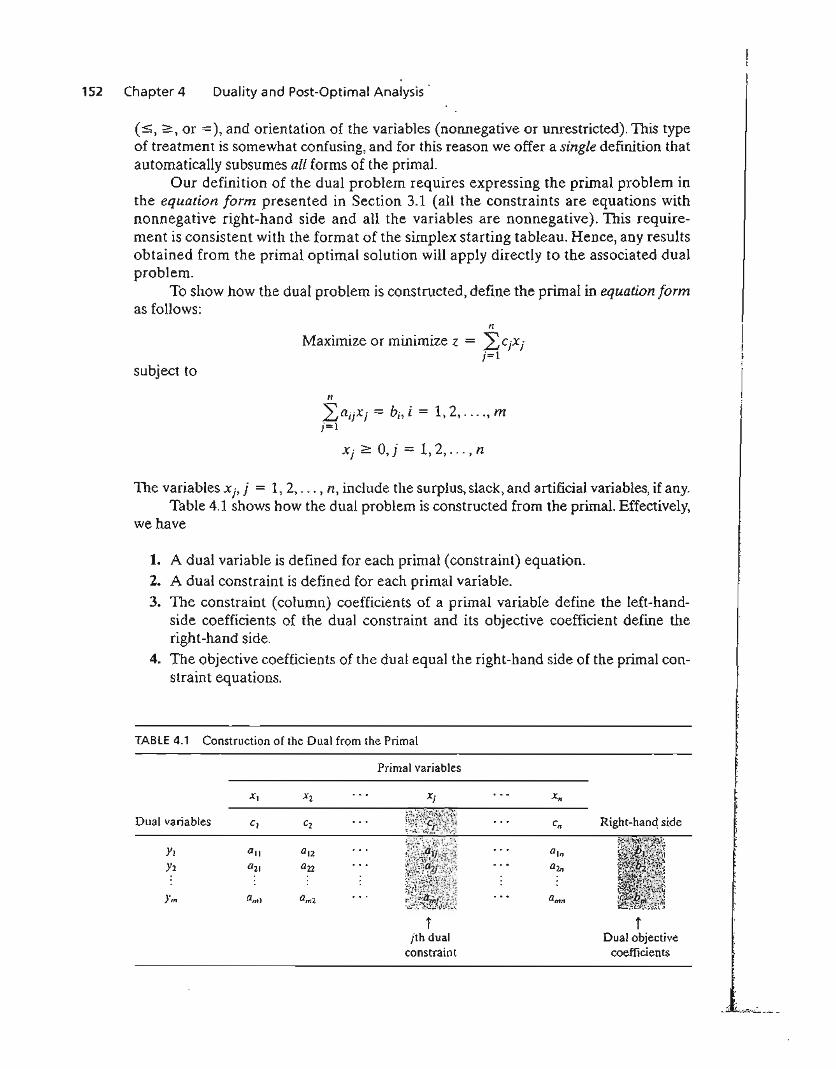
152 Chapter 4 Duality and Post-Optimal Analysis
(:5, ~, or =), and orientation of the variables (nonnegative or unrestricted). This typeof treatment is somewhat confusing, and for this reason we offer a single definition thatautomatically subsumes all forms of the primal.
Our definition of the dual problem requires expressing the primal problem inthe equation form presented in Section 3.1 (all the constraints are equations withnonnegative right-hand side and all the variables are nonnegative). This requirement is consistent with the format of the simplex starting tableau. Hence, any resultsobtained from the primal optimal solution will apply directly to the associated dualproblem.
To show how the dual problem is constructed, define the primal in equation formas follows:
n
Maximize or minimize z = 2>jXjj=l
subject to
tI
Lajjxj = bi , i = 1,2, ...., mj=l
Xj ;:::: 0, j = 1, 2, ... , n
The variables Xj' j = 1,2, ... , n, include the surplus, slack, and artificial variables, if any.Table 4.1 shows how the dual problem is constructed from the primal. Effectively,
we have
1. A dual variable is defined for each primal (constraint) equation.2. A dual constraint is defined for each primal variable.3. The constraint (column) coefficients of a primal variable define the left-hand
side coefficients of the dual constraint and its objective coefficient define theright-hand side.
4. The objective coefficients of the dual equal the right-hand side of the primal constraint equations.
TABLE 4.1 Construction of the Dual from the Primal
Primal variables
Xl x2
Dual variables CI C2
Yl all GI2
Y2 a21 an
Ym aml Qm2
tjth dual
constraint
Right-hand side
tDual objective
coefficients
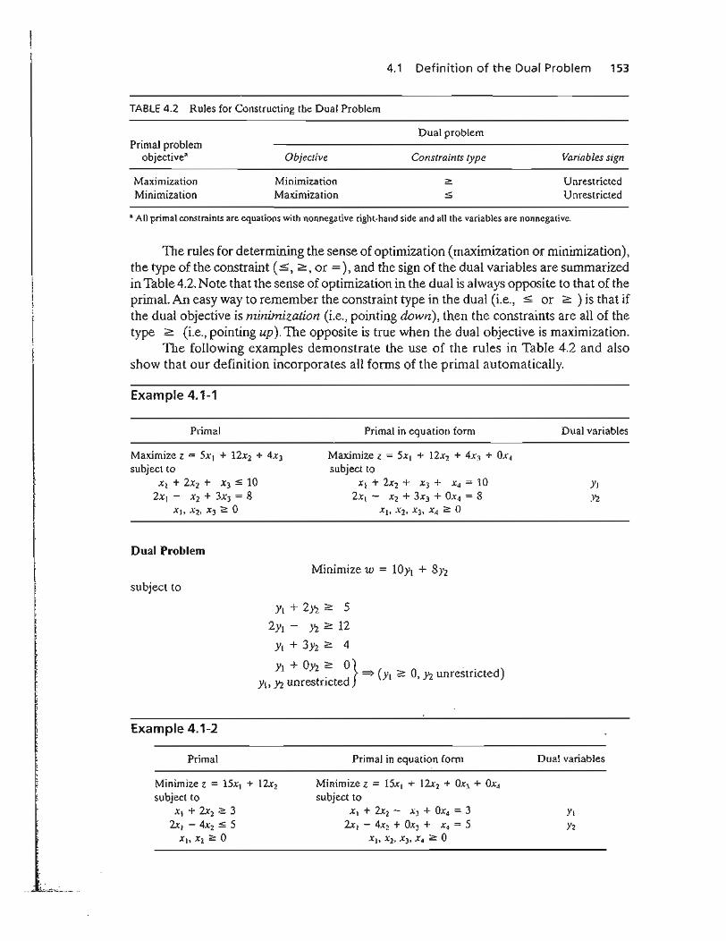
4.1 Defin ition of the Dual Problem 153
TABLE 4.2 Rules for Constructing the Dual Problem
Primal problemobjective"
MaximizationMinimization
Objective
MinimizationMaximization
Dual problem
Constraints type Variables sign
UnrestrictedUnrestricted
a All primal constraints are equations with nonnegative right-hand side and all the variables are nonnegative.
The rules for determining the sense of optimization (maximization or minimization),the type of the constraint (:s;, 2::, or =), and the sign of the dual variables are summarizedin Table 4.2. Note that the sense of optimization in the dual is always opposite to that of theprimal. An easy way to remember the constraint type in the dual (i.e., :s or 2:: ) is that ifthe dual objective is minimization (i.e., pointing down), then the constraints are all of thetype 2:: (i.e., pointing up). The opposite is true when the dual objective is maximization.
The following examples demonstrate the use of the rules in Table 4.2 and alsoshow that our definition incorporates all forms of the primal automatically.
Example 4.1-1
Primal
Maximize z = 5xI + 12x2 + 4X3
subject toXt + 2X2 + x3:5 10
2x, - X2 + 3X3 = 8XI> X2, X3 2 0
Dual Problem
subject to
Primal in equation form
Maximize z = 5XI + 12x2 + 4xJ + OX4subject to
Xl + 2X2 + X3 + X4 = 102xI - X2 + 3X3 + OX4 = 8
XI> X2. X3, X4 2 0
Minimize w = lOYl + 8Y2
Dual variables
Y.}'z
y, + 2yz ~ 5
2Yl - .Y2 ~ 12
Yt + 3yz ~ 4
Yl + Oyz ~ O} .. d => (Yt ;::: 0, Yz unrestricted)
Yt, Yz unrestncte
Example 4.1-2
Primal
Minimize z = 15x\ + 12x2subject to
XI + 2x2 232x1 - 4X2 :5 5
XI> X2 2 0
Primal in equation form
Minimize z = 15xl + 12x2 + OX3 + OX4
subject toXl + 2x2 - x) + OX4 = 3
2x1 - 4X2 + Ox) + X4 = 5Xl> X2, X3. X4 2 0
Dual variables
YI)'2
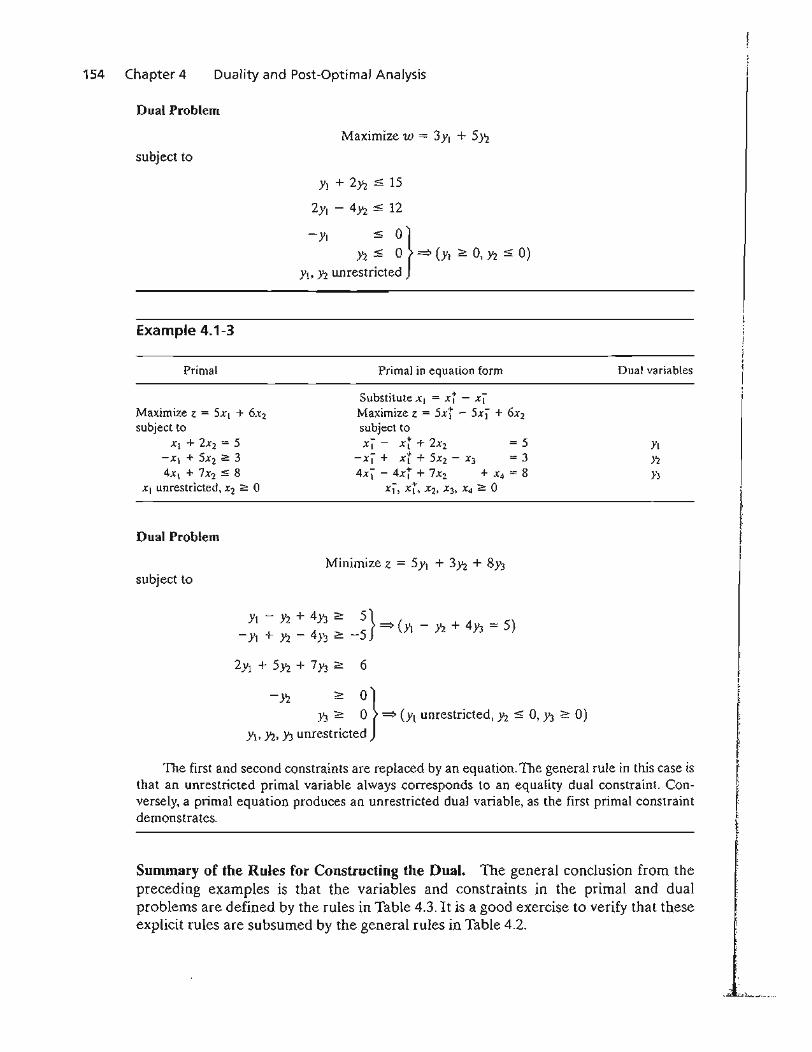
154 Cha pter 4 Duality and Post-Optimal Analysis
Dual Problem
Maximize w = 3 Y1 + 5)1
subject to
YI + 2)1 :5 15
2YI - 4)1 :5 12
-YI :5 O}Y2:5 0 ~ (Yl ~ 0, )1 :5 0)
Yl, Y2 unrestricted
Example 4.1-3
Primal
Maximize z = 5x[ + 6X2subject to
XJ + 2X2 = 5-XI + 5X2 ~ 34Xl + 7X2 =:; 8
xI unrestricted, x2 2: 0
Dual Problem
subject to
Primal in equation form
Substitute XI = xi - XIMaximize z = 5xi - 5xI + 6X2subject toXl - xi + 2X2 = 5
-Xl + xi + 5X2 - X3 = 34xI - 4xi + 7X2 + X4 = 8
XI, xl. X2, X3, X4 ~ 0
Minimize z = 5Yl + 3)1 + 8Y3
Dual variables
YI>'2Y3
-)1 ~ O})'3 ~ 0 ~ (Yl unrestricted, Yz :5 0')'3 ~ 0)
Yl, )1, )'3 unrestricted
The first and second constraints are replaced by an equation. The general rule in this case isthat an unrestricted primal variable always corresponds to an equality dual constraint. Conversely, a primal equation produces an unrestricted dual variable, as the first primal constraintdemonstrates.
Summary of the Rules for Constructing the Dual. The general conclusion from thepreceding examples is that the variables and constraints in the primal and dualproblems are defined by the rules in Table 4.3. It is a good exercise to verify that theseexplicit rules are subsumed by the general rules in Table 4.2.
"'~~..j"--'"
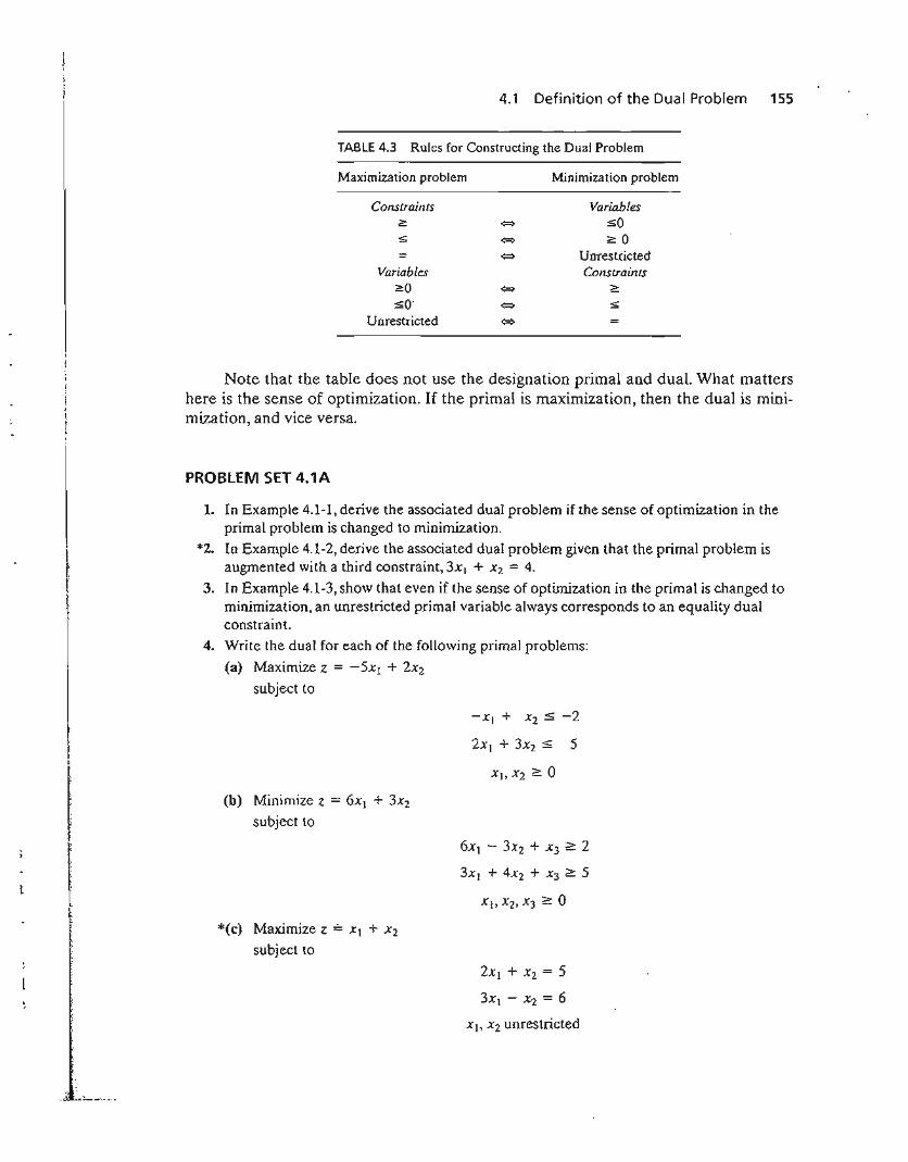
4.1 Definition of the Dual Problem 155
TABLE 4.3 Rules for Constructing the Dual Problem
Maximization problem
Constraints
Variables~O
.saUnrestricted
Minimization problem
VarUlbles.sO~O
UnrestrictedCOllStraints
f
If•t~I'
t~
"'::"'-~"--'"
Note that the table does not use the designation primal and dual. What mattershere is the sense of optimization. If the primal is maximization, then the dual is minimization, and vice versa.
PROBLEM SET 4.1A
1. In Example 4.1-1, derive the associated dual problem if the sense of optimization in theprimal problem is changed to minimization.
*2. In Example 4.1-2, derive the associated dual problem given that the primal problem isaugmented with a third constraint, 3Xl + X2 = 4.
3. In Example 4.1-3, show that even if the sense of optimization in the primal is changed tominimization, an unrestricted primal variable always corresponds to an equality dualconstraint.
4. Write the dual for each of the following primal problems:
(a) Maximize z = -5x[ + 2x2
subject to
-XI + x2:5-2
2Xl + 3X2:5 5
(b) Minimize z = 6x} + 3X2
subject to
6Xl - 3X2 + X3 ;;:: 2
3x[ + 4X2 + X3 2: 5
*(c) Maximize z == Xl + X2
subject to
2x[ + X2 = 5
3Xl - X2 = 6
Xl> X2 unrestricted
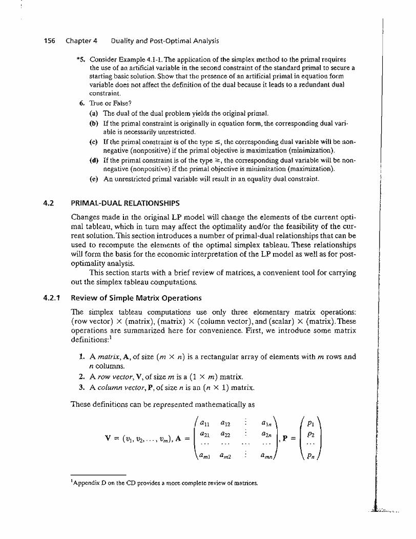
156 Chapter 4 Duality and Post-Optimal Analysis
*5. Consider Example 4.1-1. The application of the simplex method to the primal requiresthe use of an artificial variable in the second constraint of the standard primal to secure astarting basic solution. Show that the presence of an artificial primal in equation formvariable does not affect the definition of the dual because it leads to a redundant dualconstraint.
6. True or False?
(a) The dual of the dual problem yields the original primal.
(b) If the primal constraint is originally in equation form, the corresponding dual variable is necessarily unrestricted.
(c) If the primal constraint is of the type :5, the corresponding dual variable will be nonnegative (nonpositive) if the primal objective is maximization (minimization).
(d) If the primal constraint is of the type ;:::, the corresponding dual variable will be nonnegative (nonpositive) if the primal objective is minimization (maximization).
(e) An unrestricted primal variable will result in an equality dual constraint.
4.2 PRIMAL-DUAL RELATIONSHIPS
Changes made in the original LP model will change the elements of the current optimal tableau, which in turn may affect the optimality and/or the feasibility of the current solution.This section introduces a number of primal-dual relationships that can beused to recompute the elements of the optimal simplex tableau. These relationshipswill form the basis for the economic interpretation of the LP model as well as for postoptimality analysis.
This section starts with a brief review of matrices, a convenient tool for carryingout the simplex tableau computations.
4.2.1 Review of Simple Matrix Operations
The simplex tableau computations use only three elementary matrix operations:(row vector) X (matrix), (matrix) x (column vector), and (scalar) X (matrix).Theseoperations are summarized here for convenience. First, we introduce some matrixdefinitions:1
1. A matrix, A, of size (m X n) is a rectangular array of elements with m rows andn columns.
2. A row vector, V, of size m is a (1 X m) matrix.3. A column vector, P, of size n is an (n xl) matrix.
These definitions can be represented mathematically as
au a12 aln PI
V = (VI> V2, .. ·, v m), A = aZI a22 a2n p= pz,
amI a m2 a mn Pn
1Appendix 0 on the CO provides a more complete review of matrices.
'-;'.:''l'".• ::..:,.;.. __
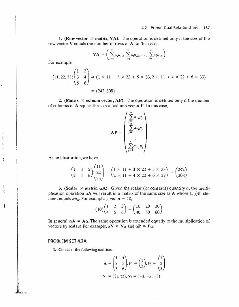
4.2 Primal-Dual Relationships 157
1. (Row vector X matrix, VA). The operation is defined only if the size of therow vector V equals the number of rows of A. In this case,
For example,
(11,22,33)0 ~) = (1 x 11 + 3 X 22 + 5 X 33,2 X 11 + 4 x 22 + 6 X 33)6 .
= (242,308)
2. (Matrix X column vector, AP). The operation is defined only if the numberof columns of A equals the size of column vector P. In this case,
n
'LaljPjj=l
II
L a 2jPjAP = j=l
n
Lamjpjj=l
As an illustration, we have
(~34
5)(~~) = (1 X 11 + 3 X 22 + 5X 33) = (242)6 2 X 11 + 4 X 22 + 6 X 33 308
33
3. (Scalar X matrix, aA). Given the scalar (or constant) quantity a, the multiplication operation aA will result in a matrix of the same size as A whose (i, j)th element equals aaij- For example, given a = 10,
2
53) = (106 40
20
5030)60
In general, aA = Aa. The same operation is extended equally to the multiplication ofvectors by scalars. For example, aV = Va and aP = Po'.
PROBLEM SET 4.2A
1. Consider the following matrices:
A ~ G~} P, ~ G)' P, ~mVI = (11,22), V2 = (-1, -2, -3)
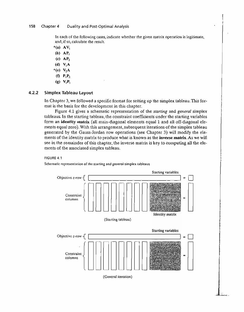
158 Chapter 4 Duality and Post-Optimal Analysis
In each of the following cases, indicate whether the given matrix operation is legitimate,and, if so, calcula te the resul t.
*(a) AVt
(b) API
(c) APz(d) VIA
*(e) V2A
(f) PlPZ
(g) VIPl
4.2.2 Simplex Tableau Layout
In Chapter 3, we followed a specific format for setting up the simplex tableau. This format is the basis for the development in this chapter.
Figure 4.1 gives a schematic representation of the starting and general simplextableaus. In the starting tableau, the constraint coefficients under the starting variablesform an identity matrix (all main-diagonal elements equal 1 and all off-diagonal elements equal zero). With this arrangement, subsequent iterations of the simplex tableaugenerated by the Gauss-Jordan row operations (see Chapter 3) will modify the elements of the identity matrix to produce what is known as the inverse matrix. As we willsee in the remainder of this chapter, the inverse matrix is key to computing all the elements of the associated simplex tableau.
FIGURE 4.1
Schematic representation of the starting and general simplex tableaus
Starting variables
Objective z-row { I I'--.------------ D
Constraintcolumns
Identity matrix
(Starting tableau)
Starting variables
Objective z-row {IL I 0
Constraintcolumns
(General iteration)
.~'":.••~-'<..- .•.
4.2 Primal-Dual Relationships 159
PROBLEM SET 4.2B
1. Consider the optimal tableau of Example 3.3-1.*(a) Identify the optimal inverse matrix.(b) Show that the right-hand side equals the inverse multiplied by the original right
hand side vector of the original constraints.2. Repeat Problem 1 for the last tableau of Example 3.4-1.
4.2.3 Optimal Dual Solution
TIle primal and dual solutions are so closely related that the optimal solution of eitherproblem directly yields (with little additional computation) the optimal solution to theother. Thus, in an LP model in which the number of variables is considerably smallerthan the number of constraints, computational savings may be realized by solving thedual, from which the primal solution is determined automatically. This result followsbecause the amount of simplex computation depends largely (though not totally) onthe number of constraints (see Problem 2, Set 4.2c).
This section provides two methods for determining the dual values. Note that thedual of the dual is itself the primal, which means that the dual solution can also be usedto yield the optimal primal solution automatically.
Method 1.
(0' I f) (Optimal primal z-coefficient of starting variable Xi)phmal va ue 0 = +
dual variable YiOriginal objective coefficient of Xi
Method 2.
. (ROW vector of )° timal values . . " .( f d
p . bl ) = ongmal obJectlve coefficIentso ual vana es . .
of optimal primal baSIC variables
x (Opti.mal primal)Inverse
The elements of the row vector must appear in the same order in which the basic variables are listed in the Basic column of the simplex tableau.
Example 4.2-1
Consider the following LP:
Maximize z = 5Xl + 12x2 + 4x)
subject to
Xl + 2X2 + x3 :s 10
2Xl - X2 + 3X3 = 8
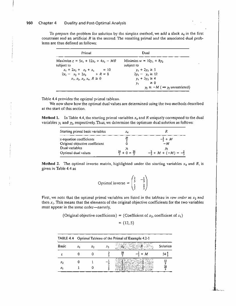
160 Chapter 4 Duality and Post-Optimal Analysis
To prepare the problem for solution by the simplex method, we add a slack X4 in the firstconstraint and an artificial R in the second. The resulting primal and the associated dual problems are thus defined as follows:
Primal
Maximize z = 5x, + 12x2 + 4x] - MRsubject to
XI + 2x2 + X3 + X4 = 102x1 - x2 + ~xJ + R = 8
Xl> X2. X], X4, R :;::: 0
Dual
Minimize w = lOy! + 8Y2subject to
YI + 2Y2 :;::: 52YI - Y2 ~ 12
YI + 3>'2 :;::: 4YI :;::: 0
Y2 :;::: - M ( =Y2 unrestricted)
Table 4.4 provides the optimal primal tableau.We now show how the optimal dual values are determined using the two methods described
at the start of this section.
Method 1. In Table 4.4. the starting primal variables X4 and R uniquely correspond to the dualvariables Yl and Yz, respectively. Thus, we determine the optimum dual solution as follows:
Starting primal basic variables
z-equation coefficientsOriginal objective coefficientDual variablesOptimal dual values
29"5oY,
~+o-~5 ~ 5
R
-~ + M5-M
Y2-~ + M + (-M) = -~
Method 2. The optimal inverse matrix, highlighted under the starting variables X4 and R, isgiven in Table 4.4 as
Optimal inve~ =(l -I)First, we note that the optimal primal variables are listed in the tableau in row order as X2 andthen XI' This means that the elements of the original objective coefficients for the two variablesmust appear in the same order-namely,
(Original objective coefficients) = (Coefficient of X2, coefficient of XI)
= (12,5)
TABLE 4.4 Optimal Tableau of the Primal of Example 4.2-1
Basic
z
X2
x,
o
o1
o
1
o
35"
~ -~ + M5 5
Solution
12"526"5
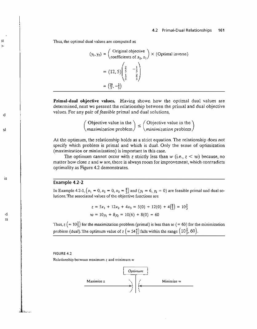
4.2 Primal-Dual Relationships 161
st)-
Thus, the optimal dual values are computed as
(Original objective ) ..
(y\, Y2) = ff· . f X (Optimal mverse)coe lClents 0 X2, Xl
:d
Primal-dual objective values. Having shown how the optimal dual values aredetermined, next we present the relationship between the primal and dual objectivevalues. For any pair ofjeasibLe primal and dual solutions,
3.1 (Objective value in the) ( Objective value in the)maximization problem ::s minimization problem
At the optimum, the relationship holds as a strict equation. The relationship does notspecify which problem is primal and which is dual. Only the sense of optimization(maximization or minimization) is important in this case.
The optimum cannot occur with z strictly less than w (i.e., z < w) because, nomatter how close z and ware, there is always room for improvement, which contradictsoptimality as Figure 4.2 demonstrates.
isExample 4.2-2
In Example 4.2-1, (Xl = 0, X2 = 0, X3 = ~) and (Yl = 6, Y2 = 0) are feasible primal and dual solutions.TIle associated values of the objective functions are
z = 5Xl + 12x2 + 4X3 = 5(0) + 12(0) + 4(~) = lO~
w = lOYI + 81'2 = 10(6) + 8(0) = 60
Thus, z (= 10~) for the maximization problem (primal) is less than w (= 60) for the minimization
problem (dual). The optimum value of z (= 54~) falls within the range (10~, 60).
FIGURE 4.2
Relationship between maximum z and minimum w
MinimizewMaximizezL~:tUn[:~J
----------l.~} ;..of4t-----------I ', I, ,
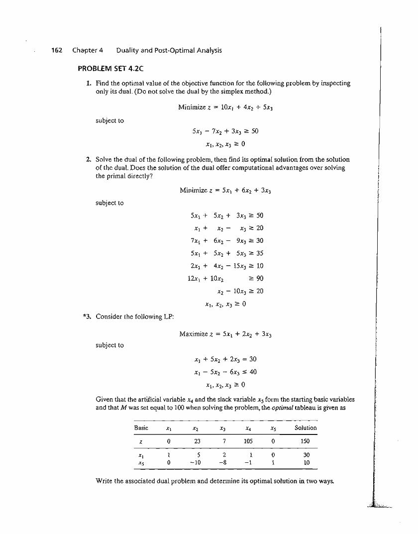
162 Chapter 4 Duality and Post-Optimal Analysis
PROBLEM SET 4.2C
1. Find the optimal value of the objective function for the following problem by inspectingonly its dual. (Do not solve the dual by the simplex method.)
Minimize z = lOx) + 4X2 + 5X3
subject to
2. Solve the dual of the following problem, then find its optimal solution from the solutionof the dual. Does the solution of the dual offer computational advantages over solvingthe primal directly?
Minimize z = 5Xl + 6X2 + 3X3
subject to
5Xl + 5X2 + 3X3;Z: 50
Xl + X2 - x3;Z: 20
7Xl + 6x2 - 9X3 2: 30
5x) + 5X2 + 5X3;Z: 35
2Xl + 4X2 - 15x3 ;z: 10
12xl + 10x2 ~ 90
x2 - 10x3 ;;:: 20
*3. Consider the following LP:
Maximize z = 5Xl + 2X2 + 3X3
subject to
Xl + 5X2 + 2X3 = 30
Xl - 5X2 - 6X3 S; 40
Given that the artificial variable X4 and the slack variable X5 form the starting basic variablesand that M was set equal to 100 when solving the problem, the optimal tableau is given as
Basic
z o
1o
Xz
23
5-10
7
2-8
105
1-1
oo1
Solution
150
3010
I
Write the associated dual problem and determine its optimal solution in two ways.
.. ,j i.~·.·.. ·.. .' :_...
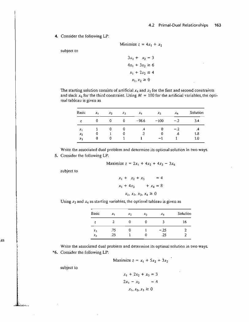
4.2 Primal-Dual Relationships 163
4. Consider the following LP:
Minimize z = 4x, + X2
subject to
3Xl + X2 = 3
4X1 + 3X2 ;::: 6
XI + 2X2 :0:; 4
The starting solution consists of artificial X4 and Xs for the first and second constraintsand slack X6 for the third constraint. Using M = 100 for the artificial variables, the optimal tableau is given as
Basic XI X2 X3 X4 Xs x6 Solution
z 0 0 0 -98.6 -100 -.2 3.4
XI 1 0 0 .4 0 -.2 .4Xl 0 1 0 .2 0 .6 1.8
x3 0 0 1 1 -1 1 1.0
Write the associated dual problem and determine its optimal solution in two ways.5. Consider the following LP:
Maximize z = 2xI + 4X2 + 4x) - 3X4
subject to
Using X) and X4 as starting variables, the optimal tableau is given as
Basic Xl
Z 2
XJ .75X2 .25
o
o1
o
1o
3
-.25.25
Solution
16
22
.es
It
.j tL.··.·: .' ~_...
Write the associated dual problem and determine its optimal solution in two ways.
*6. Consider the following LP:
Maximize z = XI + 5X2 + 3X3
subject to
XI + 2X2 + X3 = 3
2xI - X2 = 4
Xl, X2, X3 ;::: 0
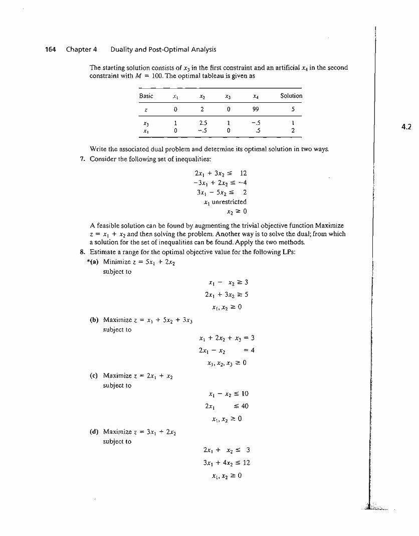
164 Chapter 4 Duality and Post-Optimal Analysis
The starting solution consists of x) in the first constraint and an artificial X4 in the secondconstraint with M = 100. The optimal tableau is given as
Basic Xl X2 X3 X4 Solution
z 0 2 0 99 5
.1:3 1 2.5 1 -.5 14.2x, 0 -.5 0 .5 2
Write the associated dual problem and determine its optimal solution in two ways.
7. Consider the following set of inequalities:
2xI + 3X2:::; 12-3Xl + 2x2 :::; -4
3Xl - 5x2:::; 2
Xl unrestricted
X2 ~ 0
A feasible solution can be found by augmenting the trivial objective function MaximizeZ = XI + X2 and then solving the problem. Another way is to solve the dual; from whicha solution for the set of inequalities can be found. Apply the two methods.
8. Estimate a range for the optimal objective value for the following LPs:
*(a) Minimize z = 5XI + 2X2
subject to
Xl - X2 ~ 3
2x} + 3X2 ~ 5
(b) Maximize z = Xl + 5X2 + 3x)
subject toXl + 2X2 + x3 = 3
2xI - X2 = 4
(c) Maximize z = 2xI + X2
subject toXI - X2 :$ 10
2Xl :$ 40
(d) Maximize z = 3xj + 2X2
subject to2xI + X2:::; 3
3x} + 4x2 :::; 12
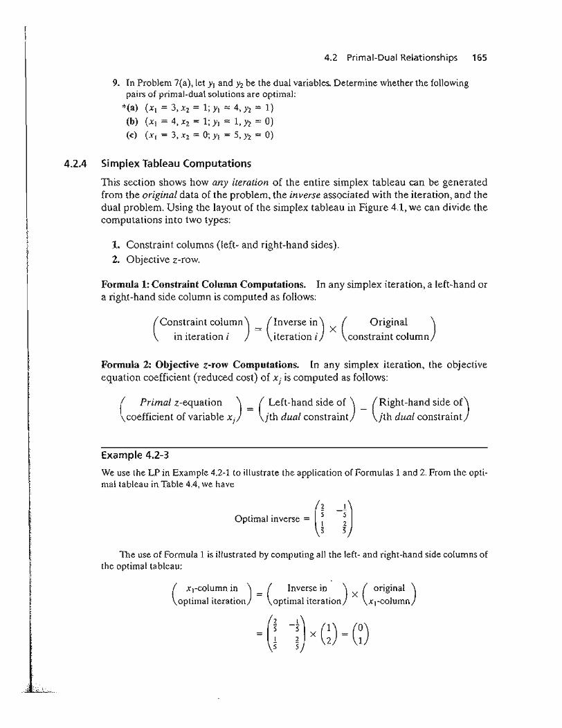
4.2 Primal-Dual Relationships 165
9. In Problem 7(a}, let Yl and Y2 be the dual variables. Determine whether the followingpairs of primal-dual solutions are optimal:
*(a) (Xl = 3,X2 = l;Yl = 4'Y2 = 1)
(b) (XI = 4, x2 = 1; YI = 1, Y2 = 0)(c) (XI = 3, X2 = 0; YI = 5, Y:z = 0)
4.2.4 Simplex Tableau Computations
This section shows how any iteration of the entire simplex tableau can be generatedfrom the original data of the problem, the inverse associated with the iteration, and thedual problem. Using the layout of the simplex tableau in Figure 4.1, we can divide thecomputations into two types:
1. Constraint columns (Ieft- and right-hand sides).
2. Objective z-row.
Formula 1: Constraint Column Computations. In any simplex iteration, a left-hand ora right-hand side column is computed as follows:
(co~st:aint ~ol~mn) = (~nver~e i~) X ( Original )III IteratiOn l IteratiOn 1 constraint column
Formula 2: Objective z-row Computations. In any simplex iteration, the objectiveequation coefficient (reduced cost) of xi is computed as follows:
(Primal z-equation ) ( Left-hand side of ) (Right-hand side Of)
coefficient of variable xi = jth dual constraint - jth dual constraint
Example 4.2-3
We use the LP in Example 4.2-1 to illustrate the application of Formulas 1 and 2. From the optimal tableau in Table 4.4, we have
(2 -5521)Optimal inverse = :
The use of Formula 1 is illustrated by computing all the left- and right-hand side columns ofthe optimal tableau:
(x]-column in) ( Inverse in ) (original)
optimal iteration = optimal iteration X XI-column
166 Chapter 4 Duality and Post-Optimal Analysis
In a similar manner, we compute the remaining constraint columns; namely,
(! . ) (ZXTCO umn In 5
optimal iteration := ~
(I . ) (2X3-CO umn 10 5
optimal iteration - !
( . ) (2x4-co!umn 10 :5optimal iteratio~ := ~
(R-column in ) (~
optimal iteration := ~
-I) X CD ~ G)
-I) X G) ~ (-:)
-I) X G) ~m-D X (~) ~ ( -I)
(Right-hand. Side) = (xz) = (~ -~) (10) = (¥)
column In Xl! ~ x 8 ~optimal iteration 5 5 5
Next, we demonstrate how the objective row computations are carried out using Formula 2.
TIle optimal values of the dual variables, (Yr. Yz) = (¥-, -~), were computed in Example 4.2-1
using two different methods. These values are used in Formula 2 to determine the associated zcoefficients; namely,
z-cofficient of Xl = Yl + 2yz - 5 = ¥- + 2 x -~ - 5 = 0
z-cofficient of X2 = 2Yl - yz - 12 := 2 x¥-- (-n - 12 = 0
z-cofficientofx3 = Yl + 3yz - 4 = ¥+ 3 x -~ - 4 ~
z-cofficient of X4 = Yl - 0 = ¥- 0 = ¥-z-cofficient of R = Y2 - (-M) = -~ - (-M) = -~ + M
Notice that Formula 1 and Formula 2 calculations can be applied at any iteration of eitherthe primal or the dual problems. All we need is the inverse associated with the (primal or dual)iteration and the original LP data.
PROBLEM SET 4.20
1. Generate the first simplex iteration of Example 4.2-1 (you may use TORA's Iterations=> M-method for convenience), then use Formulas 1 and 2 to verify all the elements ofthe resulting tableau.
2. Consider the following LP model:
Maximize z = 4x) + 14x2
subject to2x] + txz + X3 = 21
7x) + 2X2 + X4 = 21
xl> x2, x3' X4 ~ 0
4.2 Primal-Dual Relationships 167
Check the optimality and feasibility of each of the following basic solutions.
*(a) Basic variables = (X2, X4), Inverse = (_~ ~)7
(b) Basic variables = (X2' X3), Inverse = (~ j)2
7 2(c) Basic variables = (X2, xd, Inverse = (_~ -~)
45 45)
~)(d) Basic variables = (x), X4), Inverse = (_~2
3. Consider the following LP model:
Maximize z = 3x) + 2X2 + 5x3
subject to
2.
·1
= 30
+ X5 = 60
+ x6 = 20
c;-
Check the optimality and feasibility of the following basic solutions:
Basic variables ~ (x" XJ, x,), Inverse ~ G 1
D-2
(a) 12
0
1 1
-~)Basic v"iables ~ (X2, XJ, x,), Invme ~ ( i -8(b) _!
4
~r -1 12 2
I)
Basic variables ~ (X2, x" x,), Inverse ~ ( ~_1
D4
(c) )
2-2 1
*4. Consider the following LP model:
Minimize z = 2x) + X2
subject to
=3
=6
+ Xs = 3
",J"~I
II! 168 Chapter 4 Duality and Post-Optimal Analysis
Compute the entire simplex tableau associated with the following basic solution andcheck it for optimality and feasibility.
(3 _-15351 O~)Basic variables ~ (XI> X" x,), Inverse ~ -!
5. Consider the following LP model:
Maximize z = 5XI + 12x2 + 4x~
subject toXl + 2X2 + X3 + X4 == 10
2XI - X2 + 3X3 == 2
(a) Identify the best solution from among the following basic feasible solutions:
(1 --3il)(i) Basic variables = (X4. X3), Inverse = 0
(~ ---~~)(ii) Basic variables = (X2, Xl)' Inverse = i
(;! -77-21_)(iii) Basic variables = (X2, X3), Inverse = ~
(b) Is the solution obtained in (a) optimum for the LP model?
6. Consider the following LP model:
Maximize z = 5XI + 2X2 + 3X3
subject to
Xl + 5x2 + 2x3 :s bi
Xl - 5X2 - 6X3 :s b2
Xl> X2, X3 ~ 0
The following optimal tableau corresponds to specific values of b} and ~:
Basic Xl X2 X3 X4 Xs Solution
z 0 a 7 d e 150
Xl 1 b 2 1 0 30Xs 0 c -8 -1 1 10
Determine the following:(a) The right-hand-side values, bi and &2'
(b) The optimal dual solution,(c) The elements a, b, C, d, e.
. 1:..:=-::.......:... _...
4.;
4.3 Economic Interpretation of Duality 169
*7. TIle following is the optimal tableau for a maximization LP model with three (:s;) constraints and all nonnegative variables. The variables X3, X4, and Xs are the slacks associated with the three constraints. Determine the associated optimal objective value in twodifferent ways by using the primal and dual objective functions.
Basic XI X2 X3 X4 X, Solution
Z 0 0 0 3 2 ?
X3 0 0 1 1 -1 2X2 0 1 0 1 0 6XI 1 0 0 -1 1 2
8. Consider the following LP:
Maximize z = 2x] + 4x2 + 4xJ - 3X4
subject to
Xl + X2 + XJ = 4
x I + 4X2 + X4 = 8
Use the dual problem to show that the basic solution (Xl, X2) is not optimal.
9. Show that Method 1 in Section 4.2.3 for determining the optimal dual values is actuallybased on the Formula 2 in Section 4.2.4.
4.3 ECONOMIC INTERPRETATION OF DUALITY
The linear programming problem can be viewed as a resource allocation model inwhich the objective is to maximize revenue subject to the availability of limited resources. Looking at the problem from this standpoint, the associated dual problem offers interesting economic interpretations of the LP resource allocation model.
To formalize the discussion, we consider the following representation of the general primal and dual problems:
Primal
"Maximize z == Lqj
j~1
subject to"2. Qih :=:; bi , i '" 1, 2, ... , m
j=1
Xi 2: 0, j=l, 2, ... , n
Dual
111
Minimize w == LbiYi;=1
subject tom
2:aijYi 2= Cj' j == 1, 2, ... , ni=l
Yi 2: 0, i == 1, 2, ... , m
Viewed as a resource allocation model, the primal problem has n economic activitiesand m resources. The coefficient Cj in the primal represents the revenue per unit ofactivity j. Resource i, whose maximum availability is bi , is consumed at the rate aij unitsper unit of activity j.
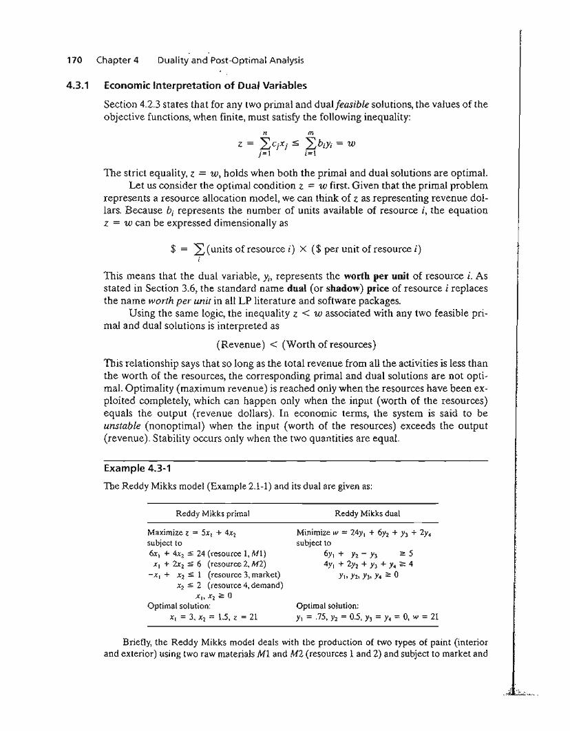
170 Chapter 4 Duality and Post-Optimal Analysis
4.3.1 Economic Interpretation of Dual Variables
Section 4.2.3 states that for any two primal and dual feasible solutions, the values of theobjective functions, when finite, must satisfy the following inequality:
n m
Z = 2:CjXj s; 2:biYi = Wj==l i==l
The strict equality, z = w, holds when both the primal and dual solutions are optimal.Let us consider the optimal condition z = 'W first. Given that the primal problem
represents a resource allocation model, we can think of z as representing revenue dollars. Because bi represents the number of units available of resource i, the equationz = w can be expressed dimensionally as
$ = 2: (units of resource i) X ($ per unit of resource i)i
This means that the dual variable, Yi> represents the worth per unit of resource i. Asstated in Section 3.6, the standard name dual (or shadow) price of resource i replacesthe name worth per unit in all LP literature and software packages.
Using the same logic, the inequality z < w associated with any two feasible primal and dual solutions is interpreted as
(Revenue) < (Worth of resources)
This relationship says that so long as the total revenue from all the activities is less thanthe worth of the resources, the corresponding primal and dual solutions are not optimal. Optimality (maximum revenue) is reached only when the resources have been exploited completely, which can happen only when the input (worth of the resources)equals the output (revenue dollars). In economic terms, the system is said to beunstable (nonoptimal) when the input (worth of the resources) exceeds the output(revenue). Stability occurs only when the two quantities are equal.
Example 4.3-1
The Reddy Mikks model (Example 2.1-1) and its dual are given as:
Reddy Mikks primal
Maximize z = 5xI + 4X2
subject to6x1 + 4X2 :S 24 (resource 1, Ml)
XI + 2x2 :S 6 (resource 2, M2)- X I + x2 :S 1 (resource 3, market)
X2 :S 2 (resource 4, demand)x"x22:0
Optimal solution:XI = 3, X2 = 1.5, z = 21
Reddy Mikks dual
Minimize IV = 24YI + 6yz + Y3 + 2Y4subject to
6Yl + Y2 - Y3 2: 54YI + 2Y2 + Y3 + Y4 2: 4
Yh Y2, Y3. Y4 2: 0
Optimal solution:YI = .75, Y2 = 0.5, Y3 = Y4 = 0, w = 21
Briefly, the Reddy Mikks model deals with the production of two types of paint (interiorand exterior) using two raw materials Ml and M2 (resources 1 and 2) and subject to market and
1
1
ss
l-
4.3 Economic Interpretation of Duality 171
demand limits represented by the third and fourth constraints. The model determines theamounts (in tons/day) of interior and exterior paints that maximize the daily revenue (expressedin thousands of dollars).
The optimal dual solution shows that the dual price (worth per unit) of raw material Ml (resource 1) is Yl = .75 (or $750 per ton), and that of raw material M2 (resource 2) is Y2 = .5 (or$500 per ton). These results hold true for specific feasibility ranges as we showed in Section 3.6.For resources 3 and 4, representing the market and demand limits, the dual prices are both zero,which indicates that their associated resources are abundant. Hence, their worth per unit is zero.
PROBLEM SET 4.3A
1. In Example 4.3-1, compute the change in the optimal revenue in each of the followingcases (use TORA output to obtain the feasibility ranges):
(a) The constraint for raw material M1 (resource 1) is 6Xl + 4X2 $ 22.
(b) The constraint for raw material M2 (resource 2) is Xl + 2X2 $ 4.5.
(c) The market condition represented by resource 4 is X2 $ 10.
*2. NWAC Electronics manufactures four types of simple cables for a defense contractor.Each cable must go through four sequential operations: splicing, soldering, sleeving, andinspection. The following table gives the pertinent data of the situation.
Minutes per unit
Cable Splicing Soldering Sleeving IllSpeclion Unit revenue ($)ni- SC320 10.5 2004 3.2 5.0 9.40
(- SC325 9.3 24.6 2.5 5.0 10.80
;) SC340 11.6 17.7 3.6 5.0 8.75S070 8.2 26.5 5.5 5.0 7.80
IeIt Daily capacity (minutes) 4800.0 9600.0 4700.0 4500.0
.ornd
-< - :~~,~",. ~
The contractor guarantees a minimum production level of 100 units for each of the fourcables.
(a) Formulate the problem as a linear programming model, and determine the optimumproduction schedule.
(b) Based on the dual prices, do you recommend making increases in the daily capacitiesof any of the four operations? Explain.
(c) Does the minimum production requirements for the four cables represent an advantage or a disadvantage for NWAC Electronics? Provide an explanation based on thedual prices.
(d) Can the present unit contribution to revenue as specified by the dual price be guaranteed if we increase the capacity of soldering by 1O%?
3. BagCo produces leather jackets and handbags. A jacket requires 8 m2 of leather, and ahandbag only 2 m2• The labor requirements for the two products are 12 and 5 hours, respectively. The current weekly supplies of leather and labor are limited to 1200 m2 and1850 hours. The company sells the jackets and handbags at $350 and $120, respectively.The objective is to determine the production schedule that maximizes the net revenue.BagCo is considering an expansion of production. What is the maximum purchase pricetile company should pay for additional leather? For additional labor?
ij'I0'"
JI
.!j 172 Chapter 4 Duality and Post-Optimal Analysis
4.3.2 Economic Interpretation of Dual Constraints
The dual constraints can be interpreted by using Formula 2 in Section 4.2.4, whichstates that at any primal iteration,
Ob" ff' . f (Left-hand side Of) (Right-hand side Of)~ectlve coe IClent 0 x· == -
J dual constraint j dual constraint jm
= L aijYi - Cj;=1
We use dimensional analysis once again to interpret this equation. The revenue perunit, Cj, of activity j is in dollars per unit. Hence, for consistency, the quantity L:1aijYimust also be in dollars per unit. Next, because Cj represents revenue, the quantity2:;~laijYi' which appears in the equation with an opposite sign, must represent cost.Thus we have
m 111 (usage of resource i ) (cost per unit)$ cost = LaijYi = 2: X
i=l i=1 per unit of activity j of resource i
The conclusion here is that the dual variable Yi represents the imputed cost per unit ofresource i, and we can think of the quantity L;~1aijYi as the imputed cost of all the resources needed to produce one unit of activity j.
In Section 3.6, we referred to the quantity CL;:1aijYi - Cj) as the reduced costof activity j. The maximization optimality condition of the simplex method says thatan increase in the level of an unused (nonbasic) activity j can improve revenue only ifits reduced cost is negative. In terms of the preceding interpretation, this conditionstates that
(
Imputed cost Of) R .evenue er umtresources used by < ( f .~ . )
. '" 0 activIty]one umt of actIvIty]
The maximization optimality condition thus says that it is economically advantageous to increase an activity to a positive level if its unit revenue exceeds its unit imputed cost.
We will use the TOYCO model of Section 3.6 to demonstrate the computation.The details of the model are restated here for convenience.
Example 4.3-2
TOYCO assembles three types of toys: trains, trucks, and cars using three operations. Availableassembly times for the three operations are 430,460, and 420 minutes per day, respectively, andthe revenues per toy train, truck, and car are $3, $2, and $5, respectively. The assembly times pertrain for the three operations are 1,3, and 1 minutes, respectively. The corresponding times pertruck and per car are (2,0,4) and (1,2,0) minutes (a zero time indicates that the operation isnot used).
.,' -:.~ .....':.;:..:...-'~.. .
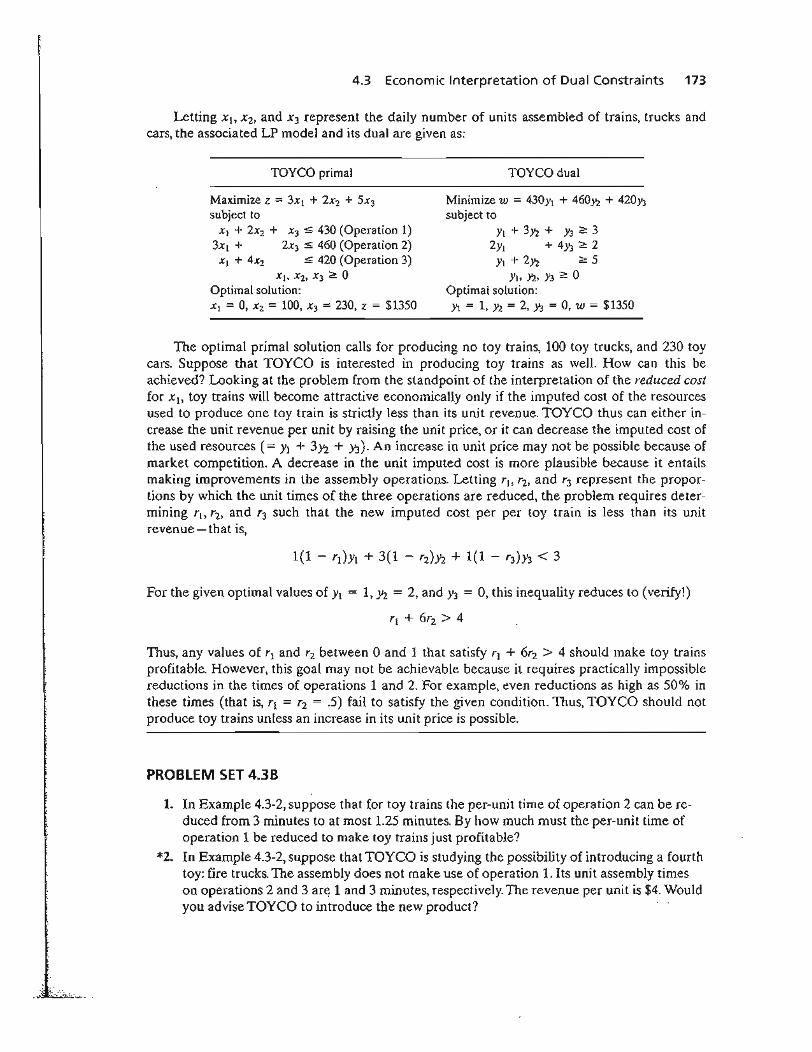
4.3 Economic Interpretation of Dual Constraints 173
Letting Xl> X2, and X3 represent the daily number of units assembled of trains, trucks andcars, the associated LP model and its dual are given as:
TOYCO primal
Maximize z == 3Xl + 2X2 + 5X3subject to
Xl + 2X2 + x3::; 430 (Operation 1)3xI + 2X3 ::; 460 (Operation 2)
Xl + 4X2 ::; 420 (Operation 3)xI> x2, x3 ~ °
Optimal solution:XI = 0, X2 = 100, x3 = 230, z = $1350
TOYCO dual
Minimize w == 430Yl + 460Yl + 420Y3subject to
Yl + 3Y2 + Y3 ~ 32Yl + 4Y3 '2: 2
YI + 2Yl ~ 5Y" }2, Y3 ~ 0
Optimal solution:Yl == 1, Y2 == 2, .Y3 == 0, W = $1350
1.ed:r *2.:ris
.,~ -,;,.".......~:.:.:.-- .....
The optimal primal solution calls for producing no toy trains, 100 toy trucks, and 230 toycars. Suppose that TOYCO is interested in producing toy trains as well. How can this beachieved? Looking at the problem from the standpoint of the interpretation of the reduced costfor xl> toy trains will become attractive economically only if the imputed cost of the resourcesused to produce one toy train is strictly less than its unit revenue. TOYCO thus can either increase the unit revenue per unit by raising the unit price, or it can decrease the imputed cost ofthe used resources (= YI + 3Y2 + Y3). An increase in unit price may not be possible because ofmarket competition. A decrease in the unit imputed cost is more plausible because it entailsmaking improvements in the assembly operations. Letting rl: r2, and r3 represent the proportions by which the unit times of the three operations are reduced, the problem requires determining rl> '2, and r3 such that the new imputed cost per per toy train is less than its unitrevenue-that is,
For the given optimal values of Yl = 1, Y2 = 2, and Y3 = 0, this inequality reduces to (verify!)
r. + 6"2 > 4
Thus, any values of 'I and 1"2 between 0 and 1 that satisfy 1"1 + 6r2 > 4 should make toy trainsprofitable. However, this goal may not be achievable because it requires practically impossiblereductions in the times of operations 1 and 2. For example, even reductions as high as 50% inthese times (that is, rl = r2 = .5) fail to satisfy the given condition. Thus, TOYCO should notproduce toy trains unless an increase in its unit price is possible.
PROBLEM SET 4.3B
In Example 4.3-2, suppose that for toy trains the per-unit time of operation 2 can be reduced from 3 minutes to at most 1.25 minutes. By how much must the per-unit time ofoperation 1 be reduced to make toy trains just profitable?
In Example 4.3-2, suppose that TOYCO is studying the possibility of introducing a fourthtoy: fire trucks. The assembly does not make use of operation 1. Its unit assembly timeson operations 2 and 3 are 1 and 3 minutes, respectively. The revenue per unit is $4. Wouldyou advise TOYCO to introduce the new product?
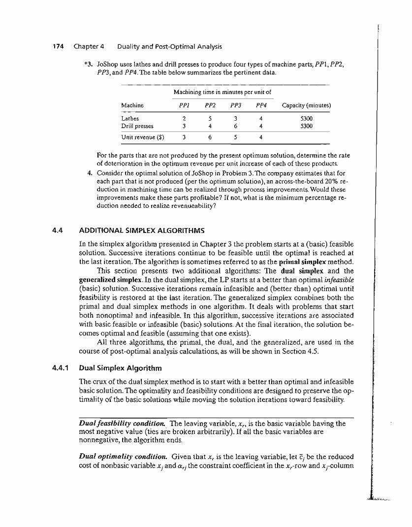
174 Chapter 4 Duality and Post-Optimal Analysis
*3. JoShop uses lathes and drill presses to produce four types of machine parts, PPl, PPl,PP3, and PP4. The table below summarizes the pertinent data.
Machining time in minutes per unit of
Machine PPI PP2 PP3 PP4 Capacity (minutes)
Lathes 2 5 3 4 5300Drill presses 3 4 6 4 5300
Unit revenue ($) 3 6 5 4
For the parts that are not produced by the present optimum solution, determine the rateof deterioration in the optimum revenue per unit increase of each of these products.
4. Consider the optimal solution of JoShop in Problem 3. The company estimates that foreach part that is not produced (per the optimum solution), an across-the-board 20% re
. duction in machining time can be realized through process improvements. Would theseimprovements make these parts profitable? If not, what is the minimum percentage reduction needed to realize revenueability?
4.4 ADDITIONAL SIMPLEX ALGORITHMS
In the simplex algorithm presented in Chapter 3 the problem starts at a (basic) feasiblesolution. Successive iterations continue to be feasible until the optimal is reached atthe last iteration. The algorithm is sometimes referred to as the primal simplex method.
This section presents two additional algorithms: The dual simplex and thegeneralized simplex. In the dual simplex, the LP starts at a better than optimal infeasible(basic) solution. Successive iterations remain infeasible and (better than) optimal untilfeasibility is restored at the last iteration. The generalized simplex combines both theprimal and dual simplex methods in one algorithm. It deals with problems that startboth nonoptimal and infeasible. In this algorithm, successive iterations are associatedwith basic feasible or infeasible (basic) solutions. At the final iteration, the solution becomes optimal and feasible (assuming that one exists).
All three algorithms, the primal, the dual, and the generalized, are used in thecourse of post-optimal analysis calculations, as will be shown in Section 4.5.
4.4.1 Dual Simplex Algorithm
The crux of the dual simplex method is to start with a better than optimal and infeasiblebasic solution. The optimality and feasibility conditions are designed to preserve the optimality of the basic solutions while moving the solution iterations toward feasibility.
Dual feasibility condition. The leaving variable, X n is the basic variable having themost negative value (ties are broken arbitrarily). If all the basic variables arenonnegative, the algorithm ends.
Dual optimality condition. Given that X r is the leaving variable, let c; be the reducedcost of nonbasic variable x; and Urj the constraint coefficient in the xr-row and xrcolumn
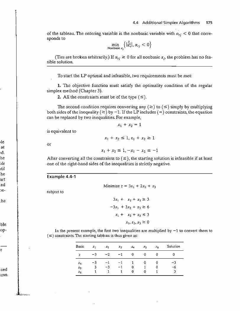
lieat.d.heJleItilheart:edJe-
:he
bleop-
.cedImn
4.4 Additionat Simplex Algorithms 175
of the tableau. The entering variable is the nonbasic variable with a'i < 0 that corresponds to
(Ties are broken arbitrarily.) If a.,j ::> 0 for all nonbasic Xj, the problem has no feasible solution.
To start the LP optimal and infeasible, two requirements must be met:
1. The objective function must satisfy the optimality condition of the regularsimplex method (Chapter 3).
2. All the constraints must be of the type (:::;).
The second condition requires converting any (~) to (:::::;) simply by multiplyingboth sides of the inequality (~) by -1. If the LP includes (=) constraints, the equationcan be replaced by two inequalities. For example,
Xl + X2 = 1
is equivalent to
or
After converting all the constraints to (:::::;), the starting solution is infeasible if at leastone of the right-hand sides of the inequalities is strictly negative.
Example 4.4-1
Minimize z = 3x} + 2X2 + X3
subject to
Xl + X2 + X3 S 3
xl. X2, X3 2 0
In the present example, the first two inequalities are multiplied by -1 to convert them to( :5) constraints. The starting tableau is thus given as:
Basic XI X2 x3 X4 Xs X6 Solution
z -3 -2 -1 0 0 0 0
X4 -3 -1 -1 1 0 0 -'-3
Xs 3 -3 -1 0 1 0 -6X6 1 1 1 0 0 1 3
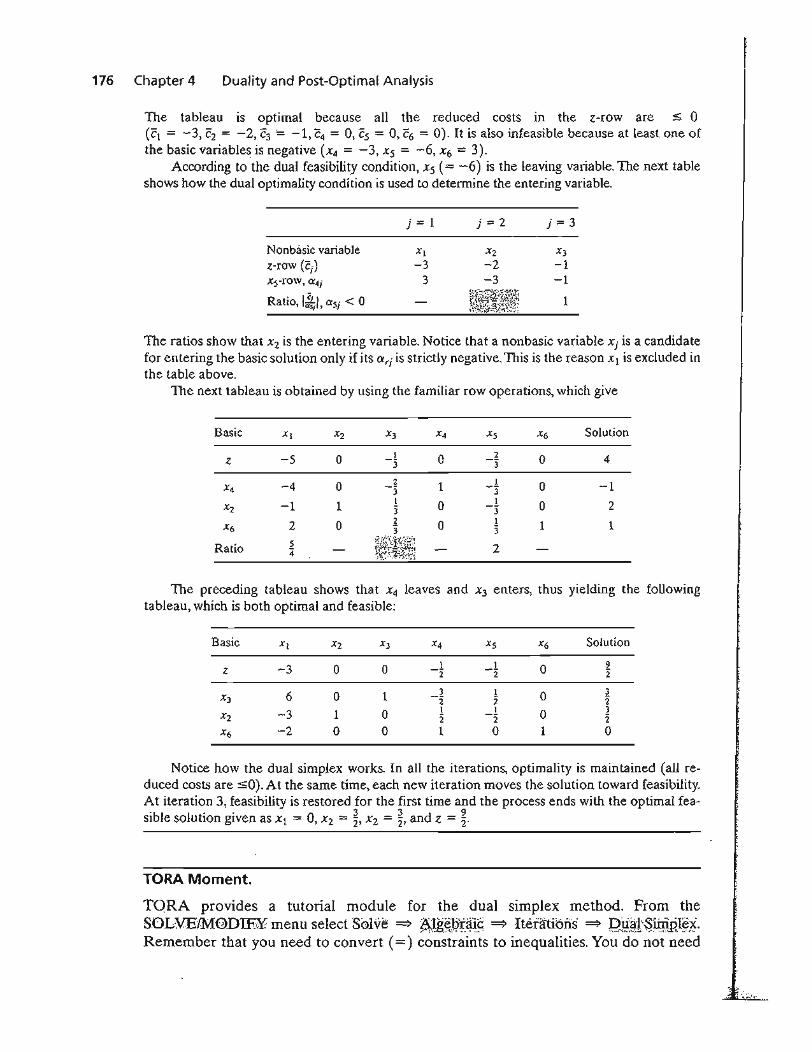
176 Chapter 4 Duality and Post-Optimal Analysis
The tableau is optimal because all the reduced costs in the z-row are s °(Cl = -3, (;2 = -2, C3= -1, C4 = 0, (;5 = 0, C6 = 0). It is also infeasible because at least one ofthe basic variables is negative (X4 = -3, X5 = -6, X6 = 3).
According to the dual feasibility condition, Xs (= -6) is the leaving variable. The next tableshows how the dual optimality condition is used to determine the entering variable.
Nonbasic variablez-row (Cj)X5-row, fX4j
Ratio, I~I, CiSj < 0
j = 1
Xl
-33
j=2
XJ
-1-1
1
The ratios show that Xl is the entering variable. Notice that a nonbasic variable Xj is a candidatefor entering the basic solution only if its Clrj is strictly negative. This is the reason Xl is excluded inthe table above.
The next tableau is obtained by using the familiar row operations, which give
Basic Xl X2 X3 X4 Xs X6 Solution
-5 0 I 0 2 0 4z -3 -3
-4 0 2 1 _1 0 -1X4 -3 3
-1 1 I 0 1 0 2X2 3 -32 0 2 0 1 1 1X6 3 3
Ratio 2 ~~~~~ 24
The preceding tableau shows that X4 leaves and X3 enters, thus yielding the followingtableau, which is both optimal and feasible:
Basic Xl X2 ):3 X4 X5 X6 Solution
-3 0 0 I 1 0 9z -2 -2 2
6 0 1 3 1 0 3xJ -2 2" 2"
-3 1 0 1 1 0 3X2 2" -2 2"X6 -2 0 0 1 0 1 0
Notice how the dual simplex works. In all the iterations, optimality is maintained (all reduced costs are ~o).At the same time, each new iteration moves the solution toward feasibility.At iteration 3, feasibility is restored for the first time and the process ends with the optimal fea-'bl I" 0 3 3 d 9Sl e so utron gIVen as Xl = , Xl = 2' X2 = 2' an z = 2'
TORA Moment.
TQRA provides a tutorial module for the dual simplex method. From theSOLVEIMOD1F¥ menu select SblVe ~ A:~g~Jit~~ ~ IteratiOiiS ~ ;Qg~t§@.Rli#.?'·
Remember that you need to convert (=) constraints to inequalities. You do not need
" ; ":'to ~".;.
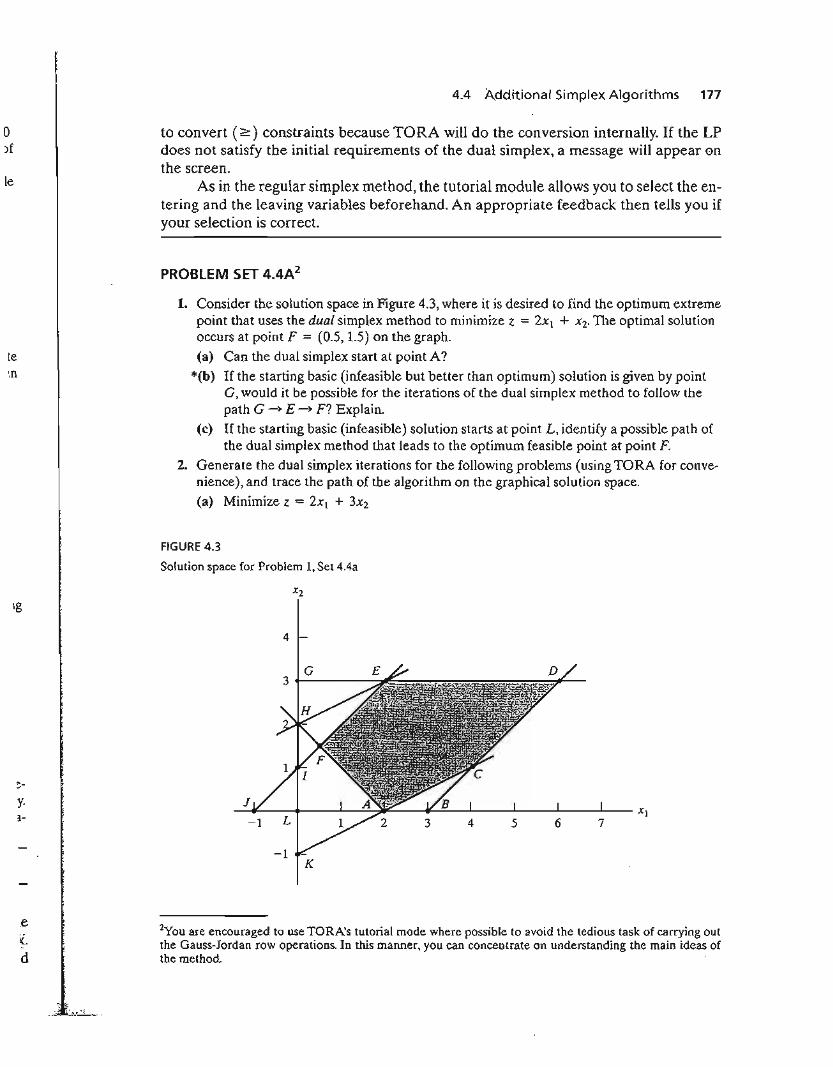
le
tein
y.1-
.eIed
4.4 A~ditional Simplex Algorithms 177
to convert (2:) constraints because TORA will do the conversion internally. If the LPdoes not satisfy the initial requirements of the dual simplex, a message will appear onthe screen.
As in the regular simplex method, the tutorial module allows you to select the entering and the leaving variables beforehand. An appropriate feedback then tells you ifyour selection is correct.
PROBLEM SET 4.4A2
1. Consider the solution space in Figure 4.3, where it is desired to find the optimum extremepoint that uses the dual simplex method to minimize z = 2xt + X2' TIle optimal solutionoccurs at point F = (0.5,1.5) on the graph.
(a) Can the dual simplex start at point A?
*(b) If the starting basic (infeasible but better than optimum) solution is given by pointG, would it be possible for the iterations of the dual simplex method to follow thepath G~ E~ F? Explain.
(c) If the starting basic (infeasible) solution starts at point L, identify a possible path ofthe dual simplex method that leads to the optimum feasible point at point F.
2. Generate the dual simplex iterations for the following problems (usingTORA for convenience), and trace the path of the algorithm on the graphical solution space.
(a) Minimize z = 2xt + 3X2
FIGURE 4.3
Solution space for Problem 1, Set 4.4a
4
2you are encouraged to use TORA's tutorial mode where possible to avoid the tedious task of carrying outthe Gauss-Jordan row operations. In this manner, you can concentrate on understanding the main ideas ofthe method.
178 Chapter 4 Duality and Post-Optimal Analysis
subject to2Xl + 2X2 :$ 30
Xl + 2X2 =::: 10
x" X2 =::: 0
(b) Minimize z == 5Xl + 6X2
subject to
Xl + X2 2: 2
4xl + X2 2: 4
Xl, X2 2: 0
(c) Minimize z == 4Xl + 2X2
subject to
Xl + X2 == 1
3Xl - X2 =::: 2
Xl> X2 =::: 0
(d) Minimize z == 2XI + 3X2
subject to
3. Dual Simplex with Artificial Constraints. Consider the following problem:
Maximize z = 2XI - X2 + X3
subject to
2XI + 3X2 - 5x3 =::: 4
- Xl + 9X2 - x3 =::: 3
4XI + 6X2 + 3X3 :$ 8
The starting basic solution consisting of surplus variables X4 and Xs and slack variable X6
is infeasible because X4 == -4 and Xs = -3. However, the dual simplex is not applicabledirectly, because Xl and x3 do not satisfy the maximization optimality condition. Showthat by adding the artificial constraint Xl + X3 :$ M (where M is sufficiently large not toeliminate any feasible points in the original solution space), and then using the new constraint as a pivot row, the selection of Xl as the entering variable (because it has the mostnegative objective coefficient) will render an all-optimal objective row. Next, carry outthe regular dual simplex method on the modified problem.
'';':;:'.~-'-
o
st
4.4 Additional Simplex Algorithms 179
4. Using the artificial constraint procedure introduced in Problem 3, solve the followingproblems by the dual simplex method. In each case, indicate whether the resulting solution is feasible, infeasible, or unbounded.
(a) Maximize z = 2X3
subject to
(b) Maximize z := Xl - 3x2
subject to
*(c) Minimize z = -xl + X2
subject to
Xl - 4X2 ;::: 5
Xl - 3X2 :5 1
2xI - 5X2 ;::: 1
(d) Maximize z = 2X3
subject to
5. Solve the following LP in three different ways (useTORA for convenience). Whichmethod appears to be the most efficient computationally?
subject to
5XI + 6X2 - 3X3 + 4X4 ;::: 12
X2 - 5X3 - 6X4 ;::: 10
2XI + 5X2 + x3 + x4;::: 8
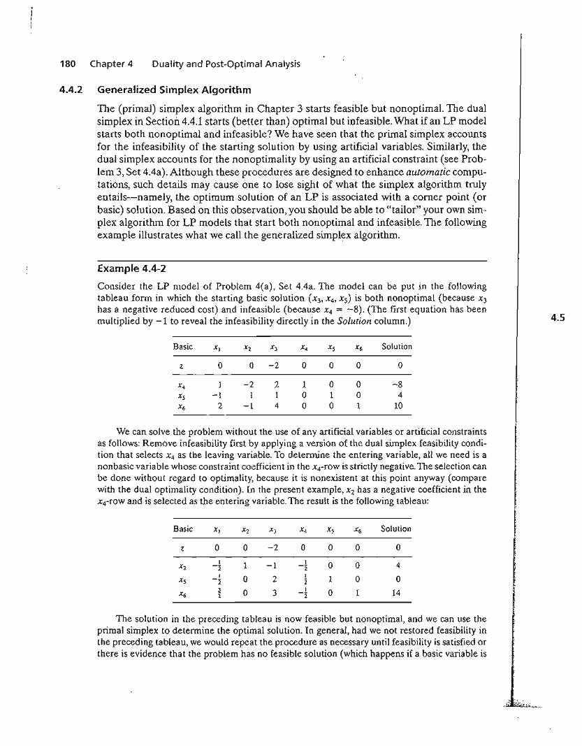
180 Chapter 4 Duality and Post-Optimal Analysis
4.4.2 Generalized Simplex Algorithm
The (primal) simplex algorithm in Chapter 3 starts feasible but nonoptimal. The dualsimplex in Section 4.4.1 starts (better than) optimal but infeasible. What if an LP modelstarts both nonoptimal and infeasible? We have seen that the primal simplex accountsfor the infeasibility of the starting solution by using artificial variables. Similarly, thedual simplex accounts for the nonoptimality by using an artificial constraint (see Problem 3, Set 4.4a).Although these procedures are designed to enhance automatic computations, such details may cause one to lose sight of what the simplex algorithm trulyentails-namely, the optimum solution of an LP is associated with a comer point (orbasic) solution. Based on this observation, you should be able to "tailor" your own simplex algorithm for LP models that start both nonoptimal and infeasible. The followingexample illustrates what we call the generalized simplex algorithm.
Example 4.4-2
Consider the LP model of Problem 4(a), Set 4.4a. The model can be put in the followingtableau form in which the starting basic solution (X3, X4, xs) is both nonoptimal (because X3
has a negative reduced cost) and infeasible (because X4 = -8). (The first equation has beenmultiplied by -1 to reveal the infeasibility directly in the Solution column.)
Basic Xl X2 X3 X4 Xs X6 Solution
z 0 0 -2 0 0 0 0
X4 1 -2 2 1 0 0 -8Xs -1 1 1 0 1 0 4
X6 2 -1 4 0 0 1 10
We can solve the problem without the use of any artificial variables or artificial constraintsas follows: Remove infeasibility first by applying a version of the dual simplex feasibility condition that selects X4 as the leaving variable. To determine the entering variable, all we need is anonbasic variable whose constraint coefficient in the X4-row is strictly negative. The selection canbe done without regard to optimality, because it is nonexistent at this point anyway (comparewith the dual optimality condition). In the present example, X2 has a negative coefficient in thex4-rowand is selected as the entering variable. The result is the following tableau:
Basic Xl X2 x) X4 Xs x6 Solution
z 0 0 -2 0 0 0 0
1 1 -1 1 0 0 4X2 -2 -2I 0 2 I 1 0 0Xs -2 2
x63 0 3 I 0 1 142 -2
fTIle solution in the preceding tableau is now feasible but nonoptimal, and we can use the
primal simplex to determine the optimal solution. In general, had we not restored feasibility inthe preceding tableau, we would repeat the procedure as necessary until feasibility is satisfied orthere is evidence that the problem has no feasible solution (which happens if a basic variable is
4.5
4.5 Post-Optimal Analysis 181
negative and all its constraint coefficients are nonnegative). Once feasibility is established, thenext step is to pay attention to optimality by applying the proper optimality condition of the primal simplex method.
Remarks. The essence of Example 4.4-2 is that the simplex method is not rigid. The literatureabounds with variations of the simplex method (e.g., the primal-dual method, the symmetricalmethod, the criss-cross method, and the multiplex method) that give the impression that eachprocedure is different, when, in effect, they all seek a corner point solution, with a slant towardautomated computations and, perhaps, computational efficiency.
PROBLEM SET 4.4B
1. The LP model of Problem 4(c), Set 4.4a, has no feasible solution. Show how this condition is detected by the generalized simplex procedure.
2. TIle LP model of Problem 4(d), Set 4.4a, has no bounded solution. Show how this condition is detected by the generalized sirnplex procedure.
4.5 POST-OPTIMAL ANALYSIS
In Section 3.6, we dealt with the sensitivity of the optimum solution by determining theranges for the different parameters that would keep the optimum basic solution unchanged. In this section, we deal with making changes in the parameters of the modeland finding the new optimum solution. Take, for example, a case in the poultry industrywhere an LP model is commonly used to determine the optimal feed mix per broiler(see Example 2.2-2). The weekly consumption per broiler varies from .26 lb (120grams) for a one-week-old bird to 2.11b (950 grams) for an eight-week-old bird. Additionally, the cost of the ingredients in the mix may change periodically. These changesrequire periodic recalculation of the optimum solution. Post-optimal analysis determines the new solution in an efficient way. The new computations are rooted in the useduality and the primal-dual relationships given in Section 4.2.
The following table lists the cases that can arise in post-optimal analysis and theactions needed to obtain the new solution (assuming one exists):
Condition after parameters change
Current solution remains optimal and feasible.Current solution becomes infeasible.Current solution becomes nonoptimal.Current solution becomes both nonoptimaland infeasible.
Recommended action
No further action is necessary.Use dual simplex to recover feasibility.Use primal simplex to recover optimality.Use the generalized simplex method to obtain newsolution.
The first three cases are investigated in this section. The fourth case, being a combination of cases 2 and 3, is treated in Problem 6, Set 4.5a.
The TOyeO model of Example 4.3-2 will be used to explain the different procedures. Recall that the TOyeD model deals with the assembly of three types of. toys:trains, trucks, and cars. Three operations are involved in the assembly. We wish to
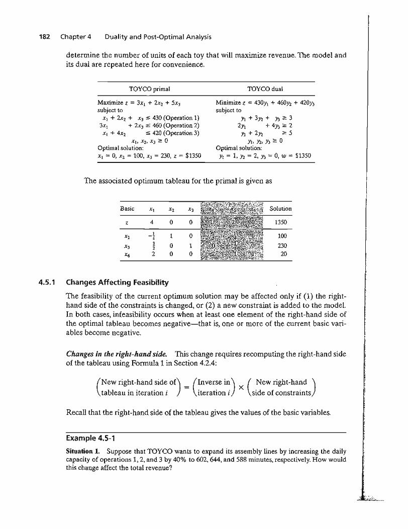
182 Chapter 4 Duality and Post-Optimal Analysis
determine the number of units of each toy that will maximize revenue. The model andits dual are repeated here for convenience.
TOYCO primal TOYCOdual
Maximize z == 3xI + 2X2 + 5X3subject to
Xl + 2X2 + x3 :S 430 (Operation 1)3Xl + 2X3 :S 460 (Operation 2)
Xl + 4X2 :S 420 (Operation 3)Xh X2, X3 2: 0
Optimal solution:XI == 0, X2 == 100, X3 = 230, Z = $1350
Minimize z == 430YI + 460Y2 + 420Y3subject to
Yt + 3Y2 + Y3;::: 32YI + 4Y3 ;::: 2
YI + 2Y2 2: 5Yh Y2, Y3 2: 0
Optimal solution:Yl "" 1, Y2 = 2, Y3 == 0, W == $1350
The associated optimum tableau for the primal is given as
Basic Xl X2 X3 Solution
z 4 0 0 1350
X2_! 1 0 1004
X3 ~ 0 1 2302
x6 2 0 0 20
4.5.1 Changes Affecting Feasibility
The feasibility of the current optimum solution may be affected only if (1) the righthand side of the constraints is changed, or (2) a new constraint is added to the model.In both cases, infeasibility occurs when at least one element of the right-hand side ofthe optimal tableau becomes negative-that is, one or more of the current basic variables become negative.
Changes in the right-hand side. This change requires recomputing the right-hand sideof the tableau using Formula 1 in Section 4.2.4:
(New right-hand side Of) (Inverse in) (New right-hand )tableau in iteration i = iteration i X side of constraints
Recall that the right-hand side of the tableau gives the values of the basic variables.
Example 4.5-1
Situation 1. Suppose that TOYCO wants to expand its assembly lines by increasing the dailycapacity of operations 1,2, and 3 by 40% to 602, 644, and 588 minutes, respectively. How wouldthis change affect the total revenue?
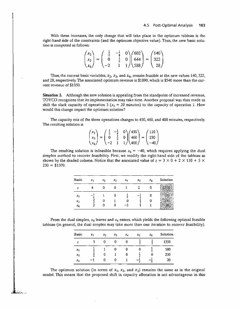
4.5 Post-Optimal Analysis 183
With these increases, the only change that will take place in the optimum tableau is theright-hand side of the constraints (and the optimum objective value). Thus, the new basic solution is computed as follows:
-! ~)(~~) = (~~~)1 1 588 28
Thus, the current basic variables, x2, x3, and x6, remain feasible at the new values 140,322,and 28, respectively. The associated optimum revenue is $1890, which is $540 more than the current revenue of $1350.
Situation 2. Although the new solution is appealing from the standpoint of increased revenue,TOYCO recognizes that its implementation may take time. Another proposal was thus made toshift the slack capacity of operation 3 (X6 = 20 minutes) to the capacity of operation 1. Howwould this change impact the optimum solution?
The capacity mix of the three operations changes to 450,460, and 400 minutes, respectively.The resulting solution is
The resulting solution is infeasible because X6 = -40, which requires applying the dualsimplex method to recover feasibility. First, we modify the right-hand side of the tableau asshown by the shaded column. Notice that the associated value of z = 3 X 0 + 2 X 110 + 5 X
230 = $1370.
Basic
z 4 o
1
oo
o
o1o
1
17:o
-2
2 o
oo1
Solution
~~~..~.i,~.'.!..!~,.~~~;. .. J.
From the dual simplex, X6 leaves and X4 enters, which yields the following optimal feasibletableau (in general, the dual simplex may take more than one iteration to recover feasibility).
Basic Xl Xz X3 X4 Xs X6 Solution
Z 5 0 0 0 5 1 13507: 7:1 1 0 0 0 ! 100Xl 4" 43 0 1 0 I 0 230x3 7: 2
X4 -1 0 0 1 _! _1 20 .I 2
The optimum solution (in terms of xl> x2, and x3) remains the same as in the originalmodel. This means that the proposed shift in capacity allocation is not advantageous }Pr this-
184 Chapter 4 Duality and Post-Optimal Analysis
f
case because all it does is shift the surplus capacity in operation 3 to a surplus capacity in operation 1. TIle conclusion is that operation 2 is the bottleneck and it may be advantageous toshift the surplus to operation 2 instead (see Problem 1, Set 4.5a). The selection of operation 2over operation 1 is also reinforced by the fact that the dual price for operation 2 ($2/mi11) ishigher than that for operation 2 (= $l/min).
PROBLEM SET 4.5A
1. In the TOYCO model listed at the start of Section 4.5, would it be more advantageous toassign the 20-minute excess capacity of operation 3 to operation 2 instead of operation I?
2. Suppose that TOYCO wants to change the capacities of the three operations according tothe following cases:
(
460)(a) 500
400(
500)(b) 400
600(c) (~~)
200(
450)(d) 700
350
Use post-optimal analysis to determine the optimum solution in each case.
3. Consider the Reddy Mikks model of Example 2.1-1. Its optimal tableau is given in Example 3.3-1. If the daily availabilities of raw materials Ml and M2 are increased to 28 and 8tons, respectively, use post-optimal analysis to determine the new optimal solution.
*4. The Ozark Farm has 20,000 broilers that are fed for 8 weeks before being marketed. Theweekly feed per broiler varies according to the following schedule:
Week
Iblbroiler
1
.26
2
.48
3
.75
4
1.00
5
1.30
6
1.60
7
1.90
8
2.10
For the broiler to reach a desired weight gain in 8 weeks, the feedstuffs must satisfy specific nutritional needs. Although a typical list of feedstuffs is large, for simplicity we willlimit the model to three items only: limestone, corn, and soybean meaL The nutritionalneeds will also be limited to three types: calcium, protein, and fiber. The following tablesummarizes the nutritive content of the selected ingredients together with the cost data.
Content (Ib) per Ib of
Ingredient Calcium Protein Fiber $ per lb
Limestone .380 .00 .00 .12Corn .001 .09 .02 .45Soybean meal .002 .50 .08 1.60
The feed mix must contain
(a) At least .8% but not more than 1.2% calcium
(b) At least 22% protein
(c) At most 5% crude fiberSolve the LP for week 1 and then use post-optimal analysis to develop an optimal
. schedule for the remaining 7 weeks.
";'~~'';''...
4.5 Post-Optimal Analysis 185
5. Show that the 100% feasibility rule in Problem 12, Set 3.6c (Chapter 3) is based on thecondition
(?Ptimum)(Origi~alright-hand) ;=: 0mverse side vector
6. Post-optimal Analysis for Cases Affecting Both Optimality and Feasibility. Supposethat you are given the following simultaneous changes in the Reddy Mikks model:The revenue per ton of exterior and interior paints are $1000 and $4000, respectively,and the maximum daily availabilities of raw materials, M1 and M2, are 28 and 8 lons,respectively.
(a) Show that the proposed changes will render the current optimal solution bothnonoptimal and infeasible.
(b) Use the generalized simplex algorithm (Section 4.4.2) to determine the new optimalfeasible solution.
Addition of New Constraints. The addition of a new constraint to an existing modelcan lead to one of two cases.
1. The new constraint is redundant, meaning that it is satisfied by the current optimum solution, and hence can be dropped from the model altogether.
2. The current solution violates the new constraint, in which case the dual simplexmethod is used to restore feasibility.
Notice that the addition of a new constraint can never improve the current optimum objective value.
Example 4.5-3
Situation 1. Suppose that TOYCO is changing the design of its toys, and that the change will require the addition of a fourth operation in the assembly lines. The daily capacity of the new operation is 500 minutes and the times per unit for the three products on this operation are 3, 1, and1 minutes, respectively. Study the effect of the new operation on the optimum solution.
The constraint for operation 4 is
3Xl + X2 + X3 5 500
This constraint is redundant because it is satisfied by the current optimum solution Xl ::;: 0,X2 ::;: 100, and X3 = 230. Hence, the current optimum solution remains unchanged.
Situation 2. Suppose, instead, that TOYCO unit times on the fourth operation are changed to3, 3, and 1 minutes, respectively. All the remaining data of the model remain the same. Will theoptimum solution change?
The constraint for operation 4 is
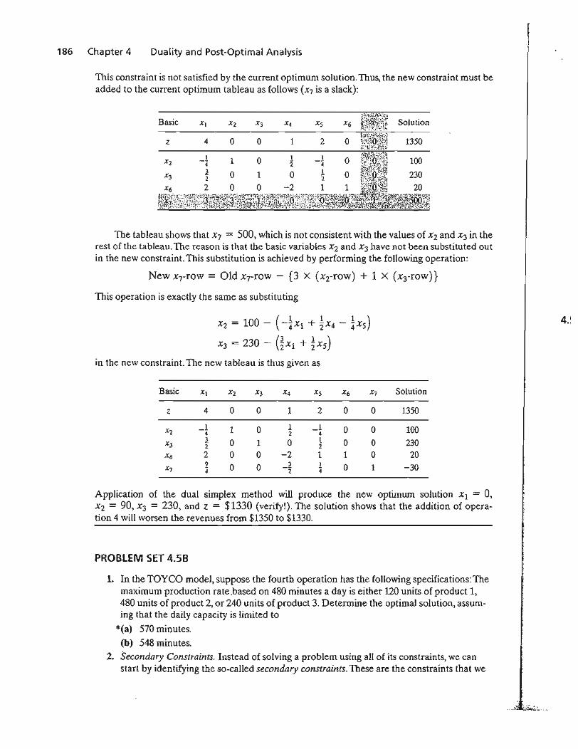
186 Chapter 4 Duality and Post-Optimal Analysis
This constraint is not satisfied by the current optimum solution.Thus, the new constraint must beadded to the current optimum tableau as follows (X7 is a slack):
Basic Xl X2 X3 X4 X5 X6
Z 4 0 0 1 2 0
X2I 1 0 1 1 0-4 '2 -43 0 1 0 1 0X3 2 2
X6 2 0 0 -2 1 1
Solution
1350
The tableau shows that X7 = 500, which is not consistent with the values of Xz and x3 in therest of the tableau. The reason is that the basic variables X2 and x3 have not been substituted outin the new constraint. TIlis substitution is achieved by performing the following operation:
New X7-fOW = Old X7-row - {3 X (xTrow) + 1 X (X3-roW)}
This operation is exactly the same as substituting
Xz = 100- (1 1 1)-4X1 + 2" X4 - 4XS
X3 = 230 - (~Xl+!X5)
in the new constraint. The new tableau is thus given as
Basic Xl X2 X3 X4 X5 X6 .'(7 Solution
z 4 0 0 1 2 0 0 1350
_1 1 0 .1 1 a 0 100x2 4 2 -43 0 1 0 1 0 0 230X3 2 2
X6 2 0 0 -2 1 1 0 209 0 0 3 1 0 1 -30X7 :1 -2 4
Application of the dual simplex method will produce the new optimum solution Xl = 0,Xz = 90, X3 == 230, and z = $1330 (verify!). The solution shows that the addition of operation 4 will worsen the revenues from $1350 to $1330.
PROBLEM SET 4.58
1. In the TOYCO model, suppose the fourth operation has the following specifications: Themaximum production rate.based on 480 minutes a day is either 120 units of product 1,480 units of product 2, or 240 units of product 3. Determine the optimal solution, assuming that the daily capacity is limited to
*(a) 570 minutes.
(b) 548 minutes.2. Secondary Constraints. Instead of solving a problem using all of its constraints, we can
start by identifying the so-called secondary constraints. These are the constraints that we
4.~
... ;;. ' ..~.:... -:';...:.
4.5 Post-Optimal Analysis 187
suspect are least restrictive in terms of the optimum solution. The model is solved usingthe remaining (primary) constraints. We may then add the secondary constraints one at atime. A secondary constraint is discarded if it satisfies the available optimum. The processis repeated until all the secondary constraints are accounted for.
Apply the proposed procedure to the following LP:
Maximize z = 5Xl + 6X2 + 3X2
subject to
7Xl + 6X2 - 9X3 :$ 30
5Xl + 5X2 + 5X3 :$ 35
12xl + 6X2 :$ 90
X2 - 9X3 :$ 20
4.5.2 Changes Affecting Optimality
This section considers two particular situations that could affect the optimality of thecurrent solution:
1. Changes in the original objective coefficients.2. Addition of a new economic activity (variable) to the model.
Changes in the Objective Function Coefficients. These changes affect only the optimalityof the solution. Such changes thus require recomputing the z-row coefficients (reducedcosts) according to the following procedure:
1. Compute the dual values using Method 2 in Section 4.2.3.2. Use the new dual values in Formula 2, Section 4.2.4, to determine the new re
duced costs (z-row coefficients).
Two cases will result:
1. New z-row satisfies the optimality condition. The solution remains unchanged(the optimum objective value may change, however).
2. The optimality condition is not satisfied. Apply the (primal) simplex method torecover optimality.
Example 4.5-4
Situation 1. In the TOYCO model, suppose that the company has a new pricing policy to meetthe competition. The unit revenues under the new policy are $2, $3, and $4 for train, truck, andcar toys, respectively. How is the optimal solution affected?
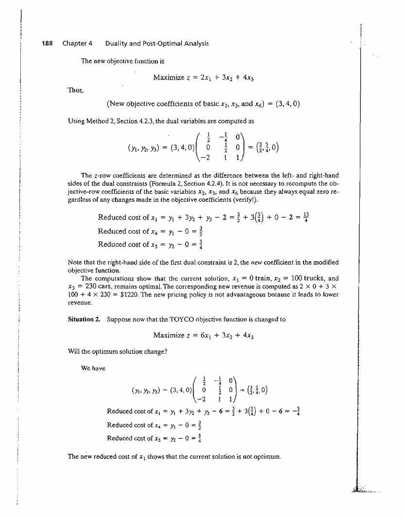
188 Chapter 4 Duality and Post-Optimal Analysis
The new objective function is
Maximize z = 2XI + 3X2 + 4X3
Thus,
(New objective coefficients of basic X2, X3, and X6) = (3,4,0)
Using Method 2, Section 4.2.3, the dual variables are computed as
The z-row coefficients are determined as the difference between the left- and right-handsides of the dual constraints (Fonnula 2, Section 4.2.4). It is not necessary to recompute the objective-row coefficients of the basic variables X2, x3, and x6 because they always equal zero regardless of any changes made in the objective coefficients (verify!).
Reduced cost of Xl = YI + 3Y2 + Y3 - 2 = ~ + 3(~) + 0- 2 = ~
Reduced cost of X4 = Yl - 0 = ~
Reduced cost of Xs = Y2 - 0 = ~
Note that the right-hand side of the first dual constraint is 2, the new coefficient in the modifiedobjective function.
The computations show that the current solution, Xl == 0 train, X2 = 100 trucks, andx3 = 230 cars, remains optimal. The corresponding new revenue is computed as 2 x 0 + 3 x100 + 4 x 230 = $1220. The new pricing policy is not advantageous because it leads to lowerrevenue.
Situation 2. Suppose now that the TOYCO objective function is changed to
Maximize z = 6XI + 3X2 + 4x)
Will the optimum solution change?
We have
(Yh)/2, Y3) = (3, 4, 0)( ~ -1 ~) = (~,~, 0)-2 1 1
Reduced cost of Xl = Yl + 3Y2 + Y3 - 6 = ~ + 3(~) + 0 - 6 = -~
Reduced cost of X4 = Yl - 0 = ~
Reduced cost of Xs = Y2 - 0 = ~
The new reduced cost of xl shows that the current solution is not optimum.
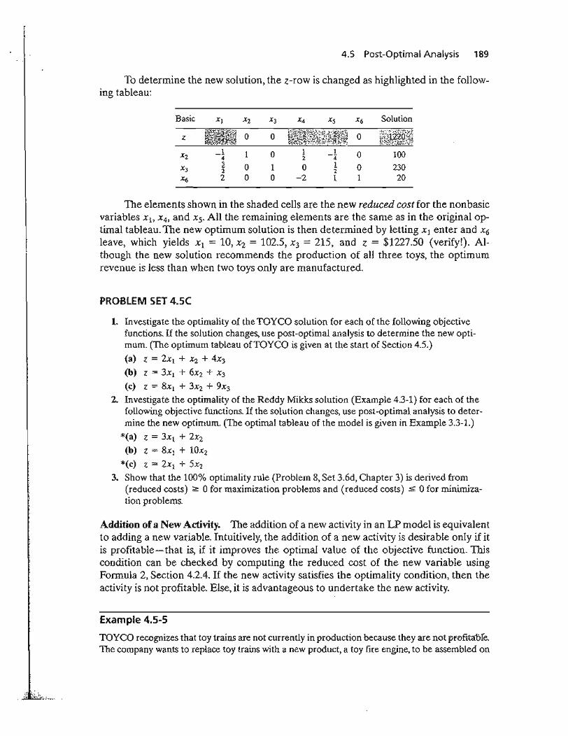
4.5 Post-Optimal Analysis 189
To determine the new solution, the z-row is changed as highlighted in the following tableau:
Basic Xl X2 X3 x'4 Xs X6 Solution
z 0 0 ~~i~~~~~~g~~¥¥~ 0 ~0~~~~~}
1 0 I 1 0 100X2 -4 2 -43 0 1 0 ! 0 230X3 2 2
X6 2 0 0 -2 1 1 20
The elements shown in the shaded cells are the new reduced cost for the nonbasicvariables Xl> X4, and Xs. All the remaining elements are the same as in the original optimal tableau. The new optimum solution is then determined by letting Xl enter and X6
leave, which yields Xl = 10, X2 = 102.5, X3 = 215, and z = $1227.50 (verify!). Although the new solution recommends the production of all three toys, the optimumrevenue is less than when two toys only are manufactured.
PROBLEM SET 4.5C
L Investigate the optimality of the TOYCO solution for each of the following objectivefunctions. If the solution changes, use post-optimal analysis to determine the new optimum. (The optimum tableau of TOYCO is given at the start of Section 4.5.)
(a) Z = 2x} + X2 + 4X3
(b) Z = 3x} + 6X2 + x3
(c) Z = 8x} + 3X2 + 9X3
2. Investigate the optimality of the Reddy Mikks solution (Example 4.3-1) for each of thefollowing objective functions. If the solution changes, use post-optimal analysis to determine the new optimum. (The optimal tableau of the model is given in Example 3.3-1.)
*(a) z = 3x} + 2X2
(b) z = 8x} + 10x2*(c) Z = 2xI + 5X2
3. Show that the 100% optimality rule (Problem 8, Set 3.6d, Chapter 3) is derived from(reduced costs) ~ 0 for maximization problems and (reduced costs) :::; 0 for minimization problems.
Addition ofa New Activity. The addition of a new activity in an LP model is equivalentto adding a new variable. Intuitively, the addition of a new activity is desirable only if itis profitable-that is, if it improves the optimal value of the objective function. Thiscondition can be checked by computing the reduced cost of the new variable usingFormula 2, Section 4.2.4. If the new activity satisfies the optimality condition, then theactivity is not profitable. Else, it is advantageous to undertake the new activity.
Example 4.5-5
TOYCO recognizes that toy trains are not currently in production because they are not prefitabre.The company wants to replace toy trains with a new product, a toy fire engine, to be assembled on
190 Chapter 4 Duality and Post-Optimal Analysis
the existing facilities. TOYCO estimates the revenue per toy fire engine to be $4 and the assemblytimes per unit to be 1 minute on each of operations 1 and 2, and 2 minutes on operation 3. Howwould this change impact the solution?
Let x7 represent the new fire engine product. Given that (Yl> Y2, Y3) = (1,2,0) are theoptimal dual values, we get
Reduced cost of X7 = lYl + lY2 + 2Y3 - 4 = 1 X 1 + 1 X 2 + 2 X 0 - 4 = -1
The result shows that it is profitable to include X7 in the optimal basic solution. To obtain thenew optimum, we first compute its column constraint using Formula 1, Section 4.2.4, as
(
1 17: -4
xrconstraint colum = 0 !-2 1
Thus, the current simplex tableau must be modified as follows
Basic Xl X2 X3 X4 Xs X6 Solution
z 4 0 0 1 2 0 1350
I 1 0 1 1 0 100X2 -4 2 -43 0 1 0 ! 0 230X3 2 2
-'=6 2 0 0 -2 1 1 20
The new optimum is determined by letting X7 enter the basic solution, in which case x6 mustleave. The new solution is Xl = 0, x2 = 0, x3 = 125, X7 = 210, and z = $1465 (verify!),which improves the revenues by $115.
PROBLEM SET 4.50
*1. In the original TOYCO model, toy trains are not part of the optimal product mix. Thecompany recognizes that market competition will not allow raising the unit price of thetoy. Instead, the company wants to concentrate on improving the assembly operation itself. This entails reducing the assembly time per unit in each of the three operations by aspecified percentage, p%. Determine the value of p that will make toy trains just profitable. (The optimum tableau of the TOYCO model is given at the start of Section 4.5.)
2. In the TOYCO model, suppose that the company can reduce the unit times on operations1,2, and 3 for toy trains from the current levels of 1,3, and 1 minutes to .5,1, and .5 minutes, respectively. The revenue per unit remains unchanged at $3. Determine the new optimum solution.
3. In the TOYCO model, suppose that a new toy (fire engine) requires 3, 2, 4 minutes, respectively, on operations 1,2, and 3. Determine the optimal solution when the revenueper unit is given by
*(a) $5.
(b) $10.
_,f ;.~~-.:...• _.
lSt
I),
a
inS
l-
p-
:..,t:~-.:...•..
References 191
4. In the Reddy Mikks model, the company is considering the production of a cheaperbrand of exterior paint whose input requirements per ton include .75 ton of each of rawmaterials Ml and M2. Market conditions still dictate that the excess of interior paint overthe production of both types of exterior paint be limited to 1 ton daily. The revenue perton of the new exterior paint is $3500. Determine the new optimal solution. (The model isexplained in Example 4.5-1, and its optimum tableau is given in Example 3.3-1.)
REFERENCES
Bradley, S., A. Hax, and T. Magnanti, Applied Mathematical Programming, Addison-Wesley,Reading, MA, 1977.
Bazaraa, M., 1. Jarvis, and H. Sherali, Linear Programming and Network Flows, 2nd ed., Wiley,New York, 1990.
Diwckar, 0., Introduction to Applied Optimization, Kluwer Academic Publishers, Boston, 2003.
Nering, E., and A. Tucker, Linear Programming and Related Problems, Academic Press, Boston,1992.
Vanderbei, R., Linear Programming: Foundation and Optimization,2nd ed., Kluwer AcademicPublishers, Boston MA, 2001.
CHAPTER 5
Transportation Modeland Its Variants
Chapter Guide. The transportation model is a special class of linear programs thatdeals with shipping a commodity from sources (e.g., factories) to destinations (e.g.,warehouses). The objective is to determine the shipping schedule that minimizes thetotal shipping cost while satisfying supply and demand limits. The application of thetransportation model can be extended to other areas of operation, including inventorycontrol, employment scheduling, and personnel assignment.
As you study the material in this chapter, keep in mind that the steps of the transportation algorithm are precisely those of the simplex method. Another point is thatthe transportation algorithm was developed in the early days of OR to enhance handcomputations. Now, with the tremendous power of the computer, such shortcuts maynot be warranted and, indeed, are never used in commercial codes in the strict mannerpresented in this chapter. Nevertheless, the presentation shows that the special transportation tableau is useful in modeling a class of problems in a concise manner (as opposed to the familiar LP model with explicit objective function and constraints). Inparticular, the transportation tableau format simplifies the solution of the problem byExcel Solver. The representation also provides interesting ideas about how the basictheory of linear programming is exploited to produce shortcuts in computations.
You will find TORA's tutorial module helpful in understanding the details of thetransportation algorithm. The module allows you to make the decisions regarding thelogic of the computations with immediate feedback.
This chapter includes a summary of 1 real-life application, 12 solved examples, 1Solver model, 4 AMPL models, 46 end-of-section problems, and 5 cases. The cases are inAppendix E on the CD.The AMPLlExcei/SolverrrORA programs are in folder chSFiles.
Real-life Application-Scheduling Appointments at Australian Trade Events
The Australian Tourist Commission (ATC) organizes trade events around the world toprovide a forum for Australian sellers to meet international buyers of tourism products, including accommodation, tours, and transport. During these events, sellers are
193
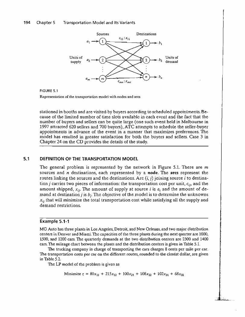
194 Chapter 5
FIGURE 5.1
Transportation Model and Its Variants
Sources
Units ofsupply
Destinations
Units ofb2 demand
btl
Representation of the transportation model with nodes and arcs
stationed in booths and are visited by buyers according to scheduled appointments. Because of the limited number of time slots available in each event and the fact that thenumber of buyers and sellers can be quite large (one such event held in Melbourne in1997 attracted 620 sellers and 700 buyers), ATC attempts to schedule the seller-buyerappointments in advance of the event in a manner that maximizes preferences. Themodel has resulted in greater satisfaction for both the buyers and sellers. Case 3 inChapter 24 on the CD provides the details of the study.
5.1 DEFINITION OF THE TRANSPORTATION MODEL
The general problem is represented by the network in Figure 5.1. There are msources and n destinations, each represented by a node. The arcs represent theroutes linking the sources and the destinations. Arc (i, j) joining source i to destination j carries two pieces of information: the transportation cost per unit, Cij, and theamount shipped, Xij' The amount of supply at source i is ai and the amount of demand at destinationj is bj • The objective ofthe model is to determine the unknownsXij that will minimize the total transportation cost while satisfying all the supply anddemand restrictions.
Example 5.1-1
MG Auto has three plants in Los Angeles, Detroit, and New Orleans, and two major distributioncenters in Denver and Miami. The capacities of the three plants during the next quarter are 1000,1500, and 1200 cars. The quarterly demands at the two distribution centers are 2300 and 1400cars. The mileage chart between the plants and the distribution centers is given in Table 5.l.
The trucking company in charge of transporting the cars charges 8 cents per mile per car.The transportation costs per car on the different routes, rounded to the closest dollar, are given f
. in Table 5.2.The LP model of the problem is given as
Minimize z = 80xu + 215x12 + lOOX21 + l08x22 + l02x31 + 68x32
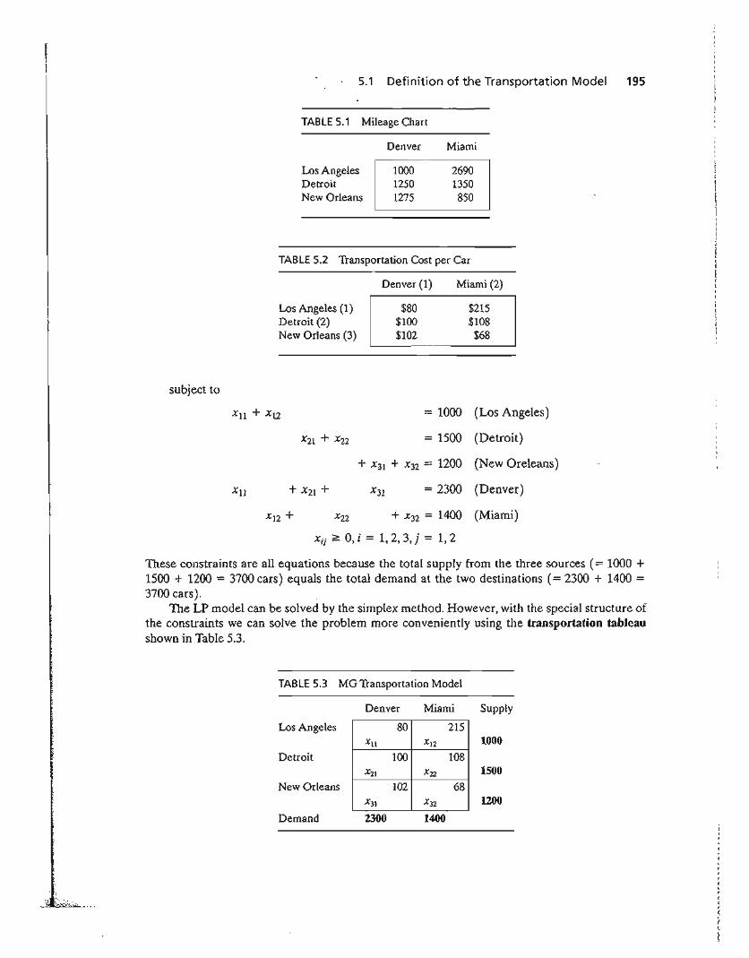
5.1 Definition of the Transportation Model 195
TABLE 5.1 Mileage Chart
Los AngelesDetroitNew Orleans
Denver
100012501275
Miami
26901350850
TABLE 5.2 Transportation Cost per Car
subject to
Los Angeles (1)Detroit (2)New Orleans (3)
Denver (1)
$80$100$102
Miami (2)
$215$108
$68
= 1000 (Los Angeles)
= 1500 (Detroit)
+ x31 + X32 = 1200 (New Oreleans)
+ x21 + = 2300 (Denver)
+ x32 = 1400 (Miami)
Xij ;;:;: 0, i = 1, 2, 3, j = 1, 2
These constraints are all equations because the total supply from the three sources (= 1000 +1500 + 1200 = 3700 cars) equals the total demand at the two destinations (= 2300 + 1400 =3700 cars).
The LP model can be solved by the simplex method. However, with the special structure ofthe constraints we can solve the problem more conveniently using the transportation tableaushown in Table 5.3.
TABLE 5.3 MG Transportation Model
Denver Miami Supply
Los Angeles
Detroit
New Orleans
80 215Xu X12
100 108X21 X22
102 68X31 X32
1000
1500
uooDemand 2300 1400
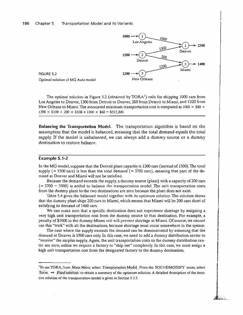
196 Cha pter 5 Transportation Model and Its Variants
FIGURE 5.2
Optimal solution of MG Auto model
1000
1500
uooNew Orleans
2300
1400
The optimal solution in Figure 5.2 (obtained by TORA1) calls for shipping 1000 cars from
Los Angeles to Denver, 1300 from Detroit to Denver, 200 from Detroit to Miami, and 1200 fromNew Orleans to Miami. The associated minimum transportation cost is computed as 1000 x $80 +1300 x $100 + 200 x $108 + 1200 x $68 = $313,200.
Balancing the Transportation Model. The transportation algorithm is based on theassumption that the model is balanced, meaning that the total demand equals the totalsupply. If the model is unbalanced, we can always add a dummy source or a dummydestination to restore balance.
Example 5.1-2
In the MG model, suppose that the Detroit plant capacity is 1300 cars (instead of 1500).The totalsupply (= 3500 cars) is less than the total demand (= 3700 cars), meaning that part of the demand at Denver and Miami will not be satisfied.
Because the demand exceeds the supply, a dummy source (plant) with a capacity of 200 cars(= 3700 - 3500) is added to balance the transportation model. The unit transportation costsfrom the dummy plant to the two destinations are zero because the plant does not exist.
Table 5.4 gives the balanced model together with its optimum solution. The solution showsthat the dummy plant ships 200 cars to Miami, which means that Miami will be 200 cars short ofsatisfying its demand of 1400 cars.
We can make sure that a specific destination does not experience shortage by assigning avery high unit transportation cost from the dummy source to that destination. For example, apenalty of $1000 in the dummy-Miami cell will prevent shortage at Miami. Of course, we cannotuse this "trick" with all the destinations, because shortage must occur somewhere in the system.
TIle case where the supply exceeds the demand can be demonstrated by assuming that thedemand at Denver is 1900 cars only. In this case, we need to add a dummy distribution center to"receive" the surplus supply. Again, the unit transportation costs to the dummy distribution center are zero, unless we require a factory to "ship out" completely. In this case, we must assign ahigh unit transportation cost from the designated factory to the dummy destination.
ITo use TORA, from ;Main Menu. select ·TranspOrtationMod'el. From theS~OLVE/rv10DIFYmenu, select
'Soive: ~'Fin~rSdlii'tiqi{ to obtain a su~mary '~i the ~pti~~~solution. A detailed description of the itera
tive solution of the transportation model is given in Section 5.3.3.
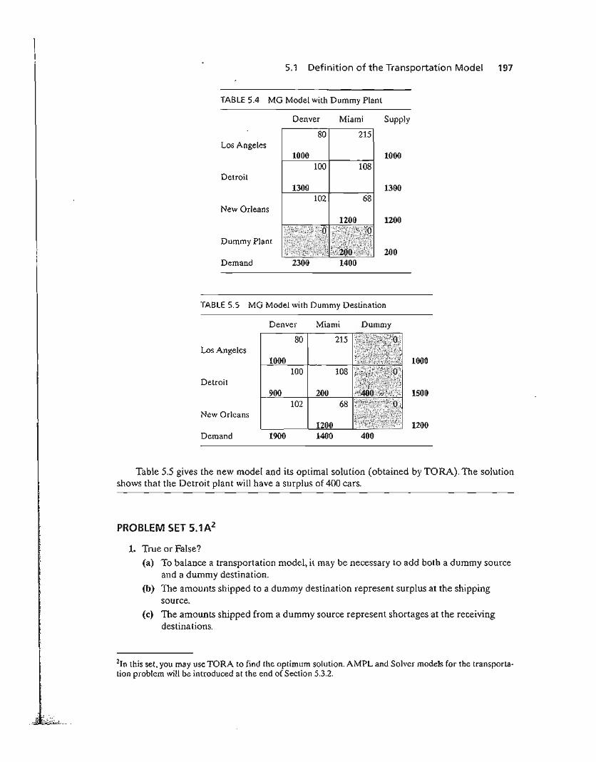
5.1 Definition of the Transportation Model 197
TABLE 5.4 MG Model with Dummy Plant
Denver Miami Supply
80 215Los Angeles
1000 1000100 108
Detroit1300 1300
102 68New Orleans
1200 1200
Demand 2300 1400200
TABLE 5.5 MG Model with Dummy Destination
PROBLEM SET 5.1A2
1500
1200
1000
Dummy
400
Denver Miami
80 215Los Angeles
1000100 108
Detroit900 200
102 68New Orleans
1200Demand 1900 1400
1. True or False?(a) To balance a transportation model, it may be necessary to add both a dummy source
and a dummy destination.
(b) The amounts shipped to a dummy destination represent surplus at the shippingsource.
(c) The amounts shipped from a dummy source represent shortages at the receivingdestinations.
2In this set, you may use TORA to find the optimum solution. AMPL and Solver models for the transportation problem will be introduced at the end of Section 5.3.2.
Table 5.5 gives the new model and its optimal solution (obtained by TORA). The solutionshows that the Detroit plant will have a surplus of 400 cars.
198 Chapter 5 Transportation Model and Its Variants
2. In each of the following cases, determine whether a dummy source or a dummy destination must be added to balance the model.
(a) Supply: al = 10, a2 = 5, a3 = 4, a4 = 6Demand: bi = 10, b2 = 5, b3 = 7, b4 = 9
(b) Supply: aJ = 30, Q2 = 44Demand: bJ = 25, bi = 30, b3 = 10
3. In Table 5.4 of Example 5.1-2, where a dummy plant is added, what does the solutionmean when the dummy plant "ships" 150 cars to Denver and 50 cars to Miami?
*4. In Table 5.5 of Example 5.1-2, where a dummy destination is added, suppose that the Detroit plant must ship out all its production. How can this restriction be implemented inthe model?
5. In Example 5.1-2, suppose that for the case where the demand exceeds the supply(Table 5.4), a penalty is levied at the rate of $200 and $300 for each undelivered car atDenver and Miami, respectively. Additionally, no deliveries are made from the LosAngeles plant to the Miami distribution center. Set up the model, and determine theoptimal shipping schedule for the problem.
*6. Three electric power plants with capacities of 25, 40, and 30 million kWh supply electricity to three cities. The maximum demands at the three cities are estimated at 30, 35, and 25million kWh. The price per million kWh at the three cities is given in Table 5.6.
During the month of August, there is a 20% increase in demand at each of the threecities, which can be met by purchasing electricity from another network at a premiumrate of $1000 per million kWh. The network is not linked to city 3, however. The utilitycompany wishes to determine the most economical plan for the distribution and purchase of additional energy.
(a) Formulate the problem as a transportation model.(b) Determine an optimal distribution plan for the utility company.(c) Determine the cost of the additional power purchased by each of the three cities.
7. Solve Problem 6, assuming that there is a 10% power transmission loss through the network.
8. Three refineries with daily capacities of 6, 5, and 8 million gallons, respectively, supplythree distribution areas with daily demands of 4, 8, and 7 million gallons, respectively.Gasoline is transported to the three distribution areas through a network of pipelines.The transportation cost is 10 cents per 1000 gallons per pipeline mile. Table 5.7 gives themileage between the refineries and the distribution areas. Refinery 1 is not connected todistribution area 3.
(a) Construct the associated transportation model.
(b) Determine the optimum shipping schedule in the network.
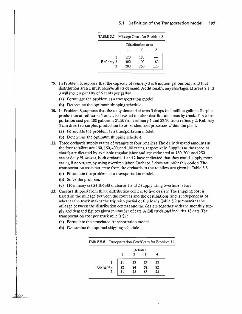
5.1 Definition of the Transportation Model 199
TABLE 5.7 Mileage Chart for Problem 8
Distribution area1 2 3
1Refinery 2
3
120300200
180100250
80120
*9. In Problem 8, suppose that the capacity of refinery 3 is 6 million gallons only and thatdistribution area 1 must receive all its demand. Additionally, any shortages at areas 2 and3 will incur a penalty of 5 cents per gallon.
(a) Formula,te the problem as a transportation model.
(b) Determine the optimum shipping schedule.
10. In Problem 8, suppose that the daily demand at area 3 drops to 4 million gallons. Surplusproduction at refineries 1 and 2 is diverted to other distribution areas by truck. The transportation cost per 100 gallons is $1.50 from refinery 1 and $2.20 from refinery 2. Refinery3 can divert its surplus production to other chemical processes within the plant.
(a) Formulate the problem as a transportation model.
(b) Determine the optimum shipping schedule.
11. Three orchards supply crates of oranges to four retailers. The daily demand amounts atthe four retailers are 150,150,400, and 100 crates, respectively. Supplies at the three orchards are dictated by available regular labor and are estimated at 150,200, and 250crates daily. However, both orchards 1 and 2 have indicated that they could supply morecrates, if necessary, by using overtime labor. Orchard 3 does not offer this option. Thetransportation costs per crate from the orchards to the retailers are given in Table 5.8.
(a) Formulate the problem as a transportation model.
(b) Solve the problem.
(c) How many crates should orchards 1 and 2 supply using overtime labor?
12. Cars are shipped from three distribution centers to five dealers. The shipping cost isbased on the mileage between the sources and the destinations, and is independent ofwhether the truck makes the trip with partial or full loads. Table 5.9 summarizes themileage between the distribution centers and the dealers together with the monthly supply and demand figures given in number of cars. A full truckload includes 18 cars. Thetransportation cost per truck mile is $25.
(a) Fonnulate the associated transportation model.
(b) Determine the optimal shipping schedule.
TABLE 5.8 Transportation Cost/Crate for Problem 11
II 1
Retailer2 3 4
1Orchard 2
3
$1$2$1
$2$4$3
$3$1$5
$2$2$3
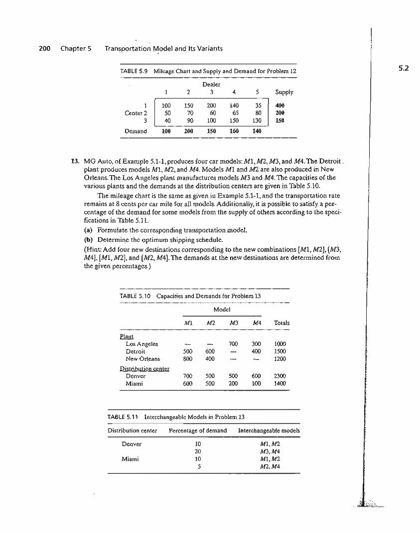
200 Chapter 5 Transportation Model and Its Variants
TABLE 5.9 Mileage Chart and Supply and Demand for Problem 12 5.2
Dealer1 2 3 4 5 Supply
1 100 150 200 140 35 400Center 2 50 70 60 65 80 200
3 40 90 100 150 130 150
Demand 100 200 150 160 140
13. MG Auto, of Example 5.1-1, produces four car models: MI, M2, M3, and M4. The Detroit.plant produces models Ml, M2, and M4. Models MI and M2 are also produced in NewOrleans. The Los Angeles plant manufactures models M3 and M4. The capacities of thevarious plants and the demands at the distribution centers are given in Table 5.10.
The mileage chart is the same as given in Example 5.1-1, and the transportation rateremains at 8 cents per car mile for all models. Additionally, it is possible to satisfy a percentage of the demand for some models from the supply of others according to the specifications in Table 5.11.(a) Formulate the corresponding transportation model.(b) Determine the optimum shipping schedule.
(Hint: Add four new destinations corresponding to the new combinations [MI, M2], [M3,M4], [Ml, M2], and [M2, M4]. The demands at the new destinations are determined fromthe given percentages.)
TABLE 5.10 Capacities and Demands for Problem 13
Model
M1 M2 M3 M4 Totals
PlantLos Angeles 700 300 1000Detroit 500 600 400 1500New Orleans 800 400 1200
Distribution centerDenver 700 500 500 600 2300Miami 600 500 200 100 1400
TABLE 5.11 Interchangeable Models in Problem 13
Distribution center
Denver
Miami
Percentage of demand
1020105
Interchangeable models
M1,M2M3,M4M1,M2M2,M4
", '-.:'... ;....:~..;~~..:...
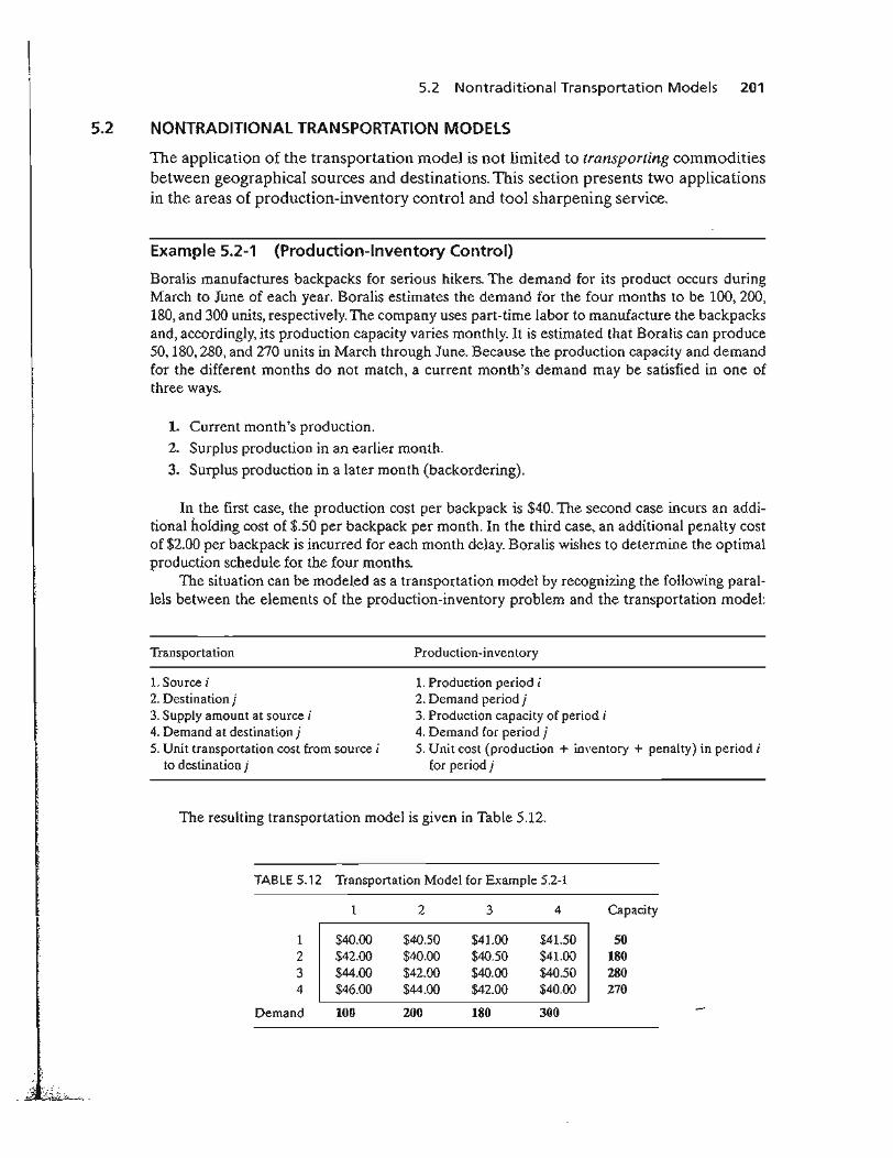
5.2 Nontraditional Transportation Models 201
5.2 NONTRADITIONAL TRANSPORTATION MODELS
The application of the transportation model is not limited to transporting commoditiesbetween geographical sources and destinations. This section presents two applicationsin the areas of production-inventory control and tool sharpening service.
Example 5.2-1 (Production-Inventory Control)
Boralis manufactures backpacks for serious hikers. The demand for its product occurs duringMarch to June of each year. Boralis estimates the demand for the four months to be 100, 200,180, and 300 units, respectively. The company uses part-time labor to manufacture the backpacksand, accordingly, its production capacity varies monthly. It is estimated that Boralis can produce50, 180,280, and 270 units in March through June. Because the production capacity and demandfor the different months do not match, a current month's demand may be satisfied in one ofthree ways.
1. Current month's production.
2. Surplus production in an earlier month.
3. Surplus production in a later month (backordering).
In the first case, the production cost per backpack is $40. The second case incurs an additional holding cost of $.50 per backpack per month. In the third case, an additional penalty costof $2.00 per backpack is incurred for each month delay. Boralis wishes to determine the optimalproduction schedule for the four months.
The situation can be modeled as a transportation model by recognizing the following parallels between the elements of the production-inventory problem and the transportation model:
Transportation
1. Source i2. Destination j3. Supply amount at source i4. Demand at destination j5. Unit transportation cost from source i
to destination j
Production-inventory
1. Production period i2. Demand period j3. Production capacity of period i4. Demand for period j5. Unit cost (production + inventory + penalty) in period i
for periodj
The resulting transportation model is given in Table 5.12.
TABLE 5.12 Transportation Model for Example 5.2-1
1 2 3 4 Capacity
1 $40.00 $40.50 $41.00 $41.50 502 $42.00 $40.00 $40.50 $41.00 1803 $44.00 $42.00 $40.00 $40.50 2804 $46.00 $44.00 $42.00 $40.00 270
Demand 100 200 180 300
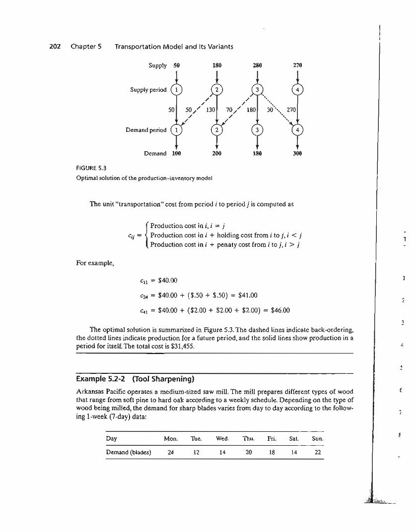
202 Chapter 5 Transportation Model and Its Variants
Supply 50 180 280 270
Supply period ...." .
30···•..".
Demand period
Demand 100 200 180 300
FIGURE 5.3
Optimal solution of the production-inventory model
The unit "transportation" cost from period i to period j is computed as
{
Production cost in i, i = j
eij = Production cost in i + holding cost from i to j, i < jProduction cost in i + penaty cost from i to j, i > j
1
For example,
Cll = $40.00
C24 = $40.00 + ($.50 + $.50) = $41.00
C41 == $40.00 + ($2.00 + $2.00 + $2.00) = $46.00
2
The optimal solution is summarized in Figure 5.3. The dashed lines indicate back-ordering,the dotted lines indicate production for a future period, and the solid lines show production in aperiod for itself. The total cost is $31,455. 4
Example 5.2-2 (Tool Sharpening)
Arkansas Pacific operates a medium-sized saw mill. The mill prepares different types of woodthat range from soft pine to hard oak according to a weekly schedule. Depending on the type ofwood being milled, the demand for sharp blades varies from day to day according to the following I-week (7-day) data:
7
Day Mon. The. Wed. 11m. Fri. Sat. Sun.
Demand (blades) 24 12 14 20 18 14 22
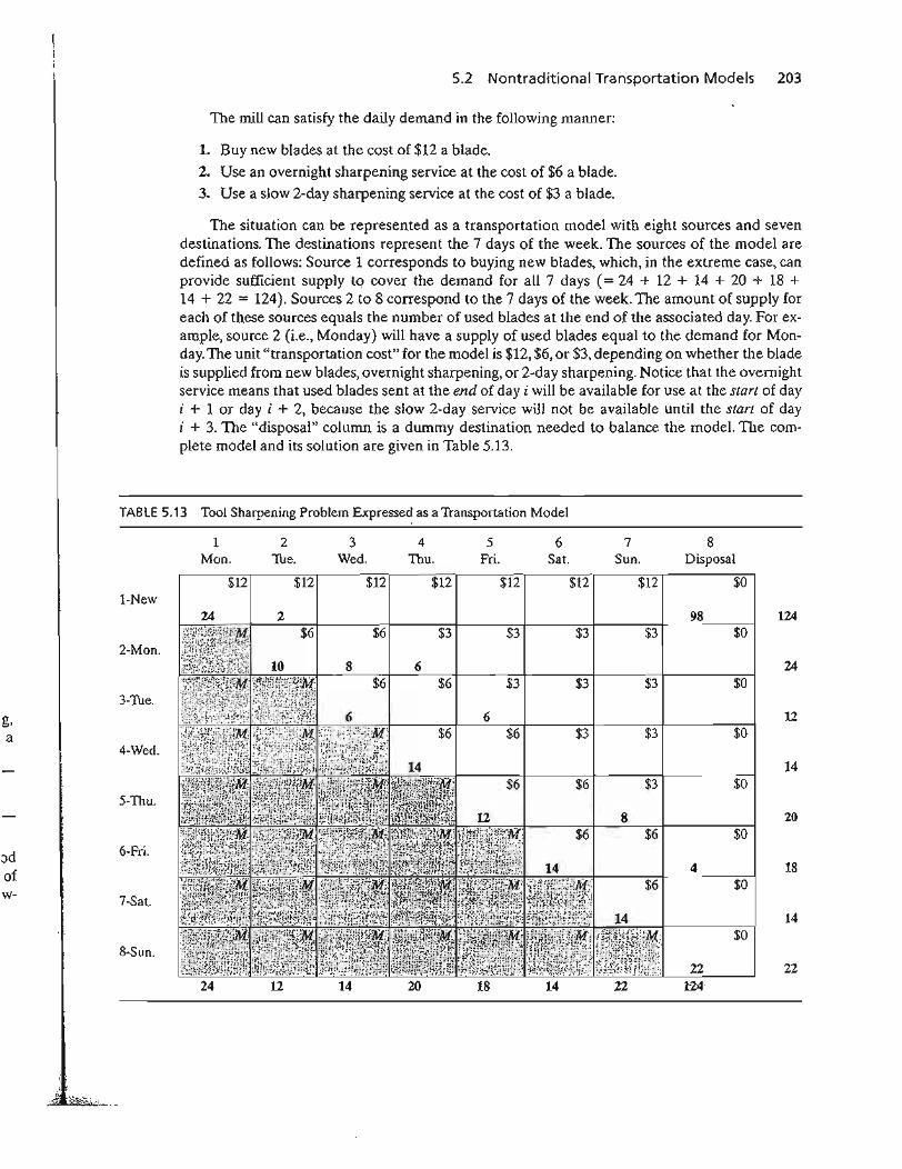
5.2 Nontraditional Transportation Models 203
The mill can satisfy the daily demand in the following manner:
1. Buy new blades at the cost of $12 a blade.
2. Use an overnight sharpening service at the cost of $6 a blade.
3. Use a slow 2-day sharpening service at the cost of $3 a blade.
The situation can be represented as a transportation model with eight sources and sevendestinations. The destinations represent the 7 days of the week. The sources of the model aredefined as follows: Source 1 corresponds to buying new blades, which, in the extreme case, canprovide sufficient supply to cover the demand for all 7 days (= 24 + 12 + 14 + 20 + 18 +14 + 22 = 124). Sources 2 to 8 correspond to the 7 days of the week. The amount of supply foreach of these sources equals the number of used blades at the end of the associated day. For example, source 2 (i.e., Monday) will have a supply of used blades equal to the demand for Monday. The unit "transportation cost" for the model is $12, $6, or $3, depending on whether the bladeis supplied from new blades, overnight sharpening, or 2-day sharpening. Notice that the overnightservice means that used blades sent at the end of day i will be available for use at the start of dayi + 1 or day i + 2, because the slow 2-day service will not be available until the start of dayi + 3. The "disposal" column is a dummy destination needed to balance the model. TIle complete model and its solution are given in Table 5.13.
TABLE 5.13 Tool Sharpening Problem Expressed as a Transportation Model
5-Thu.
Jd 6·Fri.
ofw- 7-Sat.
8-Sun.
$12
8Disposal
$0
98 124$0
24$0
12$0
14$0
20$0
22
14
18$0
$0
4
22
$3
$3
$12
$3
7Sun.
22
$3
$12
$3
$3
6Sat.
14
$6
$3
$3
6
5Fri.
18
$12
6$6
$3
$6
4Thu.
14
$6
$12
$6
6
8
3Wed.
14
$12
2
2Tue.
12
1Mon.
24
$12
24
2-Mon.
4-Wed.
3-Tue.
1-New
g,a
204 Chapter 5 Transportation Model and Its Variants
The problem has alternative optima at a cost of $840 (file toraExS.2-2.txt).The following tablesummarizes one such solution.
Number of sharp blades (Target day)
peri1 New Overnight 2-day Disposal
Mon. 24 (Mon.) lO(Tue.) + 8{Wed.) 6 (Thu.) 0Tues. 2 (Tue.) 6 (Wed.) 6 (Fri.) 0Wed. 0 14 (11lU.) 0 011lU. 0 12 (Fri.) 8 (Sun.) 0Fri. 0 14 (Sat.) 0 4Sat. 0 14 (Sun.) 0 0Sun. 0 0 0 22
Remarks. The model in Table 5.13 is suitable only for the first week of operation because itdoes not take into account the rotational nature of the days of the week, in the sense that thisweek's days can act as sources for next week's demand. One way to handle this situation is to assume that the very first week of operation starts with all new blades for each day. From then on,we use a model consisting of exactly 7 sources and 7 destinations corresponding to the days ofthe week. The new model will be similar to Table 5.13 less source "New" and destination "Disposal." Also, only diagonal cells will be blocked (unit cost = M). The remaining cells will have aunit cost of either $3.00 or $6.00. For example, the unit cost for cell (Sat., Mon.) is $6.00 and thatfor cells (Sat., Tue.), (Sat., Wed.), (Sat., Thu.), and (Sat., Fri.) is $3.00. The table below gives thesolution costing $372. As expected, the optimum solution will always use the 2-day service only.TIle problem has alternative optima (see file toraEx5.2-2a.txt).
Weeki
Mon.Tue.Wed.TIm.Fri.Sat.Sun.Total
Mon.
1284
24
Tue.
12
12
Week i + 1
Wed. Thu. Fri. Sal. Sun. Total
6 18 248 4 12
2 1420
14 1814 14
10 12 2214 20 18 14 22
PROBLEM SET S.2A3
1. In Example 5.2-1, suppose that the holding cost per unit is period-dependent and is givenby 40, 30, and 70 cents for periods 1,2, and 3, respectively. The penalty and productioncosts I'emain as given in the example. Determine the optimum solution and interpretthe results.
3In this set, you may use TORA to find the optimum solution. AMPL and Solver models for the transportation problem will be introduced at the end of Section 5.3.2.
5.2 Nontraditional Tr"ansportation Models 205
*2. In Example 5.2-2, suppose that the sharpening service offers 3-day service for $1 a bladeon Monday and Tuesday (days 1 and 2). Reformulate the problem, and interpret the optimum solution.
3. In Example 5.2-2, if a blade is not used the day it is sharpened, a holding cost of 50 centsper blade per day is incurred. Reformulate the model, and interpret the optimum solution.
4. JoShop wants to assign four different categories of machines to five types of tasks. Thenumbers of machines available in the four categories are 25, 30,20, and 30. The numbersof jobs in the five tasks are 20, 20, 30,10, and 25. Machine category 4 cannot be assignedto task type 4. Table 5.14 provides the unit cost (in dollars) of assigning a machine category to a task type. The objective of the problem is to determine the optimum number ofmachines in each category to be assigned to each task type. Solve the problem and interpret the solution.
*5. The demand for a perishable item over the next four months is 400,300,420, and 380tons, respectively. The supply capacities for the same months are 500, 600, 200, and 300tons. The purchase price per ton varies from month to month and is estimated at $100,$140, $120, and $150, respectively. Because the item is perishable, a current month's supply must be consumed within 3 months (starting with current month). The storage costper ton per month is $3. The nature of the item does not allow back-ordering, Solve theproblem as a transportation model and determine the optimum delivery schedule for theitem over the next 4 months.
6. The demand for a special small engine over the next five quarters is 200, 150, 300,250,and 400 units. The manufacturer supplying the engine has different production capacitiesestimated at 180,230,430,300, and 300 for the five quarters. Back-ordering is not allowed, but the manufacturer may use overtime to fill the immediate demand, if necessary.The overtime capacity for each period is half the regular capacity. The production costsper unit for the five periods are $100, $96, $116, $102, and $106, respectively. TIle overtime production cost per engine is 50% higher than the regular production cost. If an engine is produced now for use in later periods, an additional storage cost of $4 per engineper period is incurred. Formulate the problem as a transportation model. Determine theoptimum number of engines to be produced during regular time and overtime of eachperiod.
7. Periodic preventive maintenance is carried out on aircraft engines, where an importantcomponent must be replaced. The numbers of aircraft scheduled for such maintenanceover the next six months are estimated at 200, 180,300,198,230, and 290, respectively. Allmaintenance work is done during the first day of the month, where a used componentmay be replaced with a new or an overhauled component. The overhauling of used components may be done in a local repair facility, where they will be ready for use at the beginning of next month, or they may be sent to a central repair shop, where a delay of
TABLE 5.14 Unit Costs for Problem 4
Task type1 2 3 4 5
1 10 2 3 15 9
Machine category2 5 10 15 2 43 15 5 14 7 154 20 15 13 8
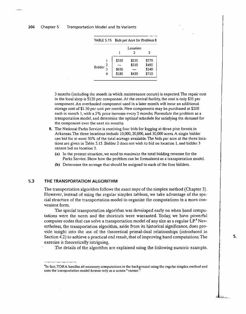
206 Chapter 5 Transportation Model and Its Variants
TABLE 5.15 Bids per Acre for Problem 8
Location1 2 3
1 $520 $210 $570. d 2 $510 $495
Bid er 3 $650 $2404 $180 $430 $710
3 months (including the month in which maintenance occurs) is expected. The repair costin the local shop is $120 per component. At the central facility, the cost is only $35 percomponent. An overhauled component used in a later month will incur an additionalstorage cost of $1.50 per unit per month. New components may be purchased at $200each in month 1, with a 5% price increase every 2 months. Formulate the problem as atransportation model, and determine the optimal schedule for satisfying the demand forthe component over the next six months.
8. The National Parks Service is receiving four bids for logging at three pine forests inArkansas. The three locations include 10,000,20,000, and 30,000 acres. A single biddercan bid for at most 50% of the total acreage available. The bids per acre at the three locations are given in Table 5.15. Bidder 2 does not wish to bid on location I, and bidder 3cannot bid on location 2.
(a) In the present situation, we need to maximize the total bidding revenue for theParks Service. Show how the problem can be formulated as a transportation model.
(b) Determine the acreage that should be assigned to each of the four bidders.
5.3 THE TRANSPORTATION ALGORITHM
The transportation algorithm follows the exact steps of the simplex method (Chapter 3).However, instead of using the regular simplex tableau, we take advantage of the special structure of the transportation model to organize the computations in a more convenient form.
The special transportation algorithm was developed early on when hand computations were the norm and the shortcuts were warranted. Today, we have powerfulcomputer codes that can solve a transportation model of any size as a regular Lp'4 Nevertheless, the transportation algorithm, aside from its historical significance, does provide insight into the use of the theoretical primal-dual relationships (introduced inSection 4.2) to achieve a practical end result, that of improving hand computations. TIleexercise is theoretically intriguing.
The details of the algorithm are explained using the following numeric example.
4In fact, TORA handles all necessary computations in the background using the regular simplex method anduses the transportation model format only as a screen "veneer."
5.
5.3 The Transportation Algorithm 207
TABLE 5.16 SunRay Transportation Model
Mill1 2 3 4 Supply
1
Silo2.
3
10 2 20 11
Xli Xl2 XI3 X\4
12 7 9 20
X2l X22 X23 X24
4 14 16 18
X31 X32 X33 X 34
15
25
10
Demand 5 15 15 15
I.:-
l-
l
Il{
)
Inle
.e.
nd
. _.., ':.iI:'..:.;,,~._.
Example 5.3-1 (SunRay Transport)
SunRay Transport Company ships truckloads of grain from three silos to four mills. The supply(in truckloads) and the demand (also in truckloads) together with the unit transportation costsper truckload on the different routes are summarized in the transportation model in Table 5.16.The unit transportation costs, eij, (shown in the northeast corner of each box) are in hundreds ofdollars. The model seeks the minimum-cost shipping schedule Xij between silo i and mill j(i = 1,2,3;j = 1,2,3,4).
Summary of the Transportation Algorithm. The steps of the transportation algorithmare exact parallels of the simplex algorithm.
Step 1. Determine a starting basic feasible solution, and go to step 2.Step 2. Use the optimality condition of the simplex method to determine the
entering variable from among all the nonbasic variables. If the optimalitycondition is satisfied, stop. Otherwise, go to step 3.
Step 3. Use the feasibility condition of the simplex method to determine the leavingvariable from among all the current basic variables, and find the new basic solution. Return to step 2.
5.3.1 Determination of the Starting Solution
A general transportation model with m sources and n destinations has m + n constraintequations, one for each source and each destination. However, because the transportation model is always balanced (sum of the supply = sum of the demand), one of theseequations is redundant. Thus, the model has m + n - 1 independent constraint equations, which means that the starting basic solution consists of m + n - 1 basic variables.Thus, in Example 5.3-1, the starting solution has 3 + 4 - 1 = 6 basic variables.
208 Chapter 5 Transportation Model and Its Variants
The special structure of the transportation problem allows securing a nonartificiaI starting basic solution using one of three methods:5
1. Northwest-corner method2. Least-cost method3. Vogel approximation method
. The three methods differ in the "quality" of the starting basic solution they produce, inthe sense that a better starting solution yields a smaller objective value. In general,though not always, the Vogel method yields the best starting basic solution, and thenorthwest-corner method yields the worst. The tradeoff is that the northwest-cornermethod involves the least amount of computations.
Northwest-Corner Method. The method starts at the northwest-corner cell (route) ofthe tableau (variable xu).
Step 1. Allocate as much as possible to the selected cell, and adjust the associatedamounts of supply and demand by subtracting the allocated amount.
Step 2. Cross out the row or column with zero supply or demand to indicate that nofurther assignments can be made in that row or column. If both a row and acolumn net to zero simultaneously, cross out one only, and leave a zero supply (demand) in the uncrossed-out TOW (column).
Step 3. If exactly one row or column is left uncrossed out, stop. Otherwise, move tothe cell to the right if a column has just been crossed out or below if a row hasbeen crossed out. Go to step 1.
Example 5.3-2
The application of the procedure to the model of Example 5.3-1 gives the starting basic solutionin Table 5.17. The arrows show the order in which the allocated amounts are generated.
The starting basic solution is
Xu = 5, X12 = 10
X22 = 5, X23 = 15, X24 = 5
XJ4 = 10
The associated cost of the schedule is
z = 5 X 10 + 10 X 2 + 5 X 7 + 15 X 9 + 5 X 20 + 10 X 18 = $520
Least-Cost Method. The least-cost method finds a better starting solution byconcentrating on the cheapest routes. The method assigns as much as possible to thecell with the smallest unit cost (ties are broken arbitrarily). Next, the satisfied row orcolumn is crossed out and the amounts of supply and demand are adjusted accordingly.
5All three methods are featured in TORA's tutorial module. See the end of Section 5.3.3.
5.3 The Transportation Algorithm 209
TABLE 5.17 Northwest-Corner Starting Solution
1 2 3 4 Supply
1
2
3
10 2 20 11
;;i~,~-----"~5~~)1 15
25
10
Demand 5 15 15 15
)
s
n
Jyleorly.
If both a row and a column are satisfied simultaneously, only one is crossed out, thesame as in the northwest-corner method. Next, look for the uncrossed-out cell withthe smallest unit cost and repeat the process until exactly one row or column is leftuncrossed out.
Example 5.3-3
The least-cost method is applied to Example 5.3-1 in the following manner:
1. Cell (1, 2) has the least unit cost in the tableau (= $2). The most that can be shippedthrough (1,2) is X12 = 15 truckloads, which happens to satisfy both row 1 and column 2 si·multaneously. We arbitrarily cross out column 2 and adjust the supply in row 1 to O.
2. Cell (3,1) has the smallest uncrossed-out unit cost (= $4). Assign X31 = 5, and cross outcolumn 1 because it is satisfied, and adjust the demand of row 3 to 10 - 5 = 5 truckloads.
3. Continuing in the same manner, we successively assign 15 truckloads to cell (2, 3),o truckloads to cell (1,4), 5 truckloads to cell (3, 4), and 10 truckloads to cell (2,4)(verify!).
The resulting starting solution is summarized in Table 5.18. The arrows show the order inwhich the allocations are made. The starting solution (consisting of 6 basic variables) isx12 = 15, X14 = 0, X23 = 15, X24 = 10, X31 = 5, X34 = 5. The associated objective value is
z = 15 X 2 + 0 x 11 + 15 x 9 + 10 x 20 + 5 x 4 + 5 x 18 = $475
The quality of the least-cost starting solution is better than that of the northwestcorner method (Example 5.3-2) because it yields a smaller value of z ($475 versus $520in the northwest-corner method).
Vogel Approximation Method (VAM). VAM is an improved version of the least-costmethod that generally, but not always, produces better starting solutions.
Step 1. For each row (column), determine a penalty measure by subtracting thesmallest unit cost element in the row (column) from the next smallest unitcost element in the same row (column).
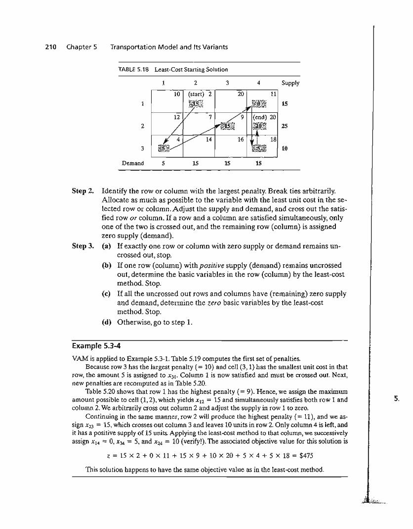
210 Chapter 5 Transportation Model and Its Variants
TABLE 5.18 Least-Cost Starting Solution
1 2 3 4 Supply
10 (start) 2 20 11
1 ~Em 15
2 25
18
3 10
Demand 5 15 15 15
Step 2. Identify the row or column with the largest penalty. Break ties arbitrarily.Allocate as much as possible to the variable with the least unit cost in the selected row or column. Adjust the supply and demand, and cross out the satisfied row or column. If a row and a column are satisfied simultaneously, onlyone of the two is crossed out, and the remaining row (column) is assignedzero supply (demand).
Step 3. (a) If exactly one row or column with zero supply or demand remains uncrossed out, stop.
(b) If one row (column) with positive supply (demand) remains uncrossedout, determine the basic variables in the row (column) by the least-costmethod. Stop.
(c) If all the uncrossed out rows and columns have (remaining) zero supplyand demand, determine the zero basic variables by the least-costmethod. Stop.
(d) Otherwise, go to step 1.
Example 5.3-4
VAM is applied to Example 5.3-1. Table 5.19 computes the first set of penalties.Because row 3 has the largest penalty (= 10) and cell (3, 1) has the smallest unit cost in that
row, the amount 5 is assigned to x31' Column 1 is now satisfied and must be crossed out. Next,new penalties are recomputed as in Table 5.20.
Table 5.20 shows that row 1 has the highest penalty (= 9). Hence, we assign the maximumamount possible to cell (1,2), which yields Xt2 = 15 and simultaneously satisfies both row 1 andcolumn 2. We arbitrarily cross out column 2 and adjust the supply in row 1 to zero.
Continuing in the same manner, row 2 will produce the highest penalty (= 11), and we assign X23 = 15, which crosses out column 3 and leaves 10 units in row 2. Only column 4 is left, andit has a positive supply of 15 units. Applying the least-cost method to that column, we successivelyassign X14 = 0, X34 = 5, and X24 = 10 (verify!). The associated objective value for this solution is
z = 15 x 2 + 0 x 11 + 15 x 9 + 10 x 20 + 5 x 4 + 5 x 18 = $475
This solution happens to have the same objective value as in the least-cost method.
._.::.~_._-
5.
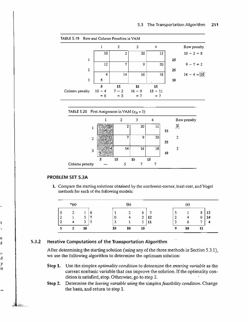
5.3 The Transportation Algorithm 211
TABLE 5.19 Rowand Column Penalties in YAM
1
10 2 20 11
12 7 9 20
4 14 16 185
1
2
3
5Column penalty 10 - 4
= 6
2
157-2
=5
3
1516 - 9
=7
4
1518 - 11
=7
15
25
10
Row penalty
10-2=8
9-7=2·
14 - 4 =&im
TABLE 5.20 First Assignment in VAM (X31 ;; 5)
1 2
5 15Column penalty
3 4 Row penalty
2 20 11 i9.';15
7 9 20 22S
14 16 18 210
15 155 7 7
PROBLEM SET 5.3A
1. Compare the starting solutions obtained by the northwest-comer, least-cost, and Vogelmethods for each of the following models:
*(a) (b) (c)
0 2 1 6 1 2 6 7 5 1 8 122 1 5 7 0 4 2 12 2 4 0 14
t 2 4 3 7 3 1 5 11 3 6 7 4
5 S 10 10 10 10 9 10 11
(1
d 5.3.2
j-
dyis
Iterative Computations of the Transportation Algorithm
After determining the starting solution (using any of the three methods in Section 5.3.1),we use the following algorithm to determ~ne the optimum solution:
Step 1. Use the simplex optimality condition to determine the entering variable as thecurrent nonbasic variable that can improve the solution. If the optimality condition is satisfied, stop. Otherwise, go to step 2.
Step 2. Determine the leaving variable using the simplex feasibility condition. Changethe basis, and return to step 1.
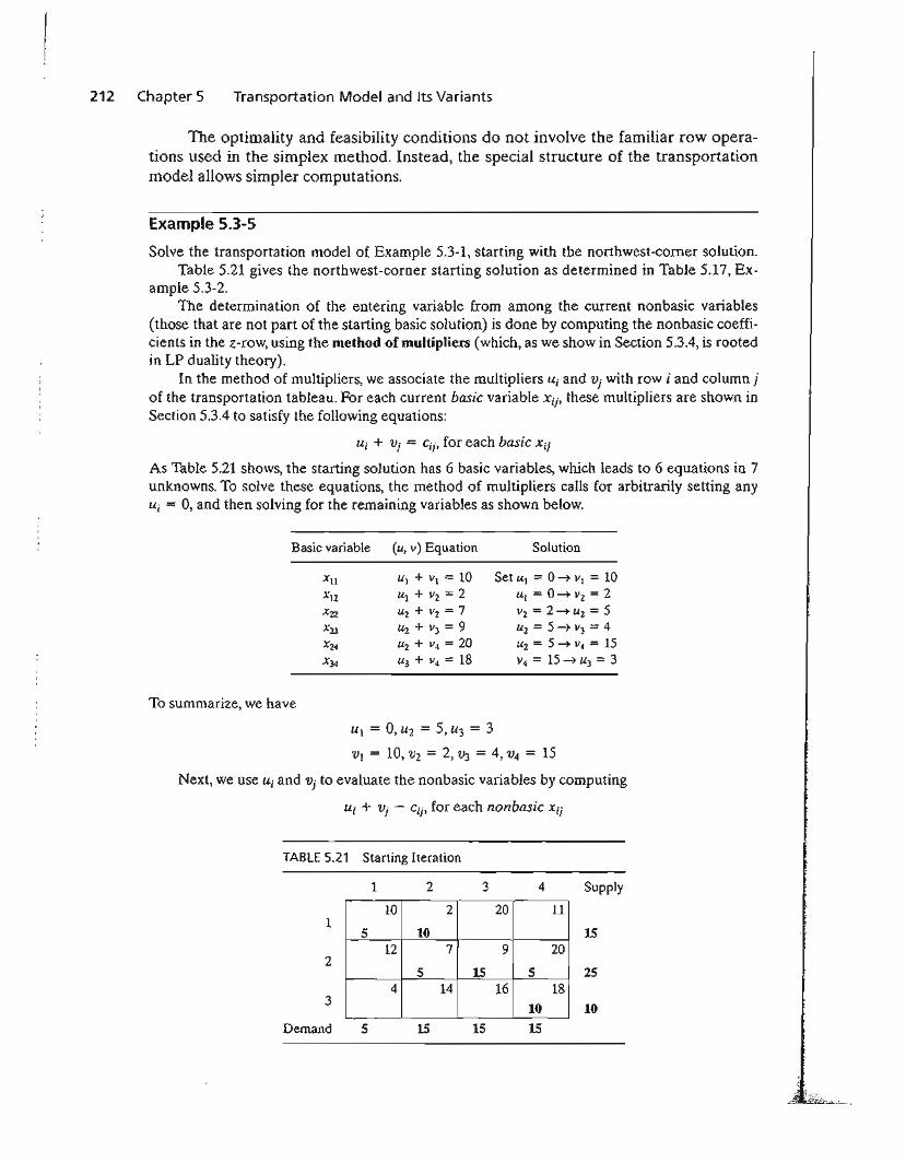
212 Chapter 5 Transportation Model and Its Variants
The optimality and feasibility conditions do not involve the familiar row operations used in the simplex method. Instead, the special structure of the transportationmodel allows simpler computations.
Example 5.3-5
Solve the transportation model of Example 5.3-1, starting with the northwest-corner solution.Table 5.21 gives the northwest-corner starting solution as determined in Table 5.17, Ex
ample 5.3-2.The determination of the entering variable from among the current nonbasic variables
(those that are not part of the starting basic solution) is done by computing the nonbasic coefficients in the z-row, using the method of multipliers (which, as we show in Section 5.3.4, is rootedin LP duality theory).
In the method of multipliers, we associate the multipliers Ui and v; with row i and column jof the transportation tableau. For each current basic variable Xi;, these multipliers are shown inSection 5.3.4 to satisfy the following equations:
Ui + v; = Cij, for each basic Xij
As Table 5.21 shows, the starting solution has 6 basic variables, which leads to 6 equations in 7unknowns. To solve these equations, the method of multipliers calls for arbitrarily setting anyUi = 0, and then solving for the remaining variables as shown below.
Basic variable
To summarize, we have
(u, v) Equation
Ul + VI = 10UI + Vz = 2Uz + Vz = 7U2 + v3 = 9til + V4 = 20U3 + V4 = 18
Solution
Set Ul = 0~ VI = 10UI = 0~V2 = 2Vl = 2~ul = 5Uz = 5~ V3 = 4U2 = 54> V4 = 15V4 = 15~ U3 = 3
Ul = 0, u2 = 5, U3 = 3
VI = 10, V2 = 2, V3 = 4, V4 = 15
Next, we use Ui and Vj to evaluate the nonbasic variables by computing
Ui + Vj - Cij, for each nonbasic Xi;
TABLE 5.21 Starting Iteration
1 2 3 4 Supply
1
2
3
10 2 20 11
5 1012 7 9 20
5 15 54 14 16 18
10
15
25
10Demand 5 15 15 15
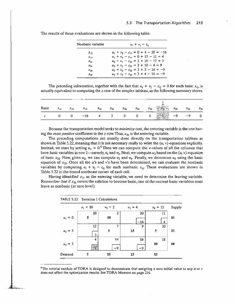
5.3 The Transportation Algorithm 213
The results of these evaluations are shown in the following table:
Nonbasic variable
Ul + VJ - Cn = 0 + 4 - 20 = -16UI + V4 - Cl4 = 0 + 15 - 11 = 4Uz + VI - CZl = 5 + 10 - 12 = 3UJ + VJ - C31 = 3 + 10 - 4 = 9U3 + Vz - C3Z = 3 + 2 - 14 = -9UJ + V3 - CJ3 = 3 + 4 - 16 = -9
The preceding information, together with the fact that Ui + vi - eli = 0 for each basic xii' isactually equivalent to computing the z-row of the simplex tableau, as the following summary shows.
~Basic Xli X12 XIJ X14 X21 X22 XZ3 XZ4 :~~t~t~:r::~j X32 X33 X34
Z 0 0 -16 4 3 0 0 0 f,t.1.F&2~Y~ -9 -9 0
Because the transportation model seeks to minimize cost, the entering variable is the one having the most positive coefficient in the z-row. Thus, x31 is the entering variable.
The preceding computations are usually done directly on the transportation tableau asshown in Table 5.22, meaning that it is not necessary really to write the (u, v)-equations explicitly.Instead, we start by setting Ul = 0.6 Then we can compute the v-values of all the columns thathave basic variables in row I-namely, VI and V2' Next, we compute U2 based on the (u, v)-equationof basic Xzz. Now, given Uz, we can compute VJ and V4' Finally, we determine U3 using the basicequation of X33. Once all the u's and v's have been determined, we can evaluate the nonbasicvariables by computing Ui + Vi ~ cii for each nonbasic Xii" These evaluations are shown inTable 5.22 in the boxed southeast corner of each cell.
Having identified X31 as the entering variable, we need to detennine the leaving variable.Remember that if X31 enters the solution to become basic, one of the current basic variables mustleave as nonbasic (at zero level).
TABLE 5.22 Iteration 1 Calculations
V2 = 2 Supply
Uz = 5
10 2 20 115 10
r=M ~12 7 9 20
r-;- 5 15 5
4 14 16 18
~, H r=910
15
25
10
Demand 5 15 15 15
6The tutorial module ofTORA is designed to demonstrate that assigning a zero initial value to any a or V
does not affect the optimization results. See TORA Moment on page 216.
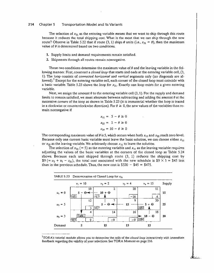
214 Chapter 5 Transportation Model and Its Variants
The selection of X31 as the entering variable means that we want to ship through this routebecause it reduces the total shipping cost. What is the most that we can ship through the newroute? Observe in Table 5.22 that if route (3, 1) ships () units (i.e., X31 = e), then the maximumvalue of () is determined based on two conditions.
1. Supply limits and demand requirements remain satisfied.
2. Shipments through all routes remain nonnegative.
These two conditions determine the maximum value of () and the leaving variable in the following manner. First, construct a closed loop that starts and ends at the entering variable cell, (3,1). The loop consists of connected horizontal and vertical segments only (no diagonals are allowed).7 Except for the entering variable cell, each corner of the closed loop must coincide witha basic variable. Table 5.23 shows the loop for X31' Exactly one loop exists for a given enteringvariable.
Next, we assign the amount e to the entering variable cell (3, 1). For the supply and demandlimits to remain satisfied, we must alternate between subtracting and adding the amount eat thesuccessive corners of the loop as shown in Table 5.23 (it is immaterial whether the loop is tracedin a clockwise or counterclockwise direction). For e ~ 0, the new values of the variables then remain nonnegative if
XIl::= 5 - e ~ 0
Xn = 5 - (} 2: 0
X34 = 10 - e ~ 0
The corresponding maximum value of () is 5, which occurs when both Xu and X22 reach zero level.Because only one current basic variable must leave the basic solution, we can choose either Xu
or X22 as the leaving variable. We arbitrarily choose Xu to leave the solution.The selection of X31 (:= 5) as the entering variable and Xu as the leaving variable requires
adjusting the values of the basic variables at the corners of the closed loop as Table 5.24shows. Because each unit shipped through route (3, 1) reduces the shipping cost by$9 (= U3 + VI - C31)' the total cost associated with the new schedule is $9 X 5 := $45 lessthan in the previous schedule. Thus, the new cost is $520 - $45 = $475.
TABLE 5.23 Determination of Closed Loop for x31
Supply
-16 4
10 25 - e---E.-- .-.. 10 + e
~t#~~~ :¥~~ 1
20 1115
25
10
9 20-..--. --"-- 5 + e
~~~~~ 116 18
..---.---...-...---. ~ 10 - e-9 *~~
14
12 75 - e ~.- -..-.- 15
~~:l~f.~fl~\i .--.~-- .- -._- _~~.
Demand 5 15 15 15
7TORA's tutorial module allows you to determine the cells of the closed loop interactively with immediatefeedback regarding the validity of your selections. See TORA Moment on page 216.
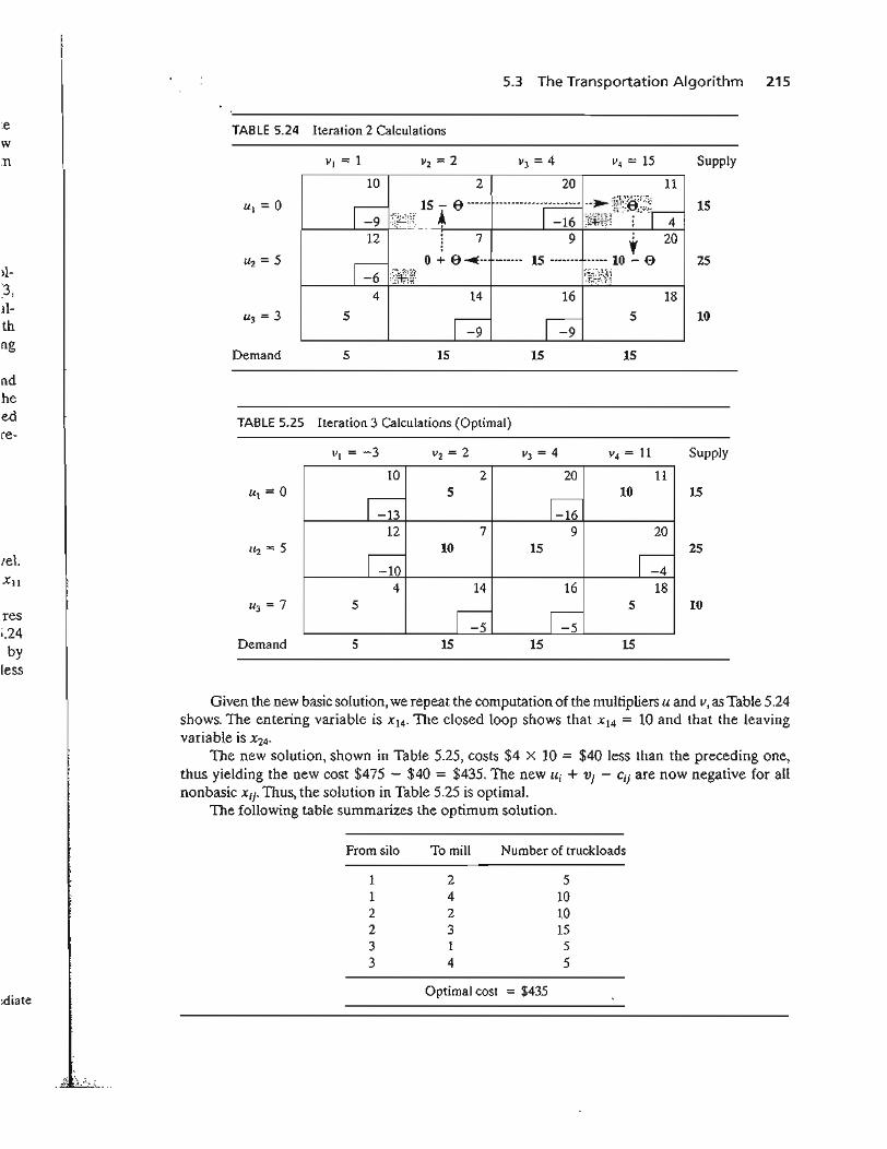
5.3 The Transportation Algorithm 215
:ewn
TABLE 5.24 Iteration 2 Calculations
Supply
25
1018
5
15
16
15
14
15
4
10 2 20 11
r=; ~:;;pn 15 ~ e ------ -------·-·-·~;~~~tli::~;;T__4 15
12 7 9, 20
o + e ....-- 15 -..---- ------ 10 - er=6':%~i
5
5Demand
>13,lIthrlg
rldheedre-
TABLE 5-25 Iteration 3 Calculations (Optimal)
Vz = 2 Supply
10 2 20 11
r=-;5
~10
12 7 9 20
~10 15
~4 14 16 18
5
~ ~5
u, == 0
Uz = 5leI.Xu
U3 = 7res;.24by Demand
less
5 15 15 15
15
25
10
Given the new basic solution, we repeat the computation of the multipliers u and v, as Table 5.24shows. The entering variable is X14. The closed loop shows that X14 = 10 and that the leavingvariable is XZ4'
The new solution, shown in Table 5.25, costs $4 X 10 = $40 less than the preceding one,thus yielding the new cost $475 - $40 = $435. The new Ui + Vj - Cij are now negative for allnonbasic Xij' Thus, the solution in Table 5.25 is optimal.
The following table summarizes the optimum solution.
From silo To mill Number of truckloads
1 2 51 4 102 2 102 3 153 1 53 4 5
:diateOptimal cost = $435
216 Chapter 5 Transportation Model and Its Variants
TORA Moment.
From~b!Y~/Mo~i.fY:M~iiti!,select :$()lV#: => :~i~i.~!!Qg~:j, and choose one of the threemethods (~o~-th~e;£corner,least-cost, or Vogel) to start the transportation model iterations. The iterations module offers two useful interactive features:
1. You can set any U or v to zero before generating Iteration 2 (the default is Ul = 0).Observe then that although the values of Ui and Vj change, the evaluation of thenonbasic cells (= Uj + Vj - Cij) remains the same.This means that, initially, any U orv can be set to zero (in fact, any value) without affecting the optimality calculations.
2. You can test your understanding of the selection of the closed loop by clicking (inany order) the corner cells that comprise the path. If your selection is correct, thecell will change color (green for entering variable, red for leaving variable, andgray otherwise).
Solver Moment.
Entering the transportation model into Excel spreadsheet is straightforward. Figure 5.4provides the Excel Solver template for Example 5.3-1 (file solverEx5.3-l.xls), togetherwith all the formulas and the definition of range names.
In the input section, data include unit cost matrix (cells B4:E6), source names(cells A4:A6), destination names (cells B3:E3), supply (cells F4:F6), and demand (cellsB7:E7). In the output section, cells Bll:E13 provide the optimal solution in matrixform. The total cost formula is given in target cell AIO.
AMPl Moment.
Figure 5.5 provides the AMPL model for the transportation model of Example 5.3-1(file amplEx5.3-1a.txt). The names used in the model are self-explanatory. Both theconstraints and the objective function follow the format of the LP model presented inExample 5.1-I.
The model uses the sets sNodes and dNodes to conveniently allow the use of thealphanumeric set members {51, 52, 53} and {Dl, D2, D3, D4} which are enteredin the data section. All the input data are then entered in terms of these set members asshown in Figure 5.5.
Although the alphanumeric code for set members is more readable, generatingthem for large problems may not be convenient. File ampIExS.3-1b shows how thesame sets can be defined as {1 .. m) and {1 .. n}, where m and n represent the numberof sources and the number of destinations. By simply assigning numeric values for In
and n, the sets are automatically defined for any size model.The data of the transportation model can be retrieved from a spreadsheet (file
TM.x1s) using the AMPL table statement. File amplEx3S1c.txt provides the details.To study this model, you will need to review the material in Section A.5.S.
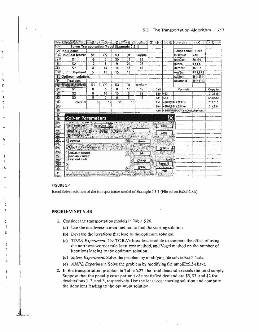
I.
r
1
i
~
r
5
5
I{
L
1
j
5
rn
5.3 The Transportation Algorithm 217
FIGURE 5.4
Excel Solver solution of the transportation model of Example 5.3-1 (File solverEx5.3-1.xls)
PROBLEM SET 5.3B
1. Consider the transportation models in Table 5.26.
(a) Use the northwest-corner method to find the starting solution.
(b) Develop the iterations that lead to the optimum solution.
(c) TORA Experiment. Use TORA's Iterations module to compare the effect of usingthe northwest-corner rule, least-cost method, and Vogel method on the number ofiterations leading to the optimum solution.
(d) Solver Experiment. Solve the problem by modifying file solverEx5.3-l.xls.
(e) AMPL Experiment. Solve the problem by modifying file ampIEx5.3-lb.txt.
2. In the transportation problem in Table 5.27, the total demand exceeds the total supply.Suppose that the penalty costs per unit of unsatisfied demand are $5, $3, and $2 fordestinations 1,2, and 3, respectively. Use the least-cost starting solution and computethe iterations leading to the optimum solution.
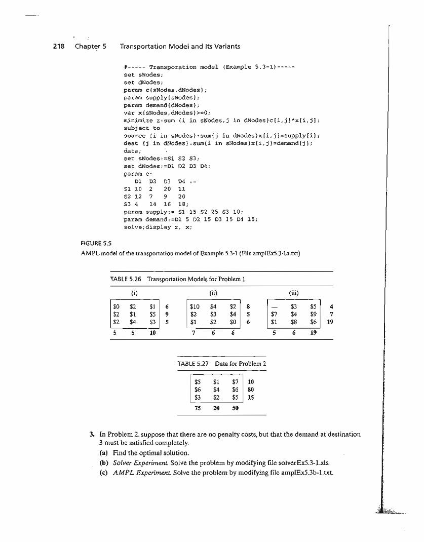
218 Chapt~r 5 Transportation Model and Its Variants
#----- Transporation model (Example 5.3-1)----set sNodes;set dNodes;param c{sNodes,dNodes);param supply{sNodes};param demand{dNodes};var x{sNodes,dNodes}>~O;
minimize z:sum {i in sNodes,j in dNodes}c[i,j]*x[i,j];subject tosource {i in sNodes}:sum{j in dNodes}x[i,jj=supply[i];dest {j in dNodes}:sum{i in sNodes}x[i,j]=demand[j];data;set sNodes:=Sl S2 S3;set dNodes:=D1 D2 D3 D4;param c:
Dl D2 D3 D4 .SIlO 2 20 11S2 12 7 9 20S3 4 14 16 18;param supply:= SI 15 S2 25 S3 10;param demand:=Dl 5 D2 15 D3 15 D4 15;solve;display z, x;
FIGURE 5.5
AMPL model of the transportation model of Example 5.3-1 (File ampIEx5.3-1a.txt)
TABLE 5.26 Transportation Models for Problem 1
(i) (ii) (iii)
$0 $2 $1 6 $10 $4 $2 8 $3 $5 4$2 $1 $5 9 $2 $3 $4 5 $7 $4 $9 7$2 $4 $3 5 $1 $2 $0 6 $1 $8 $6 19
5 5 10 7 6 6 5 6 19
TABLE 5.27 Data for Problem 2
$5 $1 $7 10$6 $4 $6 80$3 $2 $5 15
75 20 50
3. In Problem 2, suppose that there are no penalty costs, but that the demand at destination3 must be satisfied completely.
(a) Find the optimal solution.
(b) Solver Experiment. Solve the problem by modifying file solverExS.3-l.xls.(c) AMPL Experiment. Solve the problem by modifying file ampIEx5.3b-l.txt.
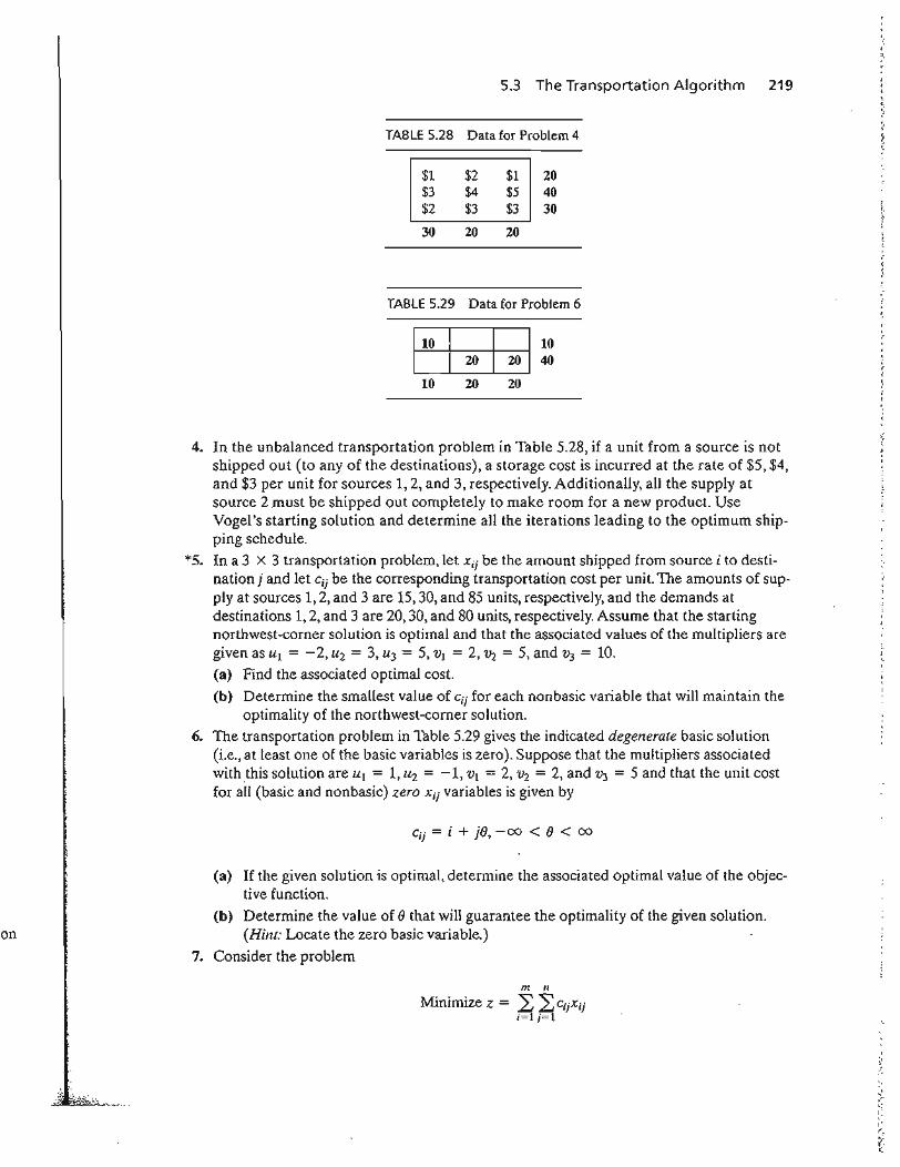
on
5.3 The Transportation Algorithm 219
TABLE 5.28 Data for Problem 4
$1 $2 $1 20$3 $4 $5 40$2 $3 $3 30
30 20 20
TABLE 5.29 Data for Problem 6
~:10 20 20
4. In the unbalanced transportation problem in Table 5.28, if a unit from a source is notshipped out (to any of the destinations), a storage cost is incurred at the rate of $5, $4,and $3 per unit for sources 1,2, and 3, respectively. Additionally, all the supply atsource 2 must be shipped out completely to make room for a new product. UseVogel's starting solution and determine all the iterations leading to the optimum shipping schedule.
*5. In a 3 X 3 transportation problem, let Xij be the amount shipped from source i to destination j and let Cij be the corresponding transportation cost per unit. The amounts of supply at sources 1,2, and 3 are 15,30, and 85 units, respectively, and the demands atdestinations 1,2, and 3 are 20,30, and 80 units, respectively. Assume that the startingnorthwest-corner solution is optimal and that the associated values of the multipliers aregiven as UI = -2, U2 = 3, U3 = 5, VI = 2, Vz = 5, and V3 = 10.(a) Find the associated optimal cost.
(b) Determine the smallest value of Gij for each nonbasic variable that will maintain theoptimality of the northwest-corner solution.
6. The transportation problem in Table 5.29 gives the indicated degenerate basic solution(i.e., at least one of the basic variables is zero). Suppose that the multipliers associatedwith this solution are UI = 1, Uz = -1, VI = 2, V2 = 2, and V3 = 5 and that the unit costfor all (basic and nonbasic) zero Xij variables is given by
Cij = i + j(), - 00 < 8 < 00
(a) If the given solution is optimal, determine the associated optimal value of the objective function.
(b) Determine the value of () that will guarantee the optimality of the given solution.(Hint: Locate the zero basic variable.)
7. Consider the problem
m /I
Minimize z = 2: 2:CijXiji=1 j=1
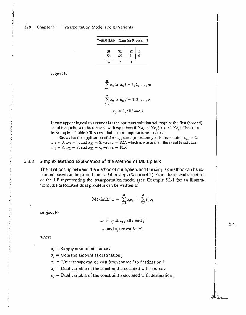
, '220 Chapter 5 Transportation Model and Its Variants
TABLE 5.30 Data for Problem 7
$1$6
2
$1$5
7
$2 5$1 6
1
".'...i:1"
1,1,I
:I;'1
:~!
-1I
subject to
n
2: Xij 2: ai, i = 1, 2, "', mj=1
m
2:x,j ;;::: bj , j = 1,2, ... , ni=1
Xij 2: O,all i and j
It may appear logical to assume that the optimum solution will require the first (second)set of inequalities to be replaced with equations if Lai 2: Lbj (Lai :::;; Lbj ). The counterexample in Table 5.30 shows that this assumption is not correct.
Show that the application of the suggested procedure yields the solution Xu = 2,x12 = 3, X22 = 4, and X23 = 2, with z = $27, which is worse than the feasible solutionXll = 2, Xu = 7, and X23 = 6, with z = $15.
5.3.3 Simplex Method Explanation of the Method of Multipliers
The relationship between the method of multipliers and the simplex method can be explained based on the primal-dual relationships (Section 4.2). From the special structureof the LP representing the transportation model (see Example 5.1-1 for an illustration), the associated dual problem can be written as
m II
Maximize z = 2:ajUj + 2:bjVji=1 j=1
subject to
Ui + Vj S Cij, all i andj
Uj and Vj unrestricted
where
ai == Supply amount at source i
bj = Demand amount at destination j
Gij = Unit transportation cost from source ito destinationj
Ui = Dual variable of the constraint associated with source i
Vj = Dual variable of the constraint associated with destination j
5.4
5.4 The Assignment Model 221
From Formula 2, Section 4.2.4, the objective-function coefficients (reducedcosts) of the variable Xij equal the difference between the left- and right-hand sidesof the corresponding dual constraint-that is, Ui + Vj - Cij' However, we know thatthis quantity must equal zero for each basic variable, which then produces the following result:
Ui + Vj = Cij, for each basic variable Xij'
There are In + n - 1 such equations whose solution (after assuming an arbitq.ryvalue Ul = 0) yields the multipliers Ui and Vj' Once these multipliers are computed, theentering variable is determined from all the nonbasic variables as the one having thelargest positive Ui + Vj - Cij'
The assignment of an arbitrary value to one of the dual variables (i.e., Ul = 0)may appear inconsistent with the way the dual variables are computed using Method 2in Section 4.2.3. Namely, for a given basic solution (and, hence, inverse), the dual valuesmust be unique. Problem 2, Set 5.3c, addresses this point.
PROBLEM SET 5.3C
1. Write the dual problem for the LP of the transportation problem in Example 5.3-5(Table 5.21). Compute the associated optimum dual objective value using the optimaldual values given in Table 5.25, and show that it equals the optimal cost given in theexample.
2. In the transportation model, one of the dual variables assumes an arbitrary value. Thismeans that for the same basic solution, the values of the associated dual variables are notunique. The result appears to contradict the theory of linear programming, where thedual values are determined as the product of the vector of the objective coefficients forthe basic variables and the associated inverse basic matrix (see Method 2, Section 4.2.3).Show that for the transportation model, although the inverse basis is unique, the vectorof basic objective coefficients need not be so. Specifically, show that if Cij is changed tocij + k for all i and j, where k is a constant, then the optimal values of Xij will remain thesame. Hence, the use of an arbitrary value for a dual variable is implicitly equivalent toassuming that a specific constant k is added to all Cij"
5.4 THE ASSIGNMENT MODEL
"The best person for the job" is an apt description of the assignment model. The situation can be illustrated by the assignment of workers with varying degrees of skill tojobs. A job that happens to match a worker's skill costs less than one in which the operator is not as skillful. The objective of the model is to determine the minimum-costassignment of workers to jobs. .
The general assignment model with n workers and n jobs is represented inTable 5.3L
The element Cij represents the cost of assigning worker i to job j (i, j =1, 2, ... , n). There is no loss of generality in assuming that the number of workers always
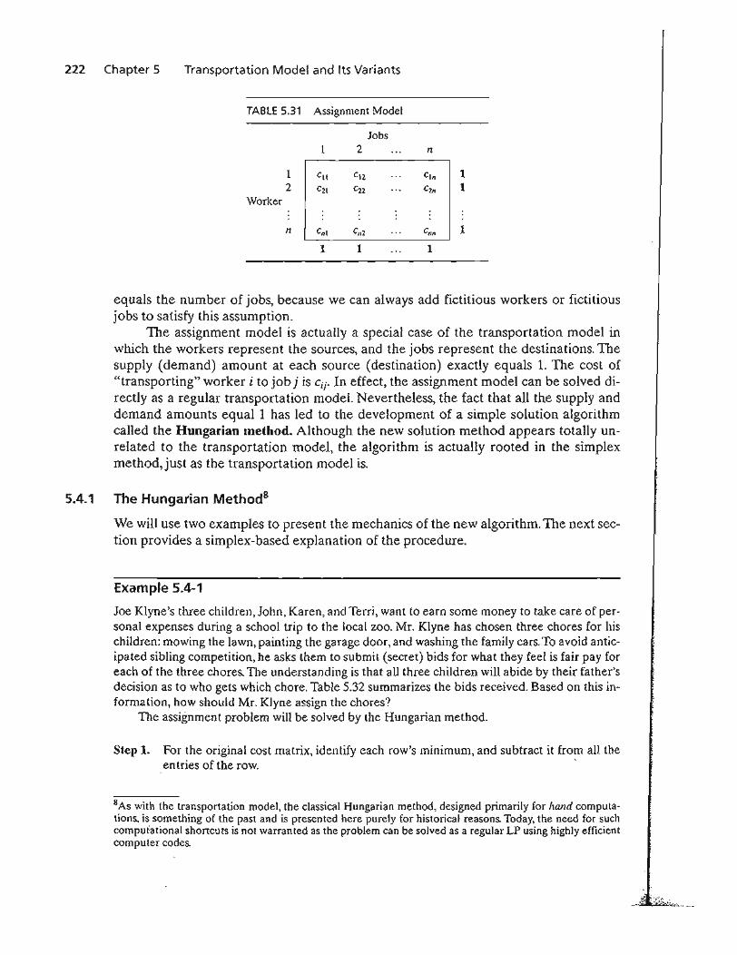
222 Chapter 5 Transportation Model and Its Variants
TABLE 5.31 Assignment Model
Jobs2 n
1 Cll Cl2 Cln 12 C21 C22 cu, 1
Worker
n Cnl '112 Cnn 1
1 1 1
equals the number of jobs, because we can always add fictitious workers or fictitiousjobs to satisfy this assumption.
The assignment model is actually a special case of the transportation model inwhich the workers represent the sources, and the jobs represent the destinations. Thesupply (demand) amount at each source (destination) exactly equals 1. The cost of"transporting" worker i to job j is Cij' In effect, the assignment model can be solved directly as a regular transportation modeL Nevertheless, the fact that all the supply anddemand amounts equal 1 has led to the development of a simple solution algorithmcalled the Hungarian method. Although the new solution method appears totally unrelated to the transportation model, the algorithm is actually rooted in the simplexmethod,just as the transportation model is.
5.4.1 The Hungarian MethodS
We will use two examples to present the mechanics of the new algorithm. The next section provides a simplex-based explanation of the procedure.
Example 5.4-1
Joe Klyne's three children, John, Karen, and Terri, want to earn some money to take care of personal expenses during a school trip to the local zoo. Mr. Klyne has chosen three chores for hischildren: mowing the lawn, painting the garage door, and washing the family cars. To avoid anticipated sibling competition, he asks them to submit (secret) bids for what they feel is fair pay foreach of the three chores. The understanding is that aU three children will abide by their father'sdecision as to who gets which chore. Table 5.32 summarizes the bids received. Based on this information, how should Mr. Klyne assign the chores?
The assignment problem will be solved by the Hungarian method.
Step 1. For the original cost matrix, identify each row's minimum, and subtract it from all theentries of the row. .
8As with the transportation model, the classical Hungarian method, designed primarily for hand computations, is something of the past and is presented here purely for historical reasons. Today, the need for suchcomputational shortcuts is not warranted as the problem can be solved as a regular LP using highly efficientcomputer codes.
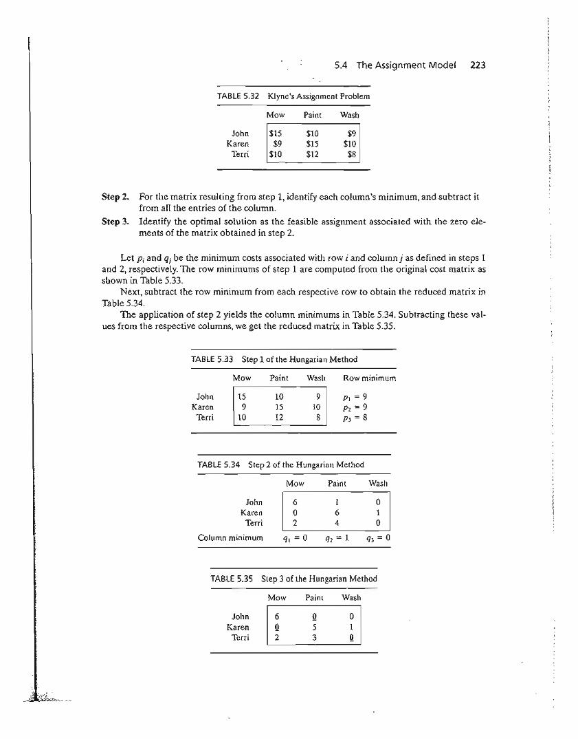
5.4 The Assignment Model 223
TABLE 5.32 Klyne's Assignment Problem
JohnKaren
Terri
Mow
$15$9
$10
Paint
$10$15$12
Wash
$9$10
$8
Step 2. For the matrix resulting from step 1, identify each column's minimum, and subtract itfrom all the entries of the column.
Step 3. Identify the optimal solution as the feasible assignment associated with the zero elements of the matrix obtained in step 2.
Let Pi and qj be the minimum costs associated with row i and column j as defined in steps 1and 2, respectively. The row minimums of step 1 are computed from the original cost matrix asshown in Table 5.33.
Next, subtract the row minimum from each respective row to obtain the reduced matrix inTable 5.34.
The application of step 2 yields the column minimums in Table 5.34. Subtracting these values from the respective columns, we get the reduced matrix in Table 5.35.
TABLE 5.33 Step 1 of the Hungarian Method
JohnKaren
Terri
Mow
159
10
Paint
101512
Wash
9108
Row minimum
PI = 9P2 == 9P3 = 8
TABLE 5.34 Step 2 of the Hungarian Method
Mow Paint Wash
John
I
6 1 0
IKaren 0 6 1
Terri 2 4 0
Column minimum ql = 0 q2 = 1 q3 = 0
TABLE 5.35 Step 3 of the Hungarian Method
Mow Paint Wash
John
I ~D
!IKaren 5
Terri 3
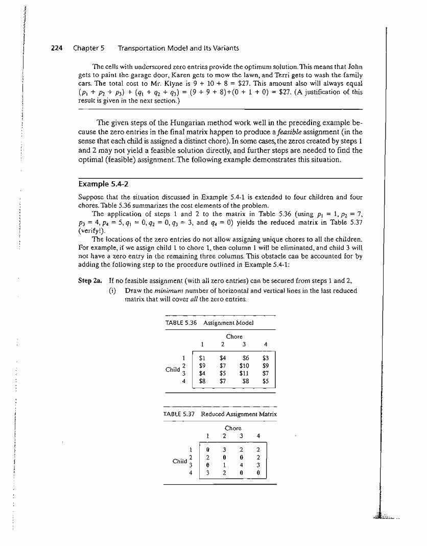
The cells with underscored zero entries provide the optimum solution. This means that Johngets to paint the garage door, Karen gets to mow the lawn, and Terri gets to wash the familycars. The total cost to Mr. Klyne is 9 + 10 + 8 = $27. This amount also will always equal(PI + P2 + P3) + (ql + q2 + q3) = (9 + 9 + 8)+(0 + 1 + 0) = $27. (A justification of thisresult is given in the next section.)
224 Chapter 5 Transportation Model and Its Variants
TIle given steps of the Hungarian method work well in the preceding example because the zero entries in the final matrix happen to produce a feasible assignment (in thesense that each child is assigned a distinct chore). In some cases, the zeros created bysteps 1and 2 may not yield a feasible solution directly, and further steps are needed to find theoptimal (feasible) assignment. The following example demonstrates this situation.
Example 5.4-2
Suppose that the situation discussed in Example 5.4-1 is extended to four children and fourchores. Table 5.36 summarizes the cost elements of the problem.
The application of steps 1 and 2 to the matrix in Table 5.36 (using Pl = 1, P2 = 7,P3 = 4, P4 = 5, ql = 0, q2 = 0, q3 = 3, and q4 = 0) yields the reduced matrix in Table 5.37(verify!).
The locations of the zero entries do not allow assigning unique chores to all the children.For example, if we assign child 1 to chore 1, then column 1 will be eliminated, and child 3 willnot have a zero entry in the remaining three columns. This obstacle can be accounted for byadding the following step to the procedure outlined in Example 5.4-1:
Step 2a. If no feasible assignment (with all zero entries) can be secured from steps 1 and 2,
(i) Draw the minimum number of horizontal and vertical lines in the last reducedmatrix that will cover all the zero entries.
TABLE 5.36 Assignment Model
Chore2 3 4
1 $1 $4 $6 $3
Child ~$9 $7 $10 $9$4 $5 $11 $7
4 $8 $7 $8 $5
TABLE 5.37 Reduced Assignment Matrix
Chore1 2 3 4
1 0 3 2 2
Child;2 0 0 20 1 4 3
4 3 2 0 0
f ....~-.:.... ..•
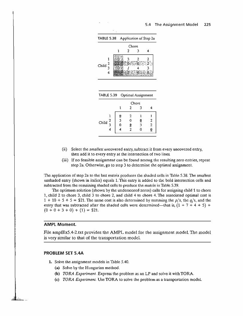
5.4 The Assignment Model 225
TABLE 5.38 Application of Step 2a
1Chore
2 3 4
1
Child ~4
322{J:J)~/i~i;:'~Q';;;{:;::i:';;)
143... .'t. :!~~1~~:1f8t~~hf;ii:;Q~uj
1Y
TABLE 5.39 Optimal Assignment
Chore1 2 3 4
1 !! 2 1 1
Child ~ 3 0 !! 20 !! 3 2
4 4 2 0 !!
(ii) Select the smallest uncovered entry, subtract it from every uncovered entry,then add it to every entry at the intersection of two lines.
(iii) If no feasible assignment can be found among the resulting zero entries, repeatstep 2a. Otherwise, go to step 3 to determine the optimal assignment.
The application of step 2a to the last matrix produces the shaded cells in Table 5.38. The smallestunshaded entry (shown in italics) equals 1. 111is entry is added to the bold intersection cells andsubtracted from the remaining shaded cells to produce the matrix in Table 5.39.
The optimum solution (shown by the underscored zeros) calls for assigning child 1 to chore1, child 2 to chore 3, child 3 to chore 2, and child 4 to chore 4. The associated optimal cost is1 + 10 + 5 + 5 = $21. The same cost is also determined by summing the p/s, the q/s, and theentry that was subtracted after the shaded cells were determined-that is, (1 + 7 + 4 + 5) +(0 + 0 + 3 + 0) + (1) = $21.
AMPL Moment.
File amplEx5.4-2.txt provides the AMPL model for the assignment model. The modelis very similar to that of the transportation model.
PROBLEM SET 5.4A
L Solve the assignment models in Table 5.40.
(a) Solve by the Hungarian method.
(b) TORA Experiment. Express the problem as an LP and solve it with TORA.
(c) TORA Experiment. Use TORA to solve the problem as a transportation model.
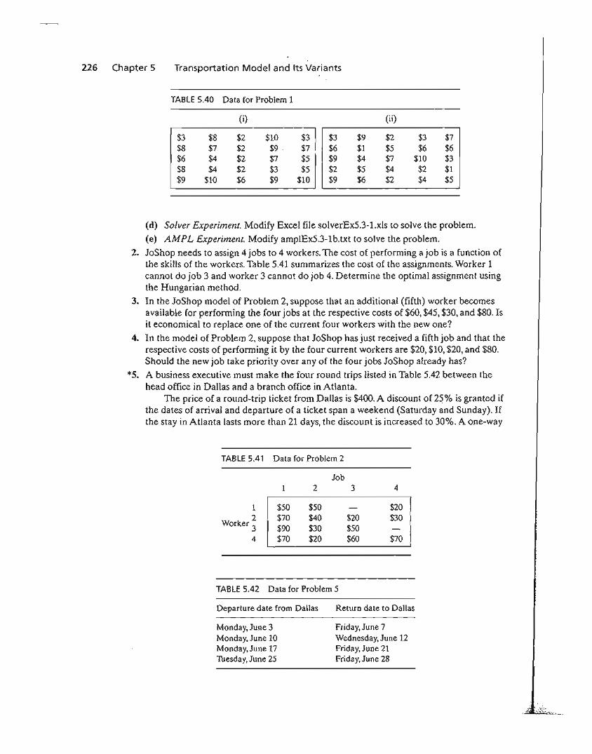
226 Chapter 5 Transportation Model and Its Variants
TABLE 5.40 Data for Problem 1
(0 (ii)
$3 $8 $2 $10 $3 $3 $9 $2 $3 $7$8 $7 $2 $9 . $7 $6 $1 $5 $6 $6$6 $4 $2 $7 $5 $9 $4 $7 $10 $3$8 $4 $2 $3 $5 $2 $5 $4 $2 $1$9 $10 $6 $9 $10 $9 $6 $2 $4 $5
(d) Solver Experiment. Modify Excel file solverEx5.3-l.xls to solve the problem.(e) AMPL Experiment. Modify ampIEx5.3-1b.txt to solve the problem.
2. JoShop needs to assign 4 jobs to 4 workers. The cost of performing a job is a function ofthe skills of the workers. Table 5.41 summarizes the cost of the assignments. Worker 1cannot do job 3 and worker 3 cannot do job 4. Determine the optimal assignment usingthe Hungarian method.
3. In the JoShop model of Problem 2, suppose that an additional (fifth) worker becomesavailable for performing the four jobs at the respective costs of $60, $45, $30, and $80. Isit economical to replace one of the current four workers with the new one?
4. In the model of Problem 2, suppose that JoShop has just received a fifth job and that therespective costs of performing it by the four current workers are $20, $10, $20, and $80.Should the new job take priority over any of the four jobs JoShop already has?
*5. A business executive must make the four round trips listed in Table 5.42 between thehead office in Dallas and a branch office in Atlanta.
The price of a round-trip ticket from Dallas is $400. A discount of 25% is granted ifthe dates of arrival and departure of a ticket span a weekend (Saturday and Sunday). Ifthe stay in Atlanta lasts more than 21 days, the discount is increased to 30%. A one-way
TABLE 5.41 Data for Problem 2
Job2 3 4
1 $50 $50 $202 $70 $40 $20 $30
Worker 3 $90 $30 $504 $70 $20 $60 $70
TABLE 5.42 Data for Problem 5
Departure date from Dallas
Monday, June 3Monday, June 10Monday, June 17Tuesday, June 25
Return date to Dallas
Friday, June 7Wednesday, June 12Friday, June 21Friday, June 28
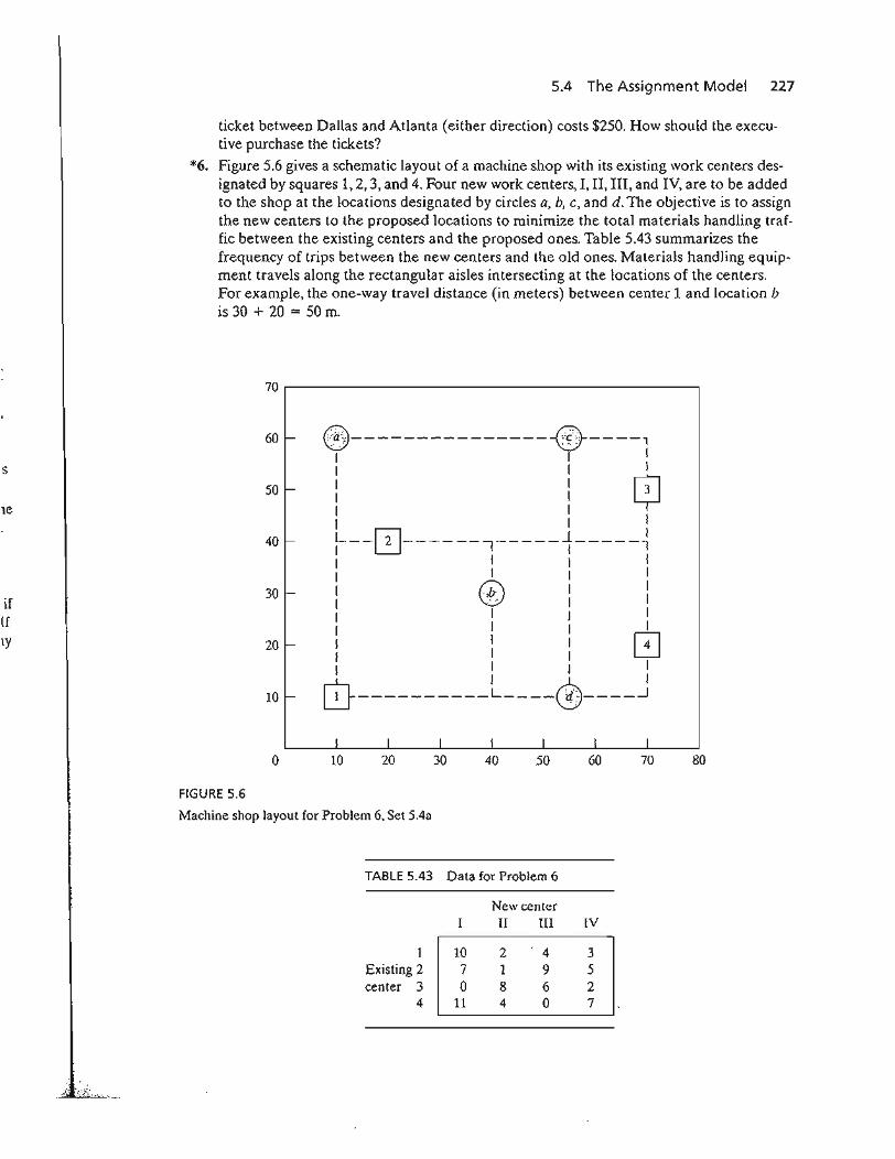
5.4 The Assignment Model 227
ticket between Dallas and Atlanta (either direction) costs $250. How should the executive purchase the tickets?
*6. Figure 5.6 gives a schematic layout of a machine shop with its existing work centers designated by squares 1,2,3, and 4. Four new work centers, I, II, III, and IV, are to be addedto the shop at the locations designated by circles a, b, c, and d. The objective is to assignthe new centers to the proposed locations to minimize the total materials handling traffic between the existing centers and the proposed ones. Table 5.43 summarizes thefrequency of trips between the new centers and the old ones. Materials handling equipment travels along the rectangular aisles intersecting at the locations of the centers.For example, the one-way travel distance (in meters) between center 1 and location bis 30 + 20 "" 50 m.
70 .----------------------------,
s
le
if[fly
60 -
50 -
40 -
30 -
20 -
10-
EV---------------~----,I' 'I: 11 I II I Gl1 I Y1 1 II I I~--[J------I-----1-----l1 I I II 1 I II r];\ I I,1 "..::9 I1 I I I1 J I ,
I I I f4l1 I I L:JI I I I
[!} L QD J
oI
10I
20I
30I
40I
50I
60I
70 80
FIGURE 5.6
Machine shop layout for Problem 6, Set 5.4a
TABLE 5.43 Data for Problem 6
New centerI II III IV
1 10 2 4 3Existing 2 7 1 9 5center 3 0 8 6 2
4 11 4 0 7
228 Chapter 5 Transportation Model and Its Variants
7. In the Industrial Engineering Department at the University of Arkansas, INEG 4904 is acapstone design course intended to allow teams of students to apply the knowledge andskills learned .in the undergraduate curriculum to a practical problem. The members ofeach team select a project manager, identify an appropriate scope for their project, writeand present a proposal, perform necessary tasks for meeting the project objectives, andwrite and present a final report. The course instructor identifies potential projects andprovides appropriate information sheets for each, including contact at the sponsoring organization, project summary, and potential skills needed to complete the project. Eachdesign team is required to submit a report justifying the selection of team members andthe team manager. The report also provides a ranking for each project in order of preference, including justification regarding proper matching of the team's skills with the project objectives. In a specific semester, the following projects were identified: Boeing F-lS,Boeing F-18, Boeing Simulation, Cargil, Cobb-Vantress, ConAgra, Cooper, DaySpring(layout), DaySpring (material handling), IB. Hunt, Raytheon, Tyson South, Tyson East,Wal-Mart, and Yellow Transportation. The projects for Boeing and Raytheon require U.S.citizenship of all team members. Of the eleven design teams available for this semester,four do not meet this requirement.
Devise a procedure for assigning projects to teams and justify the arguments you useto reach a decision.
5.4.2 Simplex Explanation of the Hungarian Method
The assignment problem in which n workers are assigned to n jobs can be representedas an LP model in the following manner: Let eij be the cost of assigning worker i to jobj, and define
if worker i is assigned to job j
otherwise
Then the LP model is given as
n n
Minimize z = L LCijXiji=lj=l
subject ton
2:Xij = l,l = 1,2, ... ,nj=l
n
LXij = 1, j = 1,2, ... , ni=1
x·· = 0 or 1IJ
The optimal solution of the preceding LP model remains unchanged if a constantis added to or subtracted from any row or column of the cost matrix (cij)' To prove thispoint, let Pi and qj be constants subtracted from row i and columnj. Thus, the cost element cij is changed to
5.5
5.5 The Transshipment Model 229
Now
= L LCijXij - constanti j
Because the new objective function differs from the original one by a constant, the optimum values of Xij must be the same in both cases. The development thus shows thatsteps 1 and 2 of the Hungarian method, which call for subtracting Pi from row i andthen subtracting qj from columnj, produce an equivalent assignment model. In this regard, if a feasible solution can be found among the zero entries of the cost matrix created by steps 1 and 2, then it must be optimum because the cost in the modified matrixcannot be less than zero.
If the created zero entries cannot yield a feasible solution (as Example 5.4-2demonstrates), then step 2a (dealing with the covering of the zero entries) must be applied. The validity of this procedure is again rooted in the simplex method of linearprogramming and can be explained by duality theory (Chapter 4) and the complementary slackness theorem (Chapter 7). We will not present the details of the proof herebecause they are somewhat involved.
The reason (PI + P2 + ... + Pn) + (qI + q2 + ... + qn) gives the optimalobjective value is that it represents the dual objective function of the assignmentmodel. This result can be seen through comparison with the dual objective function ofthe transportation model given in Section 5.3.4. [See Bazaraa and Associates (1990, pp.499-508) for the details.]
5.5 THE TRANSSHIPMENT MODEL
The transshipment model recognizes that it may be cheaper to ship through intermediate or transient nodes before reaching the final destination. This concept is more general than that of the regular transportation model, where direct shipments only areallowed between a source and a destination.
This section shows how a transshipment model can be converted to (and solvedas) a regular transportation model using the idea of a buffer.
Example 5.5-1
Two automobile plants, PI and P2, are linked to three dealers, DI, D2, and D3, by way of twotransit centers, T1 and 12, according to the network shown in Figure 5.7. The supply amounts atplants PI and P2 are 1000 and 1200 cars, and the demand amounts at dealers Dl, D2, and D3,are 800, 900, and 500 cars. TIle shipping costs per car (in hundreds of dollars) between pairs ofnodes are shown on the connecting links (or arcs) of the network.
Transshipment occurs in the network in Figure 5.7 because the entire supply amount of2200 (= 1000 + 1200) cars at nodes PI and P2 could conceivably pass through any node of the
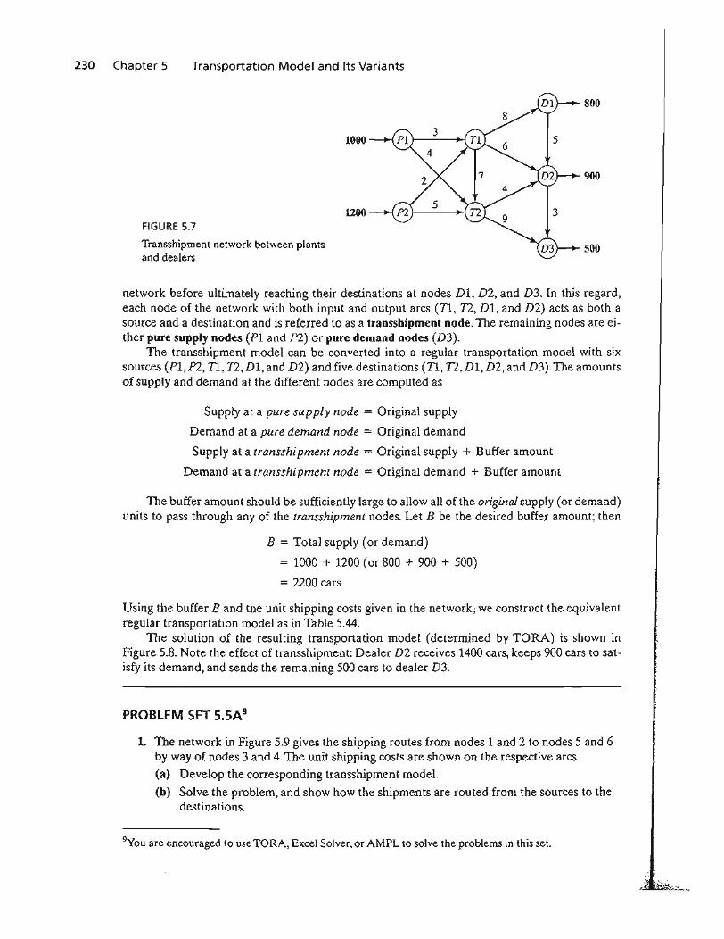
230 Chapter 5 Transportation Model and Its Variants
1000
1200FIGURE 5.7
Transshipment network between plantsand dealers
800
900
500
network before ultimately reaching their destinations at nodes D1, D2, and D3. In this regard,each node of the network with both input and output arcs (11., n, DI, and D2) acts as both asource and a destination and is referred to as a transshipment node. The remaining nodes are either pure supply nodes (PI and Pl) or pure demand nodes (D3).
The transshipment model can be converted into a regular transportation model with sixsources (PI, Pl, 11., n,Dl, and D2) and five destinations (71, n,Dl, D2, and D3).1l1e amountsof supply and demand at the different nodes are computed as
Supply at a pure supply node = Original supply
Demand at a pure demand node = Original demand
Supply at a transshipment node = Original supply + Buffer amount
Demand at a transshipment node = Original demand + Buffer amount
The buffer amount should be sufficiently large to allow all of the original supply (or demand)units to pass through any of the transshipment nodes. Let B be the desired buffer amount; then
B = Total supply (or demand)
= 1000 + 1200 (or 800 + 900 + 500)
= 2200 cars
Using the buffer B and the unit shipping costs given in the network; we construct the equivalentregular transportation model as in Table 5.44.
The solution of the resulting transportation model (determined by TORA) is shown inFigure 5.8. Note the effect of transshipment: Dealer D2 receives 1400 cars, keeps 900 cars to satisfy its demand, and sends the remaining 500 cars to dealer D3.
PROBLEM SET 5.5A9
1. The network in Figure 5.9 gives the shipping routes from nodes 1 and 2 to nodes 5 and 6by way of nodes 3 and 4. The unit shipping costs are shown on the respective arcs.
(a) Develop the corresponding transshipment model.
(b) Solve the problem, and show how the shipments are routed from the sources to thedestinations.
9you are encouraged to use TORA, Excel Solver, or AMPL to solve the problems in this set.
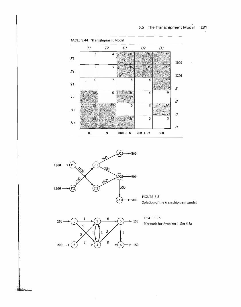
5.5 The Transshipment Model· 231
TABLE 5.44 Transshipment Model
Tl 12 Dl D2 D3
1.,
I{
s
PI
n
n
n
DI
D2o 3
1000
1200
B
B
B
B
B B 800 + B 900 + B 500
150200
800
) 1000
1
900
1200
FIGURE 5.8t 500
Solution of the transshipment model
1
FIGURE 5.9100 150
Network for Problem 1, Set 5.5a
.;.
'; 'X :\~'~"'~!'':'':-._
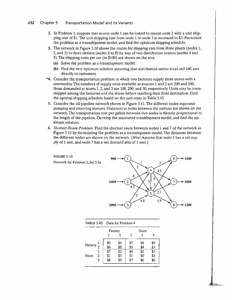
232 Chapter 5 Transportation Model and Its Variants
2. In Problem 1, suppose that source node 1 can be linked to source node 2 with a unit shipping cost of $1. The unit shipping cost from node 1 to node 3 is increased to $5. Formulatethe problem as a transshipment model, and find the optimum shipping schedule.
3. The network in Figure 5.10 shows the routes for shipping cars from three plants (nodes 1,2, and 3) to three dealers (nodes 6 to 8) by way of two distribution centers (nodes 4 and5). The shipping costs per car (in $100) are shown on the arcs.
(a) Solve the problem as a transshipment model.
(b) Find the new optimum solution assuming that distribution center 4 can sell 240 carsdirectly to customers.
*4. Consider the transportation problem in which two factories supply three stores with acommodity. The numbers of supply units available at sources 1 and 2 are 200 and 300;those demanded at stores 1,2, and 3 are 100,200, and 50, respectively. Units may be transshipped among the factories and the stores before reaching their final destination. Findthe optimal shipping schedule based on the unit costs in Table 5.45.
S. Consider the oil pipeline network shown in Figure 5.11. The different nodes representpumping and receiving stations. Distances in miles between the stations are shown on thenetwork. The transportation cost per gallon between two nodes is directly proportional tothe length of the pipeline. Develop the associated transshipment model, and find the optimum solution.
6. Shortest-Route Problem. Find the shortest route between nodes 1 and 7 of the network inFigure 5.12 by formulating the problem as a transshipment model. The distances betweenthe different nodes are shown on the network. (Hint: Assume that node 1 has a net supply of 1 unit, and node 7 has a net demand also of 1 unit.)
FIGURE 5.10
Network for Problem 3, Set 5.5a900
1400
1000
1100
1000
1200
TABLE 5.45 Data for Problem 4
Factory1 2 1
Store2 3
$6 $0] $5 $4 $3-·-S;7-------$2--~··-$-O·------$5-----··$T··
$1 $5 $1 $0 $4$8 $9 $7 $6 $0
1Factory 2
1Store 2
3
$0 $6 $7 $8 $9
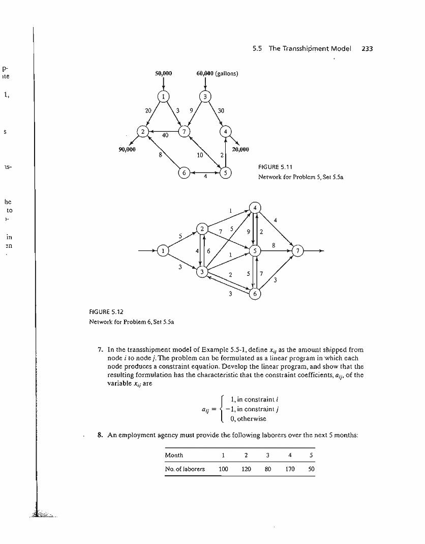
pIte
1,
s
1S-
50,000 60,000 (gallons)
5.5 The Transshipment Model 233
FIGURE 5.11
Network for Problem 5, Set 5.5a
III
~n
FIGURE 5.12
Network for Problem 6, Set 5.5a
7. In the transshipment model of Example 5.5-1, define Xij as the amount shipped fromnode i to node j. The problem can be formulated as a linear program in which eachnode produces a constraint equation. Develop the linear program, and show that theresulting formulation has the characteristic that the constraint coefficients, aij, of thevariable Xij are
{
I, in constraint i
aij = -1, in constraint j
0, otherwise
8. An employment agency must provide the following laborers over the next 5 months:
Month
No. of laborers
1
100
2
120
3
80
4
170
5
50
234 Chapter 5 Transportation Model and Its Variants
Because the cost of labor depends on the length of employment, it may be more economical to keep more laborers than needed during some months of the 5-month planning horizon. The following table estimates the labor cost as a function of the length ofemployment:
Months of employment
Cost per laborer ($)
1
100
2
130
3
180
4
220
5
250
Formulate the problem as a linear program. Then, using proper algebraic manipulations of the constraint equations, show that the model can be converted to a transshipment model, and find the optimum solution. (Hint: Use the transshipment characteristicin Problem 7 to convert the constraints of the scheduling problem into those of the transshipment model.)
REFERENCES
Bazaraa, M., 1. Jarvis, and H. Sherali, Linear Programming and Network Flows, 2nd ed., Wiley,New York, 1990.
Dantzig, G., Linear Programming and Extensions, Princeton University Press, Princeton, N.J.,1963.
Hansen, P. and R. Wendell, "A Note on Airline Commuting," lntelfaces, Vol. 12, No.1, pp. 85-87,1982.
Murty, K., Network Programming, Prentice Hall, Upper Saddle River, NJ, 1992.