Operational Implementation of a Pc Uncertainty Construct

for Conjunction Assessment Risk Analysis

Lauri K. Newman

NASA Goddard Space Flight Center

Matthew D. Hejduk

Astrorum Consulting LLC

Lauren C. Johnson

Omitron Inc.

ABSTRACT

Earlier this year the NASA Conjunction Assessment and Risk Analysis (CARA) project presented the

theoretical and algorithmic aspects of a method to include the uncertainties in the calculation inputs when computing

the probability of collision (Pc) between two space objects, principally uncertainties in the covariances and the hard-

body radius. The output of this calculation approach is to produce rather than a single Pc value an entire probability

density function that will represent the range of possible Pc values given the uncertainties in the inputs and bring CA

risk analysis methodologies more in line with modern risk management theory. The present study provides results

from the exercise of this method against an extended dataset of satellite conjunctions in order to determine the effect

of its use on the evaluation of conjunction assessment (CA) event risk posture. The effects are found to be

considerable: a good number of events are downgraded from or upgraded to a serious risk designation on the basis

of consideration of the Pc uncertainty. The findings counsel the integration of the developed methods into NASA

CA operations.

1. INTRODUCTION

The use of the Probability of Collision (Pc) as the principal metric to assess the likelihood of a collision

between two satellites has become standard practice in the satellite conjunction assessment (CA) and risk analysis

discipline. Previous approaches had focused nearly entirely on the smallest predicted miss distance between the

satellites; but it was recognized that, without including an estimate of the state estimate uncertainties of the two

objects, the significance of the miss distance was difficult to interpret: if the state estimate uncertainties were small,

a quite small miss distance might not be a threatening situation; if the uncertainties were somewhat larger, than a

larger miss distance might actually be more threatening. The calculation and use of the Pc has both remedied this

particular defect of the miss distance and also allowed the CA enterprise to conform more strongly to classical risk

management constructs in that the Pc does give an actual likelihood—a probability—that a collision (or at least a

dangerously close approach) will take place. It has been suggested that CA risk analysis should consider both

likelihood and consequence in forming evaluations, as not all potential collisions are expected to be equally

catastrophic to the protected asset, would generate as much debris, or would threaten through a debris cloud equally

important orbital corridors; and perhaps this is a useful area for expansion for the industry. Yet in comparison to the

relatively primitive method of using miss distance alone, the standardized employment of Pc is a considerable

advance.

Such analyses, however, have been limited to the single calculation of the Pc from the state estimates and

covariances at hand at the time the calculation is performed. The probability of collision calculation, especially in

the nearly ubiquitously-used simplified form that reduces the problem from three to two dimensions, is described in

considerable detail in Chan [1], but a short summary is appropriate here. The two satellites’ states are propagated to

the time of closest approach (TCA), the satellites’ covariance matrices are similarly propagated and combined, a

hard-body radius (HBR) is defined (usually the radius of a supersphere that encapsulates touching circumscribing

spheres about each satellite), the covariance, miss distance, and HBR are projected into the “conjunction plane”

perpendicular to the velocity vector (if a collision is to occur it will take place in that plane), the combined

covariance is placed at the origin in this plane, the HBR is placed one miss distance away at the appropriate angle,

https://ntrs.nasa.gov/search.jsp?R=20160011334 2018-07-07T23:21:23+00:00Z

and the Pc is the portion of the combined covariances’ probability density that falls within the HBR projected

sphere. Researchers have developed transformation methods to accelerate this calculation [1 2], but the basics of the

procedure are extremely similar among the different instantiations; and among these similarities is the fact that none

of them consider the uncertainties in the inputs in order to generate either error statements about the result or a

probability density function (PDF) of Pc possibilities rather than merely a single value. The input covariances,

while expressions of the uncertainties of the propagated states, contain their own uncertainties—both of the orbit

determination (OD) uncertainties at the OD epoch time and additional errors acquired through propagation. The

HBR is often a value that is extremely conservatively sized and, if set to resemble more closely the actual exposed

frontal area expected in the conjunction plane, would require an accompanying error statement. There are yet

additional second-order error sources that should be considered. All of these uncertainties should be characterized

and included in the calculation so that the range of possible values, not just a simple point estimate, can feed the risk

analysis process.

At an engineering conference earlier this year, the NASA Conjunction Assessment Risk Analysis (CARA)

project presented a paper outlining a calculation technique for incorporating these sources of uncertainty into the Pc

calculation [3]. Since that presentation, this functionality has been exercised against an extended set of operational

conjunction assessment data in order to acquire a sense of how the calculations perform, what the PDFs of Pc values

look like and how they compare to the nominal value presently used in operations, and how the use of the PDFs

could modify/enhance operational assessments of risk. This paper will give both an abbreviated review of the

general principles and particular calculation approaches for covariance and HBR error and the results of the above

real-world data exercise of the functionality, the latter to illustrate the operational effect of the presence of risk

assessment data in this form.

2. PROBABILITY UNCERTAINTY AND RISK ASSESSMENT

While there are a number of different methodologies for performing risk assessment, in general the framework

for modern risk management can be traced back to the pioneering work of Kaplan, especially his 1981 article on the

constituent elements of risk [4]. In that work, he identified two such constitutive elements. The first is to

understand risk as a continuous form of a series of “Kaplan Triplets,” in which for a set of possible scenarios the

likelihood and consequence of each scenario’s coming to pass is determined; if one plots these ordered pairs of

likelihood and consequence in a Cartesian system, the result is a “risk curve” that describes the relationship between

these two items. This first element is certainly worthy of extended discussion, especially concerning the details of

its application to CA; but because at its basic level it is well understood by most risk assessment practitioners and

because it is not central to the present study’s purpose, it will not be explained further here. The second constitutive

element, however, is of immediate relevance to the present investigation, and it is this: a likelihood-consequence

relationship, described in an idealized way by a single curve, is in fact not a single curve but an entirely family of

curves (or, said differently, a probability density) that reflect the uncertainties of the inputs in the calculation of

likelihood and consequence. Depending on the confidence level one desires, a number of different individual risk

curves can be constructed; Fig. 1 shows Kaplan’s original illustration of this phenomenon, in which he plots

contours of equal probability.

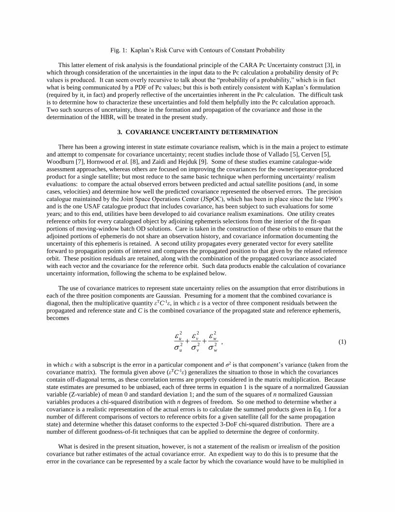
Fig. 1: Kaplan’s Risk Curve with Contours of Constant Probability

This latter element of risk analysis is the foundational principle of the CARA Pc Uncertainty construct [3], in

which through consideration of the uncertainties in the input data to the Pc calculation a probability density of Pc

values is produced. It can seem overly recursive to talk about the “probability of a probability,” which is in fact

what is being communicated by a PDF of Pc values; but this is both entirely consistent with Kaplan’s formulation

(required by it, in fact) and properly reflective of the uncertainties inherent in the Pc calculation. The difficult task

is to determine how to characterize these uncertainties and fold them helpfully into the Pc calculation approach.

Two such sources of uncertainty, those in the formation and propagation of the covariance and those in the

determination of the HBR, will be treated in the present study.

3. COVARIANCE UNCERTAINTY DETERMINATION

There has been a growing interest in state estimate covariance realism, which is in the main a project to estimate

and attempt to compensate for covariance uncertainty; recent studies include those of Vallado [5], Cerven [5],

Woodburn [7], Hornwood et al. [8], and Zaidi and Hejduk [9]. Some of these studies examine catalogue-wide

assessment approaches, whereas others are focused on improving the covariances for the owner/operator-produced

product for a single satellite; but most reduce to the same basic technique when performing uncertainty/ realism

evaluations: to compare the actual observed errors between predicted and actual satellite positions (and, in some

cases, velocities) and determine how well the predicted covariance represented the observed errors. The precision

catalogue maintained by the Joint Space Operations Center (JSpOC), which has been in place since the late 1990’s

and is the one USAF catalogue product that includes covariance, has been subject to such evaluations for some

years; and to this end, utilities have been developed to aid covariance realism examinations. One utility creates

reference orbits for every catalogued object by adjoining ephemeris selections from the interior of the fit-span

portions of moving-window batch OD solutions. Care is taken in the construction of these orbits to ensure that the

adjoined portions of ephemeris do not share an observation history, and covariance information documenting the

uncertainty of this ephemeris is retained. A second utility propagates every generated vector for every satellite

forward to propagation points of interest and compares the propagated position to that given by the related reference

orbit. These position residuals are retained, along with the combination of the propagated covariance associated

with each vector and the covariance for the reference orbit. Such data products enable the calculation of covariance

uncertainty information, following the schema to be explained below.

The use of covariance matrices to represent state uncertainty relies on the assumption that error distributions in

each of the three position components are Gaussian. Presuming for a moment that the combined covariance is

diagonal, then the multiplicative quantity εTC-1ε, in which ε is a vector of three component residuals between the

propagated and reference state and C is the combined covariance of the propagated state and reference ephemeris,

becomes

2

2

2

2

2

2

w

w

v

v

u

u

,

(1)

in which ε with a subscript is the error in a particular component and σ2 is that component’s variance (taken from the

covariance matrix). The formula given above (εTC-1ε) generalizes the situation to those in which the covariances

contain off-diagonal terms, as these correlation terms are properly considered in the matrix multiplication. Because

state estimates are presumed to be unbiased, each of three terms in equation 1 is the square of a normalized Gaussian

variable (Z-variable) of mean 0 and standard deviation 1; and the sum of the squares of n normalized Gaussian

variables produces a chi-squared distribution with n degrees of freedom. So one method to determine whether a

covariance is a realistic representation of the actual errors is to calculate the summed products given in Eq. 1 for a

number of different comparisons of vectors to reference orbits for a given satellite (all for the same propagation

state) and determine whether this dataset conforms to the expected 3-DoF chi-squared distribution. There are a

number of different goodness-of-fit techniques that can be applied to determine the degree of conformity.

What is desired in the present situation, however, is not a statement of the realism or irrealism of the position

covariance but rather estimates of the actual covariance error. An expedient way to do this is to presume that the

error in the covariance can be represented by a scale factor by which the covariance would have to be multiplied in

order to make it representative. There are, of course, more complex ways to represent and/or remediate position

covariance error, such as maintaining a separate scale factor for each axis and an angle through which the primary

axis of the covariance must be rotated in order to make it perfectly representative; but in considering the more

modest needs of the present application and the potential aliasing among multiple variables in a covariance realism

solution, a single scale factor paradigm is quite serviceable. The expected value of an n-DoF chi-squared

distribution is n; so one approach to generating a set of scale factors is to calculate for every set of evaluated

residuals the scale factor that would need to be applied to force the εTC-1ε value to 3 (since one is expecting a 3-DoF

chi-squared distribution); this would produce a set of scale factors whose PDF could be said to characterize the

expected covariance errors. While this approach begins to approach the mark, it falls short in that it is trying to

force every covariance evaluation to produce the expected value; in no distribution except for the uniform

distribution is it imposed that every data point assume the value of the mean (the expected value), and certainly not

with the chi-squared distribution. A minor repair that rectifies this situation is very easy to implement: one

generates a set of chi-squared calculations (99 such calculations for the sake of this explanation), rank-orders these

calculations, and aligns these with the first through 99th percentiles of the 3-DoF chi-squared distribution. The scale

factors to be calculated are thus not the value to force each chi-square calculation to the value of 3 but rather what is

needed at each percentile level to make the calculation equal the chi-squared distribution value for that level. It is

this set of scale factors that can serve as a reasonable estimate of covariance error in that it is the application of this

disparate set of scale factors that would result in producing the hypothesized distribution of normalized residuals.

Fig. 2 below shows for a set of covariance evaluations for a single satellite the empirical distribution of chi-squared

variables, the theoretical distribution to which they should conform, and the distribution of scale factors needed to

make the empirical distribution match the theoretical one.

Fig. 2: Empirical, Theoretical, and Scale Factor Distributions for a Single Satellite

It is important to point out how this approach differs from other techniques presently employed that explore Pc

sensitivity to covariance size through manipulation of the primary and secondary covariance [10]. Typically, these

techniques either scale the combined covariance in the conjunction plane by a uniformly-spaced set of scale factors,

or they scale the primary and secondary covariances separately, perhaps using different scale factor sets. In either

case, the result is a set of Pc values calculated from all combinations of the two different covariance scalings; and

the highest Pc value is taken as the worst case that could arise if there is uncertainty in the covariance.

If pursued in the extreme, i.e., with very large spans of possible scale factors, such a technique approaches the

“maximum Pc” calculation techniques documented in the literature [11]; and the emergent maximum Pc is no longer

a probability at all: it is a statement of the worst that could be produced if a number of particular conditions inhere,

but there is no estimate of the likelihood that such conditions will in fact arise for the case under investigataion; so

the number is not easily used in a risk assessment context. The approach used in the present study is different

because the PDF of possible scale factors includes by its very nature the likelihood that each scale factor will arise

(recall that each is paired with the matching percentile point of the chi-squared distribution); so a set of Monte Carlo

trials that draw from such PDFs will yield a set of Pc values that, if examined by percentile, will possess the

likelihood defined by that particular percentile level. Uniform scaling within bounded scale factor ranges, however,

can avoid the “PcMax” phenomenon and serve as a reasonable method to ferret out dangerous conjunctions that

could in fact arise given expected errors in the covariances.

4. ANALYSIS DATASET AND EXPERIMENT METHODOLOGY

To examine the practical effect of employing this method of characterizing covariance uncertainty in a CA

context, the following dataset and computational methods were deployed. About fourteen months’ worth of

conjunction data on two primary satellites was selected for post-processing analysis. The two satellites are the

NASA Earth-observation satellites Aqua and Aura; both of these occupy near-circular, sun-synchronous orbits

slightly above 700 km—a congested region that presently houses many payloads, is subject to a good bit of the

debris from the Fengyun-1C and Iridium-COSMOS breakups, and tends to generate a large number of conjunctions.

The dataset runs from 1 MAY 2015 to 30 JUN 2016; the JSpOC precision orbit maintenance system conducted their

last service release at the beginning of May 2015 (which included significant covariance accuracy improvements),

so this data span is about the longest period possible that incorporates these JSpOC software enhancements. Slightly

more than 9,000 conjunctions were examined.

While this dataset includes a significant number of conjunctions over all Pc values, it is often useful in the

analysis of such data to divide the dataset broadly by severity in order both to make the results more easily

assimilatable and to determine whether different severity categories exhibit correspondingly different behavior. In

CARA operations, conjunctions are divided by Pc level into three color groups, each of which has different

operational implications. Green events are those with a Pc level less than 1E-07; such events are of a low enough

likelihood not to require any immediate additional monitoring or attention. Red events are those with a Pc level

greater than a value in the neighborhood of 1E-04 (values between 1E-04 and ~5E-04 can be employed for this

threshold; for the present analysis, a value of 1E-04 is used for simplicity). These events are considered quite

serious operationally; they engender specialized analysis, extensive briefings to the satellite owner/operator, and

often maneuver planning and execution support. Events with Pc values falling between these two thresholds are

assigned a yellow color; such events do not demand high-interest-event processing when received, but they well

could increase in severity and become truly threatening; so they are given a heightened monitoring profile, which

often includes manual examination of the secondary object’s OD and, if warranted, requests for increased sensor

tasking. It should be mentioned that any given conjunction event typically produces multiple re-assessments of the

severity as new tracking is received on both objects; it is common to receive three separate updates per day for each

conjunction, and sometimes more if the conjunction is serious and merits manual examination at the JSpOC. An

event can thus assume different colors throughout its life cycle, with the current color level determined by the most

recent update. The data tabulations to follow treat each update as an individual statement of risk to be evaluated,

even though an entire group of such updates might arise from a single conjunction event.

It is also important when examining Pc error or trending behavior to consider the time to TCA. Updates six

days from TCA, for which propagation times to TCA are longest and thus where uncertainties are greatest, can

exhibit quite different behavior from updates close to TCA, which require only short propagation times. Within

each color band, results in the following section are further segregated by time to TCA.

For each update, the experiment was performed as follows. Using covariance evaluation data (as described in

the previous section) for all secondary objects encountered in the CA data set (May 2015 to June 2016), sets of scale

factors were generated for all primary and secondary objects in the dataset. For each conjunction report, ten

thousand scale factor samples (with replacement) were drawn from the primary and the secondary scale factor

datasets, producing ten thousand ordered pairs of scale factors. The scale factors in each such ordered pair were

applied to the primary and secondary covariances, respectively, and the Pc calculated; this produced ten thousand Pc

calculations for each event update. Each set of Pc data was then summarized by percentile levels and presented for

analysis.

5. EFFECT OF COVARIANCE UNCERTAINTY ON EVENTS

Spread of Covariance PDF Results

Before trying to extract operational implications or significance from considering covariance uncertainty, it is

necessary to perform some exploratory analysis in order to understand the basic characteristics of this new data type;

and the first such examination is of the actual span of the resultant Pc PDF. One is curious whether the spans are

relatively narrow (perhaps less than an order of magnitude [OoM]) or are in general quite broad. If they are narrow,

then one might be able to work with either the median value or an upper-percentile value (perhaps the 95th

percentile) as a reasonable single-point representation of the entire PDF; if they are broad, it will be necessary to

consider multiple percentile points. It is also of interest whether large overall differences in span are observed

between the different event color divisions and as a function of time to TCA.

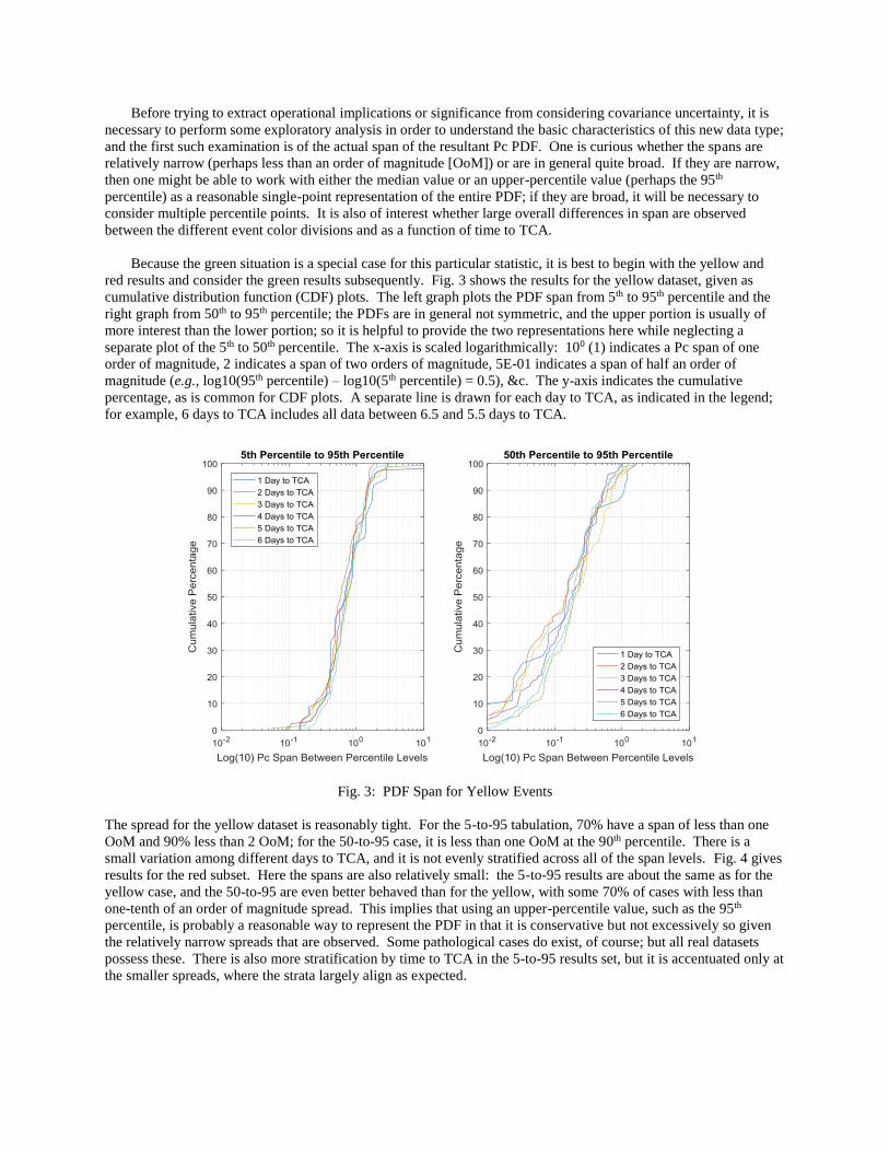
Because the green situation is a special case for this particular statistic, it is best to begin with the yellow and

red results and consider the green results subsequently. Fig. 3 shows the results for the yellow dataset, given as

cumulative distribution function (CDF) plots. The left graph plots the PDF span from 5th to 95th percentile and the

right graph from 50th to 95th percentile; the PDFs are in general not symmetric, and the upper portion is usually of

more interest than the lower portion; so it is helpful to provide the two representations here while neglecting a

separate plot of the 5th to 50th percentile. The x-axis is scaled logarithmically: 100 (1) indicates a Pc span of one

order of magnitude, 2 indicates a span of two orders of magnitude, 5E-01 indicates a span of half an order of

magnitude (e.g., log10(95th percentile) – log10(5th percentile) = 0.5), &c. The y-axis indicates the cumulative

percentage, as is common for CDF plots. A separate line is drawn for each day to TCA, as indicated in the legend;

for example, 6 days to TCA includes all data between 6.5 and 5.5 days to TCA.

Fig. 3: PDF Span for Yellow Events

The spread for the yellow dataset is reasonably tight. For the 5-to-95 tabulation, 70% have a span of less than one

OoM and 90% less than 2 OoM; for the 50-to-95 case, it is less than one OoM at the 90th percentile. There is a

small variation among different days to TCA, and it is not evenly stratified across all of the span levels. Fig. 4 gives

results for the red subset. Here the spans are also relatively small: the 5-to-95 results are about the same as for the

yellow case, and the 50-to-95 are even better behaved than for the yellow, with some 70% of cases with less than

one-tenth of an order of magnitude spread. This implies that using an upper-percentile value, such as the 95th

percentile, is probably a reasonable way to represent the PDF in that it is conservative but not excessively so given

the relatively narrow spreads that are observed. Some pathological cases do exist, of course; but all real datasets

possess these. There is also more stratification by time to TCA in the 5-to-95 results set, but it is accentuated only at

the smaller spreads, where the strata largely align as expected.

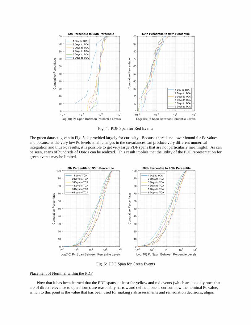
Fig. 4: PDF Span for Red Events

The green dataset, given in Fig. 5, is provided largely for curiosity. Because there is no lower bound for Pc values

and because at the very low Pc levels small changes in the covariances can produce very different numerical

integration and thus Pc results, it is possible to get very large PDF spans that are not particularly meaningful. As can

be seen, spans of hundreds of OoMs can be realized. This result implies that the utility of the PDF representation for

green events may be limited.

Fig. 5: PDF Span for Green Events

Placement of Nominal within the PDF

Now that it has been learned that the PDF spans, at least for yellow and red events (which are the only ones that

are of direct relevance to operations), are reasonably narrow and defined, one is curious how the nominal Pc value,

which to this point is the value that has been used for making risk assessments and remediation decisions, aligns

within the PDF. The diagram given in Fig. 6 below represents this issue graphically: the Pc PDF created by

employing the scale factor set is divided into percentile bins, and one is interested in the particular bin into which the

nominal Pc value for that event falls. In Fig. 6, it happens to be in the 32-50th percentile bin. What is of interest

here is whether the incorporation of covariance uncertainty tends overall to increase the Pc, decrease the Pc, or leave

it at more or less the same level as the nominal.

Fig. 6: Relationship of Nominal Value to PDF

This alignment is determined for all of the updates in the dataset and the results provided in the bar graphs that

follow. Fig. 7 shows the results for the green dataset, which as stated previously are of perhaps the least operational

relevance. It is interesting, however, that in the great majority of cases the nominal value lies below the entire

tabulated PDF. As the time to TCA is reduced, there is more overlap between the nominal and the PDF, but even

then only some 30% of the cases at one day to TCA overlap with the tabulated PDF.

1 %2.5 %5 %

95 %97.5 %99 %

25 %

32 %

68 %

75 %

50 %

Nominal

PDF

Fig. 7: Placement of Nominal Pc Value within Pc PDF; Green Events

The situation for the yellow dataset is given in Fig. 8. Here one encounters a much different situation, and one

that seems to be bimodal or bifurcated. About 25% of events have their nominal entirely below the yellow PDF and

over 50% below the 5% point; this indicates that the actual Pc is somewhat higher than the nominal would indicate

for a considerable number of yellow events. However, a different 30% place the nominal at the 95 th percentile or

higher, and this percentage increase to almost 40% at one day to TCA; so there is also a large number of events

whose actual Pc is probably lower than the nominal value would indicate. Less than one-third of events fall between

the 5th and 95th percentile, indicating that the consideration of covariance uncertainty is potentially significant: it

does not in the main simply reproduce the nominal value but pushes to both lower and higher extremes.

Fig. 8: Placement of Nominal Pc Value within Pc PDF; Yellow Events

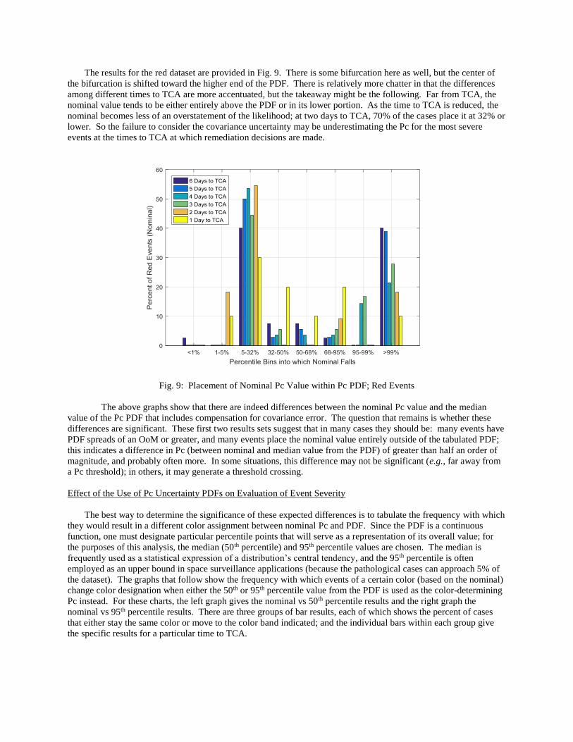
The results for the red dataset are provided in Fig. 9. There is some bifurcation here as well, but the center of

the bifurcation is shifted toward the higher end of the PDF. There is relatively more chatter in that the differences

among different times to TCA are more accentuated, but the takeaway might be the following. Far from TCA, the

nominal value tends to be either entirely above the PDF or in its lower portion. As the time to TCA is reduced, the

nominal becomes less of an overstatement of the likelihood; at two days to TCA, 70% of the cases place it at 32% or

lower. So the failure to consider the covariance uncertainty may be underestimating the Pc for the most severe

events at the times to TCA at which remediation decisions are made.

Fig. 9: Placement of Nominal Pc Value within Pc PDF; Red Events

The above graphs show that there are indeed differences between the nominal Pc value and the median

value of the Pc PDF that includes compensation for covariance error. The question that remains is whether these

differences are significant. These first two results sets suggest that in many cases they should be: many events have

PDF spreads of an OoM or greater, and many events place the nominal value entirely outside of the tabulated PDF;

this indicates a difference in Pc (between nominal and median value from the PDF) of greater than half an order of

magnitude, and probably often more. In some situations, this difference may not be significant (e.g., far away from

a Pc threshold); in others, it may generate a threshold crossing.

Effect of the Use of Pc Uncertainty PDFs on Evaluation of Event Severity

The best way to determine the significance of these expected differences is to tabulate the frequency with which

they would result in a different color assignment between nominal Pc and PDF. Since the PDF is a continuous

function, one must designate particular percentile points that will serve as a representation of its overall value; for

the purposes of this analysis, the median (50th percentile) and 95th percentile values are chosen. The median is

frequently used as a statistical expression of a distribution’s central tendency, and the 95th percentile is often

employed as an upper bound in space surveillance applications (because the pathological cases can approach 5% of

the dataset). The graphs that follow show the frequency with which events of a certain color (based on the nominal)

change color designation when either the 50th or 95th percentile value from the PDF is used as the color-determining

Pc instead. For these charts, the left graph gives the nominal vs 50th percentile results and the right graph the

nominal vs 95th percentile results. There are three groups of bar results, each of which shows the percent of cases

that either stay the same color or move to the color band indicated; and the individual bars within each group give

the specific results for a particular time to TCA.

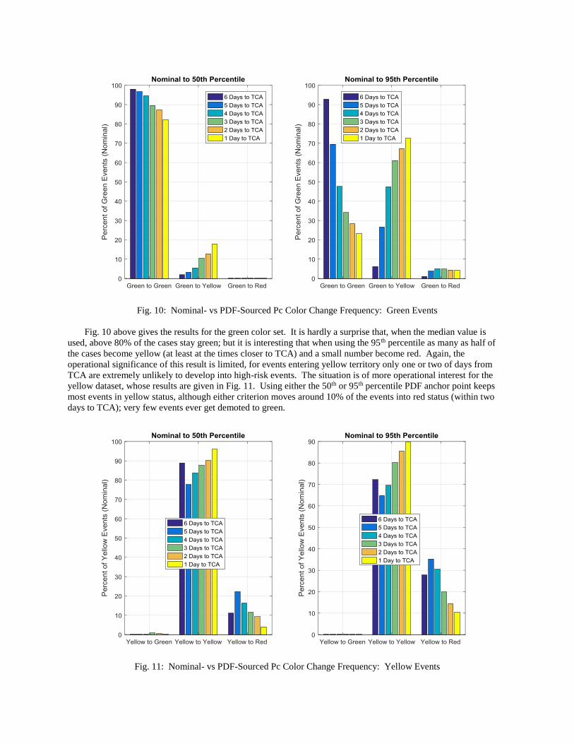
Fig. 10: Nominal- vs PDF-Sourced Pc Color Change Frequency: Green Events

Fig. 10 above gives the results for the green color set. It is hardly a surprise that, when the median value is

used, above 80% of the cases stay green; but it is interesting that when using the 95th percentile as many as half of

the cases become yellow (at least at the times closer to TCA) and a small number become red. Again, the

operational significance of this result is limited, for events entering yellow territory only one or two of days from

TCA are extremely unlikely to develop into high-risk events. The situation is of more operational interest for the

yellow dataset, whose results are given in Fig. 11. Using either the 50th or 95th percentile PDF anchor point keeps

most events in yellow status, although either criterion moves around 10% of the events into red status (within two

days to TCA); very few events ever get demoted to green.

Fig. 11: Nominal- vs PDF-Sourced Pc Color Change Frequency: Yellow Events

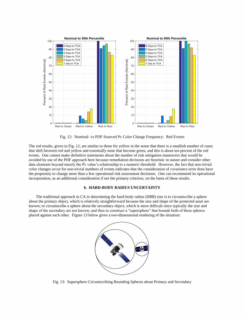
Fig. 12: Nominal- vs PDF-Sourced Pc Color Change Frequency: Red Events

The red results, given in Fig. 12, are similar to those for yellow in the sense that there is a smallish number of cases

that shift between red and yellow and essentially none that become green, and this is about ten percent of the red

events. One cannot make definitive statements about the number of risk mitigation maneuvers that would be

avoided by use of the PDF approach here because remediation decisions are heuristic in nature and consider other

data elements beyond merely the Pc value’s relationship to a numeric threshold. However, the fact that non-trivial

color changes occur for non-trivial numbers of events indicates that the consideration of covariance error does have

the propensity to change more than a few operational risk assessment decisions. One can recommend its operational

incorporation, as an additional consideration if not the primary criterion, on the basis of these results.

6. HARD-BODY RADIUS UNCERTAINTY

The traditional approach in CA to determining the hard-body radius (HBR) size is to circumscribe a sphere

about the primary object, which is relatively straightforward because the size and shape of the protected asset are

known; to circumscribe a sphere about the secondary object, which is more difficult since typically the size and

shape of the secondary are not known; and then to construct a “supersphere” that bounds both of these spheres

placed against each other. Figure 13 below gives a two-dimensional rendering of the situation:

Fig. 13: Supersphere Circumscribing Bounding Spheres about Primary and Secondary

One can see even from this merely notional rendering that there is a fair amount of “white space” within each

bounding sphere. Focusing on the primary object for the moment, if a small secondary object were to penetrate the

bounding sphere of the primary, there is a greater than even chance that it would miss the primary satellite entirely.

In cases in which such satellites are asymmetrically shaped and have large appendages, the bounding sphere can be

an even greater overstatement of the satellite’s actual vulnerable surface.

If the steering law of the primary satellite is known, it is then possible to determine the satellite’s actual

projected are in the conjunction plane for a particular event; in such a case, a contour integral about the projected

area (with this area uniformly grown in each of the two planar dimensions to account for the expected size of the

secondary object) constitutes the most accurate integration technique for computing the two-dimensional Pc. If such

information is not available, then a probabilistic technique can be used to provide a range of Pc values that are more

realistic than those obtained with the circumscribing sphere approach. First, one constructs a moderate-fidelity CAD

model of the satellite; an acceptable level of fidelity for such a model is to restrict oneself to rectangular prisms,

cylinders, and spheres. Next, one rotates this satellite through all possible orientations and projects each orientation

into a fixed plane. Finally, one calculates the area of each planar projection, using a Monte Carlo area calculation or

similar technique; one can represent these values as actual areas or determine the equivalent circular area of each

and thus the equivalent circular area radius. A PDF of either quantity can then be used to determine a corresponding

set of Pc values. This PDF should, of course, have a median value that is considerably smaller than the nominal

value calculated with the usual circumscribing sphere technique, and even the upper-percentile points should be

notably smaller as well for most satellite types.

7. PRACTICAL EFFECT OF CONSIDERING HBR UNCERTAINTY

To characterize the practical effect of using this projected area technique as a basis for the HBR, the following

dataset was analyzed. Data from the same period as described in Section IV above were used, but the Hubble Space

Telescope and the GRACE 1 and 2 satellites were examined, as the project possessed high-fidelity dimensions sets

for these satellites, facilitating CAD model construction. The experiment involving CAD model construction,

rotation, planar projection, and area tabulation was performed for these satellites and HBR PDFs thus obtained. All

of the conjunctions in the dataset were reprocessed using the 50th and 95th percentile HBR levels to generate new Pc

values, which were then compared to the nominal Pc values.

Fig 14: Relationship between Nominal Pc and Pc Calculated from HBR PDF

So long as the HBR remain significantly smaller than the miss distance and covariance sizes, the calculated 2-D

Pc follows a proportional relationship to the integration area described by the HBR. The Pc offset between two

different HBR values can either be calculated explicitly or, if more convenient, derived directly from experimental

data. The chart in Fig. 14 provides the offsets between the standard HBR values used in CARA operations for the

HST and GRACE satellites (10m for the former and 20m for the latter) and what is calculated when the 50th and 95th

percentile value from the full set of satellite projected areas is employed.

For HST, a little more than an OoM’s difference is observed between the nominal and the 95th percentile, and for

GRACE around three OoMs. The HBR span is rather tight in that the offset is somewhat less when using only the

50th percentile, but not significantly so; the principal portion of the Pc reduction is due simply to the significant

oversizing typically realized by using the circumscribing sphere method of HBR determination. The 99th percentile

lines are not shown on this graph because they are not visually distinguishable from the 95th percentile. From this, a

recommendation for operational implementation may be simply to use the largest projected area that the primary

satellite presents in any potential orientation; the differences between doing this and taking percentile points from a

full rotation experiment are not that great, and this “worst case” approach for primary sizing eliminates

disagreements about which percentile point to use or whether this probabilistic method is unacceptably risky. One

can add a small addition to the HBR value to account for the secondary sizing, as discussed in the previous CARA

paper on this subject [3].

Finally, it is of some interest how many red and yellow events from the dataset would have been assigned a

different color based on percentile points from the HBR PDF results as opposed to the nominal Pc. The table below

shows this change history for the dataset described at the beginning of this section.

Table 1: % of Yellow and Red Events with Color Changed by Use of HBR PDF

Yellow to Green Red to Yellow

50th Percentile Projected Area 41.1% of Yellow Events 100% of Red Events

95th Percentile Projected Area 35.1% of Yellow Events 91.2% of Red Events

These results are not insignificant: if one accepts the operational recommendation stated above and thus opts to use

something at or close to the 95th percentile, one might expect the dismissal of the great majority of red events for the

two satellites studied and a less striking but still notable reduction in the number of yellow events that will require

heightened monitoring. Such a reduction is substantial enough to advance itself as a suitable candidate for

operational implementation. In fairness, if the HBR settings used operationally had been set much more closely to

the actual circumscribing sphere sizes for the primaries (HBR size is at the choice of the particular owner/operator,

and some like to use larger sizes for additional conservatism), the differences between the two approaches would not

have been so great. But if an HBR setting is to be changed operationally, usually a compelling reason is necessary

for the modification; so the present analysis can, at the least, counsel an HBR setting much closer to the primary’s

actual circumscribing sphere size, even if there is some resistance to using an HBR value that produces an

equivalent area to the satellite’s maximum planar projected area.

8. CONCLUSIONS

Both the covariance and HBR uncertainty paradigms, laid out in an earlier conference paper [3], do seem

appropriately behaved and properly suited to influence CA operations. The covariance uncertainty is perhaps the

more compelling of the two as a construct in that in some situations it will reduce the Pc and in others in will

increase it, and in some cases these changes are substantial and affect very much the overall risk posture of the

event. The HBR uncertainty behaves more like a bias offset, as the actual PDF of HBR sizes is relatively tight

(meaning that most of the modification in the Pc value is wrought by the simple movement to a true projected area

paradigm). It is seen as operationally helpful to bring adjustments in both areas to the risk assessment situation, as

both have the ability to impose significant changes on the Pc. Keeping the effects broken out separately is a helpful

way to allow modifications to be traced back to their source, as shown in the sample operational plot given in Fig.

15. In this representation, a nested Monte Carlo is used to generate the PDF for the total effect.

Fig 15: Sample Operational Plot showing PDFs in Covariance, HBR, and Combined Effect

9. REFERENCES

[1] Chan, F.C. Spacecraft Collision Probability. El Segundo, CA: The Aerospace Press, 2008.

[2] Alfano, S. “A Numerical Implementation of Spherical Object Collision Probability.” Journal of the

Astronautical Sciences Vol. 63, No. 1 (January-March 2005), pp. 103-109.

[3] Hejduk, M.D. and Johnson, L.C. “Approaches to Evaluating Probability of Collision Uncertainty.” 2015

AAS/AIAA Space Flight Mechanics Meeting, Napa CA, February 2015.

[4] Kaplan, S. and Garrick, B. “On the Quantitative Definition of Risk.” Risk Analysis, Vol. 1 No. 1, pp. 11-27.

[5] Vallado, D.A. and Seago, J.H. “Covariance Realism.” AAS Astrodynamics Specialists Conference (paper #09-

304), Pittsburg PA, August 2009.

[6] Cerven, W.T. “Covariance Error Assessment, Correction, and Impact on Probability of Collision.” 21st

AAS/AIAA Space Flight Mechanics Meeting, New Orleans, LA, January 2011.

[7] Woodburn, J. and Tanygin, S. “Coordinate Effects on the Use of Orbit Error Uncertainty.” International

Symposium on Space Flight Dynamics, Laurel MD, May 2014.

[8] Hornwood, J.T. et al. “Beyond Covariance Realism: a New Metric for Uncertainty Realism.” SPIE

Proceedings: Signal and Data Processing of Small Targets 2014, vol. 9092, 2014.

[9] Zaidi, W.H. and Hejduk, M.D. “Earth Observing System Covariance Realism. AAS/AIAA Astrodynamics

Specialists Conference, Long Beach CA, September 2016.

[10] Laporte, F. “JAC Software, Solving Conjunction Assessment Issues.” 2014 AMOS Technical Conference,

Maui HI, Septermber 2014.