Embed Size (px)
Citation preview

Technische Universität München
FORSCHUNGSPRAKTIKUM
Implementation of an uncertainty quantification tool in MATLAB
Author:
Matic Češnovar
Registration Number:
03633800
Supervisor:
Prof. Wolfgang Polifke, Ph.D.
M.Sc. Alexander Avdonin
24th of November, 2016
Professur für Thermofluiddynamik
Prof. Wolfgang Polifke, Ph.D.


Erklärung:
Hiermit versichere ich, die vorliegende Arbeit selbstständig verfasst zu haben. Ich habe keine anderen Quellen und Hilfsmittel als die angegebenen verwendet.
München, 24.11.2016
Matic Češnovar
________________


Abstract
The present work is dedicated to implement an uncertainty quantification tool in MATLAB using
the non-intrusive polynomial chaos expansion method and to examine the tool performance
with an application test case. Given uniformly or normally distributed uncertain parameters, the
tool computes the output quantities of interest. The test case is based on data of a recent
scientific paper in the field of uncertainty quantification of thermoacoustic instabilities. The tool
results for analytic moments of the uncertain quantities were compared to the results from the
paper, where authors were using adjoints and Monte Carlo simulation. It was shown that the
outputs of both methods are very comparable, the higher the order - the lower the difference,
while the computation time was reduced. The tool results for local sensitivities were verified
using the finite difference method. The results were still comparable, however, it was found
that increase in polynomial chaos expansion order could lead to higher local fluctuations of the
response function (approximation). The reduction of computation time and reliable results
show, that the tool can be used instead of Monte Carlos simulation for small numbers of input
parameters. Furthermore, this tool is the only choice to conduct an uncertainty quantification
study, if a single function evaluation takes a lot of time as in CFD simulation.

i
Contents
1 Introduction .................................................................................................................... 8
2 Theoretical Background .................................................................................................. 9
2.1 Orthogonal polynomials ........................................................................................... 9
2.2 Polynomial Chaos Expansion .................................................................................12
2.3 Spectral Projection .................................................................................................14
2.4 Numerical integration .............................................................................................14
2.5 Analytic moments and local sensitivity analysis ......................................................17
2.6 Standardization of Uncertainty Parameters ............................................................18
3 Tool implementation and verification .............................................................................19
4 Uncertainty quantification of eigenvalues in thermoacoustics ........................................22
5 Conclusion ....................................................................................................................30
6 Bibliography ..................................................................................................................31
A Appendix 1 ....................................................................................................................32
B Appendix 2 ....................................................................................................................37

ii
List of Tables
Table 2.1: Number of integration points depending on grid type, dimension and the expansion order .....................................................................................................................................16
Table 2.2: Number of integration points of the sparse and tensor grid depending on dimension and the expansion order .......................................................................................................17
Table 3.1: UQ tool start inputs and end outputs ....................................................................19
Table 3.2: UQ tool and Dakota computations for uniformly distributed random variables. .....20
Table 3.3: UQ tool and Dakota computations for normally distributed random variables. ......21
Table 4.1: Bounds of the input uncertainties .........................................................................22
Table 4.2: Comparison of the UQ Tool results to the Monte Carlo results for
angular frequency r (configuration C4) ...............................................................................23
Table 4.3: Comparison of the UQ Tool results to the Monte Carlo results for
growth rate i (configuration C4) .........................................................................................23
Table 4.4: Comparison of the UQ Tool results to the Monte Carlo results for
angular frequency r (configuration C8) ...............................................................................24
Table 4.5: Comparison of the UQ Tool results to the Monte Carlo results for
growth rate i (configuration C8) .........................................................................................24
Table 4.6: Comparison of response derivatives for angular frequency r (configuration C4) 25
Table 4.7: Comparison of response derivatives for angular frequency r (configuration C8) 26
Table 4.8: Comparison of response derivatives for growth rate i (configuration C4) ..........27
Table 4.9: Comparison of response derivatives for growth rate i (configuration C8) ..........27
Table A.1 : Results for angular frequency r (configuration C4) ...........................................32
Table A.2: Results for growth rate i (configuration C4) .......................................................32
Table A.3: Results for angular frequency r (configuration C8) ............................................32
Table A.4: Results for growth rate i (configuration C8) .......................................................33
Table A.5: Response derivatives for angular frequency r (configuration C4) ......................33
Table A.6: Response derivatives for angular frequency r (configuration C8) ......................34

iii
Table A.7: Response derivatives for growth rate i (configuration C4)..................................35
Table A.8: Response derivatives for growth rate i , configuration C8 ..................................36

iv
List of Figures
Figure 3.1: UQ tool computation steps .................................................................................19
Figure 3.2: The plot of the Rosenbrock function and the response function (indistinguishable) .............................................................................................................................................21
Figure 4.1: Growth rate PDF for different quadrature orders, configuration C4 .....................28
Figure 4.2: Growth rate PDF for different quadrature orders, configuration C8 .....................29
Figure B.1: The response function in dependence of the magnitude of the outlet reflection
coefficient 1x for different quadrature orders .......................................................................37

v
Notation
Latin characters
a upper bound of uncertain parameter
b lower bound of uncertain parameter
ip polynomial chaos expansion order for the i-th dimension
P total polynomial chaos expansion order
q quadrature order
R response function
jit expansion order for i-th dimension and j-th polynomial set
w gaussian weights
ix uncertain parameter i
1x magnitude of the outlet reflection coefficient
2x [rad] the phase of the outlet reflection coefficient
3x gain of the flame transfer function
4x [s] flame time delay
Greek characters
j polynomial chaos expansion coeffcient
mean value
vector of standardized random variable
standardized random variable
weight function or probability density function

vi
covariance
standard deviation
absolute deviation
multivariate polynomial
one dimensional polynomial
i [rad
s] growth rate
r [Hz] angular frequency

vii
Abbrevations
FDM finite difference method
PCE polynomial chaos expansion
PDF probability density function
UQ uncertainty quantification

8
1 Introduction
Uncertainty quantification (UQ) is the science of quantitative characterization of uncertainties
in both real world and computational applications [1]. It tries to determine, how accurately does
a mathematical model describe the true physics and what is the impact of model input
uncertainty on model outputs.
The objective of this work is to implement an uncertainty quantification tool in Matlab, show the
tool application in a recent engineering problem, and to examine the efficiency of the tool, by
comparing it to the Monte Carlo simulations. The tool will be built up similar to the open source
software Dakota from SANDIA National Laboratories1. The uncertainty parameters in the tool
are propagated to the output quantities of interest using the non-intrusive polynomial chaos
expansion method.
This present work is comprised of 6 chapters. The theoretical background of the implemented
uncertainty quantification tool is described in chapter 2. First some general information about
the orthogonal polynomials is given. Second, the theory of the polynomial chaos expansion
and spectral projection are given. Then the applied numerical methods are discussed and the
tool outputs are presented. Finally, the standardization of the uncertain parameters is
described.
The implementation and verification of the tool are given in chapter 3. The tool application test
case is presented in chapter 4. The test case is based on data of a recent scientific paper
about uncertainty quantification of thermoacoustic instabilities in a turbulent swirled combustor.
The tool results are compared to results of Monte Carlo simulations and finite difference
method. The report ends with some conclusions in chapter 5.
1 https://dakota.sandia.gov/

9
2 Theoretical Background
2.1 Orthogonal polynomials
An orthogonal polynomial sequence is a family of polynomials such that any two different
polynomials m and n in the sequence defined over a range ,a b are orthogonal to each
other. Hence the scalar product of two one dimensional polynomials characterized by
weighting function ( )x equals [2]
, ( ) ( ) ( )
b
m n m n mn
a
x x x dx c 2.1
Where mnδ is the Kronecker delta:
0
1
mn
for n mδ
for n m
. 2.2
If 1c , then the polynomials are not only orthogonal, but orthonormal.
The set of classical orthogonal polynomials is known as Askey scheme [3]. It includes Hermite
Legendre, Jacobi, Laguerre and generalized Laguerre polynomials, each class of them
provides an optimal basis for a specific continuous probability distribution type.
In this work the focus is put on two distribution types - normal and uniform, since they are
often assumed for the distribution of the uncertain parameters in the engineering problems.
For each distribution type there is an optimal polynomial type. When the input variable has a
uniform distribution, we are dealing with the Legendre polynomials. Explicit representation of
Legendre polynomials is given by [4]
0
1 / 22
nn k
n
k
n n k
k n
2.3

10
Hence the first 6 Legendre polynomials are:
0
1
2
2
3
3
4 2
4
5 3
5
( ) 1
( )
1( ) 3 1
2
1( ) 5 3
2
1( ) 35 30 3
8
1( ) 63 70 15
8
x
x x
x x
x x x
x x x
x x x x
Legendre polynomials are defined on a real interval 1,1I and fulfil the orthogonal
condition with respect to inner product defined in Eq. 2.1 with the weight (probability density)
function of kind
1
( )2
x . 2.4
In the case of normal distribution of the variable x the probabilists’ Hermite polynomials are
used and defined as [5]
2 2
2 2( ) ( 1)
x xnn
n n
dx e e
dx
. 2.5

11
The first 6 Hermite polynomials are
0
1
2
2
3
3
4 2
4
5 3
5
( ) 1
( )
( ) 1
( ) 3
( ) 6 3
( ) 10 15
x
x x
x x
x x x
x x x
x x x x
Hermite polynomials are defined on a real interval ,I and the weight function is given
by
2
21
( )2
x
x e
. 2.6

12
2.2 Polynomial Chaos Expansion
This section investigates the stochastic expansion method called polynomial chaos expansion
(PCE), which is used as a process model in the implemented UQ tool. Since the tool is built
up similar to the Dakota tool, the theory of the PCE and following sections are based on
Dakotas theory as well [6].
The goal of the PCE is to approximate the functional relationship between a stochastic
response output and each of its random inputs. The response function R in terms of finite-
dimensional and standardized random input variable 1 2, ... is given by
0
( )j j
j
R 2.7
where j stands for the polynomial expansion coefficients and each of j are
multivariate polynomials, involving one dimensional polynomials. In practice, the infinite
expansion is truncated at a finite expansion order p
0
( )P
j j
j
R . 2.8
There are two main approaches of polynomial chaos expansion: The traditional “total-order
expansion” includes a complete basis of polynomials up to a fixed total order specification, i.e.
the sum of the orders j
it of each j over n random variables is constrained by the total
expansion order p
1
nj
ii
t p
. 2.9

13
Another, alternative approach is referred to as “tensor-product expansion”, where the
polynomial order bounds are applied on a per-dimension basis. The expansion order j
it
defining the set of j is constrained by the polynomial order bound ip for the i th dimension
j
i it p . 2.10
The tensor-product expansion supports anisotropy in polynomial order for each dimension,
since the polynomial order bounds for each dimension can be specified independently. The
total number of terms tN in an expansion of single orders ip is
1
1 1n
t i
i
N P p
, 2.11
hence tN basis polynomials present all combinations of the one-dimensional polynomials. For
example, the basis of multivariate polynomials for a second-order expansion in each of two
random dimensions 1 22 p p is given by
0 0 1 0 2
1 1 1 0 2 1
22 2 1 0 2 1
3 0 1 1 2 1
4 1 1 1 2 1 2
25 2 1 1 2 1 2
26 0 1 2 2 2
27 1 1 2 2 1 2
8 2 1
( ) ( ) ( ) 1
( ) ( ) ( )
( ) ( ) ( ) 1
( ) ( ) ( )
( ) ( ) ( )
( ) ( ) ( ) ( 1)
( ) ( ) ( ) 1
( ) ( ) ( ) ( 1)
( ) (
2 22 2 1 2) ( ) ( 1)( 1).

14
2.3 Spectral Projection
The computation of the PCE-coefficients j in the Eq. 2.8 is based on spectral projection
method. This method projects the response R against each basis function using inner
products and employs the orthogonality properties of the polynomials to extract the
coefficients [6]. This results in
2 2
, 1j
j j
j j
RR d
2.12
where
1
n
i ii is a joint probability density function and 2
j is the norm
squared of the multivariate orthogonal polynomial. The multivariate norm is computed
analytically using the product of univariate norms squared
2 2
1
n
j jtii
. 2.13
2.4 Numerical integration
There are a different methods of the numerical integration that can be used for
multidimensional integral in Eq.2.12. In this tool the numerical integration of the Eq.2.12 is
based on tensor-product quadrature [6]. For approximation of multidimensional integrals this
technique employs a tensor product of one-dimensional quadrature rules. Since only normal
and uniform distributions of uncertainty parameters are considered, the UQ tool performs the
integration with Gauss-Hermite and Gauss-Legendre rules. Using Gaussian quadrature the
integral of function ( )if in one dimensional case 1n is approximated as
1
( ) ( )m
k k
k
f d f w 2.14
wherekw are the Gaussian weights and 1,..., m is a sequence of m points in domain .

15
These quadrature rules give exact results for all polynomials of degree 2 1m or less in each
dimension. The highest order of the integrand in Eq. 2.12 is 2 p ( and R of order p ) in
each dimension such that a minimal Gaussian quadrature order of 1p is required for exact
integration.
For the multivariate integrals 1n the full tensor product quadrature is given by
1
11
1 11 1 2 1 1
1 1
... ( ... ) ... ... ( ,..., ) ...n
nn
mmk kn k kn
n n nk k
f d d f w w . 2.15
The above product needs 1
nkk
m function evaluations. The number of collocation points in
a tensor grid grows exponentially fast in the number of input random variables. For example,
if Eq.2.15 employs the same order for all random dimensions, km m then nm function
evaluation are required. Therefore, when the number of uncertain parameters is small, full
tensor product quadrature is a very effective numerical tool, with low computational time [6].
Other possibility for numerical integration of Eq. 2.12 are nested grids, for example using
Gauss-Patterson quadrature rule [7]. This, however, is not implemented in this tool. The
advantage of this method is that the integration points of one specific order of PCE can be
used for higher orders. Nevertheless, nested integration requires 2ip integration points in
each dimension to preserve the same accuracy as in non-nested case. Next disadvantage is
that the number of integration points in single dimension is restricted to 1, 3, 7, 15….
Comparison of the overall number of integration points of nested and tensor grid type
depending on the dimension and the expansion order is shown in Table 2.1.
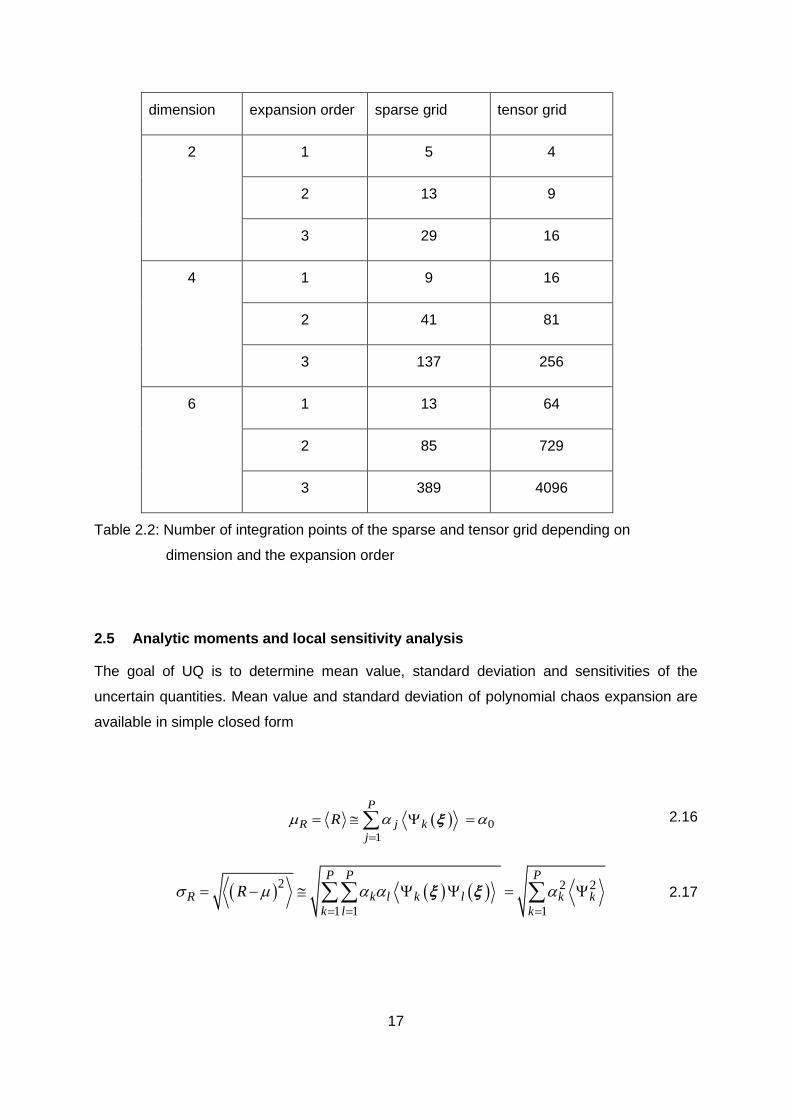
Large reduction of the number of collocation points for the case of moderately large number
of uncertain parameters can be achieved using sparse tensor product spaces as first
proposed by Smolyak [8]. This reduction can be seen in Table 2.2, where the comparison
between sparse and tensor grids is given [9].

16
dimension expansion order nested grid tensor grid
2 1 9 4
5 49 36
13 225 196
3 1 27 8
5 343 216
13 3375 2744
4 1 81 16
5 2401 1296
13 50625 38416
Table 2.1: Number of integration points depending on grid type, dimension and the
expansion order
17
dimension expansion order sparse grid tensor grid
2 1 5 4
2 13 9
3 29 16
4 1 9 16
2 41 81
3 137 256
6 1 13 64
2 85 729
3 389 4096
Table 2.2: Number of integration points of the sparse and tensor grid depending on
dimension and the expansion order
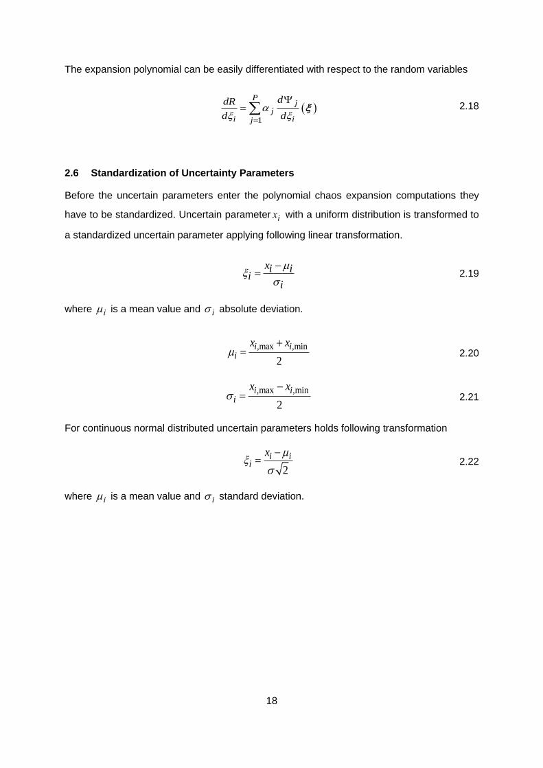
2.5 Analytic moments and local sensitivity analysis
The goal of UQ is to determine mean value, standard deviation and sensitivities of the
uncertain quantities. Mean value and standard deviation of polynomial chaos expansion are
available in simple closed form
0
1
P
R j k
j
R
2.16
2 2 2
1 1 1
P P P
R k l k l k kk l k
R
2.17
18
The expansion polynomial can be easily differentiated with respect to the random variables
1
Pj
ji ij
ddR
d d
2.18
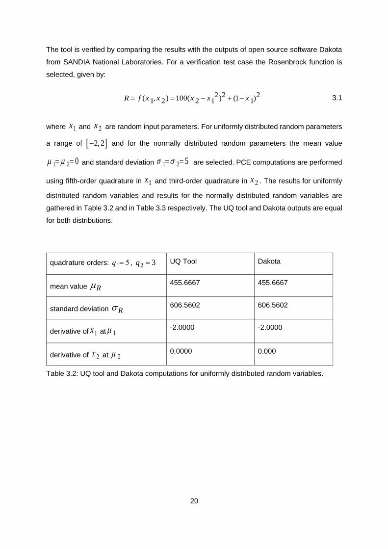
2.6 Standardization of Uncertainty Parameters
Before the uncertain parameters enter the polynomial chaos expansion computations they
have to be standardized. Uncertain parameter ix with a uniform distribution is transformed to
a standardized uncertain parameter applying following linear transformation.
xi i
ii
2.19
where i is a mean value and i absolute deviation.
,max ,min
2
i ii
x x 2.20
,max ,min
2
i ii
x x 2.21
For continuous normal distributed uncertain parameters holds following transformation
2
i i
i
x 2.22
where i is a mean value and i standard deviation.

19
3 Tool implementation and verification
The UQ tool implementation is done in MATLAB and is based on theory described in chapter
2. The tool can work with up to 10 uncertain input parameters, which can be uniformly or
normally distributed. The tool start inputs and end outputs are given in Table 3.1.
Tool start inputs: Tool end outputs:
bounds of ,i ia b each uncertain input parameter
ix (uniform distribution) or
mean value i and standard deviation i of each
uncertain input parameter ix (normal distribution)
quadrature order in each dimension iq
response mean value R
response standard deviation
R
response derivatives i
i
dR
dx
Table 3.1: UQ tool start inputs and end outputs
Since the tool is performing numerical integration of Eq. 2.15 2.15, it defines the integration
points, i.e. uncertain parameter values for which examined function have to be evaluated.
Once the tool receives the function (response) values, it computes the output uncertainties.
The tool computation steps are illustrated in Figure 3.1. The computation time of the output
uncertainties depends on the selected quadrature order and number of dimensions, in other
words the number of the polynomial evaluations equals the number of integration points.
Figure 3.1: UQ tool computation steps
Start Inputs
Tool
Script 1
List of uncertain parameter
values
Function evaluation
List of function values
Tool
Script 2
End Outputs
(UQ)
20
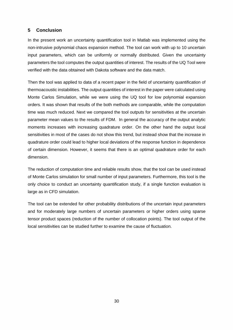
The tool is verified by comparing the results with the outputs of open source software Dakota
from SANDIA National Laboratories. For a verification test case the Rosenbrock function is
selected, given by:
2 2 2( , ) 100( ) (1 )1 2 2 1 1 R f x x x x x 3.1
where 1x and x2 are random input parameters. For uniformly distributed random parameters
a range of 2,2 and for the normally distributed random parameters the mean value
1 2 0 and standard deviation 1 2 5 are selected. PCE computations are performed
using fifth-order quadrature in 1x and third-order quadrature in 2x . The results for uniformly
distributed random variables and results for the normally distributed random variables are
gathered in Table 3.2 and in Table 3.3 respectively. The UQ tool and Dakota outputs are equal
for both distributions.
quadrature orders: 1 5q , 2 3q UQ Tool Dakota
mean value R 455.6667 455.6667
standard deviation R 606.5602 606.5602
derivative of 1x at 1 -2.0000 -2.0000
derivative of 2x at 2 0.0000 0.000
Table 3.2: UQ tool and Dakota computations for uniformly distributed random variables.

21
quadrature orders: 1 5q , 2 3q UQ Tool Dakota
mean value R 1.9003e+5 1.9003e+5
standard deviation R 6.1394e+5 6.1394e+5
derivative of 1x at 1 -2.0000 -2.0000
derivative of 2x at 2 0.0000 0.0000
Table 3.3: UQ tool and Dakota computations for normally distributed random variables.
The response function R (PCE output-polynomial), which can is extracted using Script 3 is a
very good approximation of the Rosenbrock function on the selected domain. The surfaces of
both analytical functions are identical, which can be seen in the Figure 3.2.
Figure 3.2: The plot of the Rosenbrock function and the response function (indistinguishable)

22
4 Uncertainty quantification of eigenvalues in thermoacoustics
Uncertainty quantification is a growing field with broad applications to a variety of engineering
fields. This chapter deals with a specific engineering problem, used here as an application test
case of the UQ tool. The test case is based on data of a recent scientific paper about
uncertainty quantification of thermoacoustic instabilities in a turbulent swirled combustor with
two configurations (C4, C8) [10]. In the paper authors use adjoints and Monte Carlo
simulations, we will use PCE and compare results.
The uncertainties considered in the test case are: the magnitude of the outlet reflection
coefficient 1x , the phase of the outlet reflection coefficient 2x , the gain of the flame transfer
function 3x and the time delay 3x . These four independent input parameters are uniformly
distributed within the bounds given in Table 4.1. The output angular frequency r or in growth
rate i of thermoacoustic instabilities are computed with a Helmholtz solver.
uniform distributed input uncertainties: bounds:
magnitude of the outlet reflection coefficient 1x 0.6 ± 10% [-]
the phase of the outlet reflection coefficient 2x π ± 10% [rad]
gain of the flame transfer function 3x 1.5 ± 10% [-]
flame time delay 4x 4.73e-3 ± 10% [s]
Table 4.1: Bounds of the input uncertainties
Firstly, the results are evaluated using the tool. PCE-computations are performed for three
different quadrature orders, including second, third and fourth order in each of the input
dimensions. The computation time of the output uncertainties depends on the selected
quadrature order (see chapter 3). Thus to compute the output uncertainties in angular
frequency r or in growth rate i on a conventional laptop2 it takes about 30 minutes for
second order, about 2.3 hours for third order and about 6.6 hours for fourth order quadrature
2 Intel Celeron CPU 1005M 1.9GHZ, 4,0 GB RAM

23
The output uncertainties are then quantified again, using method from the paper (Monte Carlo
simulations), in which the Helmholtz solver performs calculations with repeated random
sampling. For the purposes of this test 10 000 random input samples are fed. The computation
time of the simulation takes more than 14 hours on the same computer, which is a way slower
than PCE.
The results of PCE and Monte Carlo simulation are listed in Appendix 1 in Tables A.1 - A.2 for
configuration C4, and in Tables A.3 - A.4, for configuration C8. Both methods give nearly the
same results, the percentage differences between them are given in Tables 4.2 - 4.3, for
configuration C4, and in Tables 4.4 - 4.5, for configuration C8. In general variation of the
quadrature orders shows that the higher the order - the better the results. The differences
between the orders, however, stay relatively low.
UQ Tool vs. Monte Carlo
quadrature order 4 x 2nd order 4 x 3rd order 4 x 4th order
mean value R -0,03% -0,03% -0,03%
standard deviation R -1,23% -0,83% -0,47%
Table 4.2: Comparison of the UQ Tool results to the Monte Carlo results for
angular frequency r (configuration C4)
UQ Tool vs Monte Carlo
quadrature order 4 x 2nd order 4 x 3rd order 4 x 4th order
mean value R -0,37% -0,37% -0,34%
standard deviation R 0,15% -0,22% -0,05%
Table 4.3: Comparison of the UQ Tool results to the Monte Carlo results for
growth rate i (configuration C4)

24
UQ Tool vs Monte Carlo
quadrature order 4 x 2nd order 4 x 3rd order 4 x 4th order
mean value R 0,01% 0,01% 0,01%
standard deviation R -1,26% -0,88% -0,82%
Table 4.4: Comparison of the UQ Tool results to the Monte Carlo results for
angular frequency r (configuration C8)
UQ Tool vs Monte Carlo
quadrature order 4 x 2nd order 4 x 3rd order 4 x 4th order
mean value R -0,15% -0,13% -0,16%
standard deviation R 0,69% 0,47% 0,32%
Table 4.5: Comparison of the UQ Tool results to the Monte Carlo results for
growth rate i (configuration C8)

25
The next tool outputs are partial derivatives of the response function with respect to the input
parameters at the parameter mean values i . Their reliability is verified by the finite difference
method (FDM). The numerical solution for partial derivate using FDM is defined as
( ) ( )
2i
i i
i
R x h R x hdR
dx h
4.1
where 10 6ih x e . The results are given in Appendix A in Tables A.5 - A.8. The percentage
differences between the tool results and results obtained by the finite differences method are
listed in Table 4.6 - 4.9. The lowest value in each dimension is marked bold.
The results for angular frequency r in Tables 4.6 - 4.7 show, that in some cases the
difference decreases with increasing quadrature order, while in other cases the difference
increases. However, we can say that is better to select higher order for all dimensions, to
achieve the optimal results (to avoid the outliers). Here, the fourth quadrature order seems to
be the optimal one, since it gives the results with less than 1% difference to the FDM for all
dimensions, for both configurations.
UQ Tool vs FDM
quadrature order 4 x 2nd 4 x 3rd 4 x 4th
11
dR
dx
1,41% 0,02% -0,15%
22
dR
dx
-2,02% -0,48% -0,19%
33
dR
dx
-1,04% 0,13% 0,11%
44
dR
dx
0,58% 0,60% 0,36%
Table 4.6: Comparison of response derivatives for angular frequency r (configuration C4)

26
UQ Tool vs FDM
quadrature order 4 x 2nd 4 x 3rd 4 x 4th
11
dR
dx
0,17% -0,04% 0,05%
22
dR
dx
7,15% 4,85% 0,10%
33
dR
dx
-0,59% -0,78% 0,92%
44
dR
dx
-0,13% 0,49% -0,02%
Table 4.7: Comparison of response derivatives for angular frequency r (configuration C8)
Results for the growth rate i , given in Tables 4.84.6 - 4.9 showed larger deviations, so PCE-
computations were made for two additional quadrature orders (4 x 5th, 4 x 6th). Since the
result values fluctuate around the FDM value, it is hard to say that the difference either
increases or decreases with the increasing quadrature order. For configuration C4 in Table 4.8
it can be assumed that the 5th quadrature order is the optimal one, while the results for lower
orders and higher order show larger or smaller fluctuation. Similar assumption can be made
also for results for configuration C4, given in Table 4.8, where the 4th quadrature order is the
optimal one. For a better representation of the expansion order influence on UQ Figure B.1 (as
an example) is added to Appendix 2 and it shows the response function in dependence of the
magnitude of the outlet reflection coefficient 1x for different quadrature orders (configuration
C8). On Figure B.1 can be seen that increase in polynomial chaos expansion order could lead
to higher local deviations of the response function in dependence of certain dimension.
In general we can say, that the local sensitivity and FDM results were still comparable,
however, increase in polynomial chaos expansion order did not necessarily result in lower
differences.

27
UQ Tool vs FDM
q. order 4 x 2nd 4 x 3rd 4 x 4th 4 x 5th 4 x 6th
11
dR
dx
0,17% -0,14% -0,71% 0,00% -4,42%
22
dR
dx
1,14% 0,50% 0,86% 0,00% 1,27%
33
dR
dx
2,18% 0,09% 2,76% 0,00% -1,00%
44
dR
dx
-0,31% -0,53% 1,46% 0,02% 1,79%
Table 4.8: Comparison of response derivatives for growth rate i (configuration C4)
UQ Tool vs FDM
q. order 4 x 2nd 4 x 3rd 4 x 4th 4 x 5th 4 x 6th
11
dR
dx
6,73% -3,40% -3,00% -3,19% 5,56%
22
dR
dx
0,26% -0,17% -0,16% -0,53% -0,18%
33
dR
dx
-0,11% -0,31% -0,55% -0,36% -0,05%
44
dR
dx
2,36% -2,69% 1,05% 5,48% 1,36%
Table 4.9: Comparison of response derivatives for growth rate i (configuration C8)

28
In addition to the response outputs computed above, the response PDF for different quadrature
orders is calculated and compared to PDF of the growth rate presented by C.Silva et al [10].
For a single uncertainty input parameter 1x , it is possible to calculate the PDF of the response
( )iRf using expression [11]
1
1 1( ) ( ( )) ( ( ))i i iR Xi
df R f R
d
4.2
where 1X
f stands for the PDF of the input variable. Since there is more than one input
parameters considered here, the PDF is computed using Monte Carlo simulations applied on
the PCE-output polynomial (using Script 3). In Figure 4.1 and Figure 4.2 the computed PDFs
of the growth rate i for the two methods are compared. The results are virtually identical for
all three orders considered.
While the Monte Carlo simulation with the Helmholtz solver takes several hours (as applied in
[10]), the simulation with the PCE-response polynomial only takes a few minutes. It is clear,
that evaluation of PCE-response polynomial is a way faster than the evaluation of original
function (Helmholtz solver). The speed up increases with complexity of the original function.
Figure 4.1: Growth rate PDF for different quadrature orders, configuration C4

29
Figure 4.2: Growth rate PDF for different quadrature orders, configuration C8
30
5 Conclusion
In the present work an uncertainty quantification tool in Matlab was implemented using the
non-intrusive polynomial chaos expansion method. The tool can work with up to 10 uncertain
input parameters, which can be uniformly or normally distributed. Given the uncertainty
parameters the tool computes the output quantities of interest. The results of the UQ Tool were
verified with the data obtained with Dakota software and the data match.
Then the tool was applied to data of a recent paper in the field of uncertainty quantification of
thermoacoustic instabilities. The output quantities of interest in the paper were calculated using
Monte Carlos Simulation, while we were using the UQ tool for low polynomial expansion
orders. It was shown that results of the both methods are comparable, while the computation
time was much reduced. Next we compared the tool outputs for sensitivities at the uncertain
parameter mean values to the results of FDM. In general the accuracy of the output analytic
moments increases with increasing quadrature order. On the other hand the output local
sensitivities in most of the cases do not show this trend, but instead show that the increase in
quadrature order could lead to higher local deviations of the response function in dependence
of certain dimension. However, it seems that there is an optimal quadrature order for each
dimension.
The reduction of computation time and reliable results show, that the tool can be used instead
of Monte Carlos simulation for small number of input parameters. Furthermore, this tool is the
only choice to conduct an uncertainty quantification study, if a single function evaluation is
large as in CFD simulation.
The tool can be extended for other probability distributions of the uncertain input parameters
and for moderately large numbers of uncertain parameters or higher orders using sparse
tensor product spaces (reduction of the number of collocation points). The tool output of the
local sensitivities can be studied further to examine the cause of fluctuation.
31
6 Bibliography
[1] https://en.wikipedia.org/wiki/Uncertainty_quantification, (2016, October).
[2] http://mathworld.wolfram.com/OrthogonalPolynomials.html, (2016, October).
[3] R. Askey and J. Wilson. Some basic hypergeometric polynomials that generalize Jacobi polynomials. In Mem. Amer. Math. Soc. 319, Providence, RI, 1985. AMS. 23.
[4] https://en.wikipedia.org/wiki/Legendre_polynomials, (2016, October).
[5] https://en.wikipedia.org/wiki/Hermite_polynomials, (2016, October).
[6] B. M. Adams, K. R. Dalbey, M. S. Eldred, L. P. Swiler, W. J. Bohnhoff, J. P. Eddy, D. M. Vigil, P. D. Hough, and S. Lefantzi. DAKOTA, A Multilevel Parallel Object-Oriented Framework for Design Optimization, Parameter Estimation, Uncertainty Quantification, and Sensitivity Analysis. Version 5.2.
[7] https://people.sc.fsu.edu/~jburkardt/f_src/patterson_rule/patterson_rule.html, (2016, October)
[8] S.A. Smolyak. Quadrature and interpolation formulas for tensor products of certain classes of functions, Dokl. Akad. Nauk SSSR, 4:240–243, 1963. 30
[9] http://sparse-grids.de/, (2016, October)
[10] Uncertainty quantification of growth rates of thermoacoustic instability by an adjoint Helmholz solver; Camilo F.Silva, Thomas Runte, Wolfgang Polfike, Luca Magri, June 13-17, 2016
[11] https://en.wikipedia.org/wiki/Probability_density_function. (2016, October).

32
A Appendix 1
Here the results of tool, Monte Carlo simulation and finite difference method are given.
UQ Tool Monte Carlo
quadrature order 4 x 2nd 4 x 3rd 4 x 4th
mean value R 147.7648 147.7643 147.7682 147.8064
standard deviation R 3.3217 3.3351 3.3472 3.3630
Table A.1 : Results for angular frequency r (configuration C4)
UQ Tool Monte Carlo
quadrature order 4 x 2nd 4 x 3rd 4 x 4th
mean value R 109.6342 109.6410 109.6679 110.0443
standard deviation R 17.9473 17.8812 17.9122 17.9208
Table A.2: Results for growth rate i (configuration C4)
UQ Tool Monte Carlo
quadrature order 4 x 2nd 4 x 3rd 4 x 4th
mean value R 129.6169 129.6175 129.6161 129.6003
standard deviation R 3.0657 3.0776 3.0794 3.1049
Table A.3: Results for angular frequency r (configuration C8)

33
UQ Tool Monte Carlo
quadrature order 4 x 2nd 4 x 3rd 4 x 4th
mean value R 109.2022 109.2255 109.1888 109.3649
standard deviation R 13.7553 13.7258 13.7056 13.6617
Table A.4: Results for growth rate i (configuration C8)
UQ Tool FDM
quadrature order 4 x 2nd 4 x 3rd 4 x 4th
11
dR
dx
20.1336 19.8527 19.844 19.8490
22
dR
dx
-3.7077 -3.7644 -3.7752 -3.7825
33
dR
dx
-3.2833 -3.3218 -3.3210 -3.3174
44
dR
dx
-11656.3458 -11659.0547 -11630.6275 -11589.2706
Table A.5: Response derivatives for angular frequency r (configuration C4)

34
UQ Tool FDM
quadrature order 4 x 2nd 4 x 3rd 4 x 4th
11
dR
dx
17.8320 17.7943 17.8095 17.8009
22
dR
dx
1.5870 1.5451 1.4751 1.4736
33
dR
dx
-0,5955 -0.5943 -0.6045 -0.5990
44
dR
dx
-10914.8268 -10983.0256
-10926.8612 -10928.9282
Table A.6: Response derivatives for angular frequency r (configuration C8)

35
UQ Tool FDM
q.order 4 x 2nd 4 x 3rd 4 x 4th 5 x 5th 6 x 6th
11
dR
dx
39.6773 39.5555
39.73306 39.6105 37.8601 39.6109
22
dR
dx
75.6938 75.2060 75.4714 74.8275 75.7779 74.8288
33
dR
dx
56.0188 54.8464 56.3106 54.7962 54.2508 54.7975
44
dR
dx
-
38010.4480
-
37925.0564
-
38682.3518
-
38133.7644
-
38807.8577
-
38126.6416
Table A.7: Response derivatives for growth rate i (configuration C4)

36
UQ Tool FDM
q.order 4 x 2nd 4 x 3rd 4 x 4th 4 x 5th 4 x 6th
11
dR
dx
-16.5443 -14.9068
-14.9686 -14.9399 -16.2896 -15.4316
22
dR
dx
67.2836 66.9914 66.9984 66.7502 66.9893 67.1081
33
dR
dx
56.6548 56.5463 56.4065 56.5142 56.6901 56.7194
44
dR
dx
-
14267.5922
-
13556.8445
-
14077.3620
-
14694.7160
-
14121.1743
-
13931.3442
Table A.8: Response derivatives for growth rate i , configuration C8

37
B Appendix 2
Here the response function in dependence of the magnitude of the outlet reflection coefficient
1x for different quadrature orders is given, while for other input variables mean values ( 2 ,
3 , 4 ) were used (configuration C8). The lack vertical line shows the mean value of the
magnitude of the outlet reflection coefficient ( 1 ).
Figure B.1: The response function in dependence of the magnitude of the outlet reflection
coefficient 1x for different quadrature orders