Master of Science ThesisStockholm, Sweden 2010

TRITA-ICT-EX-2010:125

D A N I E L T U R U L L T O R R E N T S

Open Source Traffic Analyzer

K T H I n f o r m a t i o n a n dC o m m u n i c a t i o n T e c h n o l o g y

Abstract

Proper traffic analysis is crucial for the development of network systems, services and proto-cols. Traffic analysis equipment is often based on costly dedicated hardware, and uses proprietarysoftware for traffic generation and analysis. The recent advances in open source packet processing,with the potential of generating and receiving packets using a regular Linux computer at 10 Gb/sspeed, opens up very interesting possibilities in terms of implementing a traffic analysis systembased on open-source Linux.

The pktgen software package for Linux is a popular tool in the networking community forgenerating traffic loads for network experiments. Pktgen is a high-speed packet generator, runningin the Linux kernel very close to the hardware, thereby making it possible to generate packets withvery little processing overhead. The packet generation can be controlled through a user interfacewith respect to packet size, IP and MAC addresses, port numbers, inter-packet delay, and so on.

Pktgen was originally designed with the main goal of generating packets at very high rate.However, when it comes to support for traffic analysis, pktgen has several limitations. One ofthe most important characteristics of a packet generator is the ability to generate traffic at aspecified rate. Pktgen can only do this indirectly, by inserting delays between packets. Moreover,the timer granularity prevents precise control of the transmission rate, something which severelyreduces pktgen’s usefulness as an analysis tool. Furthermore, pktgen lacks support for receive-side analysis and statistics generation. This is a key issue in order to convert pktgen into a usefulnetwork analyser tool.

In this paper, improvements to pktgen are proposed, designed, implemented and evaluated,with the goal of evolving pktgen into a complete and efficient network analysis tool. The ratecontrol is significantly improved, increasing the resolution and improving the usability by makingit possible to specify exactly the sending rate. A receive-side tool is designed and implementedwith support for measurement of number of packets, throughput, inter-arrival time, jitter andlatency. The design of the receiver takes advantage of SMP systems and new features on modernnetwork cards, in particular support for multiple receive queues and CPU scheduling. This makesit possible to use multiple CPUs to parallelize the work, improving the overall capacity of thetraffic analyser.

A significant part of the work has been spent on investigating low-level details of Linuxnetworking. From this work we draw some general conclusions related to high speed packetprocessing in SMP systems. In particular, we study how the packet processing capacity per CPUdepends on the number of CPUs.

This work consists of minimal set of kernel patches to pktgen.

Contents

Contents i

List of Figures iii

List of Tables v

1 Introduction 11.1 Goals . . . . . . . . . . . . . . . . . . . . . . . . . . . . . . . . . . . . . . . . . . . . . 21.2 Thesis outline . . . . . . . . . . . . . . . . . . . . . . . . . . . . . . . . . . . . . . . . . 2

2 Background study 32.1 Network analysis . . . . . . . . . . . . . . . . . . . . . . . . . . . . . . . . . . . . . . . 3

2.1.1 Methodologies . . . . . . . . . . . . . . . . . . . . . . . . . . . . . . . . . . . . 32.1.2 Custom hardware based . . . . . . . . . . . . . . . . . . . . . . . . . . . . . . . 32.1.3 Software based . . . . . . . . . . . . . . . . . . . . . . . . . . . . . . . . . . . . 42.1.4 Mixed solution . . . . . . . . . . . . . . . . . . . . . . . . . . . . . . . . . . . . 82.1.5 Metrics used in network analysis . . . . . . . . . . . . . . . . . . . . . . . . . . 82.1.6 Technologies . . . . . . . . . . . . . . . . . . . . . . . . . . . . . . . . . . . . . 10

2.2 Linux Kernel . . . . . . . . . . . . . . . . . . . . . . . . . . . . . . . . . . . . . . . . . 102.2.1 Linux overview . . . . . . . . . . . . . . . . . . . . . . . . . . . . . . . . . . . . 102.2.2 Communications between User-space to kernel . . . . . . . . . . . . . . . . . . 102.2.3 Network subsystem . . . . . . . . . . . . . . . . . . . . . . . . . . . . . . . . . . 12

2.3 Pktgen study . . . . . . . . . . . . . . . . . . . . . . . . . . . . . . . . . . . . . . . . . 132.3.1 About . . . . . . . . . . . . . . . . . . . . . . . . . . . . . . . . . . . . . . . . . 132.3.2 Pktgen Control and visualization . . . . . . . . . . . . . . . . . . . . . . . . . . 142.3.3 Pktgen operation . . . . . . . . . . . . . . . . . . . . . . . . . . . . . . . . . . . 15

3 Design 193.1 Requirements . . . . . . . . . . . . . . . . . . . . . . . . . . . . . . . . . . . . . . . . . 19

3.1.1 Not used parameters . . . . . . . . . . . . . . . . . . . . . . . . . . . . . . . . . 193.2 Architecture . . . . . . . . . . . . . . . . . . . . . . . . . . . . . . . . . . . . . . . . . . 203.3 Receiver metrics . . . . . . . . . . . . . . . . . . . . . . . . . . . . . . . . . . . . . . . 20

3.3.1 Metrics computation . . . . . . . . . . . . . . . . . . . . . . . . . . . . . . . . . 203.3.2 Data collection . . . . . . . . . . . . . . . . . . . . . . . . . . . . . . . . . . . . 22

3.4 Application interface . . . . . . . . . . . . . . . . . . . . . . . . . . . . . . . . . . . . . 223.4.1 User Control . . . . . . . . . . . . . . . . . . . . . . . . . . . . . . . . . . . . . 223.4.2 Measurement visualization . . . . . . . . . . . . . . . . . . . . . . . . . . . . . . 22

3.5 Operation . . . . . . . . . . . . . . . . . . . . . . . . . . . . . . . . . . . . . . . . . . . 233.5.1 Initialization . . . . . . . . . . . . . . . . . . . . . . . . . . . . . . . . . . . . . 233.5.2 Packet transmission . . . . . . . . . . . . . . . . . . . . . . . . . . . . . . . . . 23

i

3.5.3 Packet reception . . . . . . . . . . . . . . . . . . . . . . . . . . . . . . . . . . . 24

4 Implementation 274.1 Processing the incoming packet . . . . . . . . . . . . . . . . . . . . . . . . . . . . . . . 27

4.1.1 Accessing data of the packet . . . . . . . . . . . . . . . . . . . . . . . . . . . . 284.1.2 Saving the statistics . . . . . . . . . . . . . . . . . . . . . . . . . . . . . . . . . 294.1.3 Measuring time . . . . . . . . . . . . . . . . . . . . . . . . . . . . . . . . . . . . 30

4.2 Auto-configuration of the receiver . . . . . . . . . . . . . . . . . . . . . . . . . . . . . . 314.2.1 Sending . . . . . . . . . . . . . . . . . . . . . . . . . . . . . . . . . . . . . . . . 314.2.2 Receiver . . . . . . . . . . . . . . . . . . . . . . . . . . . . . . . . . . . . . . . . 31

4.3 Displaying the results . . . . . . . . . . . . . . . . . . . . . . . . . . . . . . . . . . . . 324.4 Increasing the performance modifying the network subsystem . . . . . . . . . . . . . . 344.5 Adjusting the transmission throughput . . . . . . . . . . . . . . . . . . . . . . . . . . . 34

5 Evaluation 375.1 Equipment and scenario . . . . . . . . . . . . . . . . . . . . . . . . . . . . . . . . . . . 37

5.1.1 Hardware . . . . . . . . . . . . . . . . . . . . . . . . . . . . . . . . . . . . . . . 375.1.2 Software . . . . . . . . . . . . . . . . . . . . . . . . . . . . . . . . . . . . . . . . 375.1.3 Scenarios . . . . . . . . . . . . . . . . . . . . . . . . . . . . . . . . . . . . . . . 375.1.4 Parameters under study . . . . . . . . . . . . . . . . . . . . . . . . . . . . . . . 38

5.2 Validation and Calibration . . . . . . . . . . . . . . . . . . . . . . . . . . . . . . . . . . 385.2.1 Receiver throughput . . . . . . . . . . . . . . . . . . . . . . . . . . . . . . . . . 385.2.2 Inter-arrival time and jitter . . . . . . . . . . . . . . . . . . . . . . . . . . . . . 405.2.3 Latency . . . . . . . . . . . . . . . . . . . . . . . . . . . . . . . . . . . . . . . . 43

5.3 Performance . . . . . . . . . . . . . . . . . . . . . . . . . . . . . . . . . . . . . . . . . . 445.3.1 Comparison between the different methods of collecting statistics . . . . . . . . 445.3.2 Header split or not split . . . . . . . . . . . . . . . . . . . . . . . . . . . . . . . 455.3.3 Trade-offs between single-system and dual-system implementations . . . . . . . 465.3.4 Implications of low performance . . . . . . . . . . . . . . . . . . . . . . . . . . 46

6 Conclusions 496.1 Future work . . . . . . . . . . . . . . . . . . . . . . . . . . . . . . . . . . . . . . . . . . 50

Bibliography 51

A Source code and scripts 55A.1 Kernel patching and compiling . . . . . . . . . . . . . . . . . . . . . . . . . . . . . . . 55A.2 Summary of the new commands added in pktgen . . . . . . . . . . . . . . . . . . . . . 55

A.2.1 Transmitter . . . . . . . . . . . . . . . . . . . . . . . . . . . . . . . . . . . . . . 56A.2.2 Receiver . . . . . . . . . . . . . . . . . . . . . . . . . . . . . . . . . . . . . . . . 56

A.3 Examples of pktgen configuration scripts . . . . . . . . . . . . . . . . . . . . . . . . . . 56

ii

List of Figures

2.1 Spirent SmartBits . . . . . . . . . . . . . . . . . . . . . . . . . . . . . . . . . . . . . . . . 52.2 A split view of the kernel. Source [49] . . . . . . . . . . . . . . . . . . . . . . . . . . . . . 112.3 Network subsystem stack . . . . . . . . . . . . . . . . . . . . . . . . . . . . . . . . . . . . 122.4 Packet path in the reception. Source [50] . . . . . . . . . . . . . . . . . . . . . . . . . . . 132.5 pktgen’s thread main loop flow graph . . . . . . . . . . . . . . . . . . . . . . . . . . . . . 162.6 Pktgen_xmit() flow graph . . . . . . . . . . . . . . . . . . . . . . . . . . . . . . . . . . . . 17

3.1 Latency . . . . . . . . . . . . . . . . . . . . . . . . . . . . . . . . . . . . . . . . . . . . . . 213.2 Flow chart of reception in time statistics. . . . . . . . . . . . . . . . . . . . . . . . . . . . 25

4.1 Reading parameters performance . . . . . . . . . . . . . . . . . . . . . . . . . . . . . . . . 284.2 Comparison between packet handler and hook . . . . . . . . . . . . . . . . . . . . . . . . . 344.3 Throughput with delays. Gigabit Link . . . . . . . . . . . . . . . . . . . . . . . . . . . . . 354.4 Throughput with delays. 10 Gigabit Link . . . . . . . . . . . . . . . . . . . . . . . . . . . 36

5.1 Maximal transmission rate . . . . . . . . . . . . . . . . . . . . . . . . . . . . . . . . . . . . 395.2 Test results. Different CPU receiving . . . . . . . . . . . . . . . . . . . . . . . . . . . . . . 405.3 Inter-arrival and Jitter with default values . . . . . . . . . . . . . . . . . . . . . . . . . . . 415.4 Inter-arrival and Jitter with different spin time . . . . . . . . . . . . . . . . . . . . . . . . 425.5 Inter-arrival and Jitter with different frequency . . . . . . . . . . . . . . . . . . . . . . . . 435.6 Inter-arrival and Jitter for the original module . . . . . . . . . . . . . . . . . . . . . . . . 435.7 Latency test with 1G network card . . . . . . . . . . . . . . . . . . . . . . . . . . . . . . . 445.8 Latency test with 10G network card . . . . . . . . . . . . . . . . . . . . . . . . . . . . . . 445.9 Comparison of losses of the three different types of statistics . . . . . . . . . . . . . . . . . 455.10 Invalid tests due to bad performance . . . . . . . . . . . . . . . . . . . . . . . . . . . . . . 47

iii

List of Tables

2.1 Traffic measurements at IxNetwork . . . . . . . . . . . . . . . . . . . . . . . . . . . . . . . 4

5.1 Test scenarios . . . . . . . . . . . . . . . . . . . . . . . . . . . . . . . . . . . . . . . . . . . 385.2 Test parameters. Different number of CPUs . . . . . . . . . . . . . . . . . . . . . . . . . . 395.3 Test results. Different CPU receiving . . . . . . . . . . . . . . . . . . . . . . . . . . . . . . 415.4 Test parameters. Header split test . . . . . . . . . . . . . . . . . . . . . . . . . . . . . . . 455.5 Test Results. Header Split . . . . . . . . . . . . . . . . . . . . . . . . . . . . . . . . . . . . 455.6 Test Results. Header Split in hook kernel . . . . . . . . . . . . . . . . . . . . . . . . . . . 465.7 Results of TX/RX in the same machine . . . . . . . . . . . . . . . . . . . . . . . . . . . . 46

v

Chapter 1

Introduction

Proper traffic analysis equipment is crucial for the development of network systems, servicesand protocols. Traffic analysis equipment is often based on costly dedicated hardware, and usesproprietary software for traffic generation and analysis. The recent advances in open source packetprocessing, with the potential of generating and receiving packets using a regular Linux PC at 10Gb/s speed, opens up very interesting possibilities in terms of implementing a traffic analysis systembased on an open-source Linux system.

Open source traffic analysers can be used in academic and research communities in order tounderstand better networks and systems. This can be used to create better hardware and operatingsystems for the future.

Processors manufactures are focusing their designs in systems with multiple processors, calledSMP systems, instead of increasing the processor clock. Processors with up to 4 cores are becomingcommon in the commodity market. In order to take advantage of SMP systems, new feature suchmultiple queues are added to network cards. This allows multiple CPUs to work concurrently withoutany interference. Each CPU is in charge of one queue, making possible the parallelization of the packetprocessing of a single interface. This feature can be used to increase the performance of the toolsthat analyse high speed networks.

There are different options in the open source community of Linux to analyse network behaviour,but most of them are user-space applications (netperf, iperf ...). They have advantages in termsof usability but also drawbacks in terms of performance. Managing small packets in high speednetworks requires a lot of process, and all the resources of the system are needed. In this case, user-space applications do not achieve higher rates. The main problem is that there is a high overheaddue to the entire network stack.

The Pktgen software package for Linux is a popular tool in the networking community for gener-ating traffic loads for network experiments. Pktgen is a high-speed packet generator, running in theLinux kernel very close to the hardware, thereby making it possible to generate packets with verylittle processing overhead. The packet generation can be controlled through the user interface withrespect to packet size, IP and MAC addresses, port numbers, inter-packet delay, and so on.

There is currently no receive-side counterpart to Pktgen. That is, an application that receivespackets on an interface, performs analysis on the packets received, and collects statistics. Pktgenhave the advantage that is a kernel module, which can bypass entire network overhead, resultingin better performance. Also, because it is inside the kernel can use resources of the system moreefficiently.

1

1.1 GoalsThe goals of this master thesis can be described as follows:

• Investigate the current solutions for traffic analyses

• Understand how Pktgen works

• Investigate how design and implement a network analyser inside the Linux Kernel, takingadvantage of the new features in the modern systems.

• Integrate the results in the current Pktgen module

• Evaluate and calibrate the behaviour of the module implemented

1.2 Thesis outlineThis work is organized as follows:

• Chapter 2 contains the background study. A study of the current network analysis tools andmethodologies is done. Also, a brief introduction of the Linux Kernel is presented. FinallyPktgen is studied in depth in order to understand how it works.

• Chapter 3 contains the requirements and the design of the traffic analyzer implemented withPktgen. The design includes the architecture, the receiver metrics and the application interface.Also an overview of the operation is presented.

• Chapter 4 contains some explanations of the modified code, as well as the new add-ons. More-over some test are included in order to justify its choice. Also explains how the design proposedin Chapter 3 is implemented.

• Chapter 5 evaluates the behaviour and performance of the implemented solution using differentreal tests. Some conclusions about the results of the test are drawn.

• Chapter 6 summarise the work and draws some conclusion of it. Moreover, some suggestionsfor the future work are provided.

2

Chapter 2

Background study

This chapter includes a study of the current network analysis tools and methodologies. Then,some of the used parameters of the network analysis tools are defined. Also, a brief introductionof the Linux Kernel is presented. Finally Pktgen is studied in depth in order to understand how itworks, in order to add new features to Pktgen.

2.1 Network analysis

2.1.1 Methodologies

Traditionally two different approaches are taken in order to analyse the network and its perfor-mance. The first one is custom hardware based solutions which are usually very expensive buthave a good performance. The second one is software based which it is cheaper and more flexible.It can run in general purpose systems, such as Personal Computers (PCs) but sometimes it hasproblems of performance at high speed networks. Also, in the recent years, a third solution based onnetwork processors appears between both of them.

In the following section, different solutions of different types will be introduced with a briefoverview.

2.1.2 Custom hardware based

Usually custom hardware based solutions are proprietary and very expensive due to its special-ization. It is the most popular approach for the industrial environment. Such solutions are designedto minimize the delays and increase the performance. All the functionalities are developed near thehardware in order to adjust the delays introduced by the operating system (OS) in general purposesystems.

These tools are configurable, but due to its specialization it is difficult to change its behaviour.Normally, the testing equipment is located at the ends of the sections to be tested.

2.1.2.1 Ixia - IxNetwork

Ixia [1] is the former Agilent. Ixia’s solutions are based on hardware and specialized equipment.Their products offer a wide range of testing tools for performance and compliance of communicationsequipment. Related with network analysis are IxNetwork and IxCharriot.

IxNetwork IxNetwork [2] is the solution for testing network equipment at its full capacity. Itallows simulating and tracking millions of traffic flows. Also there is a wizard to customize the traffic

3

and is able to generate up to 4 million traceable flows due to its scalability. It is focused in L2 andL3 protocols.

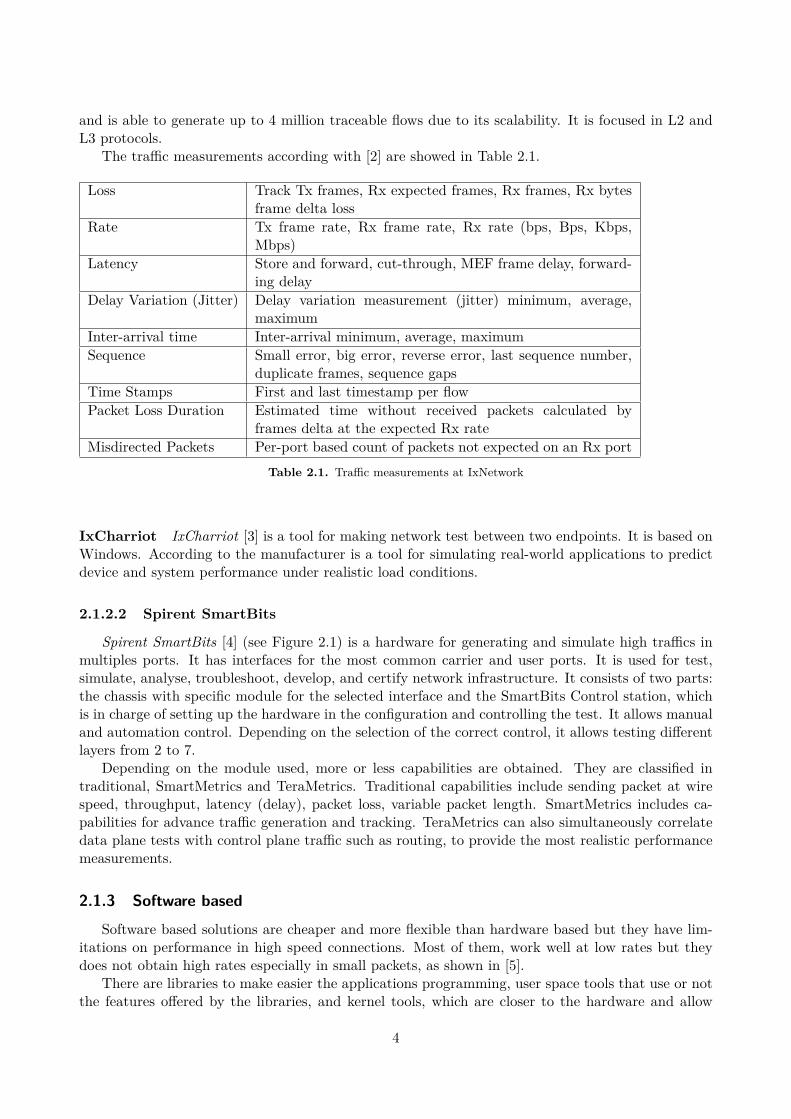
The traffic measurements according with [2] are showed in Table 2.1.

Loss Track Tx frames, Rx expected frames, Rx frames, Rx bytesframe delta loss

Rate Tx frame rate, Rx frame rate, Rx rate (bps, Bps, Kbps,Mbps)

Latency Store and forward, cut-through, MEF frame delay, forward-ing delay

Delay Variation (Jitter) Delay variation measurement (jitter) minimum, average,maximum

Inter-arrival time Inter-arrival minimum, average, maximumSequence Small error, big error, reverse error, last sequence number,

duplicate frames, sequence gapsTime Stamps First and last timestamp per flowPacket Loss Duration Estimated time without received packets calculated by

frames delta at the expected Rx rateMisdirected Packets Per-port based count of packets not expected on an Rx port

Table 2.1. Traffic measurements at IxNetwork

IxCharriot IxCharriot [3] is a tool for making network test between two endpoints. It is based onWindows. According to the manufacturer is a tool for simulating real-world applications to predictdevice and system performance under realistic load conditions.

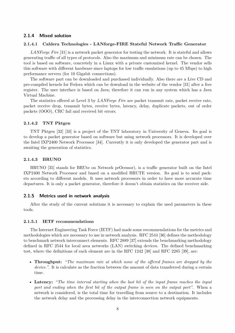
2.1.2.2 Spirent SmartBits

Spirent SmartBits [4] (see Figure 2.1) is a hardware for generating and simulate high traffics inmultiples ports. It has interfaces for the most common carrier and user ports. It is used for test,simulate, analyse, troubleshoot, develop, and certify network infrastructure. It consists of two parts:the chassis with specific module for the selected interface and the SmartBits Control station, whichis in charge of setting up the hardware in the configuration and controlling the test. It allows manualand automation control. Depending on the selection of the correct control, it allows testing differentlayers from 2 to 7.

Depending on the module used, more or less capabilities are obtained. They are classified intraditional, SmartMetrics and TeraMetrics. Traditional capabilities include sending packet at wirespeed, throughput, latency (delay), packet loss, variable packet length. SmartMetrics includes ca-pabilities for advance traffic generation and tracking. TeraMetrics can also simultaneously correlatedata plane tests with control plane traffic such as routing, to provide the most realistic performancemeasurements.

2.1.3 Software based

Software based solutions are cheaper and more flexible than hardware based but they have lim-itations on performance in high speed connections. Most of them, work well at low rates but theydoes not obtain high rates especially in small packets, as shown in [5].

There are libraries to make easier the applications programming, user space tools that use or notthe features offered by the libraries, and kernel tools, which are closer to the hardware and allow

4

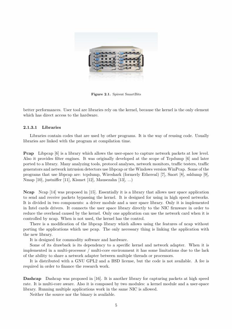
Figure 2.1. Spirent SmartBits

better performances. User tool are libraries rely on the kernel, because the kernel is the only elementwhich has direct access to the hardware.

2.1.3.1 Libraries

Libraries contain codes that are used by other programs. It is the way of reusing code. Usuallylibraries are linked with the program at compilation time.

Pcap Libpcap [6] is a library which allows the user-space to capture network packets at low level.Also it provides filter engines. It was originally developed at the scope of Tcpdump [6] and laterported to a library. Many analyzing tools, protocol analyses, network monitors, traffic testers, trafficgenerators and network intrusion detectors use libpcap or the Windows version WinPcap. Some of theprograms that use libpcap are: tcpdump, Wireshark (formerly Ethereal) [7], Snort [8], ssldump [9],Nmap [10], justniffer [11], Kismet [12], Mausezahn [13], ...)

Ncap Ncap [14] was proposed in [15]. Essentially it is a library that allows user space applicationto send and receive packets bypassing the kernel. It is designed for using in high speed networks.It is divided in two components: a driver module and a user space library. Only it is implementedin Intel cards drivers. It connects the user space library directly to the NIC firmware in order toreduce the overhead caused by the kernel. Only one application can use the network card when it iscontrolled by ncap. When is not used, the kernel has the control.

There is a modification of the libpcap library which allows using the features of ncap withoutporting the applications which use pcap. The only necessary thing is linking the application withthe new library.

It is designed for commodity software and hardware.Some of its drawback is its dependency to a specific kernel and network adapter. When it is

implemented in a multi-processor / multi-core environment it has some limitations due to the lackof the ability to share a network adapter between multiple threads or processors.

It is distributed with a GNU GPL2 and a BSD license, but the code is not available. A fee isrequired in order to finance the research work.

Dashcap Dashcap was proposed in [16]. It is another library for capturing packets at high speedrate. It is multi-core aware. Also it is composed by two modules: a kernel module and a user-spacelibrary. Running multiple applications work in the same NIC is allowed.

Neither the source nor the binary is available.

5

2.1.3.2 User Space tools

User space tools are on the top of the system architecture and usually have lower performanceand speed than kernel ones. They use system calls to use the resources of the system.

IPerf IPerf [17] is a classical Linux tool that allows testing the throughput of a network connectionbetween two nodes at application level. It can operate with TCP and UDP and returns the networkbandwidth of a given link with the given buffers. It makes some modifications in the buffers of thesystem in order to get the higher throughput. Also it allows setting customized values for the user.

A server is listening for incoming connection and the client starts the connection and measuresthe network bandwidth in a unidirectional way. It is possible to measure bidirectional traffic.

The statistics offered by IPerf are the amount of data transferred in a given interval, the averagethroughput, the jitter and the losses.

NetPerf Netperf [18] is a popular tool for benchmarking the network. It is created by IND Net-working Performance Team of Hewlett-Packard. It provides tests for both unidirectional throughput,and end-to-end latency. It is focused on sending bulk data using either TCP or UDP.

The only statistic offered by NetPerf is the throughput of the test. The latency has to be obtainedin an indirect way.

NetPIPE NetPIPE [19] is a benchmark tool for the network throughput. It sends messages withan incremental size in order to evaluate the throughput obtained with this message. It allows checkingthe OS parameters (socket buffer sizes, etc...) with messages of different size in order to optimizethem. Also allows identifying drop-outs in networking hardware and drivers.

The result of the test is a series that contains the message length, the times that it is send, thethroughput obtained and the time needed to send it. It generates a file with the output in order torepresent it.

Mausezahn Mausezahn [13] is a free traffic generator which allows sending whatever type of packetbecause the packets can be customized. It allows measuring the jitter between two hosts. It is basedin libpcap library (See 2.1.3.1).

The statistics obtained by Mausezahn are: timestamp, minimum jitter, average jitter, maximumjitter, estimated jitter, minimum delta RX, average delta RX, maximum delta RX, packet drop count(total) and packet disorder count (total).

Harpoon Harpoon [20] is a flow-level traffic generator. It can generate the distribution statisticsextracted from Netflow traces to generate flows which contains real Internet packet behaviour.

TPtest TPtest [21] is a tool for measuring the throughput speed of an Internet connection to andfrom different servers. It was originally developed by the Swedish government. It is used for evaluatethe quality of the service offered by the Internet Service Providers (ISP).

It allows measuring the TCP and UDP throughput (incoming and outgoing), UDP packet loss,UDP round trip times and UDP out-of-order packet reception.

ttcp Ttcp [22] is a command-line sockets-based benchmarking tool for measuring TCP and UDPperformance between two systems. It was developed in the BSD operation system in 1984. The codeis freely available.

6

nuttcp Nuttcp[23] is a tool for measuring the throughput of a network. It is a modification ofttcp. It allows adjusting the output throughput and the packet size. The results displayed are thethroughput archived, the packets received and the packets lost. Also it includes the load of thereceiver and the transmission node. Nuttcp can run as a server and pass all the results to the clientside. Then, it is not necessary to have access to the server.

RUDE/CRUDE RUDE [24] stands for Real-time UDP Data Emitter and CRUDE for Collectorfor RUDE. RUDE is a traffic generator and measurement tool for UDP traffic. It allows selectingthe rate, and the results displayed are delay, jitter and loss measurements.

D-ITG D-ITG (Distributed Internet Traffic Generator)[25] is a platform capable to produce trafficat packet level to simulate traffic according to both Inter Departure Time and packet size with dif-ferent distributions (exponential, uniform, cauchy, normal, pareto, ...). D-ITG is capable to generatetraffic at network, transport, and application layer.

It measures One Way Delay (OWD), Round Trip Time (RTT), packet loss, jitter, and throughput.

LMbench LMbench[26] is a set of tools for benchmarking for different elements of a system. Itinclude network test for measuring the throughput and the latency.

BRUTE BRUTE [27] is the acronym of Brawny and RobUst Traffic Engine. It is a user spaceapplication running on the top Linux operating system designed to produce high load of customizablenetwork traffic. According with the author, it allows generating up to 1.4 Mpps of 64 bytes in acommon PC.

2.1.3.3 Kernel Space tools

Kernel space tools archived better performance than user-space tools because they are closer tothe hardware and they have more priority. Also they bypass the network stack, which user-spacetools need to pass and do not suffer from context switching.

Pktgen Pktgen [28] is a packet generator at kernel space. Its main goal is to send at the maximumspeed allowed by the Network Interface Card (NIC) to test network elements. It was introducedin [29]. A deep analysis of Pktgen is done in Section 2.3.

KUTE KUTE [5] [30] (formerly known as UDPgen), stands for Kernel-based UDP Traffic En-gine, is a packet generator and receiver that works inside the kernel. It is focused on measuringthe throughput and the inter-packet time accuracy (jitter) in high speed networks. It allows send-ing at different rates. It is composed of two kernel modules which cannot communicate with theuser space. When the transmission module is loaded, it starts to send packets according with theconfiguration. The transmission and the reception are controlled with scripts. It has two differentroutines for receive packets: using the UDP handler (replace the original UDP handler to its handler)or using a modification of the driver to get better performance. In this way, the network stack isbypassed. The results are displayed in the proc file system (See Section 2.2.2) and then are exportedto /var/log/messages when the module is unloaded.

7

2.1.4 Mixed solution

2.1.4.1 Caldera Technologies - LANforge-FIRE Stateful Network Traffic Generator

LANForge Fire [31] is a network packet generator for testing the network. It is stateful and allowsgenerating traffic of all types of protocols. Also the maximum and minimum rate can be chosen. Thetool is based on software, concretely in a Linux with a private customized kernel. The vendor sellsthis software with different hardware since laptops for low traffic emulations (up to 45 Mbps) to highperformance servers (for 10 Gigabit connections).

The software part can be downloaded and purchased individually. Also there are a Live CD andpre-compiled kernels for Fedora which can be download in the website of the vendor [31] after a freeregister. The user interface is based on Java; therefore it can run in any system which has a JavaVirtual Machine.

The statistics offered at Level 3 by LANForge Fire are packet transmit rate, packet receive rate,packet receive drop, transmit bytes, receive bytes, latency, delay, duplicate packets, out of orderpackets (OOO), CRC fail and received bit errors.

2.1.4.2 TNT Pktgen

TNT Pktgen [32] [33] is a project of the TNT laboratory in University of Geneva. Its goal isto develop a packet generator based on software but using network processors. It is developed overthe Intel IXP2400 Network Processor [34]. Currently it is only developed the generator part and isawaiting the generation of statistics.

2.1.4.3 BRUNO

BRUNO [35] stands for BRUte on Network prOcessor), is a traffic generator built on the IntelIXP2400 Network Processor and based on a modified BRUTE version. Its goal is to send pack-ets according to different models. It uses network processors in order to have more accurate timedepartures. It is only a packet generator, therefore it doesn’t obtain statistics on the receiver side.

2.1.5 Metrics used in network analysis

After the study of the current solutions it is necessary to explain the used parameters in thesetools.

2.1.5.1 IETF recommendations

The Internet Engineering Task Force (IETF) had made some recommendations for the metrics andmethodologies which are necessary to use in network analysis. RFC 2544 [36] defines the methodologyto benchmark network interconnect elements. RFC 2889 [37] extends the benchmarking methodologydefined in RFC 2544 for local area networks (LAN) switching devices. The defined benchmarkingtest, where the definitions of each element are in the RFC 1242 [38] and RFC 2285 [39], are:

• Throughput: “The maximum rate at which none of the offered frames are dropped by thedevice.”. It is calculate as the fraction between the amount of data transferred during a certaintime.

• Latency: “The time interval starting when the last bit of the input frame reaches the inputport and ending when the first bit of the output frame is seen on the output port”. When anetwork is considered, is the total time for travelling from source to a destination. It includesthe network delay and the processing delay in the interconnection network equipments.

8

• Frame loss rate: “Percentage of frames that should have been forwarded by a network deviceunder steady state (constant) load that were not forwarded due to lack of resources.”

• Back-to-back frames: “Fixed length frames presented at a rate such that there is the minimumlegal separation for a given medium between frames over a short to medium period of time,starting from an idle state.”

The test above explained has to be repeated for different frame sizes. According to RFC 2544, forEthernet devices these sizes are: 64, 128, 256, 512, 1024, 1280 and 1518 Bytes.

2.1.5.2 Summary of parameters used in studied platforms

After analyzing the different tools, the most common parameters in software based solutionsare: packets sent / received, packets loss, throughput, jitter and inter-arrival times. Otherwise, thehardware based solutions offers more detailed statistical, such latency, delays, evaluation of differentflows and compliance with the recommendations of the IETF in the field of benchmarking test.

Some of the tools offer a jitter measurement. Jitter (and latency) is used to characterize thetemporal performance of a network. RFC 4689 [40] defines jitter as “the absolute value of thedifference between the Forwarding Delay of two consecutive received packets belonging to the samestream”. The jitter is important in real-time communications when the variation between delays cancause a negative impact to the server quality, such voice over IP services.

There are three common methodologies to obtain jitter. They are described in [41]. Basically,there are the inter-arrival method, the capture and post-process method and true real-time jittermethod. Usually it needs 4 parameters to be calculated.

The inter-arrival method consists of transmitting the packets in a known constant interval. Onlyit is necessary to measure the inter-arrival time between packets because two of the both parametersare known. The difference between the inter-arrival times is the jitter. If the flow is not constant,this method cannot be used.

The capture and post-process method consist of capturing all the packets. In transmission atimestamp is sent when the packet is transmitted. After capturing all the packets, the jitter iscalculated. Its drawback is the finite available buffers.

The true real-time jitter method is defined in MEF 10 specification released on 2004. It is notnecessary to send the packets at a known interval and the traffic can be bursty. Also there is notrestriction in test duration and it is loss and out-of order tolerant. If the packet is the first receivedin the stream, then the delay (latency) is calculated and stored. If a received packet is not the firstpacket in the stream then it is checked if it in the correct sequence. If not, the results of latency arediscarded and this packet is the new first packet. If the packet is not the first and it is in sequence,then the delay is calculated and stored. Then, the delay variation (jitter) is calculated by takingthe difference of the delay of the current packet and the delay of the previous packet. Maximum,minimum, and average jitter values are updated and stored.

One-way latency measurement requires time synchronization between the two nodes. A basictechnique is sending probes across the network. (See [42]). This is intrusive with the traffic. A novelapproached is proposed in [43], where a mechanism called LDA is presented. It consists in differenttimestamp accumulators in the sender and the receiver. The packets are hashed and then inserted inone accumulator. Also the packets in each accumulator are count. At the end, if both accumulatorshave the same number of packets, the desired statistics are extracted. This mechanism avoids thebias caused by the packets loss. The basic mechanism consists in subtracting the transmission timewith the receiver time. The synchronization between nodes is critical.

9

2.1.6 TechnologiesTraffic analysis at high speed in commodity equipment is still an open issue. However different

technologies and methodologies appear in order to solve this.One approach is using network processors (used in TNT Pktgen 2.1.4.2). Network processors

are integrated circuits which are specialized in network task. In this way, the load of the main CPUis reduced. This approach is cheaper than all customized platform because these network processorcan be installed in normal PCs. On the other hand, it is needed a specialized hardware.

Another approach used by Intel is using multiple queues in the NICs in order to take advantageof the multi-core architecture. This technique is available in the Ethernet Controllers Intel 82575 [44],Intel 82598 [45], Intel 82599 [46] and other new networking chipsets. The main features of thistechnology are in [47]. The driver has multiple queues which can be assigned to different CPUs. Thisallows sharing load of the incoming packets between different CPUs. The main technique used onthe cards is called RSS (Receive Side Scaling). RSS distributes packet processing between severalprocessor cores by assigning packets into different descriptor queues. The same flow always goes tothe same queue in order to avoid packet re-ordering.

2.2 Linux KernelThis section summary the main characteristics of the kernel in order to understand and design the

module. Understanding all the Linux Kernel is out of the scope of this thesis. For farther informationabout how Linux works see Understanding Linux Network Internals [48] and Linux Device Drivers,Third Edition [49].

2.2.1 Linux overviewLinux Kernel is the core of Linux system. Technically, Linux is the kernel, and the rest of the

system is a set of applications that it has not relation with the kernel. The kernel offers an interface forthe hardware (with the system call functions) and it is the responsible of the control of all processesand resources on the machine.

The Linux kernel is divided in different subsystems, which are: process management, memorymanagement, file systems, device control and networking. (See Figure 2.2).

Several processes are running in the same machine and the kernel has to control the use of theCPU for each process. This task is done by the process management subsystem. Also the physicalmemory has to be shared between the kernel and the applications. This subsystem in charge is thememory management. Linux is based on file system concept, almost everything can be treated as file.Here is where the file system appears. Also it is necessary to control all the devices in the system,such as network interfaces, USB devices, keyboard, ...). The device control is in charge of this part.Finally, the networking is in charge of the communications with different system across the network.

The code in the kernel can be compiled as built-in or as a module. Built-in means that the codeis integrated in the kernel and cannot be disabled on runtime. Otherwise, when the code is compiledas a module it can be loaded and unloaded on runtime which offers more flexibility and granularity tothe kernel. This feature allows having multiple drivers and only loading the required ones. Otherwisethe kernel would be too big and consume lot of memory.

2.2.2 Communications between User-space to kernelThere are different interfaces to communicate the user-space programs with the kernel.

• proc file system: It is a virtual file system, usually under /proc where modules can registerone or more files, which are accessible in the user space, in order to export data. When the

10

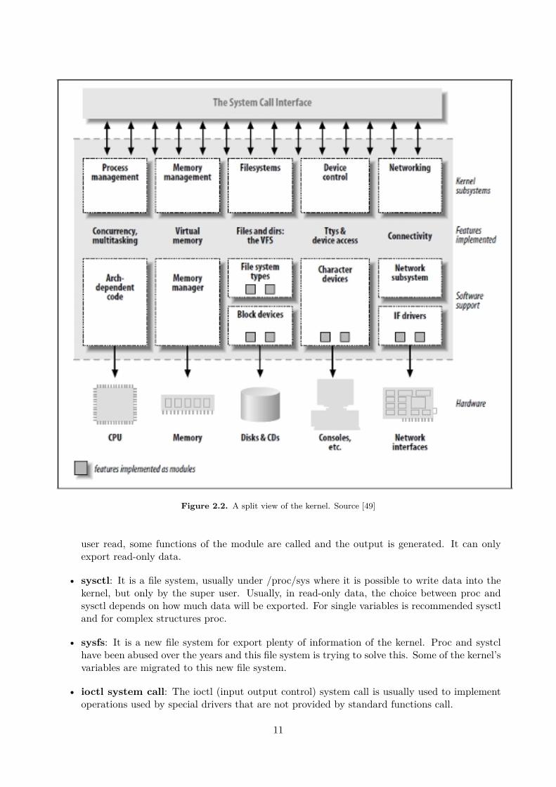
Figure 2.2. A split view of the kernel. Source [49]

user read, some functions of the module are called and the output is generated. It can onlyexport read-only data.

• sysctl: It is a file system, usually under /proc/sys where it is possible to write data into thekernel, but only by the super user. Usually, in read-only data, the choice between proc andsysctl depends on how much data will be exported. For single variables is recommended sysctland for complex structures proc.

• sysfs: It is a new file system for export plenty of information of the kernel. Proc and systclhave been abused over the years and this file system is trying to solve this. Some of the kernel’svariables are migrated to this new file system.

• ioctl system call: The ioctl (input output control) system call is usually used to implementoperations used by special drivers that are not provided by standard functions call.

11

• Netlink: It is the newest interface with the kernel. It is used like a socket and allows commu-nicating directly with the kernel. It allows bidirectional communication but only in datagrammode.

2.2.3 Network subsystem

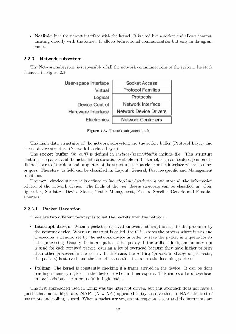
The Network subsystem is responsible of all the network communications of the system. Its stackis shown in Figure 2.3.

Figure 2.3. Network subsystem stack

The main data structures of the network subsystem are the socket buffer (Protocol Layer) andthe netdevice structure (Network Interface Layer).

The socket buffer (sk_buff) is defined in include/linux/skbuff.h include file. This structurecontains the packet and its meta-data associated available in the kernel, such as headers, pointers todifferent parts of the data and properties of the structure such as clone or the interface where it comesor goes. Therefore its field can be classified in: Layout, General, Feature-specific and Managementfunctions.

The net_device structure is defined in include/linux/netdevice.h and store all the informationrelated of the network device. The fields of the net_device structure can be classified in: Con-figuration, Statistics, Device Status, Traffic Management, Feature Specific, Generic and FunctionPointers.

2.2.3.1 Packet Reception

There are two different techniques to get the packets from the network:

• Interrupt driven. When a packet is received an event interrupt is sent to the processor bythe network device. When an interrupt is called, the CPU stores the process where it was andit executes a handler set by the network device in order to save the packet in a queue for itslater processing. Usually the interrupt has to be quickly. If the traffic is high, and an interruptis send for each received packet, causing a lot of overhead because they have higher prioritythan other processes in the kernel. In this case, the soft-irq (process in charge of processingthe packets) is starved, and the kernel has no time to process the incoming packets.

• Polling. The kernel is constantly checking if a frame arrived in the device. It can be donereading a memory register in the device or when a timer expires. This causes a lot of overheadin low loads but it can be useful in high loads.

The first approached used in Linux was the interrupt driven, but this approach does not have agood behaviour at high rate. NAPI (New API) appeared to try to solve this. In NAPI the best ofinterrupts and polling is used. When a packet arrives, an interruption is sent and the interrupts are

12

disabled. After processing all the incoming packets the interrupts are enabled again. Meanwhile if apacket arrives when another packet is processed, it is stored in the reception ring of the device butno interruption is sent. This technique improves the performance of the system at high rates. Also,the delay and performance problems of the interruptions are partially solved.

In Figure 2.4 it is shown the path of a packet in the kernel from when it is received to when it isdelivered to the protocol handler. When the packet arrives and receives the packet, the network driversends an interrupt to the service routine, which enqueue the device to the network soft interrupts.When the CPU attends the softirq, all devices that have been received packets are polled and then theinformation of the new packet is sent via the netif_receive_skb to the protocol handlers associatedwith the packet protocol.

Figure 2.4. Packet path in the reception. Source [50]

2.3 Pktgen studyThis section contains a study of the functions and the behaviour of Pktgen. This will be useful

in the future chapters in order to understand how it works and the modifications on it.

2.3.1 About

Pktgen is a packet generator which allows sending to the network preconfigured packets as fastas the system supports. It is freely available in almost all current Linux Kernels.

It is a very powerful tool to generate traffic in either PC, and allow testing network devices suchas router, switches, network drivers or network interfaces.

In order to increase its performance, it is implemented above the Linux Network drivers, whichinteracts with them with the API provided by the netdevice interface. Its idea is simple: push to the

13

NIC buffers as many packets as it can until they are full. Also enables to clone packets in order toreduce the time of creating and allocating new ones.

The latest implementation (version 2.73) has the following features:

• Support for MPLS, VLAN, IPSEC headers.

• Support for IP version 4 and 6.

• Customized the packets with multiples addresses

• Clone packets to improve performance

• Multi queue is implemented in the transmission. Different flows can be sent in the same interfacefrom different queues.

• Control and show the results via the proc file systems.

• Control the delay between packets.

• It uses UDP application protocol to send its own information. The discard port is used in orderthat the IP layer discards the packet in the reception.

The application layer contains the following 4-byte fields (16 Bytes in total) which are:

• pgh_magic: packet identifier that belong to a Pktgen transmission.

• seq_num: sequence number of the packet. If the packets are clone, there are gaps in thenumbering. The gaps have the size of the clone parameter.

• tv_sec: First part of the timestamp. The timestamp indicates when the packet is generated.

• tv_usec: Second part of the timestamp.

2.3.2 Pktgen Control and visualization

The control and the visualization of the results are implemented in three different proc file systems.

• pgcrtl: it is in charge of controlling the threads of Pktgen in order to start, stop or reset thetests.

• Pktgen_if : it is in charge of displaying the results and setting the parameters to the desiredinterface. The parameters available to change are: min_pkt_size, max_pkt_size, pkt_size,debug, frags, delay, udp_src_min, udp_dst_min, udp_src_max, udp_dst_max, clone_skb,count, src_mac_count, dst_mac_count, flag, dst_min, dst_max, dst6, dst6_min, dst6_max,src6, src_min, src_max, dst_mac, src_mac, clear_counters, flows, flowlen, queue_map_min,queue_map_max, mpls, vlan_id, vlan_p, vlan_cfi, svlan_id, svlan_p, svlan_cfi, tos and traf-fic_class.

• Pktgen_thread: it is in charge of setting the correct interfaces into the threads. The availablecommands are: add_device and rem_device_all

14

2.3.3 Pktgen operationWhen the module is loaded (pg_init), Pktgen makes the following things:

• Creates the profs directory of Pktgen and pgctrl file.

• Register the module to receive the netdevice events.

• Creates a thread for each CPU and attached to it, which it will be the function Pktgen_thread_worker.Also a procfs for each thread is created. This thread will be in charge of sending the packetsto the network interface.

When all the initializations and configuration via the procfs are done and the user sets start topgcrtl, the control is changed to RUN in order to start the transmission. When RUN is set to thethread, the initial packet and the output device (odev) are initialized via the function Pktgen_run().

The main flow of the thread worker is showed in Figure 2.5. In each loop an instance of thestruct pkt_dev is obtained by the function next_to_run(). This struct is used in the function forsending packets which is Pktgen_xmit(). Also there are functions for stopping the transmission(Pktgen_stop()), removing all the interfaces from the thread (Pktgen_rem_all_ifs()) or removingonly a specific interface (Pktgen_rem_one_if()). After each execution of the control functions, thecontrol flags are reversed.

Pktgen_xmit() is the function in charge of sending the correct packets. Its flow graph is showedin Figure 2.6. First of all, the device is checked in order to know if there is link and it is running.Otherwise, the device is stopped with the Pktgen_stop_function(). After that, the delay is checked.Then, it is checked if there is not a previous packet or there are not more clones of packets to do. Inthis case, a new packet is generated.

If the user has configured some delay and the last packet was transmitted OK, the program waitsfor the next transmission, otherwise continue with the transmission. There are two different waitingbehaviours which are implemented in the waiting function called spin. One is active (checking thecondition in a loop) and the other is freeing the CPU and scheduling the task in the future (in thecase of bigger waiting times). Once this is done, it is time to get the transmission queue from thenetdevice and block it.

Then if it is not stopped or frozen, the packet is send with the xmit function, and some variablesare updated depending on the result of the transmission. Finally, the transmission queue is unblocked.The last check is if the transmitted packets are the same or more than the expected packets to besend. In it is true, the device is stopped with the function Pktgen_stop_function().

15

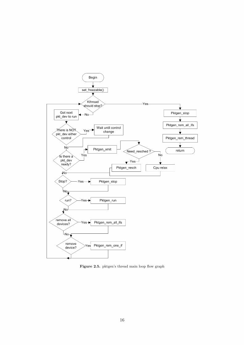
Figure 2.5. pktgen’s thread main loop flow graph

16

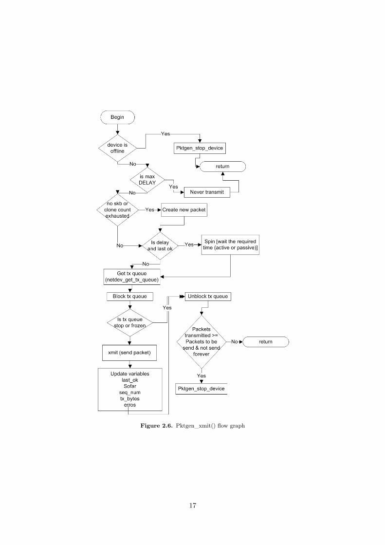
Figure 2.6. Pktgen_xmit() flow graph

17

Chapter 3

Design

This chapter contains the requirements and the design of the traffic analyzer implemented withpktgen. The design includes the architecture, the receiver metrics and the application interface. Alsoa overview of the operation is presented.

3.1 RequirementsThe goal of this project is to implement an open-source software to analyze high speed networks.

This software is based on pktgen module. The receiver modules is able to measure at high speed thebasic parameters used in benchmarking tools. The parameters are:

• Num of packets / Bytes received from the transmitter.

• Num of packets / Bytes lost in the network or element under test.

• Percentage of packets / Bytes lost.

• Throughput received from the link. Also the output throughput of pktgen will be adjustableby the user.

• Latency between transmitter and receiver.

• Inter-arrival time

• Jitter

The only action that the user needs to do is enabling the reception and the desired statistics.A private protocol for allowing the auto-configuration of the receiver is designed. Basically theapplication tells to the receiver part, which parameters will be used in the test.

The data collected is processed on real-time because in high traffics it is not possible to save allthe meta-data of the packets in memory and keep a high performance.

The receiver only process the packets coming from a pktgen packets generator.It takes advantage of the multi-queue network devices in multi-core systems, if they are available.

3.1.1 Not used parametersSome parameters used in different network analyzer tools that where studied in Chapter 2 or

defined in standards are discarded in the final design of the module for several reasons.The inter packet gap (Back to back frame, according with RFC 1242 [38]) is discarded because

there is not direct way to know it. The kernel only can stamp the time after receiving the packet.

19

Also, there is some delay between when the packet is received and it is delivered to the kernel. Alsodue to interrupt mitigation, some packets will be processed together and will have the same time.Moreover, an estimation of the transmission time is needed because it is not known at kernel levelwhen the NIC starts to receive the packet. Nowadays, only specialized hardware solutions are ableto get this type of statistics.

TCP statistics are also exclude because pktgen does not use TCP stack to send the packets. Alsoout of order packets, CRC checks are excluded. Moreover advance traffic generator and analyzingdistributions are excluded.

3.2 Architecture

In order to increase the performance, the sender and the receiver should be in different machines.Also, in order to reduce the time for getting the counter, each CPU has independent counters forthe received packets. Different reception formats could be used without modification the code. Inorder to work properly, each network queue interrupt should be attached to a different processor.Multi-queue reception is available in the Linux Kernel since version 2.6.27.

There is one exception in the scenarios, which is when the latency is calculated. In this case,sender and receiver should be in the same machine. This gives a big advantage on measuring latency,because there are not problems of synchronization. At least two CPU are recommended becausepktgen consumes all the resources of one CPU when it sends packets at high speed.

The receiver part is attached to the system at Level 3, just above the device driver. It is at thesame level as IP. Both stacks receive the IP packets. In this way, the traffic on the network is notaffected. Also it is transparent to the user. On the other hand, it has more overload because the IPstack process the incoming packet. Pktgen usually uses UDP packets with discard port, so when thepacket arrives at UDP level, it is discarded.

3.3 Receiver metrics

This section describes how the data is processed to obtain the requirements.

3.3.1 Metrics computation

Num of packets and bytes received The variables containing the results of these two parametersincrement its value in every reception of a packet. The bytes received do not include the CRC bytes(4bytes). This is done for legacy compatibility. The pktgen sender do not compute these bytes whenit sends.

Num of packets / Bytes lost When the results are going to be displayed a subtract betweenthe expected packets and the received packets is done. The expected packets are obtained with aconfiguration protocol which is explained in Section 3.5.1.1.

Percentage of packets / Bytes lost When the results are going to display a division betweenthe packets or bytes lost and the packets or bytes expected is done.

Throughput received When the first packet is received (when the counter of received packetsis 0), the time is saved in a local variable. The time stamp for the last packet is update in eachreception due to the possibility of losses in the last packets. Then the throughput is calculated when

20

the results are going to be displayed with Equation 3.2 and Equation 3.1.

Throughput = packets receivedend time − start time (pps) (3.1)

Throughput = bytes received × 8end time − start time (bps) (3.2)

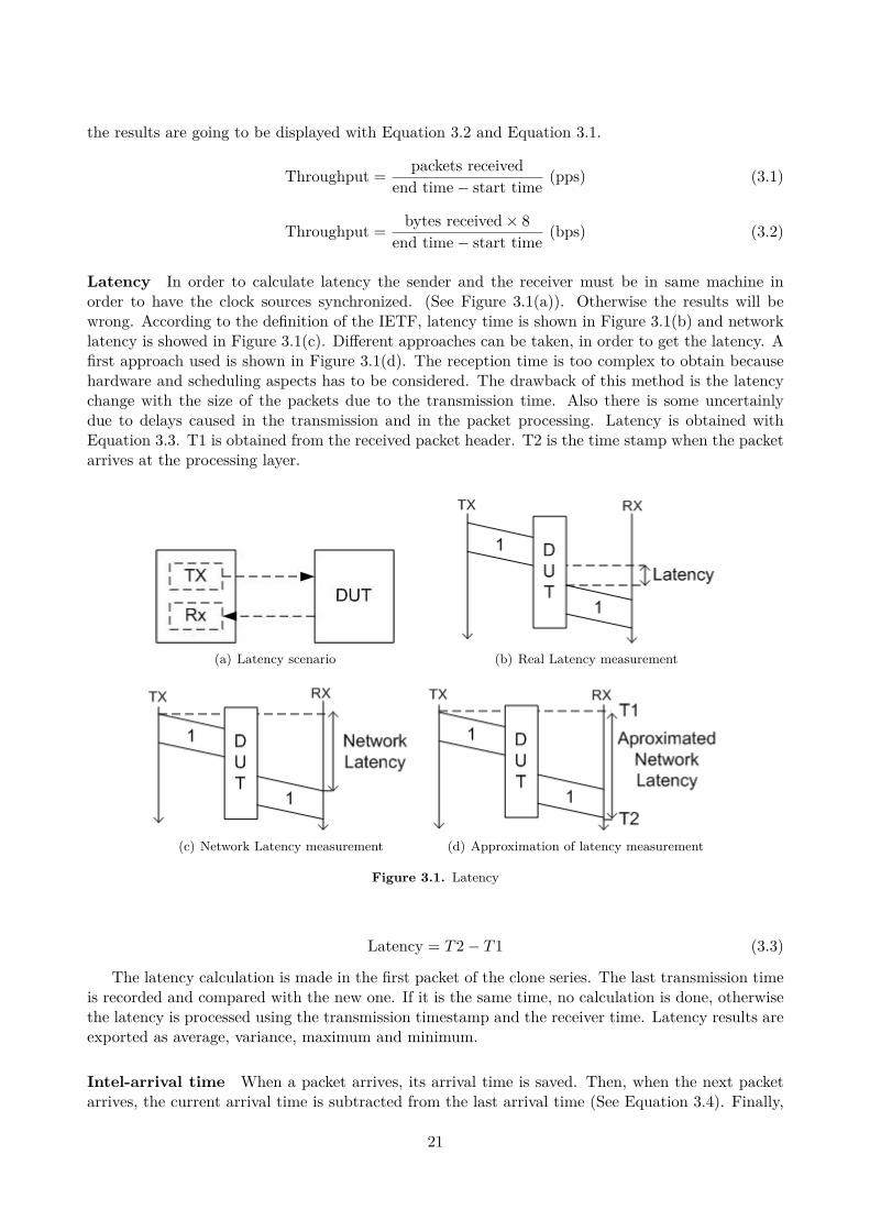
Latency In order to calculate latency the sender and the receiver must be in same machine inorder to have the clock sources synchronized. (See Figure 3.1(a)). Otherwise the results will bewrong. According to the definition of the IETF, latency time is shown in Figure 3.1(b) and networklatency is showed in Figure 3.1(c). Different approaches can be taken, in order to get the latency. Afirst approach used is shown in Figure 3.1(d). The reception time is too complex to obtain becausehardware and scheduling aspects has to be considered. The drawback of this method is the latencychange with the size of the packets due to the transmission time. Also there is some uncertainlydue to delays caused in the transmission and in the packet processing. Latency is obtained withEquation 3.3. T1 is obtained from the received packet header. T2 is the time stamp when the packetarrives at the processing layer.

(a) Latency scenario (b) Real Latency measurement

(c) Network Latency measurement (d) Approximation of latency measurement

Figure 3.1. Latency

Latency = T2 − T1 (3.3)

The latency calculation is made in the first packet of the clone series. The last transmission timeis recorded and compared with the new one. If it is the same time, no calculation is done, otherwisethe latency is processed using the transmission timestamp and the receiver time. Latency results areexported as average, variance, maximum and minimum.

Intel-arrival time When a packet arrives, its arrival time is saved. Then, when the next packetarrives, the current arrival time is subtracted from the last arrival time (See Equation 3.4). Finally,

21

the last packet arrival is saved. Then the results are exported as average, variance, maximum andminimum.

Inter arrival time = Tcurrent − Tlast arrival (3.4)

Jitter In order to calculate jitter, the inter-arrival method is used(See Section 2.1.5.2). Sending ina constant rate is necessary, otherwise the results will be wrong and it will depend on the transmitter.In this case, the last inter-arrival time calculated is required. It is assumed that pktgen sends atconstant rate. Jitter results are exported as average, variance, maximum and minimum.

3.3.2 Data collectionThe timestamp is extracted from the system, when it is needed. The high-resolution timer API

will be used to get the times in transmission and in the reception. The transmission timestamp isextracted from the packet headers.

The length of the packet is extracted from the socket buffer (skb) structure.

3.4 Application interfaceThe modification of pktgen uses proc file system in order to maintain backward compatibility.

Both user control and measurement visualization will be implemented in proc file system.

3.4.1 User ControlThe user control allows enabling the reception of packets and selecting the type and the format

of the statistics generated. The user interface is in a new file called /proc/net/pktgen/pgrx. Therequired data for generating the results is obtained with a configuration protocol and the receivermodule.

The added commands are:

• rx [device]: command that reset the counters and enable the reception of new packets. If thedevice name is not valid, all the interfaces will process their input packets.

• statistics [counters, basic or time]: command for selecting the statistics. Counter statis-tics includes those one that the time is not required (packets received, bytes received, packetslost, bytes lost). Basic statistics adds the receiver throughput. Time statistics additionallyincludes statistics that need more overload of the reception of the CPU because their process(inter-packet arrival time, latency and jitter). The default value is basic.

• rx_disable: command for stopping the receiver side of pktgen.

• rx_reset: command for resetting the values of the receiver.

• display [human, script]. Two different ways of displaying the results. See Subsection 3.4.2and 4.3.

3.4.2 Measurement visualizationThe results are displayed in a new file called /proc/net/pktgen/pgrx. It shows the receiver interface

and the parameters defined in Section 3.1. Two different formats are used to display the results. Thefirst one is for human reading and the second one for script reading.

The results are displayed per different CPU and then they are summarized for all the CPUs.

22

3.5 OperationThis section describes the operation of the main features of the modified pktgen.

3.5.1 Initialization

Pktgen can be controlled with a script which is in charge of passing the desired options to thekernel module. When the script calls start the test is initialized. The first packet is the configurationpacket. Then after waiting a predefined time (in order that the receiver process the configuration),the bulk transmission is initialized.

3.5.1.1 Configuration protocol

The minimum size of an Ethernet frame is 64 Bytes. The available free space header in thecurrent pktgen for inserting data is 64 - Ethernet Header (14 Bytes) - Ethernet CRC (4 Bytes)- IPHeader (20 Bytes) - UDP Header (8 Bytes) - PKTGEN Header (16 Bytes) = 2 Bytes. This spaceis not enough for sending the configuration to the receiver side during the test, so it is necessary tosend it before or after the test. It is necessary to create a new packet. The new header contains:

• Magic number (4 bytes). This field identifies a pktgen packet.

• Sequence number (4 bytes)

• Payload (Remaining space. Min 10 bytes)

The first packet (sequence number 0) sent is the configuration and it is not computed in thestatistics. The configuration header includes in the payload area:

• Packets to send (8 bytes). If it is 0 means infinite, so the statistics on the receiver side do notknow how many packets are transmitted. The sequence number is not a reliable source becauseit can have hops due to the clone skb parameter.

• Packet size (4 bytes)

The other packets on the payload will contain the timestamp when the packet is generated.

3.5.2 Packet transmission

The transmission mechanism available in the current pktgen module is used. Only some modifi-cations are done, such as the packet header and the throughput adjustment. There are two differentalternatives for generating a desired throughput: adjusting the delay between packets or sending afixed number of packets in a given interval.

On one hand, the first approach obtains a constant bit rate (CBR) traffic but it requires highaccuracy on high speed networks because the distance between packets is very small (ns). The gapbetween packets can be obtained with Equation 3.5, where P is the packet length of the packet inbits, Rt is the target throughput in bits per second and Lr is the link rate in bits per second. Also itis possible to calculate the interval between transmission packets, which required less resolution andit is shown in Equation 3.6.

gap delay(s) = P

Rt× (1 − Rt

Lr) (3.5)

transmission delay(s) = P

Rt(3.6)

23

On the other hand, the second approach does not required high time accuracy but it generates burstytraffic. It consists on calculating how many packets must be sent to get a target throughput. Whenall the packets are sent in a period, the transmitter wait until the next interval, where the counteris initialized again. The number of packets to send is shown in Equation 3.7, where Rt is the targetthroughput in b/s and Ti is the interval selected in seconds. In this case, it is not necessary to knowthe speed of the link.

packets in interval = Rt × Ti

Packet size (Bits) (3.7)

The first alternative is used.

3.5.3 Packet receptionThe program flow of the reception function depends on the statistics selected, which is selected

when the user sets the type of statistics. The structure of the function is the same for each type,but adding extra functionalities. The whole flow is shown in Figure 3.2. If the statistics is notrequired the block function in skipped. The timestamp of the system is disabled. The packets aretime stamped when being processed.

First, the read function checks if the received packet is a pktgen packet. If not, the packet isdrop. Then, if it sequence number is 0 (pktgen test sequence number usually starts at 1) it means itis a configuration packet, so the packets to send and the bytes to send is obtained. After that, thepacket is dropped because the configuration packet is not taken into account in the test.

The time is obtained when it is necessary to use it. Then, the inter-arrival time and the jitter iscalculated. When the process arrives to the latency part, the transmission time is checked. If it isdifferent than the previous one, it means that the packet is the first of a clone series. In this case,the latency is calculated. This allows to compute the latency during all the test.

In the throughput part, if the receiver packets variable is 0, the receiver gets the time stamp ofthe system and it is stored. Also, the last timestamp is saved as stop timestamp. Finally, the packetsreceived and the bytes received variables are updated.

24

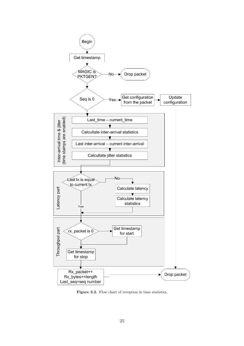
Figure 3.2. Flow chart of reception in time statistics.

25

Chapter 4

Implementation

This chapter includes some explanation of the implementation stage. Different steps were followedin order to obtain the code as optimized as possible. During the implementation stage, different testwere done in order to evaluate which is the best way to write the code. The tests had different initialconditions but their finality is to compare a specific implementation in order to see the gain or lossof performance. The final tests are explained in the next Chapter. The small packet size is usedbecause it requires more CPU resources.

This chapter explains different parts of the code and it justifies their election with some test.Also some concepts are introduced if they are necessary to understand the code.

4.1 Processing the incoming packet

Pktgen is modified in order to act as a L3 handler (sniffer) associated with IP packets and aspecific device (input_device). Also it is possible to capture from all the devices in the system. Atthis level, the compatibility with other modules and kernel functions is guaranteed. Also it is driverindependent and more generic. The drawback is that also IP has to process the packets. This canbe avoided modifying the network kernel subsystem (See Section 4.4), but then it is necessary torecompile the entire kernel.

When the incoming packets are processed, after allocating the socket buffer (skb), they are sentto the different protocols that want to process the packets. In order to add a receive handler it isnecessary to call the function (dev_add_pack()). This function need a parameter which is a packettype (Source 4.1). Basically it defines the handler function, the type of packets required and, alsoit is possible to specify the device (.dev). The handler is added when the user writes in the procfile system the option rx with the interface. If the interface is not valid, all the interfaces are used.The .dev field is changed in execution time in order to specify the correct listening device. Thisallows filtering the interface from where the traffic is processed. Also, the handler function is selectedaccording with the statistics selected (counter, basic or time).

stat ic struct packet_type pktgen_packet_type __read_mostly = {. type = __constant_htons (ETH_P_IP) ,. func = pktgen_rcv_basic ,. dev = NULL,

} ;

Source 4.1. struct pktgen_rx

27

4.1.1 Accessing data of the packetWhen a packet arrives, the first thing to do is checking if it is a pktgen packet. But before that,

it is necessary to obtain the pktgen header values from the packet. The packet data is stored inthe socket buffer structure (skb). The network card has two possible ways to store the packet data:linear and non linear.

In the linear way, the entire packet is in a continuous space of memory which allows to accessdirectly with an offset from the beginning of the packet. In the non-linear, the data is stored indifferent memory locations. The header is in the skb structure and the data is shared by all thereferences of the same packet and it is stored in pages.

A page is a structure of the kernel used to map different type of memory. The memory structureof the system is divided into different parts, usually protected between them. Mapping the packetdata in a page is usually done in the transmission side. For instance, the page points to the bufferdata of an UDP packet. This avoids copying the data from the user space buffer to the kernel spacebuffer. In this way, the data will be obtained directly from the original location and it will not bedifferent copies inside the system. Some cards also use this feature in the receiver side in order toreduce the number of packets’ copies. Then, both scenarios are possible and have to be taken intoaccount. The way how the information is stored depends on how to access it.

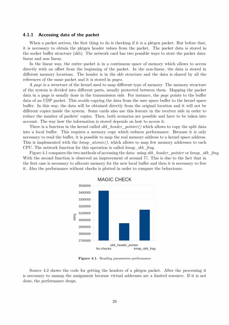
There is a function in the kernel called skb_header_pointer() which allows to copy the split datainto a local buffer. This requires a memory copy which reduces performance. Because it is onlynecessary to read the buffer, it is possible to map the real memory address to a kernel space address.This is implemented with the kmap_atomic(), which allows to map few memory addresses to eachCPU. The network function for this operation is called kmap_skb_frag.

Figure 4.1 compares the two methods of accessing the data: using skb_header_pointer or kmap_skb_frag.With the second function is observed an improvement of around 7�. This is due to the fact that inthe first case is necessary to allocate memory for the new local buffer and then it is necessary to freeit. Also the performance without checks is plotted in order to compare the behaviours.

No checksskb_header_pointer

kmap_skb_frag

2700000

2800000

2900000

3000000

3100000

3200000

3300000

3400000

3500000

MAGIC CHECK

PP

S

Figure 4.1. Reading parameters performance

Source 4.2 shows the code for getting the headers of a pktgen packet. After the processing itis necessary to unmap the assignment because virtual addresses are a limited resource. If it is notdone, the performance drops.

28

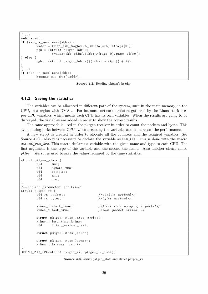
( . . . )void ∗vaddr ;i f ( skb_is_nonl inear ( skb ) ) {

vaddr = kmap_skb_frag(&skb_shinfo ( skb )−>f r a g s [ 0 ] ) ;pgh = ( struct pktgen_hdr ∗)

( vaddr+skb_shinfo ( skb )−>f r a g s [ 0 ] . page_of f s e t ) ;} else {

pgh = ( struct pktgen_hdr ∗) ( ( ( char ∗) ( iph ) ) + 28) ;}( . . . )i f ( skb_is_nonl inear ( skb ) )

kunmap_skb_frag ( vaddr ) ;

Source 4.2. Reading pktgen’s header

4.1.2 Saving the statistics

The variables can be allocated in different part of the system, such in the main memory, in theCPU, in a region with DMA ... For instance, network statistics gathered by the Linux stack usesper-CPU variables, which means each CPU has its own variables. When the results are going to bedisplayed, the variables are added in order to show the correct results.

The same approach is used in the pktgen receiver in order to count the packets and bytes. Thisavoids using locks between CPUs when accessing the variables and it increases the performance.

A new struct is created in order to allocate all the counters and the required variables (SeeSource 4.3). Also it is necessary to declare the variable as PER_CPU. This is done with the macroDEFINE_PER_CPU. This macro declares a variable with the given name and type to each CPU. Thefirst argument is the type of the variable and the second the name. Also another struct calledpktgen_stats it is used to save the values required by the time statistics.

struct pktgen_stats {u64 sum ;u64 square_sum ;u64 samples ;u64 min ;u64 max ;

} ;/∗ Receiver parameters per CPU∗/struct pktgen_rx {

u64 rx_packets ; /∗ packe t s a r r i v e d ∗/u64 rx_bytes ; /∗ b y t e s a r r i v e d ∗/

ktime_t start_time ; /∗ f i r s t time stamp o f a packe t ∗/ktime_t last_time ; /∗ l a s t packe t a r r i v a l ∗/

struct pktgen_stats i n t e r_a r r i v a l ;ktime_t last_time_ktime ;u64 i n t e r_a r r i v a l_ l a s t ;

struct pktgen_stats j i t t e r ;

struct pktgen_stats l a t ency ;ktime_t latency_last_tx ;

} ;DEFINE_PER_CPU( struct pktgen_rx , pktgen_rx_data ) ;

Source 4.3. struct pktgen_stats and struct pktgen_rx

29

There are two ways of accessing variables in a processor. If the variable is in the same processor,get_cpu_var is used. Otherwise, in order to access to the variable of a specific CPU, per_cpu isused. In Source 4.4 it is shown the two methods to access to the variables, concretely the packetsreceived counter.__get_cpu_var ( pktgen_rx_data ) . rx_packets++;per_cpu ( pktgen_rx_data , cpu ) . rx_packets ;

Source 4.4. Accessing data in per-CPU variable

4.1.3 Measuring timeThe time reference is only obtained once, in order to avoid overhead. Pktgen will use the clock

of the system obtained by ktime_get().Different approaches for getting the time stamp are evaluated. The first idea was to use the

network time stamps enabling it with the function net_enable_timestamp(), but this option wasdiscarded because the time resolution obtained was 1 millisecond.

The second option was using the Time Stamp Counter (TSC) clock. It is a 64 bit register presentin the x86 systems. There is a TSC clock for each CPU. The TSC clock increases its value ineach CPU cycle. The clock sources are not synchronized between the different CPUs. Also, if thedifferent CPUs have different frequency (due to the saving energy, especially on laptops) it will bedifferent increments for each CPU. Moreover, different types of processors increment the register indifferent ways. Read access to this clock is very fast, and in the current processors has a resolutionof nanoseconds. In the other hand, it’s architecture dependent.

The third option was using the hardware time stamps on the network card, but the accuracy wasnot good enough, because some packets had the same time, and others were not time stamped.

Because it is necessary a clock reference for the aggregated throughput of the different CPU,finally the TSC clock is discarded and the clock reference is provided by the kernel with the functionktime_get(). This functions gets the default clock of the system, which in the current scenario is aTSC clock of the 1st CPU. The available clocks can be listed with:

$cat /sys/devices/system/clocksource/clocksource0/available_clocksourcetsc hpet acpi_pm jiffies

After measuring the required parameters (inter-arrival time, jitter or latency), the data is pro-cessed and stored with the function in Source 4.5. Later, when the results are displayed, the currentvalue for the average and the variance is calculated.

The latency is only calculated when the transmitter and receiver is in the same machine. In thiscase, the packet is sent out in one interface and it is received in the other interface.void proce s s_s ta t s ( u64 value , struct pktgen_stats ∗ s t a t s ){

s ta t s−>square_sum += value ∗ value ;s t a t s−>sum += value ;

s t a t s−>samples++;

i f ( va lue > sta t s−>max)s ta t s−>max = value ;

i f ( va lue < sta t s−>min)s ta t s−>min = value ;

}

Source 4.5. Processing statistics

30

4.2 Auto-configuration of the receiverWhen the user adds the parameter config 1 (NEW parameter) the sender will send a configuration

packet. The legacy transmission system is modified to include the configuration data. Also a checkingin the receiver side is done in order to know if the arrived packet is a configuration packet or not.

4.2.1 SendingThe pktgen function fill_packet() is modified in order to include the config packet. The configu-

ration flag is only active before starting the transmission. When the flag is active, the configurationpacket is created. It is necessary to change the size of the allocate packet. Also a new packet structis created (See Source 4.6).struct pktgen_hdr_config {

__be32 pgh_magic ;__be32 seq_num ;__u64 pkt_to_send ;__be16 pkt_size ;

} ;

Source 4.6. struct pktgen_hdr_config

When the configuration flag is activated, after sending the first packet (config) the transmissionwaits a predefined time. This is done in order to give some time to the receiver to process theconfiguration packets and reset its counters. After that time, the configuration flag is set to 0, andthe starting time of the test is reset. Also, a packet is discounted from the packets sent. Doing that,the configuration packets do not have any effect in the test.

4.2.2 ReceiverThe receiver function checks for each packet if the sequence number is 0. It is possible to receive

more than one configuration packet in each test. This is due to the fact that a configuration packetis generated for each pktgen thread. When the first packet is received, the counters are reset andthe packets to send and the bytes to sent are set. In the next configuration packets, the values ofthe packets and bytes to send are updated. In order to know if it is a new test or the same one, thetime when the configuration packets are received is saved. If the difference between the arrivals isless that the configuration delay time, it is considered the same test, otherwise a different one. (SeeSource 4.7)stat ic int i s_conf igure_packet (void ∗header ){

struct pktgen_hdr ∗pgh = ( struct pktgen_hdr ∗) header ;

i f ( l i k e l y (pgh−>seq_num) != 0)return 0 ;

else {struct pktgen_hdr_config ∗pghc =

( struct pktgen_hdr_config ∗) header ;u64 pkts = ntohl ( pghc−>pkt_to_send ) ;int pkt_size = ntohs ( pghc−>pkt_size ) ;

u64 time_from_last ;ktime_t now ;

spin_lock (&(pg_rx_global−>conf ig_lock ) ) ;now = ktime_now ( ) ;time_from_last = ktime_to_us ( ktime_sub (now ,

31

pg_rx_global−>la s t_con f i g ) ) ;

i f ( time_from_last < TIME_CONFIG_US) {pg_rx_global−>pkts_to_send += pkts ;pg_rx_global−>bytes_to_send += pkt_size ∗pkts ;

} else {pg_reset_rx ( ) ;pg_rx_global−>pkts_to_send = pkts ;pg_rx_global−>bytes_to_send = pkt_size ∗pkts ;

}pg_rx_global−>la s t_con f i g = now ;spin_unlock (&(pg_rx_global−>conf ig_lock ) ) ;return 1 ;

}}

Source 4.7. Receiving configuration packet

4.3 Displaying the resultsThe results are displayed in the proc file system. Two type of visualization are possible: human

readable and script readable. Using the macro in Source 4.8 is it possible to display multiple formatswith only one call. In order to choose between both formats, it is necessary to write display humanor display script in the receiver proc file system. The default is text.#define DISPLAY_RX( opt , seq , fmt , fmt1 , args . . . ) \

i f ( opt == PG_DISPLAY_HUMAN) \seq_pr int f ( seq , fmt1 ,## args ) ; \

else \seq_pr int f ( seq , fmt ,## args ) ;

Source 4.8. Macro for displaying results

Two different statistics are displayed. First, there is the statistics per CPU, where the timestatistics are displayed if the option is enabled. Second, there is a summary of the test. If theconfiguration packet is sent, it also includes the expected packets and bytes and the losses. Thepercentage of losses is not possible to display because float operations are not allowed inside thekernel. The throughput is always displayed.

Source 4.9 is an example of a time reception statistics in a gigabit link. It is shown the detailsof each parameter measured. The latency appears only if the sender and receiver are in the samemachine.

RECEPTION STATISTICSPER−CPU Stat s

CPU 0 : Rx packets : 0 Rx bytes : 0CPU 1 : Rx packets : 0 Rx bytes : 0CPU 2 : Rx packets : 10000000 Rx bytes : 600000000

Work time 6719014 usRate : 1488313 pps 714Mb/ sec (714390534 bps )Inter−a r r i v a l

Average : 671 ns Variance 381245 ns2Max: 10108 ns Min : : 404 nsSamples : 9999999

J i t t e rAverage : 360 ns Variance 665018 ns2Max: 9404 ns Min : : 0 nsSamples : 9999998

Latency

32

Average : 470578 ns Variance 216731083 ns2Max: 545217 ns Min : : 60345 nsSamples : 1000000

CPU 3 : Rx packets : 0 Rx bytes : 0CPU 4 : Rx packets : 0 Rx bytes : 0CPU 5 : Rx packets : 0 Rx bytes : 0CPU 6 : Rx packets : 0 Rx bytes : 0CPU 7 : Rx packets : 0 Rx bytes : 0

Global S t a t i s t i c sPackets Rx : 10000000 Bytes Rx : 600000000Packets Ex : 10000000 Bytes Ex : 600000000Packets Lost : 0 Bytes Lost : 0

Work time 6719014 usRate : 1488313 pps 714Mb/ sec (714390534 bps )

Source 4.9. Time statistics in one CPU

Source 4.10 and Source 4.11 are examples of the human and script readable formats.

cat /proc /net /pktgen/pgrxRECEPTION STATISTICS

PER−CPU Stat sCPU 0 : Rx packets : 0 Rx bytes : 0CPU 1 : Rx packets : 0 Rx bytes : 0CPU 2 : Rx packets : 9385641 Rx bytes : 563138460

Work time 13483820 usRate : 696066 pps 334Mb/ sec (334112119 bps )

CPU 3 : Rx packets : 9490524 Rx bytes : 569431440Work time 13483381 usRate : 703868 pps 337Mb/ sec (337856767 bps )

CPU 4 : Rx packets : 8949667 Rx bytes : 536980020Work time 13483488 usRate : 663750 pps 318Mb/ sec (318600065 bps )

CPU 5 : Rx packets : 9030598 Rx bytes : 541835880Work time 13483509 usRate : 669751 pps 321Mb/ sec (321480635 bps )

CPU 6 : Rx packets : 9085660 Rx bytes : 545139600Work time 13483696 usRate : 673825 pps 323Mb/ sec (323436304 bps )

CPU 7 : Rx packets : 9009976 Rx bytes : 540598560Work time 13483359 usRate : 668229 pps 320Mb/ sec (320750080 bps )

Global S t a t i s t i c sPackets Rx : 54952066 Bytes Rx : 3297123960Work time 13483828 us4075405 pps 1956Mb/ sec (1956194611 bps )

Source 4.10. Displaying human readable

# cat /proc /net /pktgen/pgrx0 0 0 0 0 01 0 0 0 0 02 9569752 574185120 13667949 700160 336 3360768293 9591125 575467500 13667867 701728 336 3368294404 9109725 546583500 13667629 666518 319 3199287895 9159094 549545640 13668004 670112 321 3216537776 9163423 549805380 13667956 670431 321 3218069357 9123356 547401360 13667953 667499 320 320399907G 55716475 3342988500 13668064 4076398 1956 1956671259

33

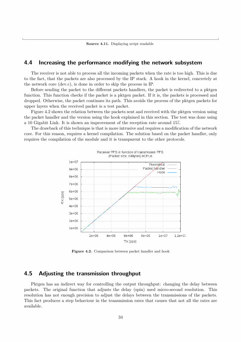
Source 4.11. Displaying script readable

4.4 Increasing the performance modifying the network subsystemThe receiver is not able to process all the incoming packets when the rate is too high. This is due

to the fact, that the packets are also processed by the IP stack. A hook in the kernel, concretely atthe network core (dev.c), is done in order to skip the process in IP.

Before sending the packet to the different packets handlers, the packet is redirected to a pktgenfunction. This function checks if the packet is a pktgen packet. If it is, the packets is processed anddropped. Otherwise, the packet continues its path. This avoids the process of the pktgen packets forupper layers when the received packet is a test packet.

Figure 4.2 shows the relation between the packets sent and received with the pktgen version usingthe packet handler and the version using the hook explained in this section. The test was done usinga 10 Gigabit Link. It is shown an improvement of the reception rate around 15�.

The drawback of this technique is that is more intrusive and requires a modification of the networkcore. For this reason, requires a kernel compilation. The solution based on the packet handler, onlyrequires the compilation of the module and it is transparent to the other protocols.

Figure 4.2. Comparison between packet handler and hook

4.5 Adjusting the transmission throughputPktgen has an indirect way for controlling the output throughput: changing the delay between

packets. The original function that adjusts the delay (spin) used micro-second resolution. Thisresolution has not enough precision to adjust the delays between the transmissions of the packets.This fact produces a step behaviour in the transmission rates that causes that not all the rates areavailable.

34

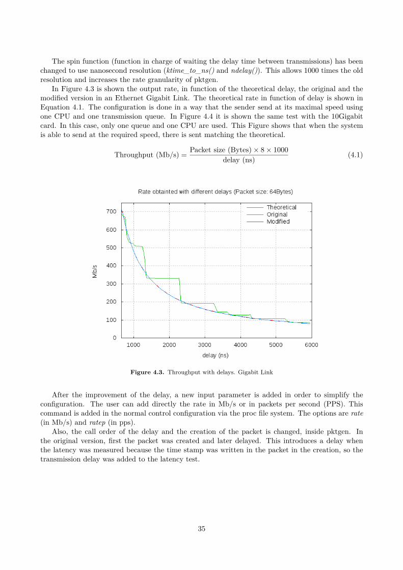
The spin function (function in charge of waiting the delay time between transmissions) has beenchanged to use nanosecond resolution (ktime_to_ns() and ndelay()). This allows 1000 times the oldresolution and increases the rate granularity of pktgen.

In Figure 4.3 is shown the output rate, in function of the theoretical delay, the original and themodified version in an Ethernet Gigabit Link. The theoretical rate in function of delay is shown inEquation 4.1. The configuration is done in a way that the sender send at its maximal speed usingone CPU and one transmission queue. In Figure 4.4 it is shown the same test with the 10Gigabitcard. In this case, only one queue and one CPU are used. This Figure shows that when the systemis able to send at the required speed, there is sent matching the theoretical.

Throughput (Mb/s) = Packet size (Bytes) × 8 × 1000delay (ns) (4.1)

Figure 4.3. Throughput with delays. Gigabit Link

After the improvement of the delay, a new input parameter is added in order to simplify theconfiguration. The user can add directly the rate in Mb/s or in packets per second (PPS). Thiscommand is added in the normal control configuration via the proc file system. The options are rate(in Mb/s) and ratep (in pps).

Also, the call order of the delay and the creation of the packet is changed, inside pktgen. Inthe original version, first the packet was created and later delayed. This introduces a delay whenthe latency was measured because the time stamp was written in the packet in the creation, so thetransmission delay was added to the latency test.

35

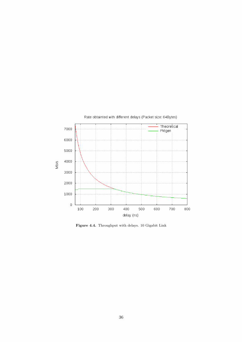
Figure 4.4. Throughput with delays. 10 Gigabit Link

36

Chapter 5

Evaluation

This chapter includes some test in order to calibrate the implementation. Because the receptionof the packets is directly related with the network subsystem, also the behaviour of the Linux receiveris shown. Moreover, additional tests related with the performance are done.

5.1 Equipment and scenarioThere are two machines with the characteristics described in the next subsections. Different

scenarios were used in order to do the test.

5.1.1 Hardware

The motherboard is a TYAN S7002. The processors of the test machine are: Intel(R) Xeon(R)CPU E5520 at 2.27GHz. It is a Quad-Core processor with Hyperthreading [51], which in practicegives 8 available CPUs. The system has 3 Gigabyte (3x1Gigabyte) of DDR3 (1333MHz) RAM.

The available network cards on the system are:

• 2 Intel 82574L Gigabit Network (2 built in Copper Port): eth0, eth1

• 4 Intel 82576 Gigabit Network (2 x Dual Copper Port): eth2, eth3, eth4, eth5

• 2 Intel 82599EB 10-Gigabit Network (1 x Dual Fibre Port): eth6, eth7

There are two test machines available (host1 and host2).

5.1.2 Software

The operating system running on the test machines is Linux with Bifrost Distribution [52]. Thekernel was obtained from net-next repository [53] in the 8th April of 2010. The version is 2.6.34-rc2.

Bifrost distribution is a Linux distribution focus on networking. It is used in open source routers.Net-next repository is the kernel development repository where are the latest features for the networksubsystem. It runs on a USB memory stick.

5.1.3 Scenarios

Different scenarios were tested in order to evaluate the different features introduced in the pktgenmodification. Almost all the tests were done with a direct connection between the two hosts. Thisavoids any interference between sender and receiver, and it allows higher rates in the 10 Gigabitenvironments. The only exception was the latency test, where a local loop between the interfaces

37

was done. In the Gigabit environment, two different physical cards were used. In the 10 Gigabitenvironments, one CPU is used for sending, and two for receiving. Table 5.1 shows the interfacesused in the tested scenarios.

Scenario Name TX interface (Host) RX interface (Host) SpeedA eth7 (host1) eth7 (host2) 10GB eth4 (host1) eth4 (host2) 1GC eth5 (host2) eth3 (host2) 1GD eth6 (host2) eth7 (host2) 10G

Table 5.1. Test scenarios

5.1.4 Parameters under study

Several parameters were monitored in order to evaluate the system.

• Throughput received: the units are in packets per second. The maximal theoretical number ofpackets per second in Gigabit links is 1,48 Mpps and for the 10 Gigabit links is 14,8Mpps. Thisvalue is obtained with the minimal Ethernet packet size (64 Bytes) plus the Ethernet preamble(14 bytes) and the inter packet gap (6 bytes).

• Time statistics: the results of the defined parameters in the previous chapters. They areexpressed in nanoseconds.

• Interrupts: number of interrupt per second caused by the network device. This can help tounderstand some of the behaviours.

5.2 Validation and CalibrationThis section includes the test of the received throughput with different CPUs and the validation

and calibration of the different statistics collected by the pktgen module.

5.2.1 Receiver throughput

The maximal received throughput was tested. Scenario A and B were used, but the main interestis focus on scenario A because of the higher rates.

First, how much traffic was able to send the transmitter with the 10G card with the small packetsize was tested. It was able to send up to 11,5 Mpps. In order to archive the maximal speed, it isnecessary to send at least with 4 CPUs. One CPU does not have enough processing power to createand sent all the packets. Nevertheless, the wire speed is not archived. This is a hardware limitationand is produced for architecture limitations, such as the bus capacity in terms on transaction persecond. The results are shown in Figure 5.1.

The receiver test was done changing the number of queues on the receiver. Each queue is attachedto different processors. Each CPU has to have the same number of queues, otherwise the load isnot balanced and their performance is reduced. The objective of this test is to check the amount oftraffic that the system is able to process using different queues and CPUs. Also different flows aresimulated because a single flow always goes to the same queue in order to avoid packet reordering.The parameters used by the pktgen sender are shown in Table 5.2.

The results of the test are plotted in Figure 5.2(a). It is shown that from 1 to 4, there isan increment of the maximal received throughput. With 5 CPUs there is a drop in the received

38

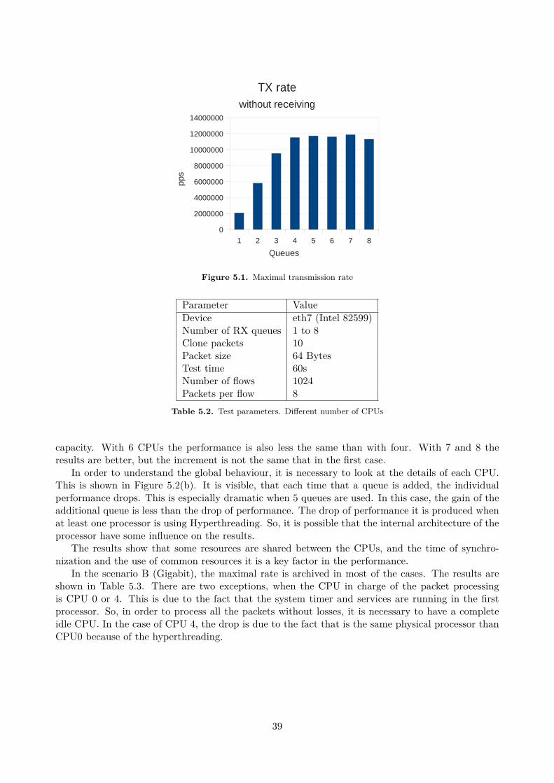
1 2 3 4 5 6 7 8

0

2000000

4000000

6000000

8000000

10000000

12000000

14000000

TX ratewithout receiving

Queues

pp

s

Figure 5.1. Maximal transmission rate

Parameter ValueDevice eth7 (Intel 82599)Number of RX queues 1 to 8Clone packets 10Packet size 64 BytesTest time 60sNumber of flows 1024Packets per flow 8

Table 5.2. Test parameters. Different number of CPUs

capacity. With 6 CPUs the performance is also less the same than with four. With 7 and 8 theresults are better, but the increment is not the same that in the first case.

In order to understand the global behaviour, it is necessary to look at the details of each CPU.This is shown in Figure 5.2(b). It is visible, that each time that a queue is added, the individualperformance drops. This is especially dramatic when 5 queues are used. In this case, the gain of theadditional queue is less than the drop of performance. The drop of performance it is produced whenat least one processor is using Hyperthreading. So, it is possible that the internal architecture of theprocessor have some influence on the results.

The results show that some resources are shared between the CPUs, and the time of synchro-nization and the use of common resources it is a key factor in the performance.

In the scenario B (Gigabit), the maximal rate is archived in most of the cases. The results areshown in Table 5.3. There are two exceptions, when the CPU in charge of the packet processingis CPU 0 or 4. This is due to the fact that the system timer and services are running in the firstprocessor. So, in order to process all the packets without losses, it is necessary to have a completeidle CPU. In the case of CPU 4, the drop is due to the fact that is the same physical processor thanCPU0 because of the hyperthreading.

39

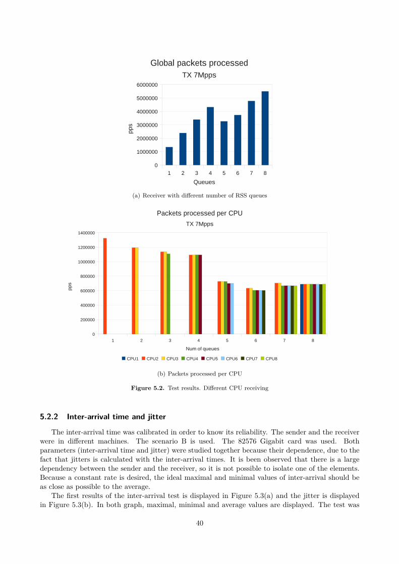
1 2 3 4 5 6 7 8

0

1000000

2000000

3000000

4000000

5000000

6000000

Global packets processedTX 7Mpps

Queues

pp

s

(a) Receiver with different number of RSS queues

1 2 3 4 5 6 7 8

0

200000

400000

600000

800000

1000000

1200000

1400000

Packets processed per CPU

TX 7Mpps

CPU1 CPU2 CPU3 CPU4 CPU5 CPU6 CPU7 CPU8

Num of queues

pp

s

(b) Packets processed per CPU

Figure 5.2. Test results. Different CPU receiving

5.2.2 Inter-arrival time and jitter

The inter-arrival time was calibrated in order to know its reliability. The sender and the receiverwere in different machines. The scenario B is used. The 82576 Gigabit card was used. Bothparameters (inter-arrival time and jitter) were studied together because their dependence, due to thefact that jitters is calculated with the inter-arrival times. It is been observed that there is a largedependency between the sender and the receiver, so it is not possible to isolate one of the elements.Because a constant rate is desired, the ideal maximal and minimal values of inter-arrival should beas close as possible to the average.

The first results of the inter-arrival test is displayed in Figure 5.3(a) and the jitter is displayedin Figure 5.3(b). In both graph, maximal, minimal and average values are displayed. The test was

40

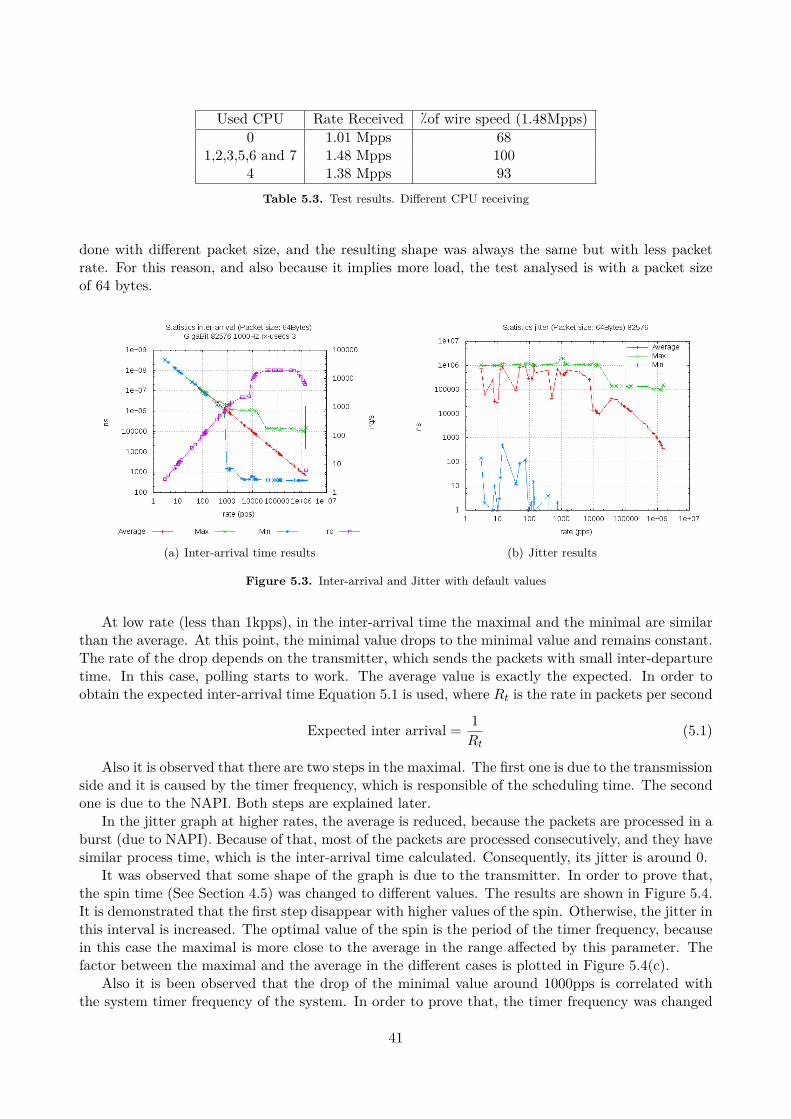
Used CPU Rate Received �of wire speed (1.48Mpps)0 1.01 Mpps 68

1,2,3,5,6 and 7 1.48 Mpps 1004 1.38 Mpps 93

Table 5.3. Test results. Different CPU receiving

done with different packet size, and the resulting shape was always the same but with less packetrate. For this reason, and also because it implies more load, the test analysed is with a packet sizeof 64 bytes.

(a) Inter-arrival time results (b) Jitter results

Figure 5.3. Inter-arrival and Jitter with default values

At low rate (less than 1kpps), in the inter-arrival time the maximal and the minimal are similarthan the average. At this point, the minimal value drops to the minimal value and remains constant.The rate of the drop depends on the transmitter, which sends the packets with small inter-departuretime. In this case, polling starts to work. The average value is exactly the expected. In order toobtain the expected inter-arrival time Equation 5.1 is used, where Rt is the rate in packets per second

Expected inter arrival = 1Rt

(5.1)

Also it is observed that there are two steps in the maximal. The first one is due to the transmissionside and it is caused by the timer frequency, which is responsible of the scheduling time. The secondone is due to the NAPI. Both steps are explained later.

In the jitter graph at higher rates, the average is reduced, because the packets are processed in aburst (due to NAPI). Because of that, most of the packets are processed consecutively, and they havesimilar process time, which is the inter-arrival time calculated. Consequently, its jitter is around 0.

It was observed that some shape of the graph is due to the transmitter. In order to prove that,the spin time (See Section 4.5) was changed to different values. The results are shown in Figure 5.4.It is demonstrated that the first step disappear with higher values of the spin. Otherwise, the jitter inthis interval is increased. The optimal value of the spin is the period of the timer frequency, becausein this case the maximal is more close to the average in the range affected by this parameter. Thefactor between the maximal and the average in the different cases is plotted in Figure 5.4(c).

Also it is been observed that the drop of the minimal value around 1000pps is correlated withthe system timer frequency of the system. In order to prove that, the timer frequency was changed

41

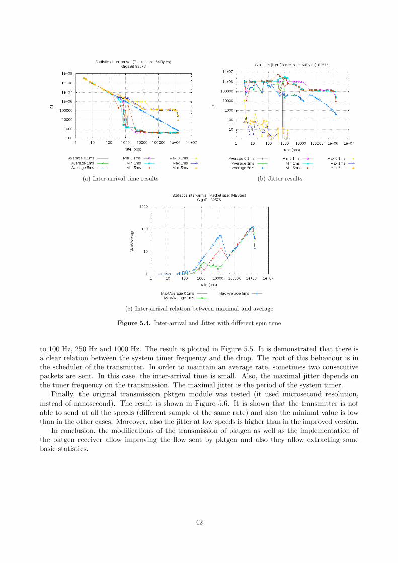
(a) Inter-arrival time results (b) Jitter results

(c) Inter-arrival relation between maximal and average

Figure 5.4. Inter-arrival and Jitter with different spin time

to 100 Hz, 250 Hz and 1000 Hz. The result is plotted in Figure 5.5. It is demonstrated that there isa clear relation between the system timer frequency and the drop. The root of this behaviour is inthe scheduler of the transmitter. In order to maintain an average rate, sometimes two consecutivepackets are sent. In this case, the inter-arrival time is small. Also, the maximal jitter depends onthe timer frequency on the transmission. The maximal jitter is the period of the system timer.

Finally, the original transmission pktgen module was tested (it used microsecond resolution,instead of nanosecond). The result is shown in Figure 5.6. It is shown that the transmitter is notable to send at all the speeds (different sample of the same rate) and also the minimal value is lowthan in the other cases. Moreover, also the jitter at low speeds is higher than in the improved version.

In conclusion, the modifications of the transmission of pktgen as well as the implementation ofthe pktgen receiver allow improving the flow sent by pktgen and also they allow extracting somebasic statistics.

42

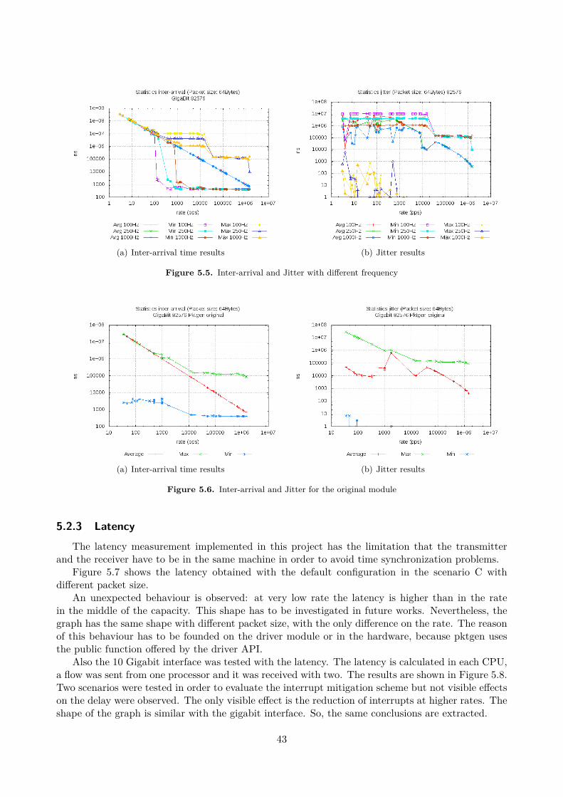
(a) Inter-arrival time results (b) Jitter results

Figure 5.5. Inter-arrival and Jitter with different frequency

(a) Inter-arrival time results (b) Jitter results

Figure 5.6. Inter-arrival and Jitter for the original module

5.2.3 Latency

The latency measurement implemented in this project has the limitation that the transmitterand the receiver have to be in the same machine in order to avoid time synchronization problems.

Figure 5.7 shows the latency obtained with the default configuration in the scenario C withdifferent packet size.

An unexpected behaviour is observed: at very low rate the latency is higher than in the ratein the middle of the capacity. This shape has to be investigated in future works. Nevertheless, thegraph has the same shape with different packet size, with the only difference on the rate. The reasonof this behaviour has to be founded on the driver module or in the hardware, because pktgen usesthe public function offered by the driver API.

Also the 10 Gigabit interface was tested with the latency. The latency is calculated in each CPU,a flow was sent from one processor and it was received with two. The results are shown in Figure 5.8.Two scenarios were tested in order to evaluate the interrupt mitigation scheme but not visible effectson the delay were observed. The only visible effect is the reduction of interrupts at higher rates. Theshape of the graph is similar with the gigabit interface. So, the same conclusions are extracted.

43

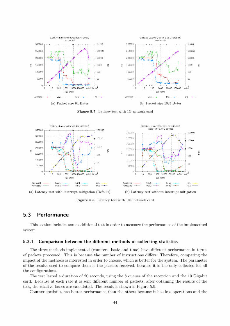
(a) Packet size 64 Bytes (b) Packet size 1024 Bytes

Figure 5.7. Latency test with 1G network card

(a) Latency test with interrupt mitigation (Default) (b) Latency test without interrupt mitigation

Figure 5.8. Latency test with 10G network card

5.3 PerformanceThis section includes some additional test in order to measure the performance of the implemented

system.

5.3.1 Comparison between the different methods of collecting statisticsThe three methods implemented (counters, basic and time) have different performance in terms

of packets processed. This is because the number of instructions differs. Therefore, comparing theimpact of the methods is interested in order to choose, which is better for the system. The parameterof the results used to compare them is the packets received, because it is the only collected for allthe configurations.

The test lasted a duration of 20 seconds, using the 8 queues of the reception and the 10 Gigabitcard. Because at each rate it is sent different number of packets, after obtaining the results of thetest, the relative losses are calculated. The result is shown is Figure 5.9.

Counter statistics has better performance than the others because it has less operations and the

44

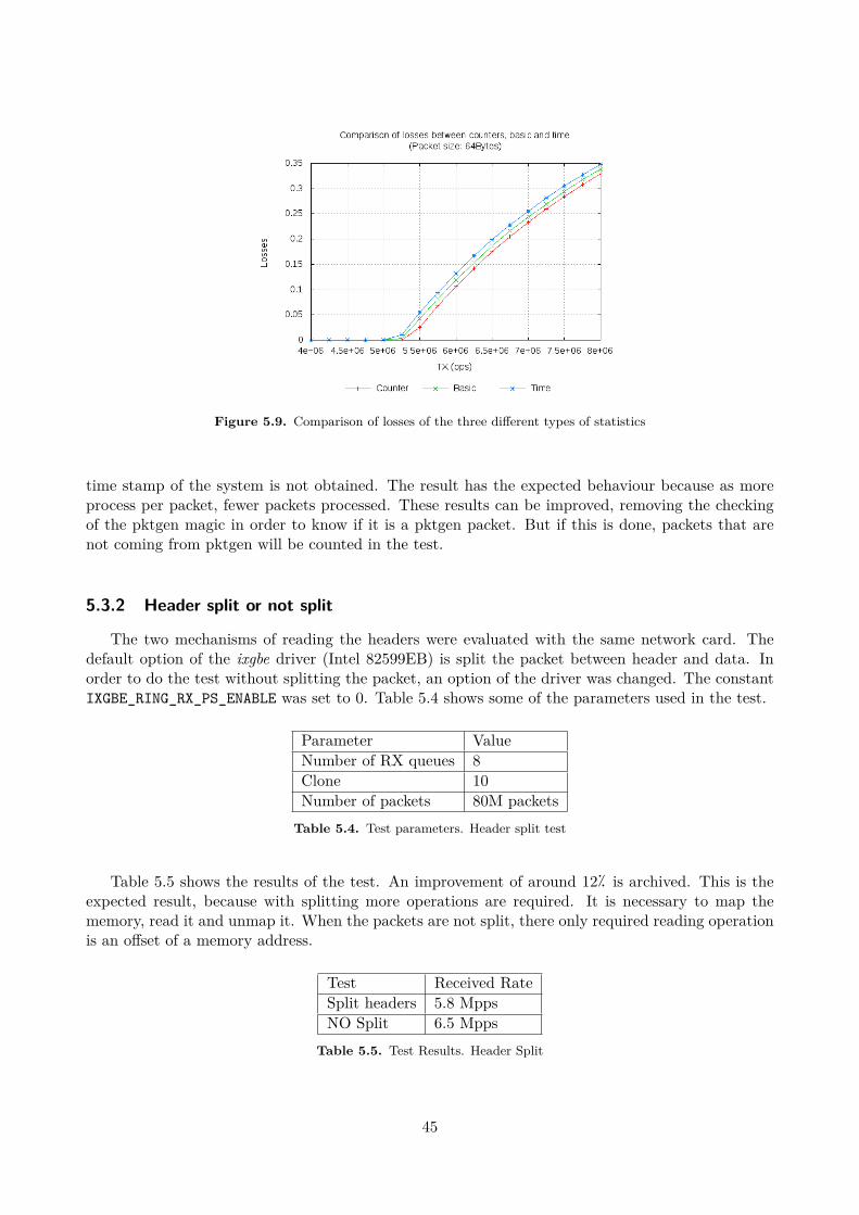
Figure 5.9. Comparison of losses of the three different types of statistics

time stamp of the system is not obtained. The result has the expected behaviour because as moreprocess per packet, fewer packets processed. These results can be improved, removing the checkingof the pktgen magic in order to know if it is a pktgen packet. But if this is done, packets that arenot coming from pktgen will be counted in the test.

5.3.2 Header split or not split

The two mechanisms of reading the headers were evaluated with the same network card. Thedefault option of the ixgbe driver (Intel 82599EB) is split the packet between header and data. Inorder to do the test without splitting the packet, an option of the driver was changed. The constantIXGBE_RING_RX_PS_ENABLE was set to 0. Table 5.4 shows some of the parameters used in the test.

Parameter ValueNumber of RX queues 8Clone 10Number of packets 80M packets

Table 5.4. Test parameters. Header split test

Table 5.5 shows the results of the test. An improvement of around 12� is archived. This is theexpected result, because with splitting more operations are required. It is necessary to map thememory, read it and unmap it. When the packets are not split, there only required reading operationis an offset of a memory address.

Test Received RateSplit headers 5.8 MppsNO Split 6.5 Mpps

Table 5.5. Test Results. Header Split

45

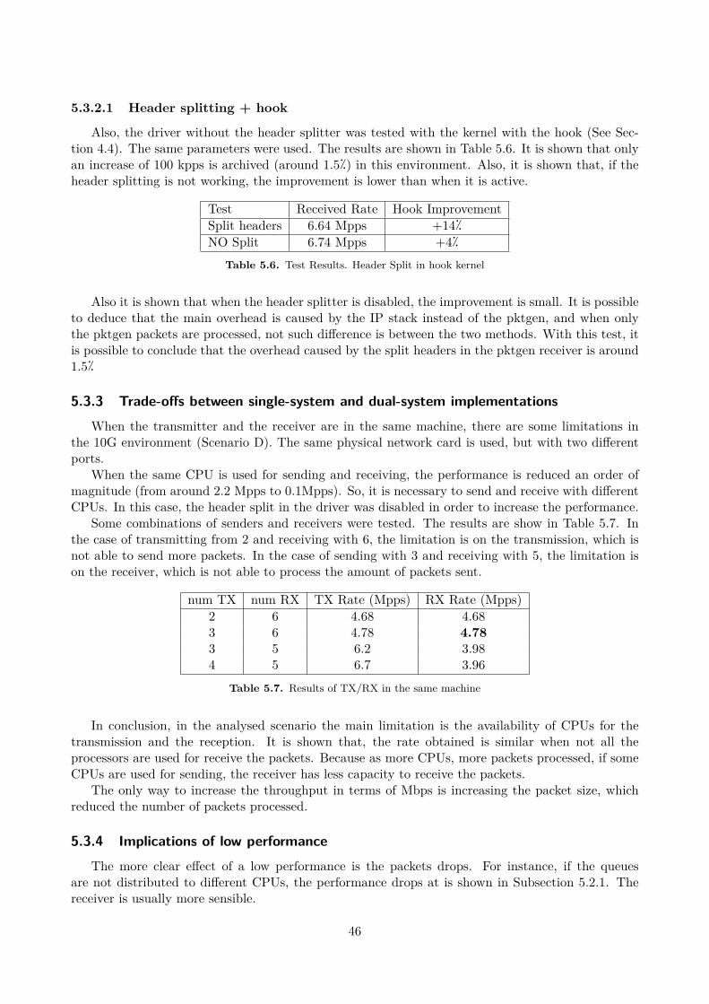
5.3.2.1 Header splitting + hook

Also, the driver without the header splitter was tested with the kernel with the hook (See Sec-tion 4.4). The same parameters were used. The results are shown in Table 5.6. It is shown that onlyan increase of 100 kpps is archived (around 1.5�) in this environment. Also, it is shown that, if theheader splitting is not working, the improvement is lower than when it is active.

Test Received Rate Hook ImprovementSplit headers 6.64 Mpps +14�NO Split 6.74 Mpps +4�

Table 5.6. Test Results. Header Split in hook kernel

Also it is shown that when the header splitter is disabled, the improvement is small. It is possibleto deduce that the main overhead is caused by the IP stack instead of the pktgen, and when onlythe pktgen packets are processed, not such difference is between the two methods. With this test, itis possible to conclude that the overhead caused by the split headers in the pktgen receiver is around1.5�

5.3.3 Trade-offs between single-system and dual-system implementationsWhen the transmitter and the receiver are in the same machine, there are some limitations in

the 10G environment (Scenario D). The same physical network card is used, but with two differentports.

When the same CPU is used for sending and receiving, the performance is reduced an order ofmagnitude (from around 2.2 Mpps to 0.1Mpps). So, it is necessary to send and receive with differentCPUs. In this case, the header split in the driver was disabled in order to increase the performance.

Some combinations of senders and receivers were tested. The results are show in Table 5.7. Inthe case of transmitting from 2 and receiving with 6, the limitation is on the transmission, which isnot able to send more packets. In the case of sending with 3 and receiving with 5, the limitation ison the receiver, which is not able to process the amount of packets sent.

num TX num RX TX Rate (Mpps) RX Rate (Mpps)2 6 4.68 4.683 6 4.78 4.783 5 6.2 3.984 5 6.7 3.96

Table 5.7. Results of TX/RX in the same machine

In conclusion, in the analysed scenario the main limitation is the availability of CPUs for thetransmission and the reception. It is shown that, the rate obtained is similar when not all theprocessors are used for receive the packets. Because as more CPUs, more packets processed, if someCPUs are used for sending, the receiver has less capacity to receive the packets.

The only way to increase the throughput in terms of Mbps is increasing the packet size, whichreduced the number of packets processed.

5.3.4 Implications of low performanceThe more clear effect of a low performance is the packets drops. For instance, if the queues

are not distributed to different CPUs, the performance drops at is shown in Subsection 5.2.1. Thereceiver is usually more sensible.

46

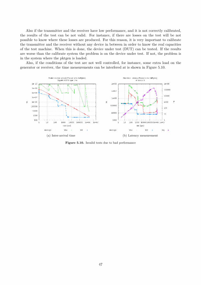
Also if the transmitter and the receiver have low performance, and it is not correctly calibrated,the results of the test can be not valid. For instance, if there are losses on the test will be notpossible to know where these losses are produced. For this reason, it is very important to calibratethe transmitter and the receiver without any device in between in order to know the real capacitiesof the test machine. When this is done, the device under test (DUT) can be tested. If the resultsare worse than the calibrate system the problem is on the device under test. If not, the problem isin the system where the pktgen is loaded.

Also, if the conditions of the test are not well controlled, for instance, some extra load on thegenerator or receiver, the time measurements can be interfered at is shown in Figure 5.10.

(a) Inter-arrival time (b) Latency measurement

Figure 5.10. Invalid tests due to bad performance

47

Chapter 6

Conclusions

In this thesis, some improvements to Pktgen are proposed, designed, implemented and evaluatedin order to convert Pktgen into a network analyser tool. The design was done having in mind theperformance and new features of commodity PCs are used, such as taking advantage of SMP systemsand multiple queues in the network cards. In this work is demonstrated, that multiple queues allowsprocessing the packets in parallel, increasing the scalability of the system. Also, it allows receivingat higher speed if one CPU is not power enough to process all the incoming traffic.

The granularity of Pktgen’s transmission was improved, as well as the way how the user canintroduce the parameters, in order to improve the usability. With the new version, it is possibleto specify a rate in terms of megabits per second or packets per second. Also, the granularityimprovement introduces a more accurate inter-arrival time between packets at low rates, making theflow more constant.

The receiver side statistics, specially the receiver throughput is a powerful tool to evaluate theperformance of the network when it is saturated. The experiments showed that SMP system canreceive and process more packets than a single CPU. On the other hand, the overall performanceis not the sum of the packets processed with single CPU. For each CPU that process packets, lessperformance is achieved per CPU. The overall performance is better, except when Hyperthreadingstarts to work. In this case, the drop does not compensate the additional CPU. But if all CPUswith Hyperthreading are processing packets, the result is higher than without it. Additionally, somefeatures of the cards have a direct impact on the received rate. For instance, the header split (availablein Intel 10G card 82599) reduces the performance of routing capability on the system.

The different type of levels of statistics (Counter, Basic and Time) implemented allow adaptingthe application to different systems with performance limitations. The time statistics (inter-arrivaltimes, jitter and latency) is a powerful tool to understand how the Linux kernel behave, and also itallows monitoring the behaviour of the network. With the inter-arrival statistics has been discoveredthat the transmission pattern depends on the configuration of the system. Moreover, an unexpectedbehaviour is observed in the latency of the network: lower rate has higher latency than higher rates.Usually, the lower latencies should be achieved in lower rates.

Also, it is possible to display the results in two different formats in order to adapt the resultsto the reader. First, the human display includes text description of the parameters. Second, scriptdisplay allows to easily creating scripts to automate tests.

All of the new and modified features are integrated in the current Pktgen module, in order toadd new features to this network tool inside the Linux Kernel. Some of the results open new fieldsof research, and it will allow designing better drivers and operating systems under Linux.

The tools have already tried in different environments and test with satisfactory results at theTelecommunications System Laboratory (TSlab) in the ICT School of KTH. At the time of writing,the result of this thesis is used in four research projects. Moreover, some parts of the code have been

49

sent to the Bifrost [52] and net-next [53] mailing list in order to incorporate the features to the mainLinux Kernel.

6.1 Future workNew applications and new studies can be started with the Pktgen receiver. For instance, the

change of latency with different rates does not follow the traditional curve of network delay. Thedelay in lower rates should be lower than in higher rates, but this is not the case.

Another aspect discovered was that how the delay is used in the Pktgen sender influence theinter-arrival times of the packets. A study of the optimal values for the delay is required to obtain amore constant traffic (CBR).

Moreover, implementing a latency test with some synchronization in order to test the end-to-endlatency can be considered.

50

Bibliography

[1] IXIA - Leader in Converged IP Testing. Available online at http://www.ixiacom.com/. Lastvisited on February 12th, 2010.

[2] IXIA IxNetwork Datasheet. Available online at http://www.ixiacom.com/products/ixnetwork.Last visited on February 15th, 2010.

[3] IXIA IxCharriot. Available online at http://www.ixchariot.com. Last visited on February 15th,2010.

[4] Spirent Smartbits. Available online at http://www.spirent.com/Solutions-Directory/Smartbits.aspx. Last visited on February 15th, 2010.

[5] Sebastian Zander, David Kennedy, and Grenville Armitage. KUTE A High Performance Kernel-based UDP Traffic Engine. Technical Report 050118A, Centre for Advanced Internet Architec-tures, Swinburne University of Technology, Melbourne, Australia, 18 January 2005.

[6] TCPDUMP / Libpcap . Available online at http://www.tcpdump.org/. Last visited on February15th, 2010.

[7] Wireshark Foundation Wireshark. Available online at http://www.wireshark.org/. Last visitedon February 15th, 2010.

[8] Source Fire Snort. Available online at http://www.snort.org/. Last visited on February 15th,2010.

[9] SSLdump. Available online at http://www.rtfm.com/ssldump/. Last visited on February 15th,2010.

[10] Gordon Lyon Nmap. Available online at http://nmap.org/. Last visited on February 15th, 2010.

[11] Justniffer. Available online at http://justniffer.sourceforge.net/. Last visited on February 15th,2010.

[12] Kismet. Available online at http://www.kismetwireless.net/. Last visited on February 15th, 2010.

[13] PerihelMausezahn. Available online at http://www.perihel.at/sec/mz/. Last visited on February15th, 2010.

[14] Ncap. Available online at http://luca.ntop.org/. Last visited on February 15th, 2010.

[15] L. Deri. ncap: Wire-speed packet capture and transmission. IEEE/IFIP Workshop on End-to-End Monitoring Techniques and Services, 2005.

51

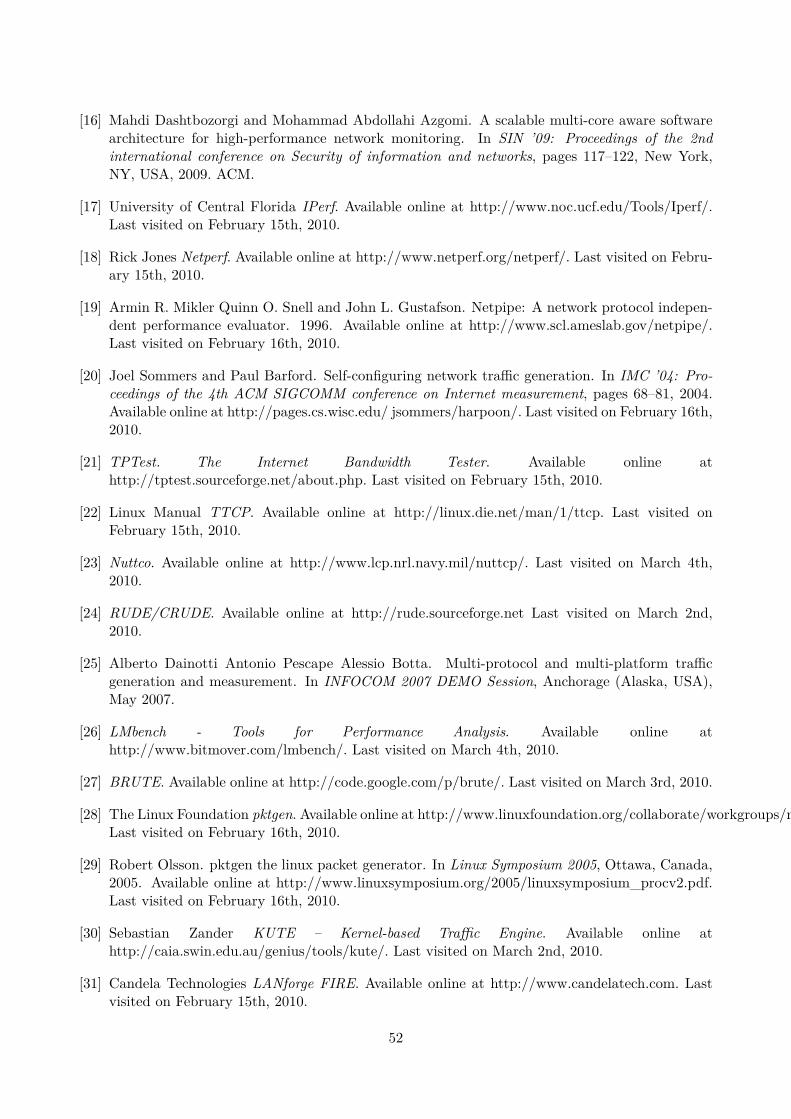
[16] Mahdi Dashtbozorgi and Mohammad Abdollahi Azgomi. A scalable multi-core aware softwarearchitecture for high-performance network monitoring. In SIN ’09: Proceedings of the 2ndinternational conference on Security of information and networks, pages 117–122, New York,NY, USA, 2009. ACM.

[17] University of Central Florida IPerf. Available online at http://www.noc.ucf.edu/Tools/Iperf/.Last visited on February 15th, 2010.

[18] Rick Jones Netperf. Available online at http://www.netperf.org/netperf/. Last visited on Febru-ary 15th, 2010.

[19] Armin R. Mikler Quinn O. Snell and John L. Gustafson. Netpipe: A network protocol indepen-dent performance evaluator. 1996. Available online at http://www.scl.ameslab.gov/netpipe/.Last visited on February 16th, 2010.

[20] Joel Sommers and Paul Barford. Self-configuring network traffic generation. In IMC ’04: Pro-ceedings of the 4th ACM SIGCOMM conference on Internet measurement, pages 68–81, 2004.Available online at http://pages.cs.wisc.edu/ jsommers/harpoon/. Last visited on February 16th,2010.

[21] TPTest. The Internet Bandwidth Tester. Available online athttp://tptest.sourceforge.net/about.php. Last visited on February 15th, 2010.

[22] Linux Manual TTCP. Available online at http://linux.die.net/man/1/ttcp. Last visited onFebruary 15th, 2010.

[23] Nuttco. Available online at http://www.lcp.nrl.navy.mil/nuttcp/. Last visited on March 4th,2010.

[24] RUDE/CRUDE. Available online at http://rude.sourceforge.net Last visited on March 2nd,2010.

[25] Alberto Dainotti Antonio Pescape Alessio Botta. Multi-protocol and multi-platform trafficgeneration and measurement. In INFOCOM 2007 DEMO Session, Anchorage (Alaska, USA),May 2007.

[26] LMbench - Tools for Performance Analysis. Available online athttp://www.bitmover.com/lmbench/. Last visited on March 4th, 2010.

[27] BRUTE. Available online at http://code.google.com/p/brute/. Last visited on March 3rd, 2010.

[28] The Linux Foundation pktgen. Available online at http://www.linuxfoundation.org/collaborate/workgroups/networking/pktgen.Last visited on February 16th, 2010.

[29] Robert Olsson. pktgen the linux packet generator. In Linux Symposium 2005, Ottawa, Canada,2005. Available online at http://www.linuxsymposium.org/2005/linuxsymposium_procv2.pdf.Last visited on February 16th, 2010.

[30] Sebastian Zander KUTE – Kernel-based Traffic Engine. Available online athttp://caia.swin.edu.au/genius/tools/kute/. Last visited on March 2nd, 2010.

[31] Candela Technologies LANforge FIRE. Available online at http://www.candelatech.com. Lastvisited on February 15th, 2010.

52

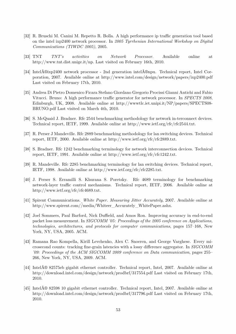
[32] R. Bruschi M. Canini M. Repetto R. Bolla. A high performance ip traffic generation tool basedon the intel ixp2400 network processor. In 2005 Tyrrhenian International Workshop on DigitalCommunications (TIWDC 2005), 2005.

[33] TNT TNT’s activities on Network Processor. Available online athttp://www.tnt.dist.unige.it/np. Last visited on February 16th, 2010.

[34] Intel®ixp2400 network processor - 2nd generation intel®npu. Technical report, Intel Cor-poration, 2007. Available online at http://www.intel.com/design/network/papers/ixp2400.pdfLast visited on February 17th, 2010.

[35] Andrea Di Pietro Domenico Ficara Stefano Giordano Gregorio Procissi Gianni Antichi and FabioVitucci. Bruno: A high performance traffic generator for network processor. In SPECTS 2008,Edinburgh, UK, 2008. Available online at http://wwwtlc.iet.unipi.it/NP/papers/SPECTS08-BRUNO.pdf Last visited on March 4th, 2010.

[36] S. McQuaid J. Bradner. Rfc 2544 benchmarking methodology for network in-terconnect devices.Technical report, IETF, 1999. Available online at http://www.ietf.org/rfc/rfc2544.txt.

[37] R. Perser J Mandeville. Rfc 2889 benchmarking methodology for lan switching devices. Technicalreport, IETF, 2000. Available online at http://www.ietf.org/rfc/rfc2889.txt.

[38] S. Bradner. Rfc 1242 benchmarking terminology for network interconnection devices. Technicalreport, IETF, 1991. Available online at http://www.ietf.org/rfc/rfc1242.txt.

[39] R. Mandeville. Rfc 2285 benchmarking terminology for lan switching devices. Technical report,IETF, 1998. Available online at http://www.ietf.org/rfc/rfc2285.txt.

[40] J. Perser S. Erramilli S. Khurana S. Poretsky. Rfc 4689 terminology for benchmarkingnetwork-layer traffic control mechanisms. Technical report, IETF, 2006. Available online athttp://www.ietf.org/rfc/rfc4689.txt.

[41] Spirent Communications. White Paper. Measuring Jitter Accurately, 2007. Available online athttp://www.spirent.com//̃media/Whiteer_Accurately_WhitePaper.ashx.

[42] Joel Sommers, Paul Barford, Nick Duffield, and Amos Ron. Improving accuracy in end-to-endpacket loss measurement. In SIGCOMM ’05: Proceedings of the 2005 conference on Applications,technologies, architectures, and protocols for computer communications, pages 157–168, NewYork, NY, USA, 2005. ACM.

[43] Ramana Rao Kompella, Kirill Levchenko, Alex C. Snoeren, and George Varghese. Every mi-crosecond counts: tracking fine-grain latencies with a lossy difference aggregator. In SIGCOMM’09: Proceedings of the ACM SIGCOMM 2009 conference on Data communication, pages 255–266, New York, NY, USA, 2009. ACM.

[44] Intel® 82575eb gigabit ethernet controller. Technical report, Intel, 2007. Available online athttp://download.intel.com/design/network/prodbrf/317554.pdf Last visited on February 17th,2010.

[45] Intel® 82598 10 gigabit ethernet controller. Technical report, Intel, 2007. Available online athttp://download.intel.com/design/network/prodbrf/317796.pdf Last visited on February 17th,2010.

53

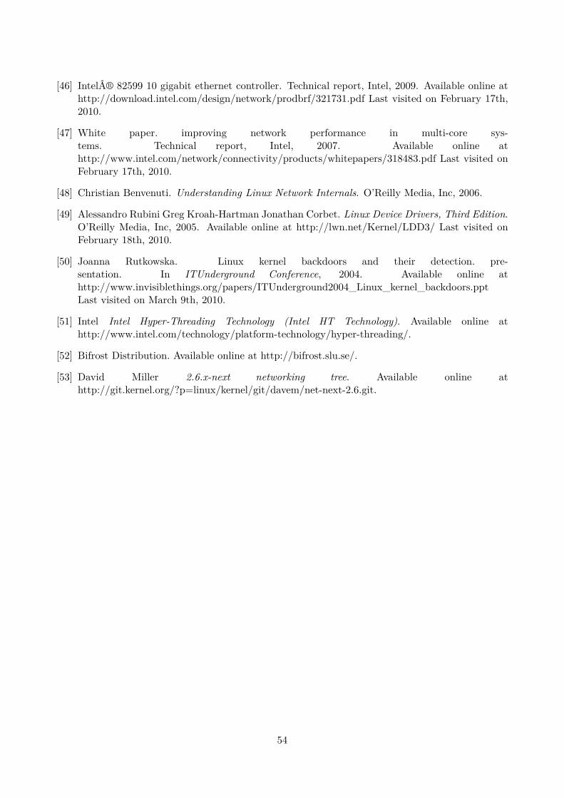
[46] Intel® 82599 10 gigabit ethernet controller. Technical report, Intel, 2009. Available online athttp://download.intel.com/design/network/prodbrf/321731.pdf Last visited on February 17th,2010.

[47] White paper. improving network performance in multi-core sys-tems. Technical report, Intel, 2007. Available online athttp://www.intel.com/network/connectivity/products/whitepapers/318483.pdf Last visited onFebruary 17th, 2010.

[48] Christian Benvenuti. Understanding Linux Network Internals. O’Reilly Media, Inc, 2006.

[49] Alessandro Rubini Greg Kroah-Hartman Jonathan Corbet. Linux Device Drivers, Third Edition.O’Reilly Media, Inc, 2005. Available online at http://lwn.net/Kernel/LDD3/ Last visited onFebruary 18th, 2010.

[50] Joanna Rutkowska. Linux kernel backdoors and their detection. pre-sentation. In ITUnderground Conference, 2004. Available online athttp://www.invisiblethings.org/papers/ITUnderground2004_Linux_kernel_backdoors.pptLast visited on March 9th, 2010.

[51] Intel Intel Hyper-Threading Technology (Intel HT Technology). Available online athttp://www.intel.com/technology/platform-technology/hyper-threading/.

[52] Bifrost Distribution. Available online at http://bifrost.slu.se/.

[53] David Miller 2.6.x-next networking tree. Available online athttp://git.kernel.org/?p=linux/kernel/git/davem/net-next-2.6.git.

54

Appendix A

Source code and scripts

A.1 Kernel patching and compiling

This sections includes a how-to for compiling a Linux kernel from the net-next repository andwith the pktgen patch.

The first necessary thing is donwload the required packatges to build the kernel. In Ubuntu,using pktgen the following command is used:

apt-get install build-essential ncurses-dev git-core kernel-package

Clone the git repository of net-next. It will take some time.

git clone git://git.kernel.org/pub/scm/linux/kernel/git/davem/net-next-2.6.git

Apply the pktgen patch

patch -p1 < [path]/pktgen.patch

Configure the kernel with and compile the kernel.

make menuconfigmakemake modules_installmake install

Usually is a good idea to create a initramfs in order to load the required modules. In order to dothat type:

update-initramfs -c -k [kernel_version]

After the compilation, reboot the system. Finally in order to test the module

modprobe pktgen

A.2 Summary of the new commands added in pktgen

This section includes a summary of the new commands added in pktgen. Some examples ofscripts can be found in Section A.3

55

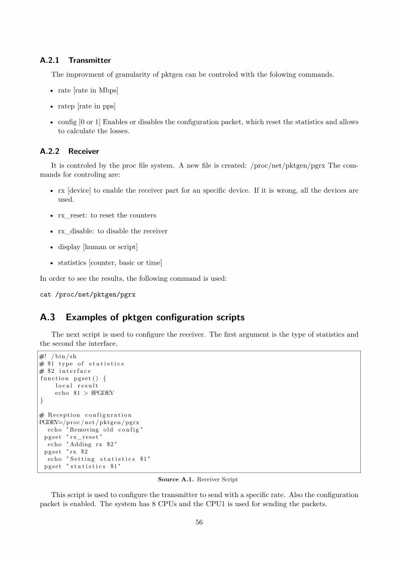
A.2.1 Transmitter

The improvment of granularity of pktgen can be controled with the folowing commands.

• rate [rate in Mbps]

• ratep [rate in pps]

• config [0 or 1] Enables or disables the configuration packet, which reset the statistics and allowsto calculate the losses.

A.2.2 Receiver

It is controled by the proc file system. A new file is created: /proc/net/pktgen/pgrx The com-mands for controling are:

• rx [device] to enable the receiver part for an specific device. If it is wrong, all the devices areused.

• rx_reset: to reset the counters

• rx_disable: to disable the receiver

• display [human or script]

• statistics [counter, basic or time]

In order to see the results, the following command is used:

cat /proc/net/pktgen/pgrx

A.3 Examples of pktgen configuration scriptsThe next script is used to configure the receiver. The first argument is the type of statistics and

the second the interface.#! / bin / sh# $1 type o f s t a t i s t i c s# $2 i n t e r f a c efunc t i on pgset ( ) {

l o c a l r e s u l techo $1 > $PGDEV

}

# Reception c on f i gu r a t i onPGDEV=/proc /net /pktgen/pgrx

echo "Removing o ld c on f i g "pgset " rx_reset "echo "Adding rx $2 "

pgset " rx $2echo " Se t t i ng s t a t i s t i c s $1 "

pgset " s t a t i s t i c s $1 "

Source A.1. Receiver Script

This script is used to configure the transmitter to send with a specific rate. Also the configurationpacket is enabled. The system has 8 CPUs and the CPU1 is used for sending the packets.

56

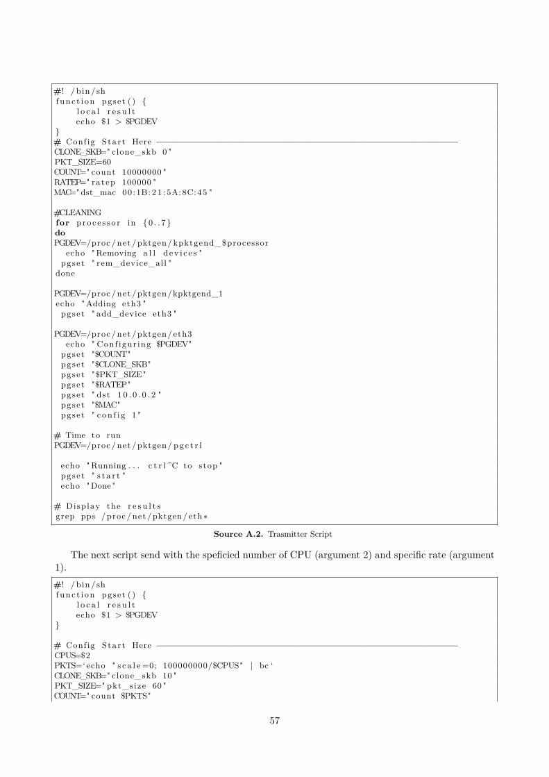
#! / bin / shfunc t i on pgset ( ) {

l o c a l r e s u l techo $1 > $PGDEV

}# Config Sta r t Here −−−−−−−−−−−−−−−−−−−−−−−−−−−−−−−−−−−−−−−−−−−−−−−−−−−−−−−−−−−CLONE_SKB=" clone_skb 0 "PKT_SIZE=60COUNT=" count 10000000 "RATEP=" ratep 100000 "MAC="dst_mac 00 :1B: 2 1 : 5A: 8C:45 "

#CLEANINGfor proc e s s o r in { 0 . . 7 }doPGDEV=/proc /net /pktgen/kpktgend_$processor

echo "Removing a l l d ev i c e s "pgset " rem_device_all "

done

PGDEV=/proc /net /pktgen/kpktgend_1echo "Adding eth3 "pgset " add_device eth3 "

PGDEV=/proc /net /pktgen/ eth3echo " Conf igur ing $PGDEV"

pgset "$COUNT"pgset "$CLONE_SKB"pgset "$PKT_SIZE"pgset "$RATEP"pgset " dst 1 0 . 0 . 0 . 2 "pgset "$MAC"pgset " c on f i g 1 "

# Time to runPGDEV=/proc /net /pktgen/ pg c t r l

echo "Running . . . c t r l ^C to stop "pgset " s t a r t "echo "Done "

# Display the r e s u l t sgrep pps /proc /net /pktgen/ eth ∗

Source A.2. Trasmitter Script

The next script send with the speficied number of CPU (argument 2) and specific rate (argument1).#! / bin / shfunc t i on pgset ( ) {

l o c a l r e s u l techo $1 > $PGDEV

}

# Config Sta r t Here −−−−−−−−−−−−−−−−−−−−−−−−−−−−−−−−−−−−−−−−−−−−−−−−−−−−−−−−−−−CPUS=$2PKTS=‘echo " s c a l e =0; 100000000/$CPUS" | bc ‘CLONE_SKB=" clone_skb 10 "PKT_SIZE=" pkt_size 60 "COUNT=" count $PKTS"

57

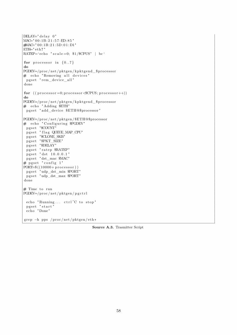
DELAY=" delay 0 "MAC=" 00 :1B: 2 1 : 5 7 :ED:85 "#MAC=" 00 :1B: 2 1 : 5D: 0 1 :D1"ETH=" eth7 "RATEP=‘echo " s c a l e =0; $1/$CPUS" | bc ‘

for proc e s s o r in { 0 . . 7 }doPGDEV=/proc /net /pktgen/kpktgend_$processor# echo "Removing a l l d ev i c e s "pgset " rem_device_all "

done

for ( ( p ro c e s s o r =0; proces sor<$CPUS; p ro c e s s o r++))doPGDEV=/proc /net /pktgen/kpktgend_$processor# echo "Adding $ETH"pgset " add_device $ETH@$processor "

PGDEV=/proc /net /pktgen/$ETH@$processor# echo " Conf igur ing $PGDEV"pgset "$COUNT"pgset " f l a g QUEUE_MAP_CPU"pgset "$CLONE_SKB"pgset "$PKT_SIZE"pgset "$DELAY"pgset " ratep $RATEP"pgset " dst 1 0 . 0 . 0 . 1 "pgset " dst_mac $MAC"

# pgset " c on f i g 1 "PORT=$((10000+ proc e s s o r ) )pgset " udp_dst_min $PORT"pgset "udp_dst_max $PORT"

done

# Time to runPGDEV=/proc /net /pktgen/ pg c t r l

echo "Running . . . c t r l ^C to stop "pgset " s t a r t "echo "Done "

grep −h pps /proc /net /pktgen/ eth ∗

Source A.3. Trasmitter Script

58

www.kth.se

TRITA-ICT-EX-2010:125