Embed Size (px)
Citation preview

Remote Sens. 2015, 7, 9292-9310; doi:10.3390/rs70709292
remote sensing ISSN 2072-4292
www.mdpi.com/journal/remotesensing
Article
Joint Quality Measure for Evaluation of
Pansharpening Accuracy
Gintautas Palubinskas
Remote Sensing Technology Institute, German Aerospace Center (DLR), Oberpfaffenhofen,
82234 Wessling, Germany; E-Mail: [email protected];
Tel.: +49-8153-28-1490; Fax: +49-8153-28-1444.
Academic Editors: Giles Foody, Josef Kellndorfer and Prasad S. Thenkabail
Received: 17 April 2015 / Accepted: 9 July 2015 / Published: 21 July 2015
Abstract: A new Joint Quality Measure (JQM), which is a sole measure, is proposed for
quality ranking of pansharpening methods. It is based on a newly proposed Composite
similarity measure, which consists of Means, Standard deviations and Correlation coefficient
(CMSC), and is translation invariant with respect to means and standard deviations. The JQM
itself consists of a weighted sum of two terms. The first term is measured between a low pass
filtered pansharpened image and original multispectral image at a reduced/low resolution
scale. The second term is measured between the intensity calculated from spectrally weighted
pansharpened multispectral image and original panchromatic image in a high resolution scale.
Experimental results show advantages of a new measure, JQM, for quality assessment of
pansharpening methods on the one hand, and drawbacks or unexpected properties of the
already known measure, Quality with No Reference (QNR), on the other hand.
Keywords: image fusion; multi-resolution; low pass filtering; quality assessment;
similarity measure
1. Introduction
Pansharpening aims to include spatial/detail information from a high resolution image into a low
resolution image while preserving spectral properties of a low resolution image. For example, a high
resolution image is a panchromatic/multispectral image, and a low resolution image is a
multi-spectral/hyper-spectral image. A large number of algorithms and methods to solve this problem
were introduced during the last two decades, which can be divided into two main groups. The first group
OPEN ACCESS
Remote Sens. 2015, 7 9293
of methods is based on a linear spectral transformation, e.g., Intensity-Hue-Saturation (IHS), Principal
Component Analysis, and Gram-Schmidt orthogonalization (GS), followed by a Component
Substitution (CS). Methods of the second group use spatial frequency decomposition usually performed
by means of high pass filtering, e.g., boxcar filter in signal domain, filtering in Fourier domain or
Multi-Resolution Analysis (MRA) using wavelet transform. Here I have to mention that there are some
attempts to combine both types of methods. Moreover, there exist a group of methods which state the
pansharpening task as an ill-posed recovery problem solved by regularization using Bayesian estimation
and recently proposed sparse representation approaches. For recent surveys of various image fusion
methods see publications [1–4].
In parallel to the development of pansharpening methods, many attempts were undertaken to assess
quantitatively their quality usually using measures originating from signal/image processing such as Mean
Squared Error (MSE), Peak Signal-to-Noise Ratio (PSNR), relative dimensionless global error in synthesis
(ERGAS), Pearson’s Correlation Coefficient (CC), Spectral Angle Mapper (SAM), Universal Image Quality
Indices (UIQI/SSIM) and their multispectral extensions (Q4/Q2n). For recent overviews of quality measures,
see references [5,6]. These simple/separate measures defined in scalar/vector form can be used only as Full
Reference (FR) measure, that is, when the reference image is available. This situation is valid for quite few
applications mostly simulations. Due to the missing reference in pansharpening quality assessment task
different solutions or so-called protocols were proposed: Wald’s protocol [7], Zhou’s protocol [8], Quality
with No Reference (QNR) [9] and Khan’s protocol [10], which usually include the calculation of several
quality measures. Of course, a sole or joint quality measure, as already proposed in [9,11,12], enables much
easier and practical/comfortable ranking of various fusion methods.
Usually pansharpening in image processing is used to increase visual quality of an image. In remote
sensing, this task is fully different because it aims at enhancing image quality for further processing such
as clustering, classification, matching and change detection thus requiring only relative comparison of
data (so-called image value/intensity translation invariant applications). For example, the quality
measure UIQI/SSIM [13] was designed for perceptual tasks or scale invariant applications, but recently
it is spreading widely in other applications. Thus, its usage in pansharpening quality assessment in
remote sensing imagery, e.g., QNR [9] and joint quality measures [11,12], can lead to wrong results.
Because MSE and UIQI/SSIM based measures are not very suitable for translation invariant with respect
to sample means and standard deviations applications [14], I propose to exchange/replace the
above-mentioned UIQI/SSIM measures with a new measure—composite measure—based on means,
standard deviations and correlation coefficient (CMSC) [14], which is translation invariant with respect
to means and standard deviations, thus enhancing measures proposed in [12].
In this paper, I perform a comparison of six pansharpening methods originating from the main earlier
mentioned groups of methods and several parameter settings using a new joint quality measure (JQM)
and already known measure of QNR for IKONOS and WorldView-2 satellite data.
2. Quality Assessment Measures
In this section, I will review/summarize several possible ways and strategies to assess the quality of
pansharpening methods and additionally introduce a new joint quality measure.

Remote Sens. 2015, 7 9294
2.1. Full Reference Measures
Quality or similarity measures can be divided into two main groups: Full reference measures when the
reference image is existent and no reference measures. The latter case is more frequent because in most
applications the reference is missing. Examples of FR measures (scalar or vector based) used to assess
pansharpening quality are SAM, MSE and measures based on it, e.g., PSNR, Relative Average Spectral
Error (RASE) and ERGAS, CC, universal image quality indices (UIQI/SSIM) and multispectral extensions
of UIQI (Q4/Q2n) just to mention few or most popular of them. Deep understanding of the properties of
distance or similarity measures is important in order to use them correctly in a particular application.
Perhaps the two most important properties of the distance measures are: Translation invariance
),(),( 2121 ppdcpcpd (1)
and scale invariance
),(),( 2121 ppdpcpcd (2)
defined for all variables/parameters pi and some fixed constant c. From Equation (1) follows directly
constant),( cppd (3)
for all p and some fixed c, which means that translation invariance implies an independence of the
measure on the absolute parameter values or equivalently dependence only on the relative relation, e.g.,
difference of the parameters. For example, correlation coefficient is both translation and scale invariant
with respect to original data values x, y. Thus, the selection of a particular measure is application
dependent. For example for image matching, clustering or classification applications translation
invariant measures such as MSE can be more suitable. For visual perception applications scale invariant
measures such as UIQI/SSIM are preferable.
It was shown in [14] that MSE based measures are not translation invariant with respect to sample
standard deviation. The recently widely spreading UIQI/SSIM measure is not translation invariant with
respect to both sample moments—means and standard deviations. This can lead to false quality
assessment results in applications such as classification, clustering, matching and change detection,
which usually require translation invariance property Equation (1) or equivalently only relative
comparison of parameters independent of their absolute values Equation (3). Pansharpening products in
remote sensing are mostly used for further processing in the above-mentioned applications. Thus, a new
quality measure CMSC, which is translation invariant with respect to means and standard
deviations [14], can be more suitable/justified
,
2/
)(,,)1(1),(
2
2
22
2
121R
dR
dddyxCMSCyxyx
(4)
where 𝜇𝑥,𝑦 and 𝜎𝑥,𝑦are means and standard deviations for two signal/image patches x, y; ρ is Pearson’s
correlation coefficient and R = 28 − 1 = 255 for 8bit data.
I have to note that there exist some attempts to measure image quality without reference mostly based
on gradients in an image [15]. However, they are not sensitive/subtle enough to measure fine differences
that usually occur during pansharpening processes. Thus, the following practical approaches have been
established over the past two decades and are presented in the following Section 2.3.

Remote Sens. 2015, 7 9295
2.2. Application Based Quality Assessment
As the reference image is not available in pansharpening applications an ideal or objective way to assess
quality of pansharpening products would be to evaluate their impact in a particular application by using
reference/ground truth data of a given application. This way is very time- and resource-consuming and is
thus is not practical in the selection of a suitable method from the hundreds of methods available [3].
2.3. Quality Assessment Based on Comparison with Input Data
A practical way of quality assessment is based on the comparison of a fusion result with the two
inputs of pansharpening: Low resolution multispectral image msk (k is the index of the spectral band)
and high resolution panchromatic image pan.
2.3.1. Quality Assessment Based on an Original Multispectral Image at Low Resolution Scale
For this type of comparison, the following two approaches have been established during the two
past decades.
In the first approach, the multispectral fusion result msfk in a high resolution scale is compared with
the original multispectral image msk, which is available at a low resolution scale. This is so that the high
resolution pansharpened image should be low pass filtered and decimated to the resolution of original
multispectral image. This way of pansharpening quality assessment is known as a consistency or Wald’s
protocol first property [7,16]. Any FR measure mentioned in Section 2.1 can be used for this purpose.
Usually, the cutoff frequency of a low pass filter is equal to the ratio of high resolution to low resolution.
In Khan’s protocol [10], the cutoff frequencies of low pass filters are derived from instrument based
spectral Modulation Transfer Functions (MTFs).
The recently proposed spectral distortion measure Dλ, which is a one part of QNR protocol [9], avoids
preprocessing of the fused result by comparing inter-band UIQI values separately calculated at
different resolutions
N
kl
klkl msfmsfUIQImsmsUIQINN
D1,
),(),()1(
1 (5)
where N is the number of bands. Unfortunately, evidence or proof that such inter-band relations hold
between resolution scales is not provided or missing. Moreover, such inter-band comparison of different
spectral bands is possible mathematically, but is incorrect physically because different parts of spectrum
or more generally content/information are compared which may be incommensurable.
I propose to enhance the Quality measure at Low Resolution (QLR) proposed in [12] by replacing
the SSIM with a newly introduced CMSC Equation (4) [14] and additionally including sensor spectral
response function gains to account for different spectral overlap of multispectral and panchromatic
bands. Thus, QLR is defined in a reduced resolution space and compares only multispectral images
which are spectrally overlapping with the panchromatic band
N
klpfkkk msfmsCMSCwQLR
1, ),( (6)

Remote Sens. 2015, 7 9296
where wk—spectral response weight for band k, which is calculated from spectral response functions of
data provider [17], 𝑚𝑠𝑓𝑘,𝑙𝑝𝑓 = (𝑚𝑠𝑓𝑘 ∗ 𝑙𝑝𝑓𝑘) ↓, lpfk—a Gaussian low pass filter which can be band
dependent, *—convolution operator, ↓ means decimating of high resolution data to a low resolution
scale. Thus, two new enhancements of [12] are introduced: A new FR measure CMSC and the spectral
weights wk. Moreover, this measure is spectrally consistent or physically correct in that sense that it
compares the commensurable information or the same parts (bands) of electromagnetic spectrum.
In the second approach proposed by Wald [7,16] also known as a synthesis property (Wald’s protocol
second and third property) a fused multi-band result is compared with a reference in high resolution
separately for each band and using inter-band relations. Due to the missing reference at high resolution
the following preprocessing of data to reduced resolution scale is performed. Input data msk and pan are
low pass filtered and decimated by a factor equal to the resolution scale ratio of pan to msk images: msk,lpf
and panlpf. Then pansharpening of msk,lpf using panlpf is performed. The result of fusion msfk,lpf is
compared with original multispectral msk images (true reference in this case) using any FR measure
mentioned in Section 2.1. Unfortunately, evidence or proof that quality assessment results/conclusions
obtained in a reduced resolution scale hold for a high resolution scale is not given or missing.
Measures discussed in this Sub-section estimate the spectral quality of a fusion result (so-called
spectral consistency) and are necessary for pansharpening quality assessment. However, they are not
sufficient because, e.g., simple nearest neighbor interpolation will outperform all pansharpening
methods. Thus, an additional quality assessment in a high resolution scale is necessary to evaluate fusion
results correctly.
2.3.2. Quality Assessment based on Panchromatic Image in High Resolution Scale
As already mentioned above, due to the missing reference in the high resolution, only comparison of
the fusion result msfk with the high resolution panchromatic image pan can be performed. Usually, this
comparison is based on the edge information. In Zhou’s protocol, for example, details are extracted using
Laplacian filter and then correlation coefficient is used as a quality measure [8]. The recently proposed
spatial distortion measure Ds (one part of QNR protocol [9]) compares inter-band UIQI values pair-wise:
Between the fused msfk and the panchromatic image pan, and the low resolution multispectral image msk
and the low pass filtered panchromatic panlpf image
N
k
klpfks panfmsUIQIpanmsUIQIN
D1
),(),(1
(7)
where, panlpf = pan*lpf. In Khan’s protocol [10] MTF based filters are used to extract high frequency
information and the UIQI measure is used for comparison. In [18] MTFs are estimated automatically
from the edge information in an image which makes this approach even more practical. Unfortunately,
evidence or proof that such comparison of different spectral bands (narrow multispectral band and broad
panchromatic band) is legitimate is missing. Moreover, it is incorrect physically or spectrally
inconsistent because different spectrum parts or more generally content/information is compared, which
may be incommensurable.
Thus, I propose a Quality measure at High Resolution (QHR) which is defined at a high resolution
scale [12]. This measure compares the intensity calculated from a weighted sum of multispectral bands
(simulated panchromatic image) Imsf with the original pan image

Remote Sens. 2015, 7 9297
),( msfIpanCMSCQHR (8)
where
N
k
kkmsf msfwI1
. (9)
For this measure, QHR, the two new enhancements of [12] are introduced: the new FR measure
CMSC and spectral weights wk calculated from spectral response functions of data provider [17]. This
measure is spectrally (physically) consistent because it compares the same portions (bands) of the
electromagnetic spectrum. I have to note that this measure includes a check of both spectral and spatial
properties of a fusion result. Thus, the following application scenario is possible. For example, if QLR
is quite high (good spectral quality) then QHR can be used to compare the spatial quality of a fusion
result. Moreover, this measure can act well as a sole measure if no other measures are available because
it evaluates both properties of image quality.
2.3.3. Joint Quality Measures based on Both Inputs
Previously, discussed assessment methods (Sections 2.3.1 and 2.3.2) lead to a set of measures derived
in low and high resolution scales sometimes called protocols, e.g., Zhou’s protocol [8] and Khan’s
protocol [10]. It is observed that it is quite difficult to rank methods using several measures thus sole or
joint measures (produced by averages or products of separate measures) were proposed recently such as
QNR [9], product of two measures [11] and JQM [12]. For example, QNR is defined as a product of two
separate measures presented in Equations (5) and (7)
)1()1( sDDQNR (10)
Whereas JQM is defined as a weighted sum of separate measures presented in Equations (6) and (8)
1, 2121 vvQHRvQLRvJQM (11)
Equal weights vi = 0.5 are used in this paper. These two joint measures and their corresponding separate
measures are employed in this paper to assess quality of pansharpening methods. The ranges of all
similarity measures and their compound parts are limited to interval (0, 1) by clipping negative correlation
coefficient values to 0 in UIQI and CMSC measures, where one is achieved for identical values.
3. Experimental Results
I will illustrate my ideas concerning pansharpening quality assessment for two optical remote sensing
satellites IKONOS and WorldView-2 (WV-2) over Munich, Germany. For scene details see Table 1.
In this section, I will compare six different pansharpening methods (see Section 3.1) and several parameter
settings using the proposed JQM and already known QNR joint quality measures, and additionally
well-established spectral measures SAM and ERGAS. First, the interpolation influence is only investigated
by comparing the four most popular interpolation methods (Section 3.2). Second, the interpolation method
influence on one of the pansharpening methods is analyzed in Section 3.3. Finally, the comparison of various
pansharpening methods and their parameter settings is presented in Section 3.4.

Remote Sens. 2015, 7 9298
Table 1. Scene parameters for Ikonos and WorldView-2 data over the city of Munich, Germany.
Sensor Parameter IKONOS WorldView-2
Image date 15 July 2005 12 July 2010
Image time (local) 10:28:06 10:30:17
Mode PAN+MS PAN+MS
Look angle 5° Right 5.2° Left
Product L2A L2A
Resolution PAN (m) 1.0 0.5
Resolution MS (m) 4.0 2.0
3.1. Pansharpening Methods
Methods investigated in this paper can be described by the following general expression (see e.g., [1,19,20])
)( lpfkkk panpangmsimsf (12)
where msfk—fused/pansharpened high resolution multispectral image, k—spectral band number,
msik—low resolution multispectral image interpolated to a high resolution space, gk—weight (gain) for
detail injection, pan—high resolution panchromatic image and panlpf—low pass filtered pan image.
Usually histogram matching of msfk and msk is performed after application of Equation (12). Then,
individual methods can be seen as special cases of Equation (12) as shown below.
General Fusion Filtering (GFF) [21] is defined as
,)1()()(1 LPFpanFFTmsFFTWZPFFTmsf kk (13)
where gk = 1, msk—low resolution multispectral image, ZP—zero padding interpolation, W—Hamming
window for ringing artifacts suppression and LPF—low pass filter in Fourier domain.
High Pass Filtering Method HPFM (variant of GFF) [22] is given by
lpfkk panpanmsimsf (14)
with gk = 1, panlpf = pan*lpf, lpf = FFT−1(LPF), where lpf is a Gaussian low pass filter in signal domain.
Here, I have to note that the cutoff frequency of a low pass filter can be selected individually for each
spectral band as, e.g., already proposed for MRA based methods using modulation transfer function
(MTF) information [23].
Ehlers fusion [24] is defined as
21 lpfpanpanlpfIImsimsf msimsikk (15)
where gk = 1, intensity is defined as
kkmsi msiwI (16)
wk are spectral weights calculated from spectral response functions of data provider [17]. Two different
low pass filters are used for filtering of pan and intensity images, respectively. Usually original software
of the method is not available, thus the author’s software implementation is used.
Á trous wavelet transform ATWT [25] is given by Equation (12) with gk = 1 and panlpf—à trous
wavelet decomposed low resolution version of pan. M. Canty’s software implementation [26] is used.

Remote Sens. 2015, 7 9299
Component substitution using IHS transformation (CS IHS) can be written as follows
panImsimsf msikk (17)
with gk = 1, panlpf = Imsi, and Imsi is defined by Equation (16). The author’s software implementation is
used. Here, I have to note that QHR = 1 for this method what contradicts not to the already known high
spatial quality of this method. Thus, usage of an additional measure, e.g., QLR or JQM will allow
correctly to discriminate it from other pansharpening methods.
Component substitution using GS transformation (CS GS) is Equation (12) with panlpf = Imsi.
IDL ENVI 5.0 software implementation is used.
3.2. Interpolation Influence Only
Values of both joint quality measures JQM and QNR and their corresponding separate measures
(QLR, QHR and DL, DS) are presented in Figures 1–4 for differently interpolated multispectral data
(high resolution scale) of IKONOS (Figures 1 and 2) and WV-2 sensors (Figures 3 and 4). The following
interpolation methods are investigated: nearest neighbor (NN), zero padding using Fourier transform
(ZP), bilinear interpolation (BIL) and cubic convolution (CUB) (IDL ENVI 5.0 software is used except
ZP, which is the author’s software implementation).
We see that all interpolation methods exhibit quite similar QLR values for both sensors (Figures 1b and 3b).
For example, this is well supported by visual analysis of interpolation results presented in Figure 5. All methods
exhibit similar colors or multispectral information. Similarly, all methods have quite similar QHR values except
NN. NN has very poor spatial quality. This can be observed in Figure 5a. These results lead to low (poor) values
of JQM for NN for both sensors (Figures 1a and 3a). Moderately oscillating values of separate measures QLR
and QHR for the other three methods result in slightly higher values of CUB for IKONOS (Figure 1a) and ZP
for WV-2 (Figure 3a).
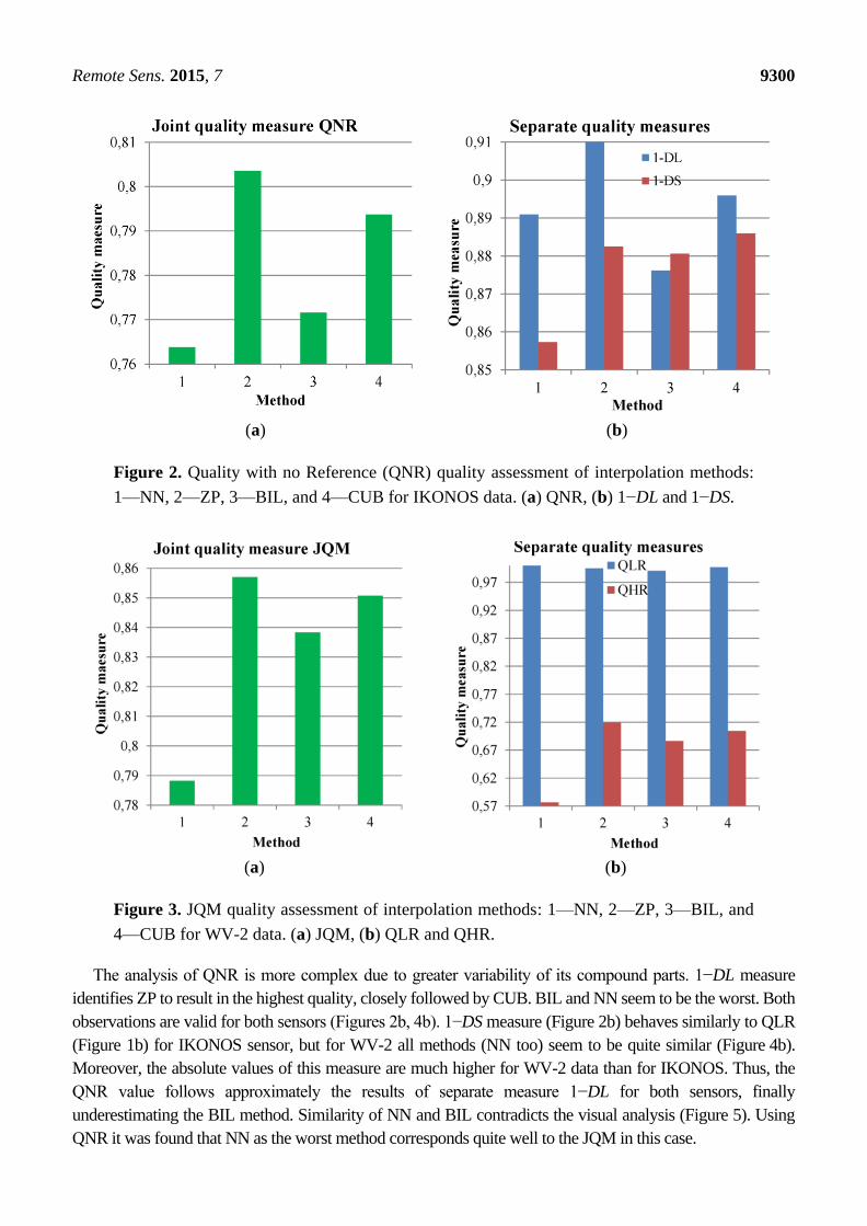
(a) (b)
Figure 1. Joint Quality Measure (JQM) quality assessment of interpolation methods:
1—nearest neighbor (NN), 2—zero padding (ZP), 3—bilinear interpolation (BIL), and
4—cubic convolution (CUB) for IKONOS data. (a) JQM, (b) QLR and QHR.
Remote Sens. 2015, 7 9300
(a) (b)
Figure 2. Quality with no Reference (QNR) quality assessment of interpolation methods:
1—NN, 2—ZP, 3—BIL, and 4—CUB for IKONOS data. (a) QNR, (b) 1−DL and 1−DS.
(a) (b)
Figure 3. JQM quality assessment of interpolation methods: 1—NN, 2—ZP, 3—BIL, and
4—CUB for WV-2 data. (a) JQM, (b) QLR and QHR.
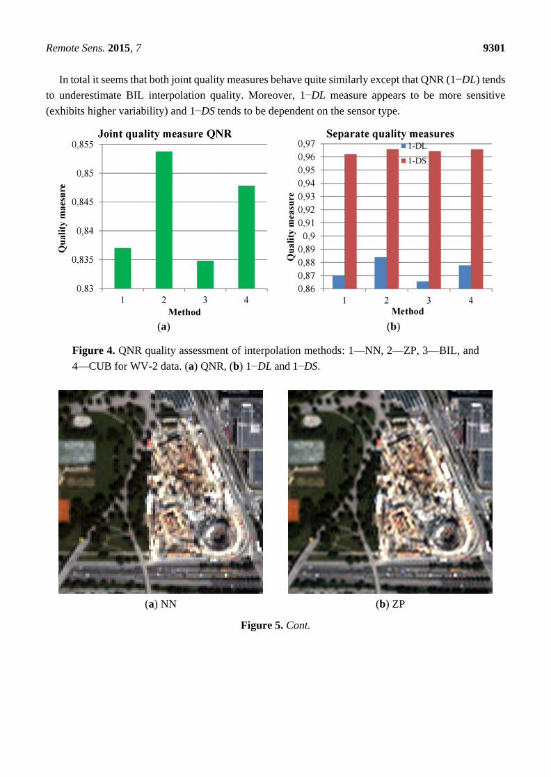
The analysis of QNR is more complex due to greater variability of its compound parts. 1−DL measure
identifies ZP to result in the highest quality, closely followed by CUB. BIL and NN seem to be the worst. Both
observations are valid for both sensors (Figures 2b, 4b). 1−DS measure (Figure 2b) behaves similarly to QLR
(Figure 1b) for IKONOS sensor, but for WV-2 all methods (NN too) seem to be quite similar (Figure 4b).
Moreover, the absolute values of this measure are much higher for WV-2 data than for IKONOS. Thus, the
QNR value follows approximately the results of separate measure 1−DL for both sensors, finally
underestimating the BIL method. Similarity of NN and BIL contradicts the visual analysis (Figure 5). Using
QNR it was found that NN as the worst method corresponds quite well to the JQM in this case.
Remote Sens. 2015, 7 9301
In total it seems that both joint quality measures behave quite similarly except that QNR (1−DL) tends
to underestimate BIL interpolation quality. Moreover, 1−DL measure appears to be more sensitive
(exhibits higher variability) and 1−DS tends to be dependent on the sensor type.
(a) (b)
Figure 4. QNR quality assessment of interpolation methods: 1—NN, 2—ZP, 3—BIL, and
4—CUB for WV-2 data. (a) QNR, (b) 1−DL and 1−DS.
(a) NN (b) ZP
Figure 5. Cont.

Remote Sens. 2015, 7 9302
(c) BIL (d) CUB
Figure 5. Different interpolation methods: NN (a), ZP (b), BIL (c) and CUB (d) for the
IKONOS data.
To enhance previously presented experiment, the separate quality measures 1−QLR and DL are
additionally compared with two well established quality measures SAM (given in degrees) and ERGAS
in Figure 6 for IKONOS data. Here, the low measure values stand for similar images. One can see that
all measures, except DL, correlate quite well with each other (Figure 6a–c). Thus, a new measure QLR
is legitimated for a practical usage in pansharpening quality assessment. The DL measure behaves
unexpectedly for NN and ZP by underestimating the quality of NN and overestimating ZP. The reason
for that can be the violation of the assumption about the preservation of between-band relations in
different resolution scales. Similar results are observed for other experiments of this paper and sensor
WV-2 data.
(a) (b)
Figure 6. Cont.

Remote Sens. 2015, 7 9303
(c) (d)
Figure 6. Quality assessment of interpolation methods: 1—NN, 2—ZP, 3—BIL, and
4—CUB for IKONOS data using different separate quality measures. (a) 1−QLR, (b) SAM,
(c) ERGAS, (d) DL.
3.3. Interpolation Influence on the HPFM Pansharpening Method
The JQM quality of a selected pansharpening method using different interpolation methods is shown in
Figures 7 and 8. In this case, the HPFM with a cutoff frequency 0.15 for IKONOS and WV-2 data is used.
(a) (b)
Figure 7. JQM quality assessment of High Pass Filtering Method (HPFM) for different
interpolation methods: 1—NN, 2—ZP, 3—BIL, and 4—CUB for IKONOS data. (a) JQM,
(b) QLR and QHR.
Remote Sens. 2015, 7 9304
(a) (b)
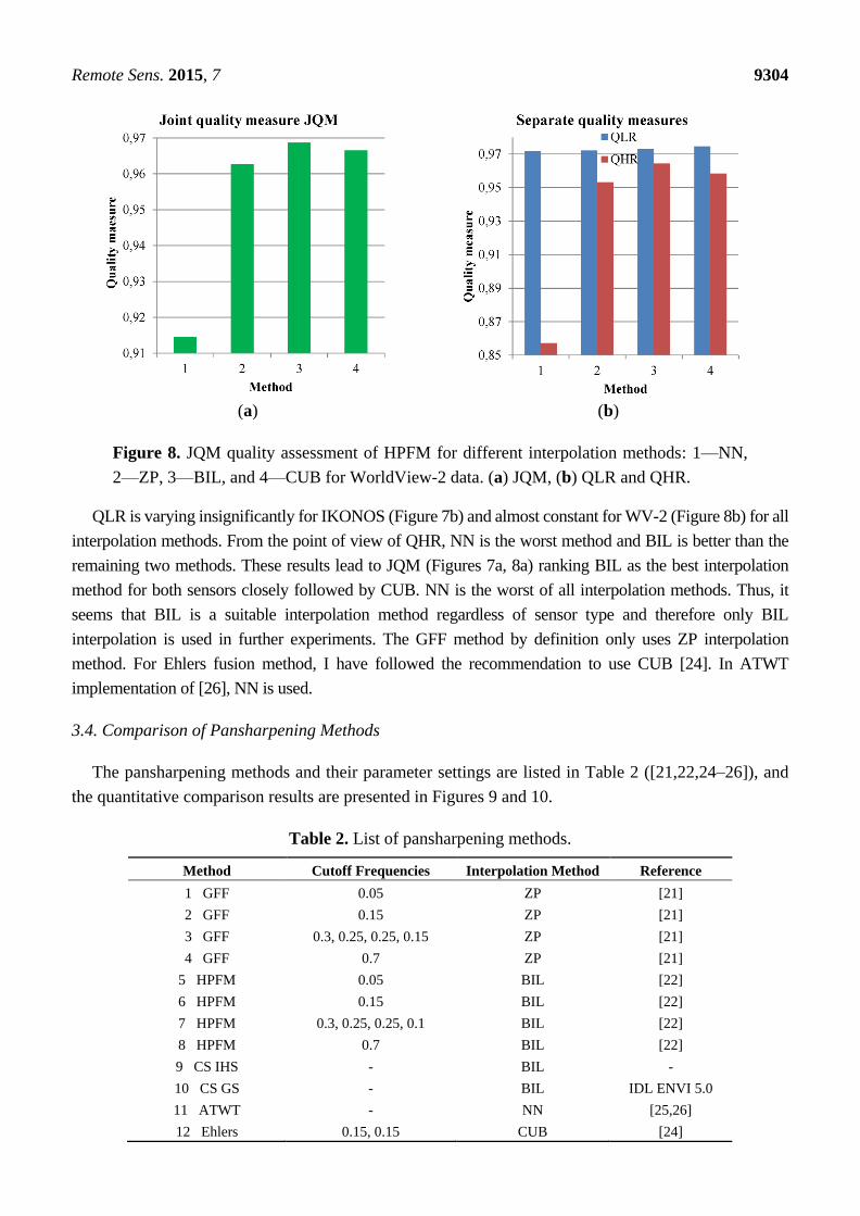
Figure 8. JQM quality assessment of HPFM for different interpolation methods: 1—NN,
2—ZP, 3—BIL, and 4—CUB for WorldView-2 data. (a) JQM, (b) QLR and QHR.
QLR is varying insignificantly for IKONOS (Figure 7b) and almost constant for WV-2 (Figure 8b) for all
interpolation methods. From the point of view of QHR, NN is the worst method and BIL is better than the
remaining two methods. These results lead to JQM (Figures 7a, 8a) ranking BIL as the best interpolation
method for both sensors closely followed by CUB. NN is the worst of all interpolation methods. Thus, it
seems that BIL is a suitable interpolation method regardless of sensor type and therefore only BIL
interpolation is used in further experiments. The GFF method by definition only uses ZP interpolation
method. For Ehlers fusion method, I have followed the recommendation to use CUB [24]. In ATWT
implementation of [26], NN is used.
3.4. Comparison of Pansharpening Methods
The pansharpening methods and their parameter settings are listed in Table 2 ([21,22,24–26]), and
the quantitative comparison results are presented in Figures 9 and 10.
Table 2. List of pansharpening methods.
Method Cutoff Frequencies Interpolation Method Reference
1 GFF 0.05 ZP [21]
2 GFF 0.15 ZP [21]
3 GFF 0.3, 0.25, 0.25, 0.15 ZP [21]
4 GFF 0.7 ZP [21]
5 HPFM 0.05 BIL [22]
6 HPFM 0.15 BIL [22]
7 HPFM 0.3, 0.25, 0.25, 0.1 BIL [22]
8 HPFM 0.7 BIL [22]
9 CS IHS - BIL -
10 CS GS - BIL IDL ENVI 5.0
11 ATWT - NN [25,26]
12 Ehlers 0.15, 0.15 CUB [24]

Remote Sens. 2015, 7 9305
The QLR measure behaves as expected for GFF (methods 1–4) and HPFM (methods 5–8) in
dependence of the cutoff frequencies (Figure 9b). That is, QLR increases with the increase of cutoff
frequency (spectral quality). QHR identifies methods 2 and 6 as the best, which correspond quite well with
visual analysis in Figure 11d. For example, the image in Figure 11d exhibits much better spatial quality
than the image in Figure 11f. Further, JQM selects methods 3 and 7 with band dependent cutoff frequencies
(Figure 9a), which is well supported by visual interpretation in Figure 11. For example, the image in
Figure 11e exhibits better spectral quality (e.g., compare with BIL in Figure 11a) than the image in
Figure 11d simultaneously preserving good spatial quality. Moreover, it seems that HPFM, the faster
variant of GFF, is better than GFF, maybe, due to the different interpolation method used. Thus, both
measures QHR and JQM are able to correctly select optimal cutoff frequencies for both methods.
(a) (b)
Figure 9. JQM and separate measures for 6 methods and their different parameter settings
for IKONOS data. (a) JQM, (b) QLR and QHR.
(a) (b)
Figure 10. QNR and separate measures for 6 methods and their different parameter settings
for IKONOS data. (a) QNR, (b) 1−DL and 1−DS.
Spectral measure 1−DL follows approximately the behavior of QLR for methods 1–8 (Figure 10b).
Spatial measure 1−DS again follows the trend of 1−DL, which contradicts visual analysis in Figure 11.
An example is Figure 11f, the image with the estimated highest spatial quality exhibits in reality low
quality when compared to Figure 11d,e. Such behavior of these two measures leads to the same trend of

Remote Sens. 2015, 7 9306
the joint quality measure QNR in Figure 10a. Thus, QNR is not able to select optimal cutoff frequencies
for GFF and HPFM methods.
QLR of other methods: CS IHS (method 9 in Table 2), CS GS (method 10), ATWT (method 11) and
Ehlers (method 12) is lower than those of most filtering methods, whereas for QHR the opposite
observation is valid. Finally, JQM of these methods 9–12 is lower than those of the best filtering methods
2–3, 6–7. For example, low JQM of method 10 is well illustrated visually in Figure 12. The colors of the
image in Figure 12b are significantly different from those of BIL interpolation in Figure 11a or the best
pansharpening method 7 in Figure 11e. QNR ranks methods 9–12 close to methods 1, 5 with high spatial
quality. Only Ehlers (method 12) receives a high overall score.
(a) msik BIL (b) pan
(c) HPFM 0.05 (d) HPFM 0.15
Figure 11. Cont.

Remote Sens. 2015, 7 9307
(e) HPFM 0.3, 0.25, 0.25, 0.1 (f) HPFM 0.7
Figure 11. Bilinear interpolated bands: 3, 2, 1 (a), panchromatic band (b) and HPFM fusion
with variable image quality controlled by parameters: 0.05 (c), 0.15 (d), band dependent
parameters: 0.3, 0.25, 0.25, 0.1 (e) and 0.7 (f) for IKONOS data.
(a) CS IHS (b) CS GS
Figure 12. Cont.
Remote Sens. 2015, 7 9308
(c) ATWT (d) Ehlers
Figure 12. Different fusion methods: CS IHS (a), CS GS (b), ATWT (c) and Ehlers (d) for
IKONOS data.
In conclusion, I mention one more observation or drawback of QNR limiting its practical usage. JQM
values of any pansharpening method (Figure 9a) are higher than those of only interpolation methods
(Figures 1a, 3a). In contrast, QNR values of all interpolation methods (Figures 2a, 4a) are higher than
these of all pansharpening methods (Figure 10a), except methods 4 and 8 whose quality as we know
already is estimated wrongly.
4. Conclusions
The joint quality measure JQM is proposed, which is based on the new FR measure CMSC. The CMSC
measure is translation invariant and thus can be preferable in applications such as classification, clustering,
image matching and change detection requiring only the relative comparison of parameter values. JQM
performs comparison of a fusion result separately (QLR and QHR) with each of the inputs of
pansharpening. It allows practical selection of optimal filtering parameters and comparison of different
pansharpening methods. The results are well supported by visual analysis and existing experience.
Already known QNR measure is based on the UIQI index, originally designed for visual perception
tasks and thus can be preferable for visual evaluation of images or more generally scale invariant
applications. Several unexpected properties of QNR are detected. It tends to underestimate the quality
of BIL interpolation. Additionally, its spatial part 1−DS seems to be not able to correctly rank filtering
based fusion methods in dependence of the filtering parameter. The quality of filtering methods for large
parameter values is overestimated. Moreover, 1−DS overestimates the quality of all interpolation
methods when compared with almost all fusion methods. Exceptions are filtering based methods with
large parameters values, whose quality is again overestimated as already stated above. The cause of these

Remote Sens. 2015, 7 9309
drawbacks of 1−DS can be its wrong/incorrect usage/definition. The bands with different spectral ranges
(spectral inconsistency) are compared in this measure.
Future research could be directed towards a more comprehensive experimental investigation of
quality measures on more data and various sensors. Further, the QNR measure can be enhanced by
replacing UIQI with CMSC similarly as for JQM.
Acknowledgments
I would like to thank DigitalGlobe and European Space Imaging (EUSI) for the collection and
provision of WorldView-2 scene over the Munich city.
Conflicts of Interest
The author declares no conflict of interest.
References
1. Yang, J.; Zhang, J. Pansharpening: From a generalized model perspective. Int. J. Image Data Fusion
2014, 5, 285–299.
2. Xu, Q.; Zhang, Y.; Li, B. Recent advances in pansharpening and key problems in applications.
Int. J. Image Data Fusion 2014, 5, 175–195.
3. Pohl, C.; van Genderen, J. Structuring contemporary remote sensing image fusion. Int. J. Image
Data Fusion 2015, 6, 3–21.
4. Alparone, L.; Wald, L.; Chanussot, J.; Thomas, C.; Gamba, P.; Bruce, L.M. Comparison of
pansharpening algorithms: Outcome of the 2006 GRS-S data fusion contest. IEEE Trans. Geosci.
Remote Sens. 2007, 45, 3012–3021.
5. Aiazzi, B.; Alparone, L.; Baronti, S.; Garzelli, A. Quality assessment of pansharpening methods
and products. IEEE Geosci. Remote Sens. Soc. Newsl. 2011, 161, 10–18.
6. Makarau, A.; Palubinskas, G.; Reinartz, P. Analysis and selection of pan-sharpening assessment
measures. J. Appl. Remote Sens. 2012, 6, 1–20.
7. Wald, L.; Ranchin, T.; Mangolini, M. Fusion of satellite images of different spatial resolutions:
Assessing the quality of resulting images. Photogramm. Eng. Remote Sens. 1997, 63, 691–699.
8. Zhou, J.; Civco, D.L.; Silander, J.A. A wavelet transform method to merge Landsat TM and SPOT
panchromatic data. Int. J. Remote Sens. 1998, 19, 743–757.
9. Alparone, L.; Aiazzi, B.; Baronti, S.; Garzelli, A.; Nencini, F.; Selva, M. Multispectral and panchromatic
data fusion assessment without reference. Photogramm. Eng. Remote Sens. 2008, 74, 193–200.
10. Khan, M.M.; Alparone, L.; Chanussot, J. Pansharpening quality assessment using the modulation
transfer functions of instruments. IEEE Trans. Geosci. Remote Sens. 2009, 47, 3800–3891.
11. Padwick, C.; Deskevich, M.; Pacifici, F.; Smallwood, S. WorldView-2 pan-sharpening.
In Proceedings of ASPRS, San Diego, CA, USA, 26–30 April 2010; pp. 1–13.
12. Palubinskas, G. Quality assessment of pan-sharpening methods. In Proceedings of IGARSS,
Québec, QC, Canada, 13–18 July 2014; pp. 2526–2529.

Remote Sens. 2015, 7 9310
13. Wang, Z.; Bovik, A.C.; Sheikh, H.R.; Simoncelli, E.P. Image quality assessment: From error
visibility to structural similarity. IEEE Trans. Image Process. 2004, 13, 600–612.
14. Palubinskas, G. Mystery behind similarity measures MSE and SSIM. In Proceedings of ICIP, Paris,
France, 27–30 October 2014; pp. 575–579.
15. Zhu, X.; Milanfar, P. Automatic parameter selection for denoising algorithms using a no-reference
measure of image content. IEEE Trans. Image Process. 2010, 19, 3116–3132.
16. Thomas, C.; Ranchin, T.; Wald, L.; Chanussot, J. Synthesis of multispectral to high spatial
resolution: A critical review of fusion methods based on remote sensing physics. IEEE Trans.
Geosci. Remote Sens. 2008, 46, 1301–1312.
17. Boggione, G.A.; Pires, E.G.; Santos, P.A.; Fonseca, L.M.G. Simulation of panchromatic band by
spectral combination of multispectral ETM+ bands. In Proceedings of ISPSE, Hawaii, HI, USA,
10–14 November 2003; pp. 321–324.
18. Javan, F.D.; Samadzadegan, F.; Reinartz, P. Spatial quality assessment of pan-sharpened high
resolution satellite imagery based on an automatically estimated edge based metric. Remote Sens.
2013, 5, 6539–6559.
19. Wang, Z.; Ziou, D.; Armenakis, C.; Li, D.; Li, Q. A comparative analysis of image fusion methods.
IEEE Trans. Geosci. Remote Sens. 2005, 43, 1391–1401.
20. Aiazzi, B.; Baronti, S.; Lotti, F.; Selva, M. A comparison between global and context-adaptive
pansharpening of multispectral images. IEEE Geosci. Remote Sens. Lett. 2009, 6, 302–306.
21. Palubinskas, G.; Reinartz, P. Multi-resolution, multi-sensor image fusion: General fusion
framework. In Proceedings of JURSE, Munich, Germany, 11–13 April 2011; pp. 313–316.
22. Palubinskas, G. Fast, simple and good pan-sharpening method. J. Appl. Remote Sens. 2013, 7, 1–12.
23. Aiazzi, B.; Alparone, L.; Baronti, S.; Garzelli, A.; Selva, M. MTF-tailored multiscale fusion of
high-resolution MS and Pan imagery. Photogramm. Eng. Remote Sens. 2006, 72, 591–596.
24. Klonus, S.; Ehlers, M. Image fusion using the Ehlers spectral characteristics preservation algorithm.
GISci. Remote Sens. 2007, 44, 93–116.
25. Aiazzi, B.; Alparone, L.; Baronti, S.; Garzelli, A. Context-driven fusion of high spatial and spectral
resolution images based on oversampled multiresolution analysis. IEEE Trans. Geosci. Remote
Sens. 2002, 40, 2300–2312.
26. Canty, M.J. Image Analysis, Classification and Change Detection in Remote Sensing: With
Algorithms for ENVI/IDL and Python, 3rd ed.; CRC Press: Boca Raton, FL, USA, 2014.
© 2015 by the author; licensee MDPI, Basel, Switzerland. This article is an open access article
distributed under the terms and conditions of the Creative Commons Attribution license
(http://creativecommons.org/licenses/by/4.0/).
![Remote Sens. OPEN ACCESS Remote Sensing · 2016. 4. 23. · Remote Sens. 2013, 5 5532 water [26]. Many studies have also examined the potential comparison of the ALI sensor to the](https://img.pdfslide.us/doc/110x75/5fc777c848ad6305c363777c/remote-sens-open-access-remote-sensing-2016-4-23-remote-sens-2013-5-5532.jpg)
![Remote Sens. 2014 OPEN ACCESS remote sensing...Remote Sens. 2014, 6 11651 broadly into two main categories [5]. The first relies upon the PMW to calibrate infrared observations, such](https://img.pdfslide.us/doc/110x75/5f5060e0b392855802538953/remote-sens-2014-open-access-remote-sensing-remote-sens-2014-6-11651-broadly.jpg)
![Remote Sens. 2015 OPEN ACCESS remote sensing · 2015-10-23 · Remote Sens. 2015, 7 11018 larger area with ecosystem models [16–19]. As an important proxy of terrestrial carbon](https://img.pdfslide.us/doc/110x75/5f4fbc1257712b67c20c897b/remote-sens-2015-open-access-remote-sensing-2015-10-23-remote-sens-2015-7-11018.jpg)


![Remote Sens. OPEN ACCESS remote sensing · PDF fileRemote Sens. 2015, 7 9255 correlation and extracting principal component of the data, Lee [10] developed a generalized principal](https://img.pdfslide.us/doc/110x75/5ab813a47f8b9aa6018c3787/remote-sens-open-access-remote-sensing-sens-2015-7-9255-correlation-and-extracting.jpg)