1

Online Appendix for: Labor Coercion and the Accumulation of Human Capital

Gustavo J. Bobonis 1 Peter M. Morrow 2

University of Toronto and CIFAR University of Toronto

Current version: June 2010

1 Assistant Professor, Department of Economics, University of Toronto, BREAD, and CIFAR. Address: 150 St. George St., Room 304, Toronto, Ontario, M5S 3G7, Canada. Tel: 416-946-5299; E-mail: gustavo.bobonis@utoronto.ca. 2 Assistant Professor, Department of Economics, University of Toronto. Address: 150 St. George St., Room 336, Toronto, Ontario, M5S 3G7, Canada. Tel: 416-978-4375; E-mail: peter.morrow@utoronto.ca.

2

Appendix A: Data Sources, Description, and References

Geographic Characteristics:

Average monthly and annual rainfall, 1899-1928 (in.): available at the weather station from Roberts (1941). If there are a non-zero number of weather stations in the municipality, the simple average of rainfall measures is assigned to the municipality. For municipalities with no available weather stations, the simple average of adjacent municipalities’ weather measures is assigned to the municipality. Average altitude (meters), average land gradient (degrees), distance to nearest port (km): GIS data are available from the Government of Puerto Rico Planning Board. Municipality-level averages are constructed using ArcGIS software. Average maximum and minimum temperature, 1950-2000 (ºC): National Climatic Data Center (NCDC) and non-NCDC data available at The UNC-Chapel Hill Southeast Regional Climate Center. Imputation for municipality-averages following the same algorithm as the one for average monthly and annual rainfall. Link: http://radar.meas.ncsu.edu/climateinfo/historical/historical_pr.html Coffee Prices, Cultivation and Production; Aggregate Economic Activity:

International coffee prices data: International wholesale coffee export prices are quoted in the UK (London) market, rather than in the domestic one. These data are taken from Sauerbeck, Augustus. “Prices of Commodities and Precious Metals,” Journal of the Statistical Society of London, vol. 49/3 September 1886 Appendix C, for the years 1860-85. Sauerbeck, A. “Prices of Commodities During the Last Seven Years,” Journal of the Royal Statistical Society, vol.56/2 June 1893 p.241 ff., for the years 1885-1892. Sauerbeck, A. “Prices of Commodities in 1908,” Journal of the Royal Statistical Society, 72/1 Mar 1909 for the years 1893-1898. Number of coffee mills, feet (“pies”) of coffee cultivation, coffee production (“quintales”), aggregate private income and wealth: available from Pedro Tomás de Córdova’s statistical and qualitative description of geographic and economic conditions across municipalities in the island (Córdova, 1831-33). These data were prepared by municipal governments, as required by the Spanish Crown (and collected by Córdova, an emissary of the Crown) to improve the central government’s information regarding economic conditions in the island during a period of Bourbon reforms. Agricultural land under coffee, sugar cane, 1896: is available from Henry K. Carroll’s report to the U.S. Government on economic conditions in the island following the end of the 1898 Spanish-Cuban-American War (Carroll, 1899). These data on rural lands, as declared by their owners for assessment, is considered to be of reasonable quality, since it was collected by property and income tax collection officials during the end of the Spanish regime. Literacy Data, Socio-Economic, and Demographic Information:

Total population in 1824, 1828; number of sharecroppers, slaves, free blacks, mulattos, whites, year 1828; number of births, deaths, and marriages, year 1828: available from Córdova (1831-33). Population shares are constructed based on total population in 1828; crude rates are constructed using total population in 1828 as denominator. Total population in 1846, 1860, 1862, 1865, 1867: available from Gaceta de Puerto Rico (1868a). Adult literacy, gender, age (in years), nationality, father’s nationality, mother’s nationality, municipality of residence: available from Public Use Micro-Sample (PUMS) of the 1910 Puerto Rico Population Census (Palloni, Winsborough, and Scarano, 2006) Native and foreign-born adult males’ literacy rates, by racial category, year 1899 available from Academia Puertorriqueña de la Historia (“APH”) (2003). Public Primary School Provision:

3

Number of primary schools in the municipality, years 1828, 1866-67, 1876-77, 1897: available respectively in Córdova (1831-33), Gaceta de Puerto Rico (1868b), Ubeda y Delgado (1878), and APH (2003). Jornalero Regulation Enforcement, Military and Paramilitary Forces Data:

Number and share of ‘jornaleros’ in population, year 1867: available from 1867 Census of Puerto Rico, published in Gaceta de Puerto Rico (1868c). Annual share of jornaleros ordered to spend prison time; annual share of laborers accused or denounced in the anti-vagrancy councils, 1851-1867: the counts of jornaleros ordered to spend prison time or denounced in the anti-vagrancy councils were collected from the monthly acts of the anti-vagrancy councils for five municipalities: (Caguas, Comerío, Juncos, Lares, and Yauco). To construct the share of jornaleros prosecuted by the local anti-vagrancy councils, we estimate the number of jornaleros in each municipality throughout the period in the following way. 1) We estimate the proportion of jornaleros in each municipality in years for which we have census counts data (1846, 1860, 1862, 1865, 1867) by assuming that the proportion for each municipality remains constant over time throughout the 1846-1867 period (the jornalero share data is only available in year 1867). 2) We interpolate the share of jornaleros in the municipality within census years by assuming a constant growth rate of the jornalero and total population. Total population in 1846, 1860, 1862, 1865, 1867: available from Gaceta de Puerto Rico (1868a). Volunteer Corps (VC) distribution data: Rosado Brinacu (1891) documents the distribution of Volunteer Corps units (companies) across municipalities of the island for the year 1886. Unfortunately, the source does not provide data on the number of men in the VC company in each municipality; it only provides the geographic distribution of VC companies to all municipalities across the island. Therefore, we impute the share of men in a company assigned to each municipality using equal shares for each company. The following information on the 10th VC battalion exemplifies the data available and our imputation method.

Volunteer Corps - 10th Battalion Company 1 – Municipality of Coamo (Battalion Headquarters) (1 company) Company 2 – Municipality of Juana Díaz (1 company) Company 3 – Municipality of Aibonito (1 company) Company 4 – Municipalities of Barros (0.5 company), Barranquitas (0.5 company)

Provincial Civil Guard distribution data: Molinero y Gómez Cornejo (1879) documents an analogous distribution of Civil Guard units (companies) across municipalities of the island for the year 1876. Again, the source does not provide data on the number of men in each municipality. Therefore, we impute the share of men in a company assigned to each municipality using equal shares for each company. In some cases, particular units are assigned to ‘barrios’ (municipal districts – smallest administrative unit), and we aggregate the coding at the municipality level. Land Distribution:

Plot size and owner of each plot for each taxed plot in municipality, for one year in 1891-1894 period: available from cadastral land censuses for all municipalities in center of the island. Source: Archivo General de Puerto Rico, Fondo: Administración Provincial (Gobernadores Españoles). Land Gini coefficient for each municipality constructed from the distribution of plot sizes for each individual owner. Source: Archivo General de Puerto Rico, Fondo: Administración Provincial (Gobernadores Españoles). Land gini coefficient for each municipality constructed from the distribution of plot sizes for each individual owner.

4

References

Carroll, Henry K. Report on the Island of Porto Rico. Washington: Government Printing Office, 1899.

Córdova, Pedro Tomás de (1831-33). Memorias geográficas, históricas, estadísticas y económicas de la Isla de Puerto Rico, 6 volúmenes. San Juan: Imprenta del Gobierno.

Dietz, James (1986). Economic History of Puerto Rico: Institutional Change and Capitalist Development. Princeton: Princeton University Press.

Gaceta de Puerto Rico (1868a). “Isla de Puerto Rico: Cuadro demostrativo de los diversos censos que se han practicado en el transcurso de 40 años con expresión de las épocas de fundación de cada una de las jurisdicciones.” 30 de junio, p. 4.

Gaceta de Puerto Rico (1868b). “Isla de Puerto Rico, Instrucción Pública: Cuadro general de las escuelas que actualmente existen en la misma.” 30 de junio, pp. 5-6.

Gaceta de Puerto Rico (1868c). Isla de Puerto Rico: Cuadro de su población clasificada por profesiones según el censo del año pasado de 1867.” 7 de julio, p. 4.

Molinero y Gómez Cornejo, Andrés (1879). Compilación de las disposiciones referentes a la Guardia Civil de Puerto Rico. Puerto Rico, Establecimiento Tipográfico del Boletín.

National Weather Service (2007). Puerto Rico: Map of Mean Annual Precipitation, 1971-2000.

Palloni, Alberto, Halliman H. Winsborough, and Francisco Scarano. Puerto Rico Census Project, 1910 [Computer File]. ICPSR04343-01-v1. Madison, WI: University of Wisconsin Survey Center, 2005. Ann Arbor, MI: Inter-university Consortium for Political and Social Research [distributor], 2006-01-16.

Rosado Brincau, Rafael (1891). Bosquejo histórico de la Institución de Voluntarios. La Habana: Imprenta de la Capitanía General.

Ubeda y Delgado, Manuel (1878). Isla de Puerto Rico: Estudio histórico y estadístico. Puerto Rico: Establecimiento Tipográfico del Boletín.

5

Appendix B: Theoretical Appendix

B.1. Proof of Proposition 1 Taking proportional changes of the system of zero profit conditions and expressing it in matrix notation yields

,

where θij represents the relevant cost share for factor i in production of good j. Inverting this system to obtain a matrix of Stolper-Samuelson derivatives yields

,

where . (B1)

We now invoke the following factor intensity restrictions: (θsf / θuf) > (θsb / θub), (θsb / θlb) > (θsf / θlf). The first assumption states that food is skilled labor-unskilled labor intensive relative to tobacco. The second states that tobacco is skilled labor-land intensive relative to food. Note also that these assumptions ensure that the first two terms in the determinant are negative while the final term is positive. We now introduce a third assumption. We assume that the cost share for skilled labor in coffee is sufficiently small that the sign of the determinant is strictly negative. Algebraically, this results in the restriction that

. (B2)

Consequently, the shadow wage of unskilled labor and the return to land rise, while the skilled wage falls. B.2. Uniqueness and Stability of a Stationary Coercive Equilibrium Equilibrium will be determined by the four following expressions in conjunction with the definition of a stationary steady state: π′(Vt)wuU1,t = f′(kt)(E1,t/E0,t)

f(kt) = [(1 + β)/β]*{[(1 – π(Vt)]*(wu/ws)]

Kt + Vt = τrL

E1,t + U1,t = N1,t

E1,t = E0,t

We assume that there is an interior solution with positive amounts of educational and coercive capital. While we do not pursue an existence proof, It can be shown easily using the functional forms f(k) = (k)γ, where 0 < γ < 1, and π(Vt) = [Vt/(1 + Vt)].

6

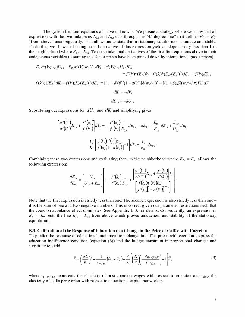
The system has four equations and five unknowns. We pursue a strategy where we show that an expression with the two unknowns E1,t and E0,t cuts through the “45 degree line” that defines E1,t = E0,t “from above” unambiguously. This allows us to state that a stationary equilibrium is unique and stable. To do this, we show that taking a total derivative of this expression yields a slope strictly less than 1 in the neighborhood where E1,t = E0,t. To do so take total derivatives of the first four equations above in their endogenous variables (assuming that factor prices have been pinned down by international goods prices): E0,tπ′(Vt)wudU1,t + E0,tπ″(Vt)wuU1,tdVt + π′(Vt)wuU1,tdE0,t = f″(kt)*(E1,t)kt – f″(kt)*(E1t/(E0,t)2)dE0,t + f′(kt)dE1,t

f′(kt)(1/E0,t)dKt – f′(kt)(Kt/(E0,t)2)dE0,t = [(1 + β)/β][(1 – π(Vt)]d(wu/ws)] – [(1 + β)/β](wu/ws)π(Vt)]dVt

dKt = –dVt

dE1,t = –dU1,t

Substituting out expressions for and and simplifying gives

.

Combining these two expressions and evaluating them in the neighborhood where E1,t = E0,t allows the following expression:

.

Note that the first expression is strictly less than one. The second expression is also strictly less than one – it is the sum of one and two negative numbers. This is correct given our parameter restrictions such that the coercion avoidance effect dominates. See Appendix B.3. for details. Consequently, an expression in E1,t = E0,t cuts the line E1,t = E0,t from above which proves uniqueness and stability of the stationary equilibrium. B.3. Calibration of the Response of Education to a Change in the Price of Coffee with Coercion To predict the response of educational attainment to a change in coffee prices with coercion, express the education indifference condition (equation (6)) and the budget constraint in proportional changes and substitute to yield

(9)

where ε(1–π(V)),V represents the elasticity of post-coercion wages with respect to coercion and εf(k),k the elasticity of skills per worker with respect to educational capital per worker.

7

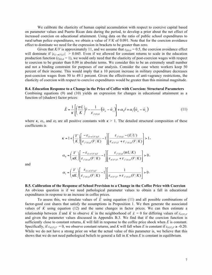
We calibrate the elasticity of human capital accumulation with respect to coercive capital based on parameter values and Puerto Rican data during the period, to develop a prior about the net effect of increased coercion on educational attainment. Using data on the ratio of public school expenditures to rural/urban police expenditures, we obtain a value of V/K of 0.091. Note that for the coercion avoidance effect to dominate we need for the expression in brackets to be greater than zero.

Given that K/V is approximately 11, and we assume that εf(k),k = 0.5, the coercion avoidance effect will dominate if |ε(1–π(V)),V| > 0.045. Even if we allowed for constant returns to scale in the education production function (εf(k),k = 1), we would only need that the elasticity of post-coercion wages with respect to coercion to be greater than 0.09 in absolute terms. We consider this to be an extremely small number and not a binding constraint for purposes of our analysis. Consider the case where workers keep 50 percent of their income. This would imply that a 10 percent increase in military expenditure decreases post-coercion wages from 50 to 49.1 percent. Given the effectiveness of anti-vagrancy restrictions, the elasticity of coercion with respect to coercive expenditures would be greater than this minimal magnitude. B.4. Education Response to a Change in the Price of Coffee with Coercion: Structural Parameters Combining equations (9) and (10) yields an expression for changes in educational attainment as a function of (shadow) factor prices:

(11)

where κ, α1, and α2 are all positive constants with κ > 1. The detailed structural composition of these coefficients is

,

,

and

.

B.5. Calibration of the Response of School Provision to a Change in the Coffee Price with Coercion An obvious question is if we need pathological parameter values to obtain a fall in educational expenditures in response to an increase in coffee prices.

To assess this, we simulate values of using equation (11) and all possible combinations of factor-good cost shares that satisfy the assumptions in Proposition 1. We then generate the associated values of using equation (12) and the same changes in factor prices. We can then estimate a relationship between and to observe in the neighborhood of = 0 for differing values of επ'(V),V and given the parameter values discussed in Appendix B.3. We find that if the coercion function is sufficiently close to constant returns, K will fall in response to the coffee price shock when E is constant. Specifically, if επ'(V),V = 0, we observe constant returns, and K will fall when E is constant if επ'(V),V ≥ -0.20. While we do not have a strong prior on what the actual value of this parameter is, we believe that this shows that we do not need pathological beliefs to general a fall in K when E is constant in equilibrium.

8

Appendix C: Robustness Checks

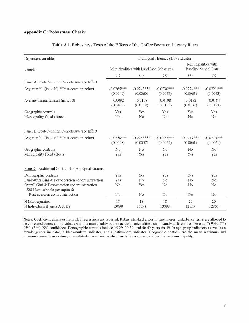
Table A1: Robustness Tests of the Effects of the Coffee Boom on Literacy Rates

Notes: Coefficient estimates from OLS regressions are reported. Robust standard errors in parentheses; disturbance terms are allowed to be correlated across all individuals within a municipality but not across municipalities; significantly different from zero at (*) 90%, (**) 95%, (***) 99% confidence. Demographic controls include 25-29, 30-39, and 40-49 years (in 1910) age group indicators as well as a female gender indicator, a black/mulatto indicator, and a native-born indicator. Geographic controls are the mean maximum and minimum annual temperature, mean altitude, mean land gradient, and distance to nearest port for each municipality.

9

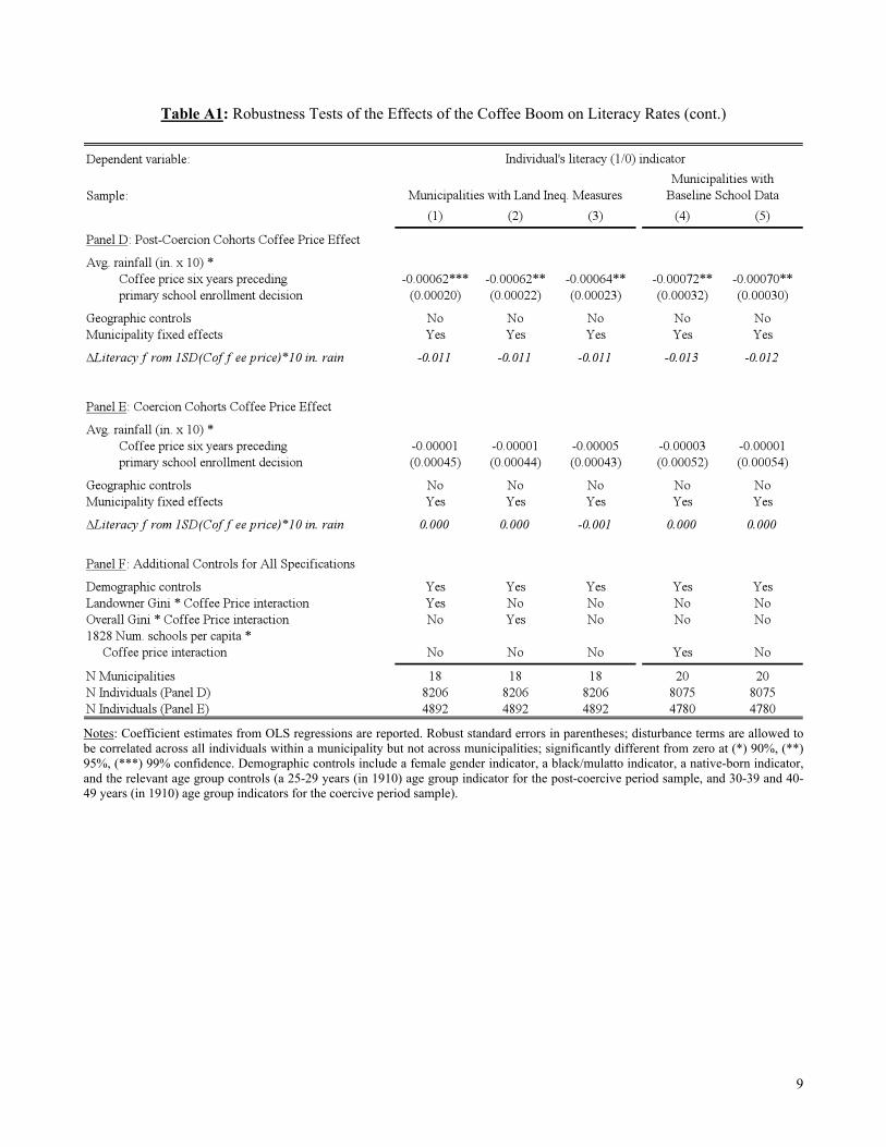
Table A1: Robustness Tests of the Effects of the Coffee Boom on Literacy Rates (cont.)

Notes: Coefficient estimates from OLS regressions are reported. Robust standard errors in parentheses; disturbance terms are allowed to be correlated across all individuals within a municipality but not across municipalities; significantly different from zero at (*) 90%, (**) 95%, (***) 99% confidence. Demographic controls include a female gender indicator, a black/mulatto indicator, a native-born indicator, and the relevant age group controls (a 25-29 years (in 1910) age group indicator for the post-coercive period sample, and 30-39 and 40-49 years (in 1910) age group indicators for the coercive period sample).

10

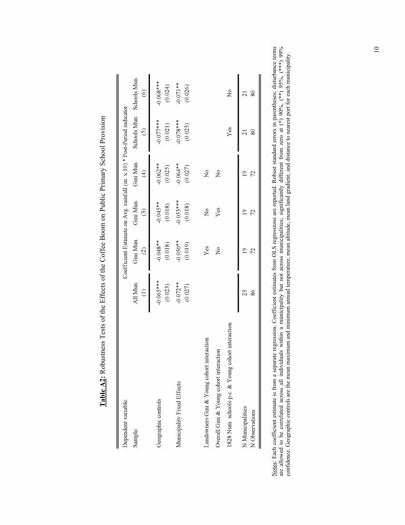
T

able

A2:

Rob

ustn

ess T

ests

of t

he E

ffec

ts o

f the

Cof

fee

Boo

m o

n Pu

blic

Prim

ary

Scho

ol P

rovi

sion

N

otes

: Eac

h co

effic

ient

est

imat

e is

from

a s

epar

ate

regr

essi

on. C

oeff

icie

nt e

stim

ates

from

OLS

regr

essi

ons

are

repo

rted.

Rob

ust s

tand

ard

erro

rs in

par

enth

eses

; dis

turb

ance

term

s ar

e al

low

ed t

o be

cor

rela

ted

acro

ss a

ll in

divi

dual

s w

ithin

a m

unic

ipal

ity b

ut n

ot a

cros

s m

unic

ipal

ities

; si

gnifi

cant

ly d

iffer

ent

from

zer

o at

(*)

90%

, (*

*) 9

5%,

(***

) 99

%

conf

iden

ce. G

eogr

aphi

c co

ntro

ls a

re th

e m

ean

max

imum

and

min

imum

ann

ual t

empe

ratu

re, m

ean

altit

ude,

mea

n la

nd g

radi

ent,

and

dist

ance

to n

eare

st p

ort f

or e

ach

mun

icip

ality

.