One Picture and a Thousand WordsUsing Matrix Approximtions

October 2017Oak Ridge National Lab

Dianne P. O’Learyc©2017

1

One Picture and a Thousand WordsUsing Matrix Approximations

Dianne P. O’Leary

Computer Science Dept. andInstitute for Advanced Computer Studies

University of Maryland

Joint work withJulianne Chung,Matthias Chung,John M. Conroy,

Yi-Kai Liu

Support from NSF.

2

Introduction: The Problem

Given: a rank r matrix A ∈ Rm×n, with m ≥ n,

Determine: an approximation Z of rank k ≤ r.

Low rank approximations of matrices and their inverses play an importantrole in many applications, such as image reconstruction, machine learning,text processing, matrix completion problems, signal processing, optimalcontrol problems, statistics, and mathematical biology.

How we

• measure the goodness f (A,Z) of the approximation, and

• what additional constraints we put on Z

determine how hard our problem is.

How hard can it be?

3

First measure of goodness: Frobenius norm

minrank(Z)≤k

f (A,Z), f (A,Z) = ‖A− Z‖2F

Solution: best rank k approximation Let

A = UΣV>

be the singular value decomposition of A, with U = [u1, . . . ,um] andV = [v1, . . . , vn] and σ1 ≥ σ2 ≥ . . . ≥ σn ≥ 0.

The Eckart-Young Theorem, Schmidt 1907, Eckart and Young 1936,Mirsky 1960 (unitarily invariant norms)

Z = UkΣkV>k

withUk = [u1, . . . ,uk], Vk = [v1, . . . , vk],

Σk = diag(σ1, . . . , σk) .

The solution is unique if and only if σk > σk+1.

4

End of story?

Today we’ll consider two other ways to form low-rank approximations:

• Inverse approximation.Joint work with Julianne Chung and Matthias Chung.

• Interval approximation.Joint work with John M. Conroy and Yi-Kai Liu.

And we’ll discuss why these viewpoints are necessary and useful.

Just as in the Eckart-Young theorem, our approximations take the form

Z = XY, X : m× k,Y : k × n.First we’ll give two examples of why we might want constraints on X andY, not just on Z.

5

This seems odd.

Why put constraints on X and Y when it is Z = XY that is supposed toapproximate A?

6

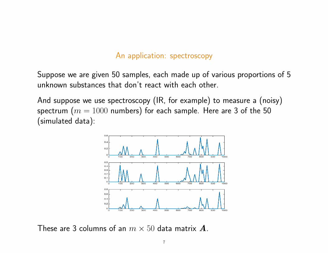
An application: spectroscopy

Suppose we are given 50 samples, each made up of various proportions of 5unknown substances that don’t react with each other.

And suppose we use spectroscopy (IR, for example) to measure a (noisy)spectrum (m = 1000 numbers) for each sample. Here are 3 of the 50(simulated data):

These are 3 columns of an m× 50 data matrix A.

7

Each spectrum measures a response at 1000 frequencies, and they arenonnegative.

We’ve been told that each spectrum ai is of the form

ai = y1ix1 + y2ix2 + y3ix3 + y4ix4 + y5ix5, i = 1, . . . , n

x vectors: the spectra for the five unknown substancesy coefficients: how much of each substance is in the ith sample.

So we want a good approximation Z = XY to the data matrix A, but tomake it physically meaningful, we need both X and Y to be nonnegative.

Also, the vectors X should be sparse, because the spectrum for eachsubstance has a small number of peaks (nonzero responses).

8

Another application: document classification

Suppose we are given 500 documents (e.g., articles from the mathliterature) and we want to classify them into k subjects.

Let’s gather the distinct terms in the documents (‘decomposition’,‘topology’, ’category theory’, ‘derivative’, etc.) and create a matrix A thathas one row for each term.

Set aij to be a measure of the importance of term i in document j, fori = 1, . . . ,m = the number of terms and j = 1, . . . , 500.

If we can determine a nonnegative m× k matrix X and a nonnegativek× 500 matrix Y with A ≈ XY, then each column of A is approximatelya combination of the columns of X. The coefficients in the ith column ofY tell us how important each of these dictionary columns is to document i.

We would expect both X and Y to be nonnegative.

And we would also expect sparsity in each of these matrices.

9

Do we want to approximate a matrix, or its inverse?

10

A different measure of goodness: Inverse approximation

Instead ofmin

rank(Z)≤kf (A,Z), f (A,Z) = ‖A− Z‖2F

let’s consider

minrank(Z)≤k

f (A,Z) f (A,Z) = ‖ZA− In‖2F

A solution:Z = VkΣ

−1k U>k .

But any choice of k nonzero singular values and the corresponding vectorsgives a global minimizer, so the problem is not well-posed.

11

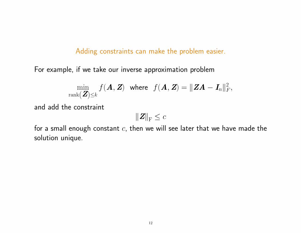
Adding constraints can make the problem easier.

For example, if we take our inverse approximation problem

minrank(Z)≤k

f (A,Z) where f (A,Z) = ‖ZA− In‖2F ,

and add the constraint‖Z‖F ≤ c

for a small enough constant c, then we will see later that we have made thesolution unique.

12

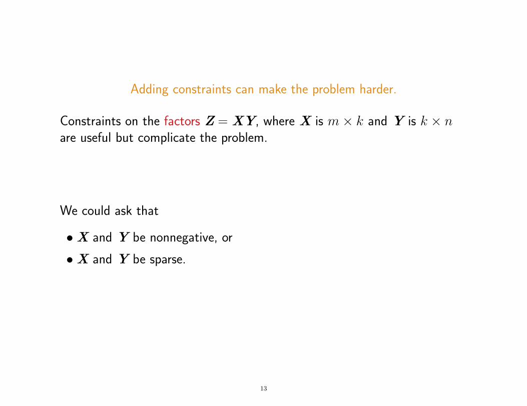
Adding constraints can make the problem harder.

Constraints on the factors Z = XY, where X is m× k and Y is k × nare useful but complicate the problem.

We could ask that

•X and Y be nonnegative, or

•X and Y be sparse.

13

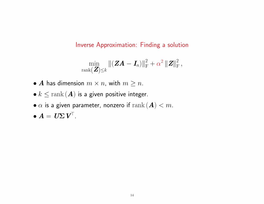
Inverse Approximation: Finding a solution

minrank(Z)≤k

‖(ZA− In)‖2F + α2 ‖Z‖2F ,

•A has dimension m× n, with m ≥ n.

• k ≤ rank (A) is a given positive integer.

• α is a given parameter, nonzero if rank (A) < m.

•A = UΣV>.

14

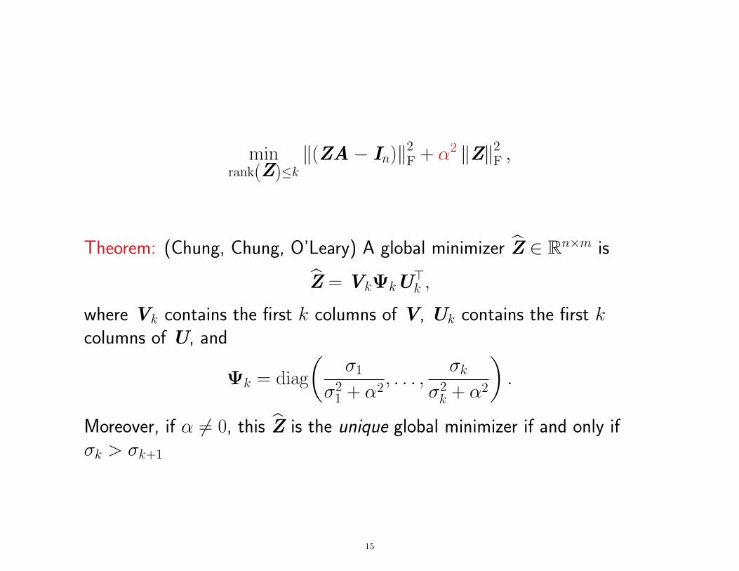
minrank(Z)≤k

‖(ZA− In)‖2F + α2 ‖Z‖2F ,

Theorem: (Chung, Chung, O’Leary) A global minimizer Z ∈ Rn×m is

Z = VkΨkU>k ,

where Vk contains the first k columns of V, Uk contains the first kcolumns of U, and

Ψk = diag

(σ1

σ21 + α2, . . . ,

σkσ2k + α2

).

Moreover, if α 6= 0, this Z is the unique global minimizer if and only ifσk > σk+1

15

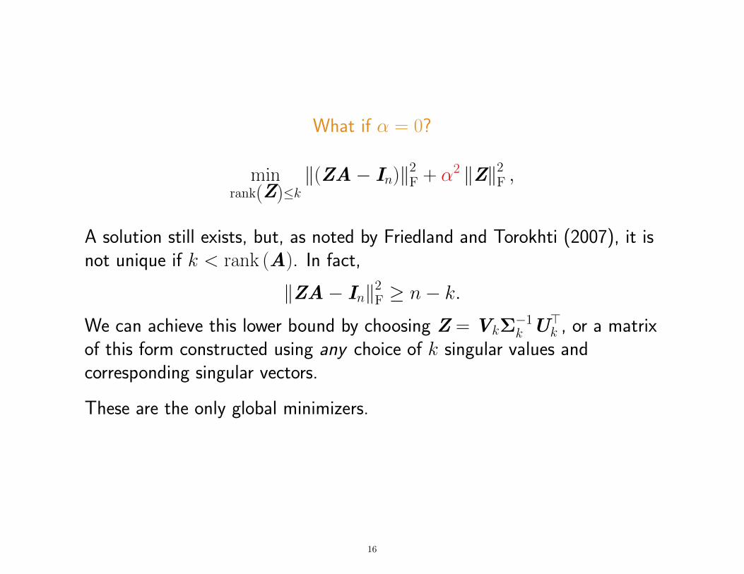
What if α = 0?

minrank(Z)≤k

‖(ZA− In)‖2F + α2 ‖Z‖2F ,

A solution still exists, but, as noted by Friedland and Torokhti (2007), it isnot unique if k < rank (A). In fact,

‖ZA− In‖2F ≥ n− k.We can achieve this lower bound by choosing Z = VkΣ

−1k U>k , or a matrix

of this form constructed using any choice of k singular values andcorresponding singular vectors.

These are the only global minimizers.

16

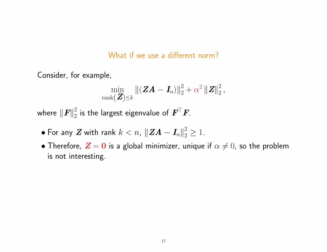
What if we use a different norm?

Consider, for example,

minrank(Z)≤k

‖(ZA− In)‖22 + α2 ‖Z‖22 ,

where ‖F‖22 is the largest eigenvalue of F>F.

• For any Z with rank k < n, ‖ZA− In‖22 ≥ 1.

• Therefore, Z = 0 is a global minimizer, unique if α 6= 0, so the problemis not interesting.

17

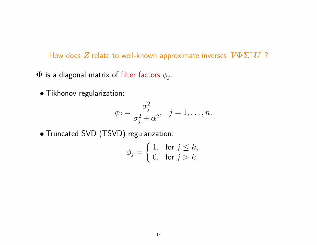
How does Z relate to well-known approximate inverses VΦΣ†U>?

Φ is a diagonal matrix of filter factors φj.

• Tikhonov regularization:

φj =σ2j

σ2j + α2, j = 1, . . . , n.

• Truncated SVD (TSVD) regularization:

φj =

{1, for j ≤ k,0, for j > k.

18

How does Z relate to well-known approximate inverses VΦΣ†U>?

Φ is a diagonal matrix of filter factors φj.

• Tikhonov regularization:

φj =σ2j

σ2j + α2, j = 1, . . . , n.

• Truncated SVD (TSVD) regularization:

φj =

{1, for j ≤ k,0, for j > k.

• Our approximate inverse: Truncated Tikhonov regularization

φj =

σ2jσ2j+α

2 , for j ≤ k,

0, for j > k.

19

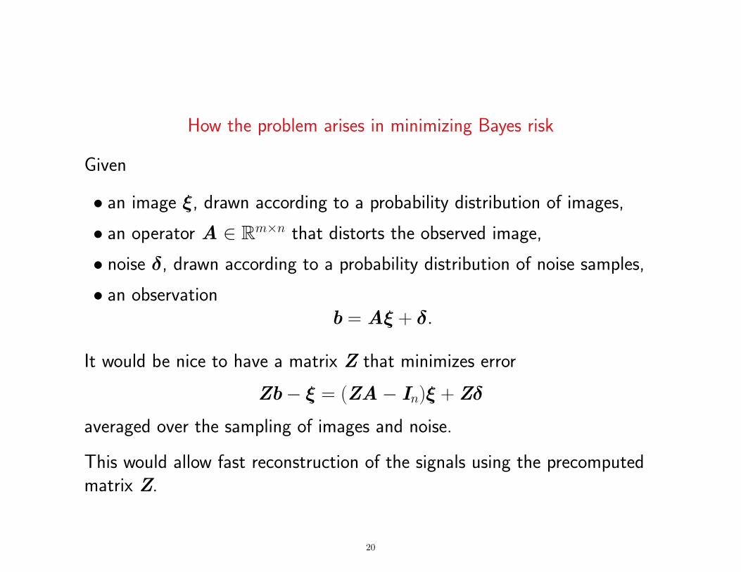
How the problem arises in minimizing Bayes risk

Given

• an image ξ, drawn according to a probability distribution of images,

• an operator A ∈ Rm×n that distorts the observed image,

• noise δ, drawn according to a probability distribution of noise samples,

• an observationb = Aξ + δ.

It would be nice to have a matrix Z that minimizes error

Zb− ξ = (ZA− In)ξ + Zδ

averaged over the sampling of images and noise.

This would allow fast reconstruction of the signals using the precomputedmatrix Z.

20

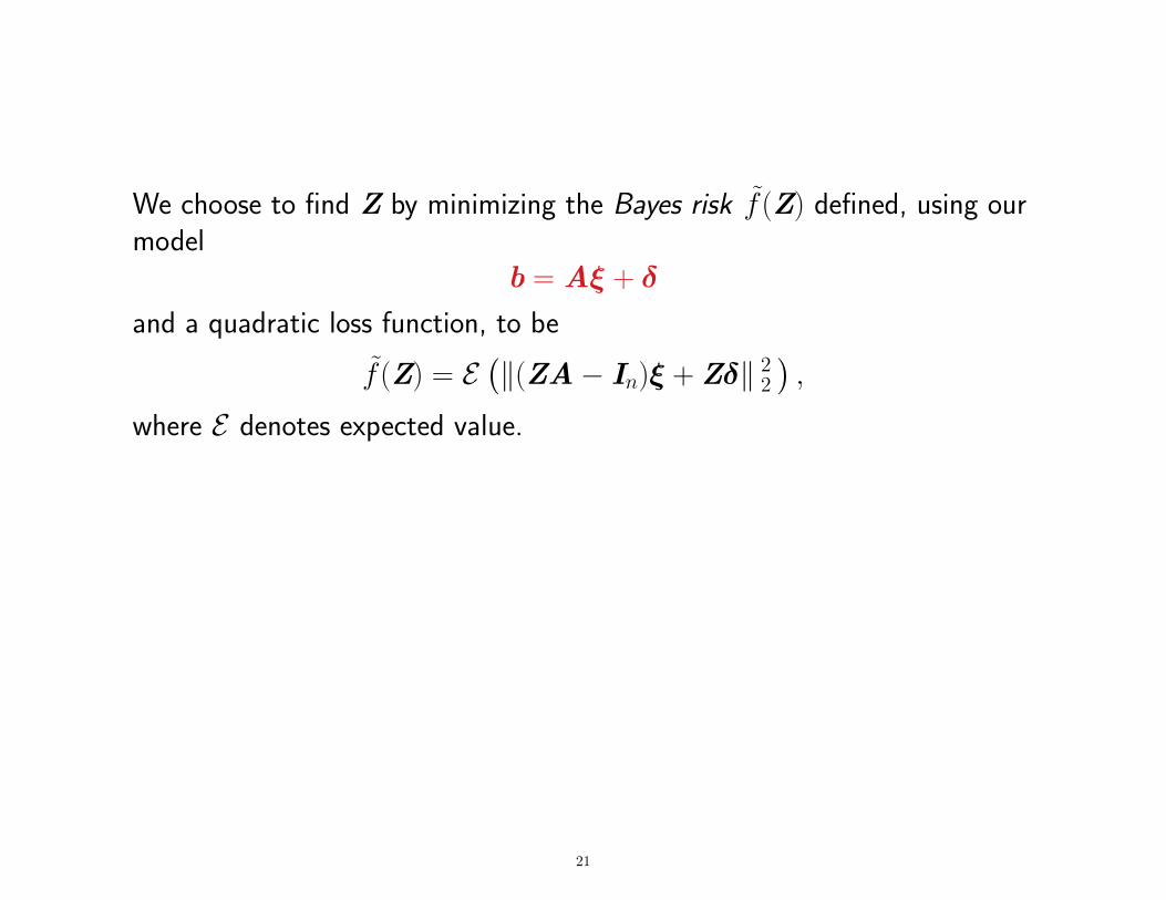
We choose to find Z by minimizing the Bayes risk f (Z) defined, using ourmodel

b = Aξ + δ

and a quadratic loss function, to be

f (Z) = E(‖(ZA− In)ξ + Zδ‖ 2

2

),

where E denotes expected value.

21

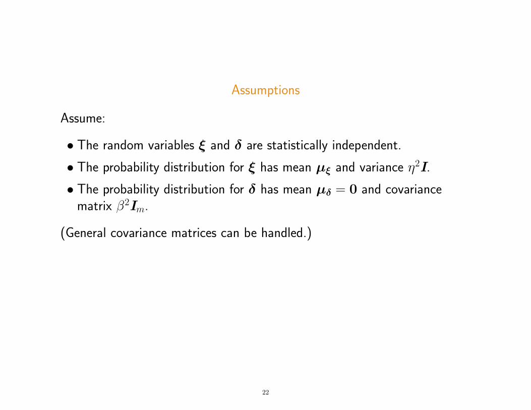
Assumptions

Assume:

• The random variables ξ and δ are statistically independent.

• The probability distribution for ξ has mean µξ and variance η2I.

• The probability distribution for δ has mean µδ = 0 and covariancematrix β2Im.

(General covariance matrices can be handled.)

22

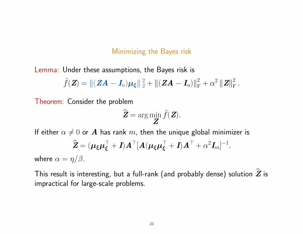
Minimizing the Bayes risk

Lemma: Under these assumptions, the Bayes risk is

f (Z) = ‖(ZA− In)µξ‖ 22 + ‖(ZA− In)‖2F + α2 ‖Z‖2F .

Theorem: Consider the problem

Z = argminZ

f (Z).

If either α 6= 0 or A has rank m, then the unique global minimizer is

Z = (µξµ>ξ + I)A>[A(µξµ

>ξ + I)A> + α2Im]

−1.

where α = η/β.

This result is interesting, but a full-rank (and probably dense) solution Z isimpractical for large-scale problems.

23

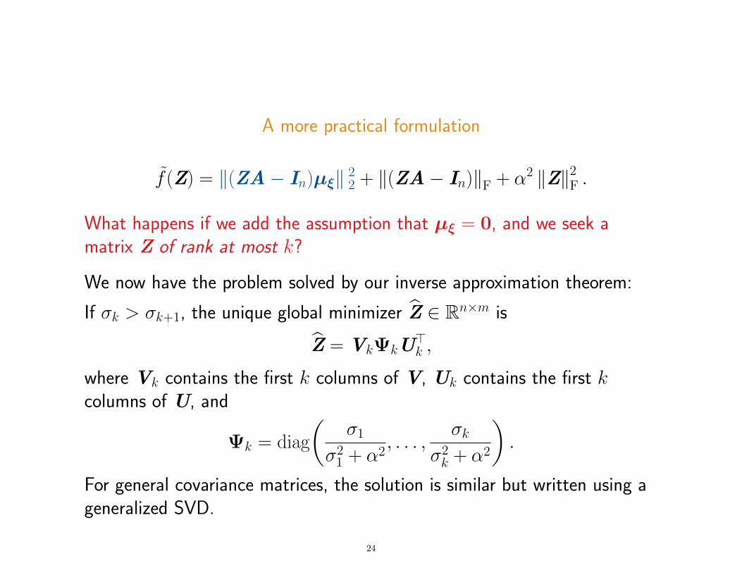
A more practical formulation

f (Z) = ‖(ZA− In)µξ‖ 22 + ‖(ZA− In)‖F + α2 ‖Z‖2F .

What happens if we add the assumption that µξ = 0, and we seek amatrix Z of rank at most k?

We now have the problem solved by our inverse approximation theorem:

If σk > σk+1, the unique global minimizer Z ∈ Rn×m is

Z = VkΨkU>k ,

where Vk contains the first k columns of V, Uk contains the first kcolumns of U, and

Ψk = diag

(σ1

σ21 + α2, . . . ,

σkσ2k + α2

).

For general covariance matrices, the solution is similar but written using ageneralized SVD.

24

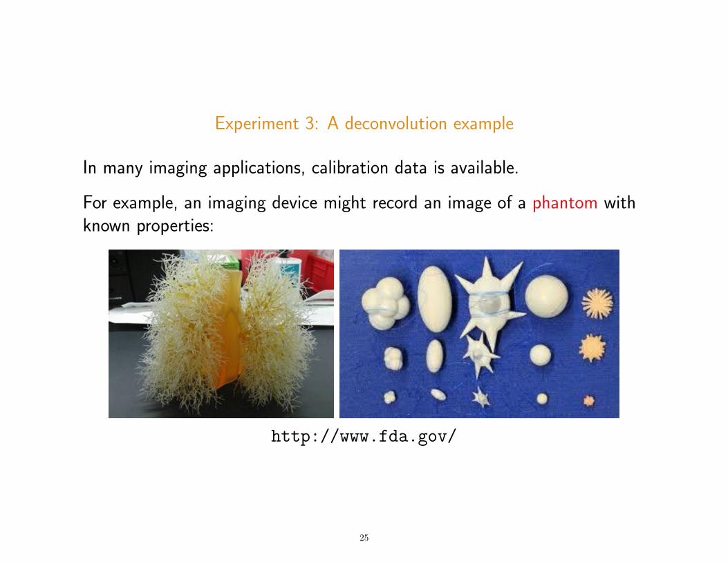
Experiment 3: A deconvolution example

In many imaging applications, calibration data is available.

For example, an imaging device might record an image of a phantom withknown properties:

http://www.fda.gov/

25

Our calibration data

•We use columns from images above to compute a sample covariancematrix.

•We construct our approximate inverse.

•We use columns from images below to evaluate how well it behaves.

26

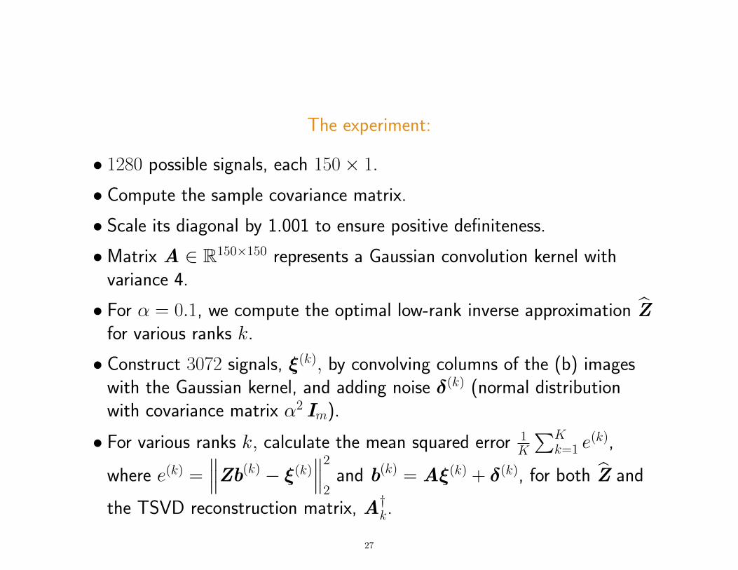
The experiment:

• 1280 possible signals, each 150× 1.

• Compute the sample covariance matrix.

• Scale its diagonal by 1.001 to ensure positive definiteness.

•Matrix A ∈ R150×150 represents a Gaussian convolution kernel withvariance 4.

• For α = 0.1, we compute the optimal low-rank inverse approximation Zfor various ranks k.

• Construct 3072 signals, ξ(k), by convolving columns of the (b) imageswith the Gaussian kernel, and adding noise δ(k) (normal distributionwith covariance matrix α2 Im).

• For various ranks k, calculate the mean squared error 1K

∑Kk=1 e

(k),

where e(k) =∥∥∥Zb(k) − ξ(k)

∥∥∥2

2and b(k) = Aξ(k) + δ(k), for both Z and

the TSVD reconstruction matrix, A†k.

27

5 10 15 20 25 30 35 40 45 50 55 60

100

101

rank J

Mea

nSquare

dE

rror

!ZTSVD

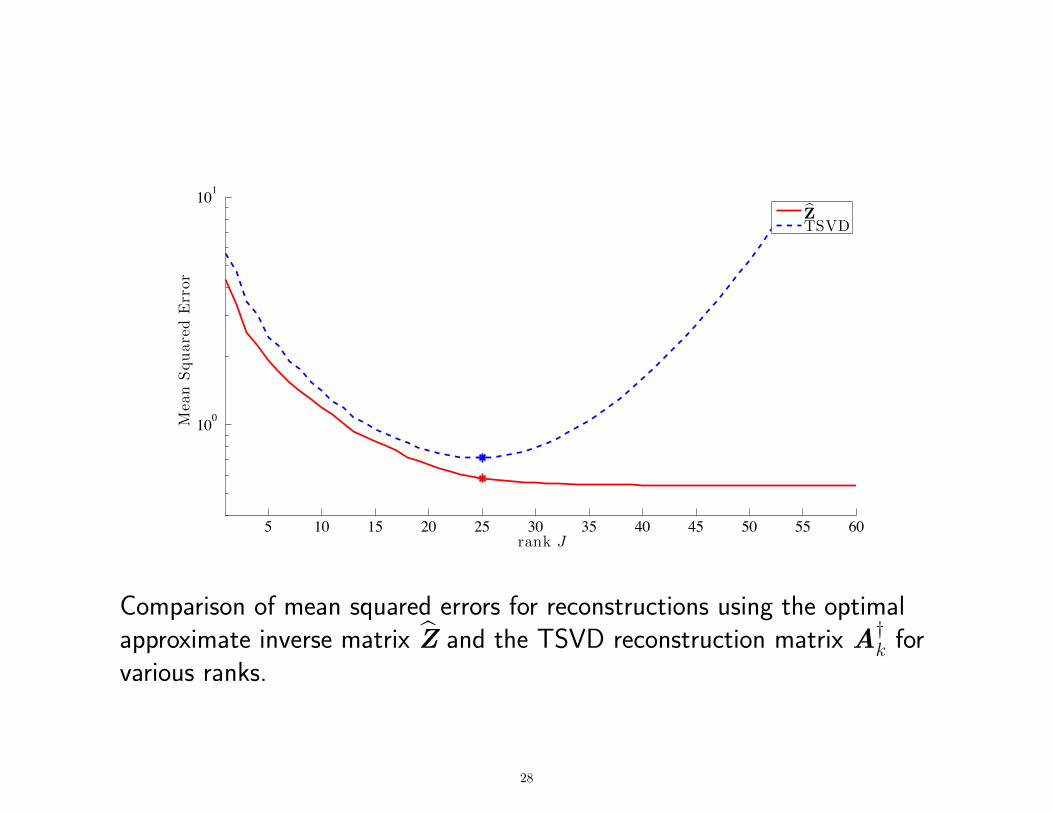
Comparison of mean squared errors for reconstructions using the optimalapproximate inverse matrix Z and the TSVD reconstruction matrix A†k forvarious ranks.

28

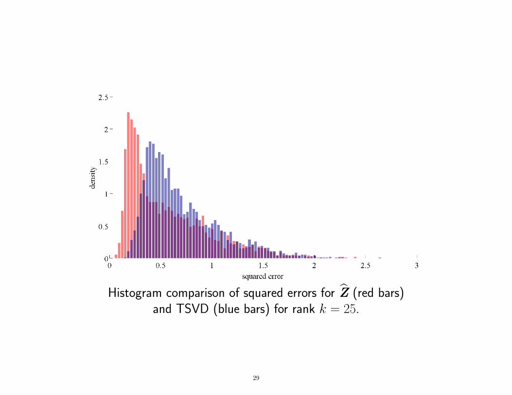
Histogram comparison of squared errors for Z (red bars)and TSVD (blue bars) for rank k = 25.

29

Summary: so far

•We can calculate low-rank approximations to matrix (pseudo)inverses.

• These approximations give us useful reconstructions of images blurredby measurement.

30

Interval approximation

31

We have discussed some great ways to approximate matrices...

... very useful for the particular situations above.

But sometimes noise is quite abnormal.

Often our data matrix A stores counts.

We might count more or less than the true value, but we can never get anegative count.

32

An alternative framework

What if we have an uncertainty interval for each matrix element? Wewould be given matrices L and U satisfying

L ≤ Atrue ≤ U,

where Atrue is unknown.

•We can explicitly impose a nonnegativity assumption, choosing L ≥ 0.

•We can easily accommodate different uncertainties in different matrixelements.

•We can even accommodate missing observations by setting elements ofL to zero and elements of U to +∞.

• Our original formulation is a special case, with L = U.

33

Our problem becomesmin

X,Y,Zf (XY− Z)

` ≤ z ≤ u,

For f , any matrix norm can be used, and we can also include a weightmatrix W if we care more about keeping some particular elements withintheir bounds.

34

So far, our problem is ill-posed.

If XY = Z solve the problem,

then (for example) so do γX, γ−1Y,Z for any positive γ.

35

Added constraints

•We add constraints:

X ≥ 0 and Y ≥ 0.

Still ill-posed.

• It is also useful to add terms to the minimization function to“encourage” sparsity in the factors:

eTx + eTy.

Now the γ non-uniqueness goes away.

BUT the sparsest X and Y are the zero matrices, so we can’t weightthese terms too heavily without risking a rank-deficient solution to ourproblem.

So to balance these terms, we also can include these:

− log det(XTX)− log det(YYT ).

36

log det is scary!

F (X) = − log det(XTX),

http://pumpkinstencils.org/

37

• Both XTX and YYT are small (5× 5 or 50× 50 in our examples, soevaluation is inexpensive.

• The partial derivatives of F (X), arranged as a matrix, are2X(XTX)−1, so F (X) and its gradient are easily calculated using(compact) QR factorization of X.

• The Hessian matrix with respect to entries in each row of X is also easyto calculate given the (compact) QR factors.

http://pumpkinstencils.org/

38

Z is scary!

Up until now, we have had only k(m + n) variables.

But Z adds mn more!!

39

Z is scary!

Really, really scary!Up until now, we have had only k(m + n) variables.

But Z adds mn more!!

40

Fortunately, I can tell you an optimal choice of Z for any given X and Y:

zij(X,Y) =

`ij, (XY)ij ≤ `ij(XY)ij, `ij ≤ (XY)ij ≤ uij,uij, uij ≤ (XY)ij.

So algorithms that alternate updating X and updating Y can be used, andwe update Z using this formula.

41

Alternating algorithms

minX,Y,Z

‖XY−Z‖2F+α1eTx + α2e

Ty−α3(log det(XTX)− log det(YYT ))

Repeat

Update X.Determine the optimal Z based on the current X and Y.Update Y.Determine the optimal Z based on the current X and Y.

Until convergence.

• Blue steps: not seen in previous algorithms, because now L 6= U.

• Red steps: various choices in the literature.

42

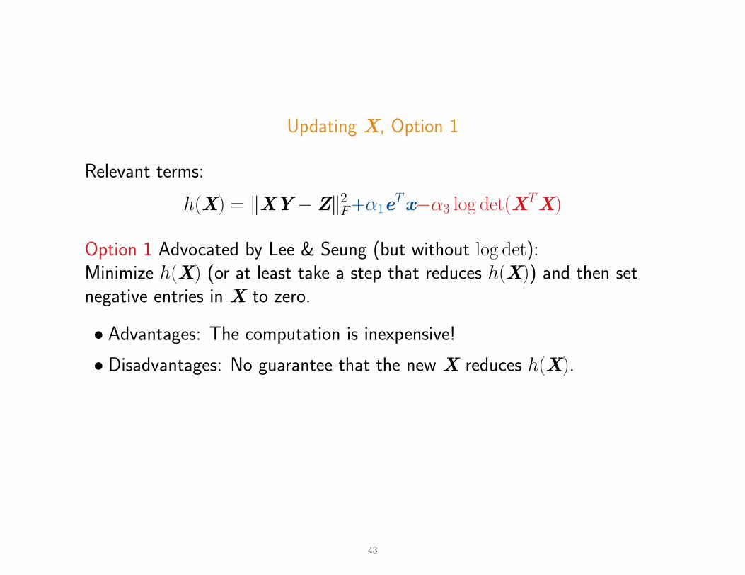
Updating X, Option 1

Relevant terms:

h(X) = ‖XY− Z‖2F+α1eTx−α3 log det(X

TX)

Option 1 Advocated by Lee & Seung (but without log det):Minimize h(X) (or at least take a step that reduces h(X)) and then setnegative entries in X to zero.

• Advantages: The computation is inexpensive!

• Disadvantages: No guarantee that the new X reduces h(X).

43

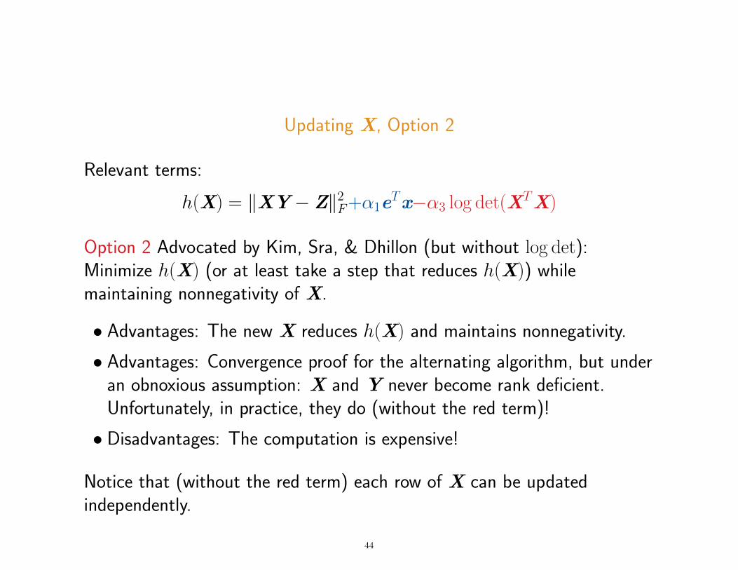
Updating X, Option 2

Relevant terms:

h(X) = ‖XY− Z‖2F+α1eTx−α3 log det(X

TX)

Option 2 Advocated by Kim, Sra, & Dhillon (but without log det):Minimize h(X) (or at least take a step that reduces h(X)) whilemaintaining nonnegativity of X.

• Advantages: The new X reduces h(X) and maintains nonnegativity.

• Advantages: Convergence proof for the alternating algorithm, but underan obnoxious assumption: X and Y never become rank deficient.Unfortunately, in practice, they do (without the red term)!

• Disadvantages: The computation is expensive!

Notice that (without the red term) each row of X can be updatedindependently.

44

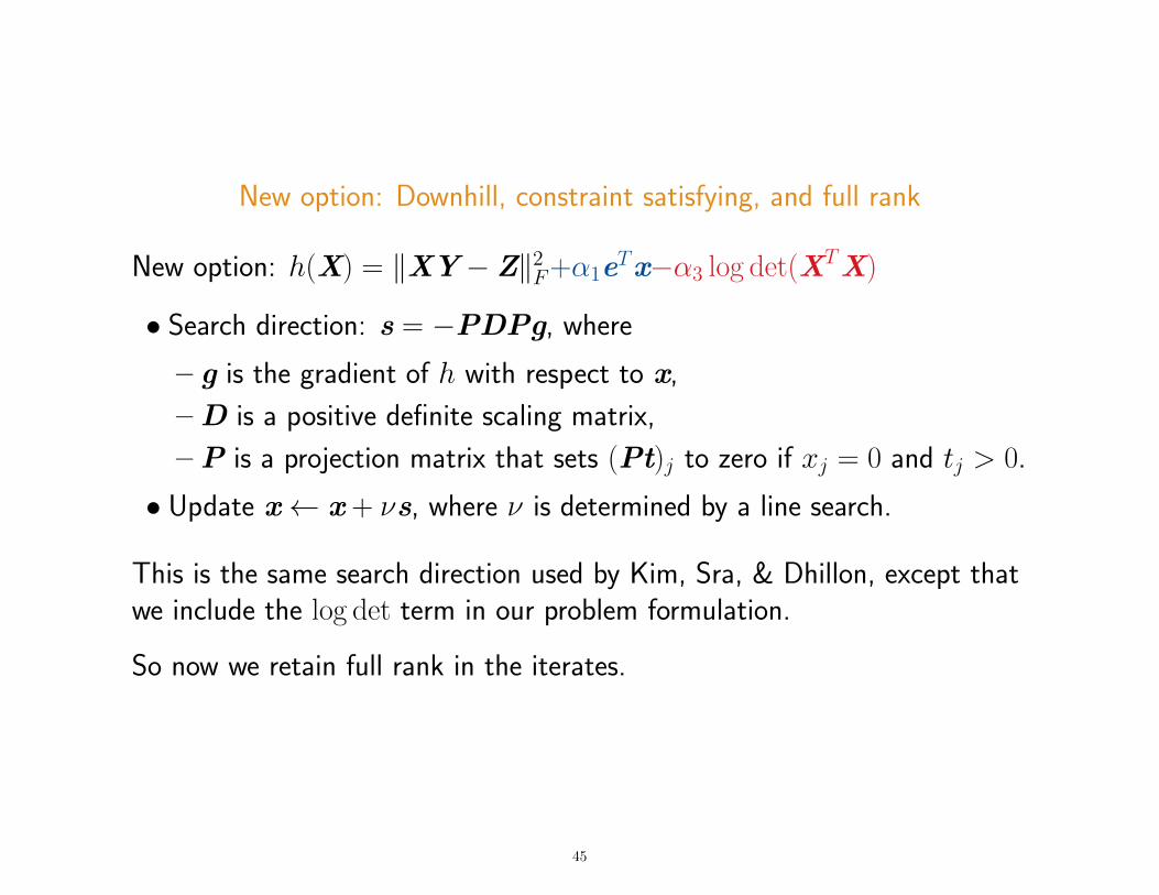
New option: Downhill, constraint satisfying, and full rank

New option: h(X) = ‖XY− Z‖2F+α1eTx−α3 log det(X

TX)

• Search direction: s = −PDPg, where

– g is the gradient of h with respect to x,

– D is a positive definite scaling matrix,

– P is a projection matrix that sets (Pt)j to zero if xj = 0 and tj > 0.

• Update x← x + νs, where ν is determined by a line search.

This is the same search direction used by Kim, Sra, & Dhillon, except thatwe include the log det term in our problem formulation.

So now we retain full rank in the iterates.

45

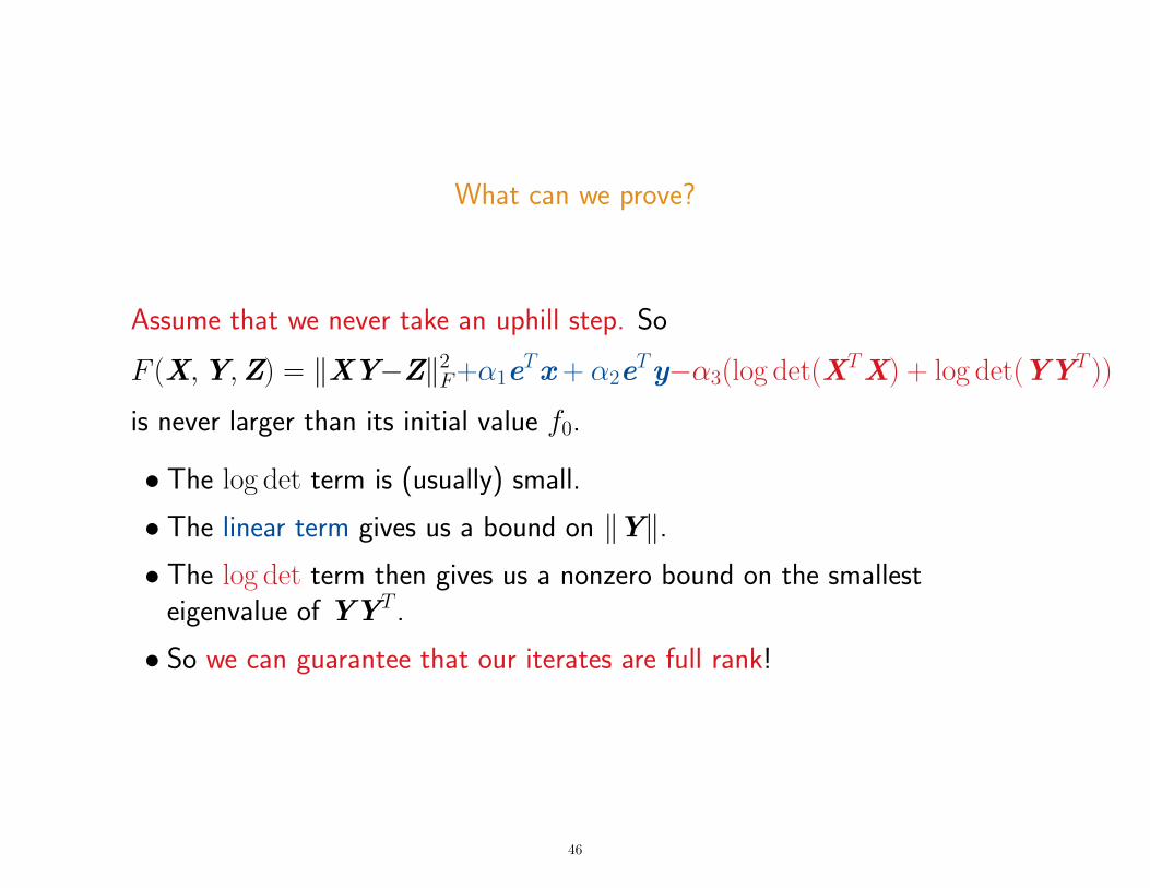
What can we prove?

Assume that we never take an uphill step. So

F (X,Y,Z) = ‖XY−Z‖2F+α1eTx + α2e

Ty−α3(log det(XTX) + log det(YYT ))

is never larger than its initial value f0.

• The log det term is (usually) small.

• The linear term gives us a bound on ‖Y‖.• The log det term then gives us a nonzero bound on the smallest

eigenvalue of YYT .

• So we can guarantee that our iterates are full rank!

46

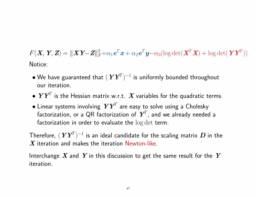
F (X,Y,Z) = ‖XY−Z‖2F+α1eTx + α2e

Ty−α3(log det(XTX) + log det(YYT ))

Notice:

•We have guaranteed that (YYT )−1 is uniformly bounded throughoutour iteration.

•YYT is the Hessian matrix w.r.t. X variables for the quadratic terms.

• Linear systems involving YYT are easy to solve using a Choleskyfactorization, or a QR factorization of YT , and we already needed afactorization in order to evaluate the log det term.

Therefore, (YYT )−1 is an ideal candidate for the scaling matrix D in theX iteration and makes the iteration Newton-like.

Interchange X and Y in this discussion to get the same result for the Yiteration.

47

Results: Document classification

DUC 2004 data: Term-document matrix for 500 documents (some repeats)that are “correctly” classified in 50 classes of 10 documents each.

Measures of correctness: LetA = number of agreements: document i and j in same/different classD = number of disagreements,so that A+D = comb(n,2). Then

.9846 = RI = Rand index (1971) = A / comb(n,2) = prob agree

.9692 = HI = Hubert index (1977) = (A - D) / comb(n,2) = RI - MI

.6252 = AR = adjusted RI, corrected for chance Hubert+Arabie (1985)

.7500 = AMI = adjusted mutual index

Comparable to competing methods.

48

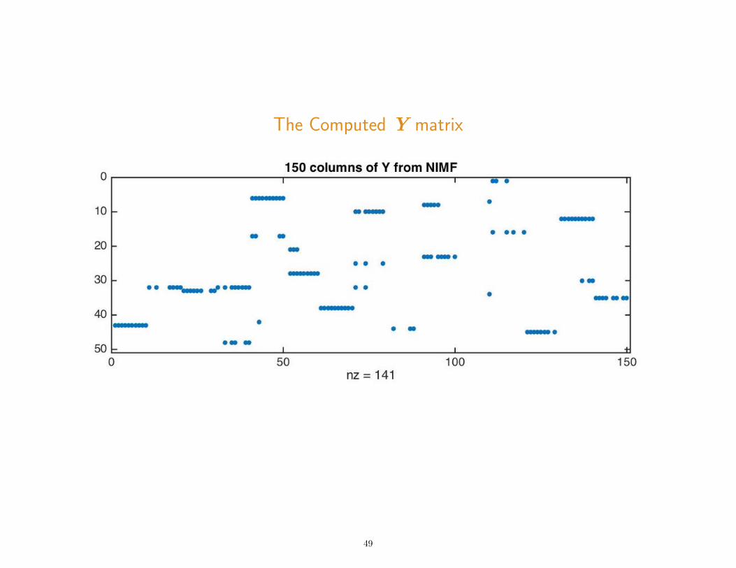
The Computed Y matrix

49

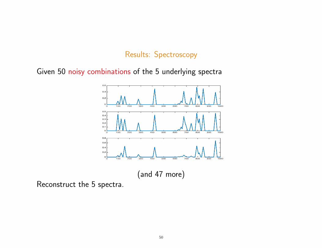
Results: Spectroscopy

Given 50 noisy combinations of the 5 underlying spectra

(and 47 more)Reconstruct the 5 spectra.

50

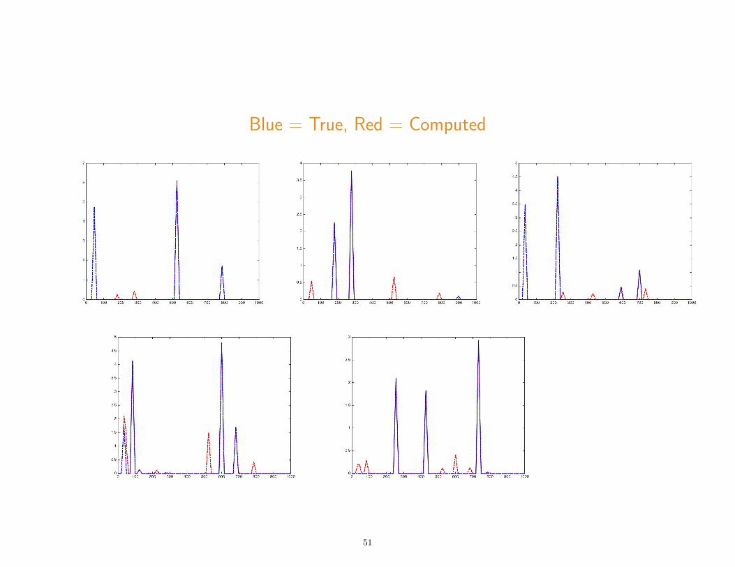
Blue = True, Red = Computed

51

Conclusions

A fresh look at low-rank matrix approximation is productive and useful!

• Inverse Approximation of Matrices

– We can calculate low-rank approximations to matrix (pseudo)inverses.

– These approximations give us useful reconstructions of images blurredby measurement when calibration data is available.

• Approximation of Interval Matrices

– We have a new formulation of matrix approximation that allows errorbounds and weights on each matrix entry.

– We have a descent algorithm that takes Newton-like steps to improvethe free variables.

– We have demonstrated promising results for document classificationand signal recovery.

52

References for Inverse Approximation:

• Julianne Chung, Matthias Chung, and Dianne P. O’Leary“Optimal Regularized Low-Rank Inverse Approximation,” Linear Algebraand Its Applications, 468(1) (2015) 260-269.

• Julianne M. Chung, Matthias Chung, and Dianne P. O’Leary, ”OptimalFilters from Calibration Data for Image Deconvolution with DataAcquisition Errors,” Journal of Mathematical Imaging and Vision, 44(3),pp. 366–374 (2012)

53

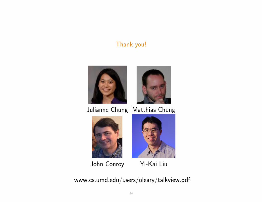
Thank you!

Julianne Chung Matthias Chung

John Conroy Yi-Kai Liu

www.cs.umd.edu/users/oleary/talkview.pdf

54