Embed Size (px)
Citation preview

On the Use of Discrete Prolate Spheroidal Windows for Frequency Selective Filter Design
Lav Varshney
Applications of Signal Processing School of Electrical and Computer Engineering
Cornell University February 23, 2004
Abstract—The FIR filter design problem is considered with respect to a combined integrated squared error-Chebyshev error criterion. Truncation of the DTFT of the desired frequency response with tapered windows is introduced and the discrete prolate spheroidal window is shown to be a good window for this purpose, due to its optimal mainlobe width-sidelobe energy tradeoff. The discrete prolate spheroidal window is shown to be a scalar multiple of the zero-order discrete prolate spheroidal sequence, and a commutable matrix reformulation for numerically well-conditioned computation is given. Discrete prolate spheroidal window parameters are related to frequency selective filter parameters through empirical study. Integrated squared error-Chebyshev error tradeoffs for filters designed with discrete prolate spheroidal windows are compared with other window methods, with the optimal constrained least squares method, and with the optimal Chebyshev method. It is found that the discrete prolate spheroidal window method is suboptimal, but is best among window methods. Finally, a suggestion for the use of discrete prolate spheroidal windows for spectral analysis is provided. MATLAB code is included in the appendices.
I. Introduction Filter design is fundamentally a problem of finding a practical, realizable filter that
approximates an ideal, desired filter. Frequency domain methods of filter design attempt to minimize the difference between the desired frequency response and the actual frequency response, with respect to an error criterion. If one considers the causal, linear phase, finite impulse response, frequency selective filter design problem, the desired passband frequency response will be e-jωτ, for some constant τ, and the desired stopband frequency response will be 0, with discontinuities at the boundaries between bands.
The optimal least squares filter can be found by simply truncating the discrete-time Fourier transform (DTFT) of the ideal frequency response. Maintenance of linear phase requires truncation with preservation of symmetry in the unit pulse response. Optimality of the filter with regard to the integrated squared error criterion is guaranteed by the orthogonality principle. Due to the nonuniform convergence of the truncated response, the optimal least squares filter suffers from the Gibbs phenomenon. This phenomenon manifests itself in the frequency domain as a convolution between the ideal rectangular frequency response and the Dirichlet (periodic sinc) function, the DTFT of the rectangular truncation.
For many applications of frequency-selective filters, the large amplitude ripples introduced by Gibbs phenomenon are objectionable, since they may introduce amplitude distortion in the passband and may allow strong single frequency interferers in the stopband to pass without sufficient attenuation. Thus it is seen that the integrated squared error criterion is often not the natural criterion for optimization. Determination of a suitable error criterion for filter design has been a subject of considerable debate. In a humorous1 correspondence article from the 1950s, Ernst A. Guillemin commented that everyone seemed to take for granted that the integrated squared error criterion is also nature’s error criterion, but that other error criterion such as the Chebyshev maximum error criterion may be more suitable [1].
The optimal Chebyshev filter, the filter that minimizes maximum error over all frequency bands, is an equiripple filter and can be found with the Parks-McClellan algorithm. The Parks-McClellan algorithm formulates the filter design problem as a problem in polynomial approximation and uses Remez exchange to find the optimal filter. The design algorithm disallows the use of adjacent frequency bands in the desired frequency response so as to use the alternation theorem to recognize the optimal solution. Therefore a “transition region” must be introduced in the desired frequency response, altering the approximation problem, and often adversely affecting the result for applications in which there is no natural transition region. Furthermore, the optimal Chebyshev filters have large integrated squared error, and so are also considered suboptimal for many applications of frequency-selective filters. Thus Chebyshev
1 Guillemin describes [1] as “light and fluffy with a bit of humor and fun thrown in” [2].

error is also not the natural criterion for optimization for many applications. In fact, many applications of frequency-selective filters require a tradeoff between the two error criteria.
II. The Compromise Between Integrated Squared Error and Chebyshev Error
Many techniques have been proposed for designing filters that have good integrated squared error and Chebyshev error performance, that is to say, filter design techniques that consider an error criterion that is a function of the two standard error metrics.
Traditional ways to make the tradeoff between integrated squared error and Chebyshev error are based on reducing Gibbs phenomenon in the optimal least squares filter design. Remember that Gibbs phenomenon is the cause of large Chebyshev errors in optimal least squares filters. One method to reduce Gibbs phenomenon in optimum least squares filters is to modify the desired response by replacing the sharp cutoff with a gradual transition. Gradually decreasing trigonometric and polynomial transition functions have been suggested to replace the discontinuity. Another method is to modify the desired response by introducing “don’t care” transition bands. The error function is given zero weight in these frequency bands. Equivalently, one can consider the support of the error function not to include the transition bands. Thus when the filter is optimized for the integrated squared error criterion, only the passband and stopband are considered, and the result is generally a reduction in maximum error. In general, the sharp cutoffs are smoothed as a result of transition bands [3]. Both of these methods change the original approximation problem to one, which is believed to result in better combined integrated squared-Chebyshev performance.
Constrained least squares filter design is another method for achieving a tradeoff between the squared error and the maximum error. This method designs the optimal least squares filter under the constraint of fixed maximum Chebyshev error. It can produce a wide range of filters that reflect choices made in the least squares-Chebyshev error tradeoff. The design technique employs an exchange algorithm that uses Langrage multipliers and Kuhn-Tucker conditions on each iteration [4].
An additional method to make a tradeoff between integrated squared error and Chebyshev error has been to use nonrectangular, smoothly tapering windows to truncate the DTFT of the desired frequency response. The tapered windows serve to reduce Gibbs phenomenon, the cause of large Chebyshev errors in optimal least squares filters. Many types of window functions have been proposed for the design of frequency selective filters. The use of parameterized families of window functions allow a continuum of filters to be designed. Examples include the cosine-on-pedestal family, which includes the Hamming and Hanning windows; the Gaussian or Weierstrass family; the Dolph-Chebyshev family; and the Kaiser family [5],[6].
III. Selection of a Window Family for Filter Design A general window used for filter design is a finite-extent, symmetric, discrete-time
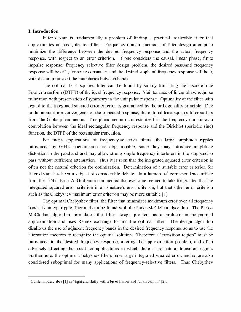
sequence that generally displays tapering at the edges. The DTFT of such a discrete-time sequence displays a mainlobe and smaller sidelobes, which arise due to the finite truncation. Note that the DTFT of a rectangular window is the Dirichlet function (periodic sinc), with a mainlobe and sidelobes, and that the DTFT of a general window is the convolution of some function with this Dirichlet function. Figure 1 shows a time-domain rectangle sequence, the corresponding frequency domain response (the Dirichlet function), and the Dirichlet function on a relative decibel scale. Figure 2 shows the Hamming window, one of the most simple window functions, and a member of the cosine-on-pedestal family. As can be seen, the mainlobe of the Hamming window, like all general window functions is wider than the rectangular window, but that the sidelobe levels are lower.
-10 -5 0 5 100
0.2
0.4
0.6
0.8
1
0 0.05 0.1 0.15 0.2 0.25 0.3 0.35 0.4 0.45 0.5
2
4
6
8
10
12
14
16
18
20
(a) (b)
0 0.05 0.1 0.15 0.2 0.25 0.3 0.35 0.4 0.45-60
-50
-40
-30
-20
-10
0
(c)
Figure 1. The Rectangular Window. (a) time-domain response (b) frequency domain response magnitude (c) frequency domain response magnitude on relative decibel scale.

-10 -5 0 5 100
0.2
0.4
0.6
0.8
1
0 0.05 0.1 0.15 0.2 0.25 0.3 0.35 0.4 0.45 0.5
1
2
3
4
5
6
7
8
9
10
(a) (b)
0 0.05 0.1 0.15 0.2 0.25 0.3 0.35 0.4 0.45 0.5-60
-50
-40
-30
-20
-10
0
(c)
Figure 2. The Hamming Window. (a) time-domain response (b) frequency domain response magnitude (c) frequency domain response magnitude on relative decibel scale.
Windows with smaller sidelobes yield better approximations, in terms of Chebyshev
error, of the ideal response at a discontinuity. This can be seen, since the application of a window involves convolving the ideal frequency response with the frequency of the window, the smaller the sidelobes, the smaller the resulting ripples in the designed filter. The mainlobe width of a window is related to the transition width of the designed filter. Figure 3 shows the definitions for ripple and transition width for a filter.
Desirable windows for filter design can be determined by optimizing the tradeoff between mainlobe width and sidelobe area. The window function that achieves this optimal tradeoff is maximally concentrated around zero frequency in the frequency domain [5]. The Kaiser family of window functions has received particular attention due to the near-optimal tradeoff between mainlobe width and sidelobe area [5],[7], however, discrete prolate spheroidal windows (DPSW) have the optimal energy concentration at low frequencies, and thus may be considered the most desirable for use as filter design windows.

0 0.05 0.1 0.15 0.2 0.25 0.3 0.35 0.4 0.45 0.5
0
0.2
0.4
0.6
0.8
1
1+ δδδδP
1- δδδδP
1+ δδδδS
∆∆∆∆ωωωω
ωωωωC
Figure 3. Definition of Passband Ripple (δP), Stopband Ripple (δS), and Transition Width (∆ω) for a Lowpass Filter. Dash-dot line shows ideal lowpass filter with cutoff ωC and solid line shows magnitude of filter frequency response.
IV. Prolate Spheroidal Wave Functions and Discrete Prolate Spheroidal Sequences
The continuous time problem of maximally concentrating a time-limited function to a limited bandwidth was considered by Slepian, Pollak, and Landau and they found that the prolate spheroidal wave functions (PSWF) are maximally concentrated in this regard [8]-[11].2 Due to the difficulty in computing PSWFs, Kaiser introduced an approximation with I0-sinh functions that use modified Bessel functions of the first kind and zeroth order [7]. Kaiser windows are in fact generated by sampling this I0-sinh approximation.
The discrete-time equivalent to the continuous time problem is determining the extent to which a finite-extent discrete-time sequence can have its spectrum concentrated on an interval in the fundamental period of the periodic Fourier spectrum. It was shown that the sequences that maximize the concentration for a given bandwidth W are the discrete prolate spheroidal sequences (DPSS) [13]-[15]. Slepian presented and characterized DPSS completely, related them to discrete prolate spheroidal wave functions (DPSWF), and also formulated them in an easier to calculate form [16]. A brief review of Slepian’s formulation and results is presented in Section V and VI. The reader is referred to Slepian’s work for a complete exposition.
2 An easier to read summary and commentary on the Prolate Spheroidal Wave Function series of papers is given by Slepian in [12].

V. Discrete Prolate Spheroidal Sequences DPSS are defined in terms of their length, N, and the frequency interval (-W,W) in which
they are maximally concentrated. The DPSS of kth order for a given N and W, v[n](k)(N,W), is defined as the real solution to the system of equations
( )( )( ) [ ]( ) ( ) ( ) ( ) [ ]( ) ( ) ,...2,1,0 ,,,,2sin1
0±±==
−−
∑−
=
nWNnvWNWNnvmn
mnW kkkN
mλ
ππ
(1)
for each k = 0,1,2,…,N-1, and with a specific normalization to ensure uniqueness. It can be shown that the system has N distinct eigenvalues and eigenvectors. The λ(k)(N,W) are the eigenvalues of the system and are related to the amount of concentration that is achieved. The system may be expressed in matrix-vector form, using the N×N matrix H(N,W) with elements
( ){ } ( )( )( ) 1,...,1,0, ,2sin, , −=
−−= Nnm
nmnmWWNH nm π
π (2)
in the form ( ) [ ]( ) ( ) [ ]( )WNnvWNWNnvWNH ,,,, λ= (3)
It can further be shown that the eigenvalues ( ) ( ) ( ) 1...0 110 <<<< −k
Nkk λλλ are clustered near zero
and one. This means that the individual eigenvectors are very ill conditioned numerically, which will be important for the computation of the DPSS, as will be shown in Section VII. VI. Discrete Prolate Spheroidal Windows
Consider an index-limited sequence h[n], such that h[n] is zero for indices n < N0 and for n > N0 + N – 1, with DTFT H(f). The natural measure of the extent to which H(f) is concentrated in the frequency interval (-W,W) is given by
( )
( )∫
∫
−
−=21
21
2
2
dffH
dffHW
Wµ
(4)
Through the use of the definition of the DTFT, Parseval’s theorem and Euler’s relationship, this concentration factor may be expressed as
( )( )( ) [ ] [ ]
[ ]
( )( )( ) [ ] [ ]
[ ]∑
∑∑
∑
∑ ∑
−
=
−
=
−
=−+
=
−+
=
−+
=
+
++−
−
=−
−
= 1
0
20
1
0
1
00
*0
12
1 1* 2sin2sin
0
0
0
0
0
0
N
n
N
n
N
mNN
Nn
NN
Nn
NN
Nm
Nnh
NnhNnhmn
mnW
nh
nhnhmn
mnWππ
ππ
µ
(5)
The index-limited sequence of length N that maximizes the concentration, µ, for a given bandwidth W is found to be the sequence h[n + N0] = cv[n](0)(N,W) for n = 0,1,…,N-1, a scalar

multiple of the DPSS of zero-order. Thus the index-limited sequence with most concentrated spectrum in –W ≤ f ≤ W is
[ ]( )
−+≤≤
= −
otherwiseNNnNWNv
nh Nn
,01),,( 00
00
(6)
The concentration of the spectrum µ is the eigenvalue, λ0(N,W), associated with the DPSS and the spectrum is given by
( ) ( ) ( ) fefWNdUfH fNNj ∀= −+ ,;, 120
0π (7)
where d is independent of f, and U0(N,W;f) is the DPSWF of zero-order that corresponds to the DPSS.
It has been shown that the sequence that maximizes the frequency concentration for a given bandwidth W is a scalar multiple of the zero-order DPSS, so this is in fact is the discrete prolate spheroidal window.
VII. Reformulation of the Discrete Prolate Spheroidal Window for Easier Computation
In Section V, it was given that the computation of DPSS using the system of equations given in (1) or equivalently in matrix-vector form in (2) and (3) was numerically ill-conditioned. Slepian showed that the DPSSs index-limited to (0,N-1) also satisfy the difference equation
( ) [ ]( ) ( ) ( )[ ] [ ]( ) ( )( ) [ ]( ) 01112cos1 212
21
21 =+−−++−−+−− − kk
kNk nvnNnnvWnnvnNn θπ (8)
where dependence of the DPSSs on N and W is omitted for conciseness. This difference equation reformulation may be expressed as a problem of finding eigenvectors of a symmetric tridiagonal matrix, which has well-separated eigenvalues, and consequently numerically well-conditioned eigenvectors. The entries of the tridiagonal matrix are given by
( ){ }
( )( ) ( )
( )( ) 1,...,1,0 ,
,01,11
,2cos1,
,21
221
21
, −=
+=−−+=−
−=−
=−
Ni,j
otherwiseijiNi
ijWiijiNi
WNTN
ji
π
(9)
This reformulation can also be understood in the framework of the common eigenvectors of commutable matrices [17]. It can be shown that the matrix T(N,W) commutes with the original linear system matrix H(N,W) from (2), that is to say
( ) ( ) ( ) ( )WNTWNHWNHWNT ,,,, = (10)
An explanation of the reason why commutable matrices have common eigenvectors is given in Box A. The disadvantage of this reformulation is that the eigenvalues no longer correspond to the frequency concentration values.

VIII. C Tby an eisymmeteigendedominan
Ascalar λsuch an
Tpower mabsolute[18], thethe powsequenc
Figure 4 N
if x is anby diffefactor.
BOX A: Commutable Matrices and Common Eigenvectors [17] Two matrices A and B are commutable if
AB = BA (A.1) If v is an eigenvector of A with eigenvalue λ, then BAv = λBv = Abv (A.2) so Bv is also eigenvector of A, with eigenvalue λ. Consequently Bv = µv for some µ. Hence v is also eigenvector of B.
omputation of the Discrete Prolate Spheroidal Window he DPSW is a scalar multiple of the zero-order DPSS for a given N and W, and is given
genvector associated with the dominant eigenvector of the matrix T(N,W). Since T is a ric, tridiagonal matrix, one might consider the use of the QL algorithm or other advanced composition algorithms as in [18], however since we are only concerned with the t eigenvalue and associated eigenvector, the power method is used. n eigenvector of an N×N matrix A is a nonzero vector x such that Ax = λx for some
. A scalar λ is called an eigenvalue of A if there is a nontrivial solution x of Ax = λx; x is called an eigenvector corresponding to λ. here are many numerical methods for determining eigenvalues and eigenvectors. The ethod applies to an N×N matrix A with a strictly dominant eigenvalue λ1, i.e. that the
value of λ1 is strictly larger than all other eigenvalues. Note that by Lemma 7.7.1 in eigenvalues of T will be distinct, so there will be a dominant eigenvalue. In this case, er method iteratively produces a scalar sequence that approaches λ1 and a vector
e that approaches a corresponding eigenvector. The algorithm is given in Figure 4.
. The Power Method for Estimating a Strictly Dominant Eigenvalue.
ote that the eigenvector corresponding to a particular eigenvalue is not unique and that eigenvector, then so is kx, where k is any nonzero scalar. Thus eigenvectors computed
rent algorithms may appear to disagree completely, though they only differ by a scalar The eigenvector produced by the power method has a maximum element equal to 1.
1. Select an initial vector x0 whose largest entry is 1. 2. For k = 0,1,…
a. Compute Axk. b. Let λk be an entry in Axk whose absolute value is as large as possible. c. Compute xk+1 = (1/λk)Axk.
3. For almost all choices of x0, the sequence {λk} approaches the dominant eigenvalue, and the sequence {xk} approaches a corresponding eigenvector.

Since it is desired that the center element of an odd-length window be 1, this is the scalar multiple of the zero-order DPSS that is used as the DPSW.
Another point worth noting is that the power method can fail to converge to the largest eigenvalue λ1, for certain initial vectors x0. This failure would occur if x0 is orthogonal to the eigenvector corresponding to the largest eigenvalue. In that case, the method would converge to the largest eigenvalue whose eigenvector is contained in the spectral decomposition of x0.
Appendix 1 gives a listing of MATLAB code that may be used to compute the DPSW. A utility function that implements the power method is also included.
IX. Examples of Discrete Prolate Spheroidal Windows A few examples of discrete prolate spheroidal windows are presented in this section. The window length, N, as well as the bandwidth of concentration, W, parameterize the family of DPSWs. The length can be any positive integer, whereas W is a real number between 0 and 0.5. Discrete time-domain representations along with frequency domain response magnitudes on relative decibel scales are given. As can be noted from Figures 5, 6, and 7, the mainlobe width is directly related to the bandwidth of concentration parameter and minimally dependent on window length, as should be expected. The sidelobe level is a function of both the window length and the bandwidth of concentration parameter. A more in-depth analysis of these relationships, in the context of filter parameters will be given in Section X.
-15 -10 -5 0 5 10 150
0.1
0.2
0.3
0.4
0.5
0.6
0.7
0.8
0.9
1
0 0.05 0.1 0.15 0.2 0.25 0.3 0.35 0.4 0.45 0.5-160
-140
-120
-100
-80
-60
-40
-20
0
20
(a) (b)
Figure 5. Discrete Prolate Spheroidal Window with N = 31 and W = 0.1. (a) Time-domain response (b) frequency domain response magnitude on relative decibel scale.
-50 -40 -30 -20 -10 0 10 20 30 40 500
0.1
0.2
0.3
0.4
0.5
0.6
0.7
0.8
0.9
1
0 0.05 0.1 0.15 0.2 0.25 0.3 0.35 0.4 0.45 0.5-350
-300
-250
-200
-150
-100
-50
0
(a) (b)
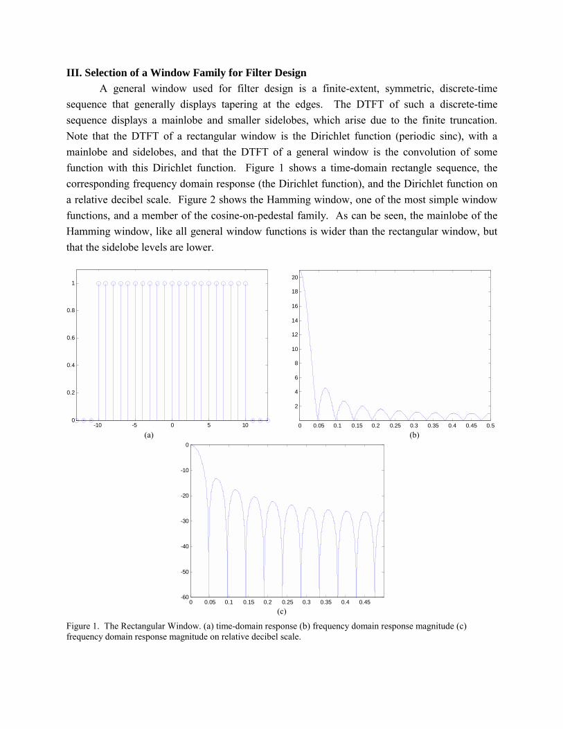
Figure 6. Discrete Prolate Spheroidal Window with N = 101 and W = 0.1. (a) Time-domain response (b) frequency domain response magnitude on relative decibel scale.
-15 -10 -5 0 5 10 150
0.1
0.2
0.3
0.4
0.5
0.6
0.7
0.8
0.9
1
0 0.05 0.1 0.15 0.2 0.25 0.3 0.35 0.4 0.45 0.5-140
-120
-100
-80
-60
-40
-20
0
(a) (b)
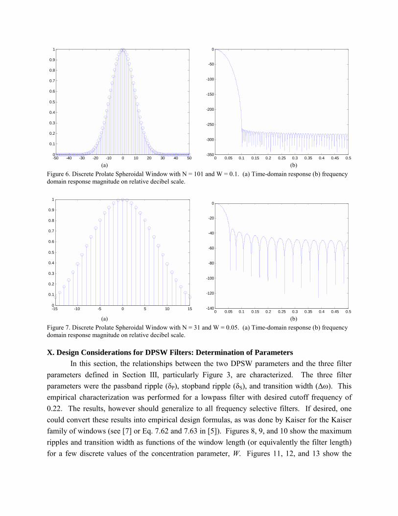
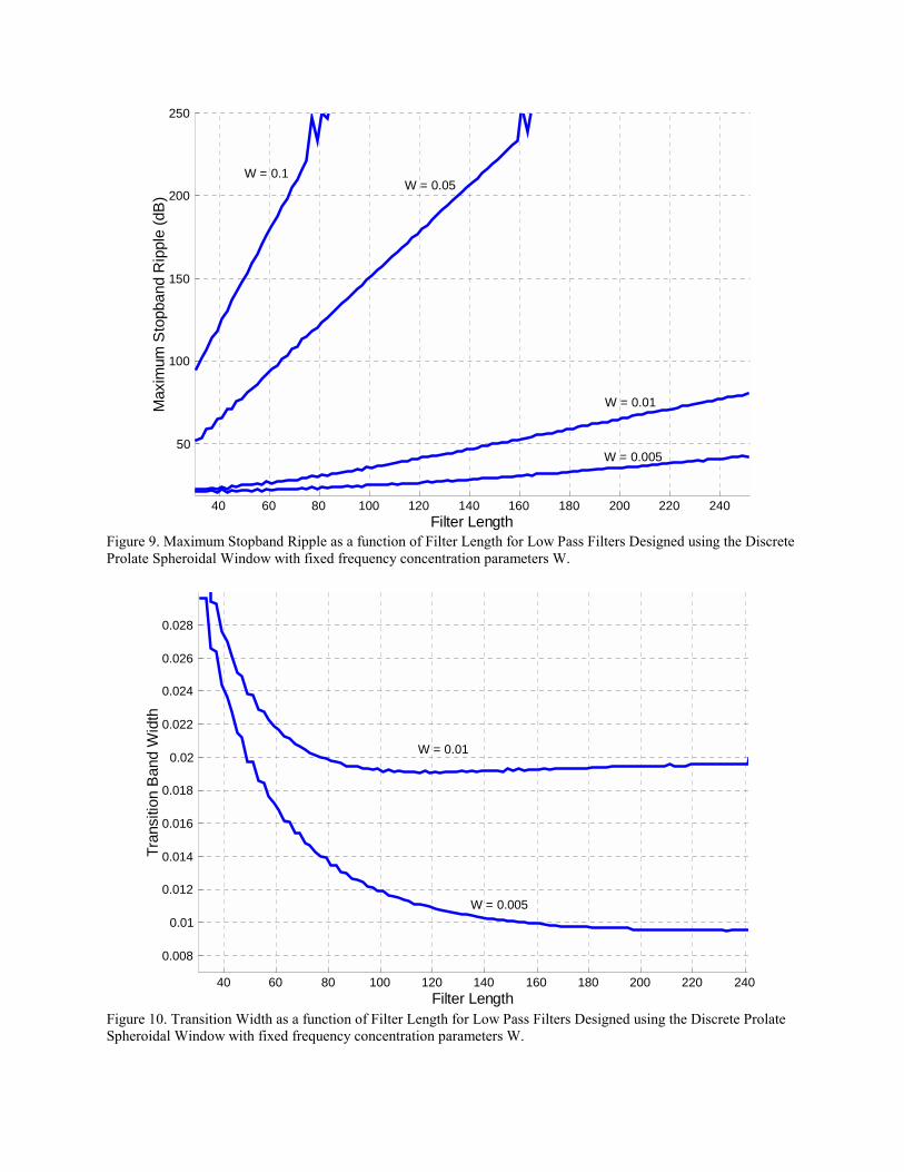
Figure 7. Discrete Prolate Spheroidal Window with N = 31 and W = 0.05. (a) Time-domain response (b) frequency domain response magnitude on relative decibel scale. X. Design Considerations for DPSW Filters: Determination of Parameters In this section, the relationships between the two DPSW parameters and the three filter parameters defined in Section III, particularly Figure 3, are characterized. The three filter parameters were the passband ripple (δP), stopband ripple (δS), and transition width (∆ω). This empirical characterization was performed for a lowpass filter with desired cutoff frequency of 0.22. The results, however should generalize to all frequency selective filters. If desired, one could convert these results into empirical design formulas, as was done by Kaiser for the Kaiser family of windows (see [7] or Eq. 7.62 and 7.63 in [5]). Figures 8, 9, and 10 show the maximum ripples and transition width as functions of the window length (or equivalently the filter length) for a few discrete values of the concentration parameter, W. Figures 11, 12, and 13 show the

maximum ripples and transition width as functions of the concentration parameter for a few discrete values of window length. Following Kaiser, the ripple values are presented in decibels, using the definition
( )δlog20 10−=A (11)
Some points to note in these figures include the fact that passband ripple is always slightly greater than stopband ripple, the fact that ripple decreases as filter length increases and as the concentration parameter W increases. Furthermore, the transition width is almost exactly a linear function of W, in fact given by 2W, and is nearly independent of the filter length (Figure 10 demonstrates the slight dependence).
Appendix 2 gives a listing of MATLAB code that may be used to calculate the three filter parameters of a given filter.
40 60 80 100 120 140 160 180 200 220 240
50
100
150
200
250
Filter Length
Max
imum
Pas
sban
d R
ippl
e (d
B)
W = 0.005
W = 0.001
W = 0.01
W = 0.05
W = 0.1
Figure 8. Maximum Passband Ripple as a function of Filter Length for Low Pass Filters Designed using the Discrete Prolate Spheroidal Window with fixed frequency concentration parameter W.
40 60 80 100 120 140 160 180 200 220 240
50
100
150
200
250
Filter Length
Max
imum
Sto
pban
d R
ippl
e (d
B)
W = 0.005
W = 0.01
W = 0.05 W = 0.1
Figure 9. Maximum Stopband Ripple as a function of Filter Length for Low Pass Filters Designed using the Discrete Prolate Spheroidal Window with fixed frequency concentration parameters W.
40 60 80 100 120 140 160 180 200 220 240
0.008
0.01
0.012
0.014
0.016
0.018
0.02
0.022
0.024
0.026
0.028
Filter Length
Tran
sitio
n B
and
Wid
th
W = 0.005
W = 0.01
Figure 10. Transition Width as a function of Filter Length for Low Pass Filters Designed using the Discrete Prolate Spheroidal Window with fixed frequency concentration parameters W.

0 0.02 0.04 0.06 0.08 0.1 0.12 0.14 0.16 0.18 0.2
50
100
150
200
250
Bandwidth Concentration Parameter W
Max
imum
Pas
sban
d R
ippl
e
N = 31
N = 51
N = 71
N = 101
N = 201
Figure 11. Maximum Passband Ripple as a function of frequency concentration parameter W for Low Pass Filters Designed using the Discrete Prolate Spheroidal Window with fixed Filter Length.
0 0.02 0.04 0.06 0.08 0.1 0.12 0.14 0.16 0.18 0.2
50
100
150
200
250
Bandwidth Concentration Parameter W
Max
imum
Sto
pban
d R
ippl
e
N = 31
N = 51
N = 71
N = 101
N = 201
Figure 12. Maximum Stopband Ripple as a function of frequency concentration parameter W for Low Pass Filters Designed using the Discrete Prolate Spheroidal Window with fixed Filter Length.

0 0.05 0.1 0.15 0.2 0.25
0
0.05
0.1
0.15
0.2
0.25
0.3
0.35
0.4
0.45
0.5
Bandwidth Concentration Parameter W
Tran
sitio
n Ba
nd W
idth
N = 31 N = 51 N = 71 N = 101 N = 201
Figure 13. Transition Width as a function of frequency concentration parameter W for Low Pass Filters Designed using the Discrete Prolate Spheroidal Window with fixed Filter Length. The function appears noisy due to numerical problems. XI. Comparison of DPSW-Filters and other Filters In this penultimate section, a comparison of filters designed using the discrete prolate spheroidal window and filters designed using other methods is made. The two error criterion that were first considered in Sections I and II will be used to make this comparison, namely integrated squared error and Chebyshev error. Design methods compared to DPSW include the constrained least squares method of Selesnick, Lang, and Burrus, the Parks-McClellan optimal Chebyshev method, and the use of other window functions. The Kaiser family, the Hanning window, the Hamming window, and the rectangular window are considered.
Note that the integration performed in calculating the integrated squared error is performed over the entire frequency axis from 0 to 0.5, but the maximization performed in calculating the Chebyshev error is only performed over the passband as delineated from 0 to the left edge of the transition width, marked in Figure 3. Numerical integration with a composite 4-point Newton-Cotes quadrature rule was used [19]. Box B gives an overview of numerical integration with the Newton-Cotes rule. Appendix 3 lists MATLAB code that may be used to calculate the integrated squared error and the Chebyshev error (a simplification of code from Appendix 2), and a utility function.

A
howeveof lengtChebysh15 showand FigtransitioA comwindow
Box B: Numerical Integration [19] An m-point quadrature rule Q for the definite integral
( )∫=b
a
dfI ωω (B.1)
is an approximation of the form
( ) ( )∑=
−=m
kkk fwabQ
1ω (B.2)
The abscissas, ωk, and the weights, wk, define the quadrature rule and are chosen so Q ≈ I. A composite quadrature rule may be formed by applying the quadrature rule to portioned subintervals of the interval between the limits of integration. The Newton-Cotes family of quadrature rules are derived by integrating uniformly spaced polynomial interpolants of the integrand f(ω), and include the trapezoidal rule and Simpson rule as low order cases. The weights in Equation (B.2) for the lowest ordered Newton-Cotes rules are given in Table B-1.
Order (m) Weights (wk) 2 (Trapezoidal) [ ]2
121
3 (Simpson) [ ]61
64
61
4 [ ]81
83
83
81
5 [ ]907
9032
9012
9032
907
6 [ ]28819
28875
28850
28850
28875
28819
Table B-1. Weights for Newton-Cotes Quadrature Rules
s in Section X, for all methods, a lowpass filter with desired cutoff of 0.22 is designed, r generalization to all frequency selective filters should be possible. In all cases, a filter h 51 is considered. Figure 14 shows the integrated squared error as a function of ev error for the constrained least squares filter design method, which is optimal. Figure s the same function for filters designed with DPSW, and similarly Figure 16 for Kaiser, ure 17 for Parks-McClellan. Since the Parks-McClellan algorithm requires a finite n region, it was specified symmetrically around the desired cutoff frequency and varied. parison of these four methods, along with Hamming, Hanning, and Rectangular ing is given in Figure 18.

0 0.01 0.02 0.03 0.04 0.05 0.06 0.07 0.08 0.09 0.12
2.5
3
3.5
4
4.5
5x 10
-3
Chebyshev error δ
Inte
grat
ed S
quar
ed E
rror |
|E||2
Figure 14. Tradeoff Curve between Chebyshev Error and Integrated Squared Error for Lowpass Filters designed using the Constrained Least Squares Method.
0 0.01 0.02 0.03 0.04 0.05 0.06 0.07 0.08 0.09 0.12
2.5
3
3.5
4
4.5
5x 10⁻³
Chebyshev error δ
Inte
grat
ed S
quar
ed E
rror |
|E||2
Figure 15. Tradeoff Curve between Chebyshev Error and Integrated Squared Error for Lowpass Filters designed using the Discrete Prolate Spheroidal Window Method.

0 0.01 0.02 0.03 0.04 0.05 0.06 0.07 0.08 0.09 0.12
2.5
3
3.5
4
4.5
5x 10⁻³
Chebyshev error δ
Inte
grat
ed S
quar
ed E
rror |
|E||2
Figure 16. Tradeoff Curve between Chebyshev Error and Integrated Squared Error for Lowpass Filters designed using the Kaiser Window Method.
0 0.01 0.02 0.03 0.04 0.05 0.06 0.07 0.08 0.09 0.12
2.5
3
3.5
4
4.5
5x 10⁻³
Chebyshev error δ
Inte
grat
ed S
quar
ed E
rror |
|E||2
Figure 17. Tradeoff Curve between Chebyshev Error and Integrated Squared Error for Lowpass Filters designed using the Parks-McClellan Method.

0 0.01 0.02 0.03 0.04 0.05 0.06 0.07 0.08 0.09 0.12
2.5
3
3.5
4
4.5
5x 10⁻³
Chebyshev error δ
Inte
grat
ed S
quar
ed E
rror |
|E||2
CLSDPSWKaiserRemezRectHammingHanning
Figure 17. Comparison of Tradeoff Curves between Chebyshev Error and Integrated Squared Error for Lowpass Filters designed using Constrained Least Squares (CLS), Discrete Prolate Spheroidal Window (DPSW), Kaiser Window (Kaiser), Parks-McClellan Algorithm (Remez), Rectangular Window (Rect), Hamming Window (Hamming), and Hanning Window (Hanning).
It is evident from Figure 17 that the optimal constrained least squares method produces the best results, that the Parks-McClellan algorithm is able to match constrained least squares for some portions of the tradeoff curve, and that the discrete prolate spheroidal window is the best among the window functions. It is interesting to note that although the Kaiser window is designed as an approximation to the DPSW, it has slightly worse performance. Furthermore, the Hamming and Hanning windows are clearly suboptimal.
A listing of MATLAB code for generating various filters with different methods is given in Appendix 4.
XII. On the Use of Discrete Prolate Spheroidal Windows for Spectral Analysis Although the discrete prolate spheroidal window was found to be suboptimal for filter design in the integrated squared error-Chebyshev error tradeoff, it was found to be the best window for this application among those compared. This result suggests that the discrete prolate spheroidal window may find use as a good window for spectral analysis. Windowing is in fact,

more central to spectral analysis than to filter design, which allows greater use of optimization theory. The slightly better performance of the DPSW over the Kaiser window suggests that this benefit would carry over into spectral analysis and since the Kaiser window is widely used for spectral analysis, the DPSW may provide performance gains in that field. In order to facilitate the use of discrete prolate spheroidal windows for spectral analysis, Verma, Bilbao, and Meng have determined empirical formulas relating the window length and the bandwidth concentration factor W to relative peak sidelobe height [20], similar to the empirical formulas determined for Kaiser windows [21].
References [1] E.A. Guillemin, “What is Nature’s Error Criterion?,” IRE Trans. Circuit Theory, vol. 1, no.1, pp. 76, Mar. 1954.
[2] E.A. Guillemin, “What is Nature’s Error Criterion?,” IRE Trans. Circuit Theory, vol. 1, no. 1, pp. 70-71, Sep. 1954.
[3] B. Hutchins, Basic Elements of Digital Signal Processing [Online]. Available: http://courses.ece.cornell.edu/ece426/files/filtc12.pdf.
[4] I.W. Selesnick, M. Lang, and C.S. Burrus, “Constrained Least Square Design of FIR Filters without Specified Transition Bands,” IEEE Trans. Signal Processing, vol. 44, no. 8, pp. 1879-1892, Aug. 1996.
[5] A.V. Oppenheim and R.W. Schafer, Discrete-Time Signal Processing, Upper Saddle River, New Jersey: Prentice Hall, 1999, pp. 465-485.
[6] F.J. Harris, “One the Use of Windows for Harmonic Analysis with the Discrete Fourier Transform,” Proc. IEEE, vol. 66, no. 1, pp. 51-83, Jan. 1978.
[7] J.F. Kaiser, “Nonrecursive Digital Filter Design using the I0-sinh Window Function,” in Proc. 1974 IEEE International Symposium on Circuits and Systems, April 22-25, 1974, San Francisco, CA, pp. 20-23.
[8] D. Slepian and H.O. Pollak, “Prolate Spheroidal Wave Functions, Fourier Analysis, and Uncertainty—I,” Bell System Technical Journal, vol. 40, pp. 43-64, 1961.
[9] H.J. Landau and H.O. Pollak, “Prolate Spheroidal Wave Functions, Fourier Analysis, and Uncertainty—II,” Bell System Technical Journal, vol. 40, pp. 65-84, 1961.
[10] H.J. Landau and H.O. Pollak, “Prolate Spheroidal Wave Functions, Fourier Analysis, and Uncertainty—III,” Bell System Technical Journal, vol. 41, pp. 1295-1336, 1962.
[11] D. Slepian, “Prolate Spheroidal Wave Functions, Fourier Analysis, and Uncertainty—IV: Extensions to Many Dimensions; Generalized Prolate Spheroidal Functions,” Bell System Technical Journal, vol. 43, pp. 3009-3058, 1964.
[12] D. Slepian, “Some Comments on Fourier Analysis, Uncertainty and Modeling,” SIAM Review, vol. 25, no. 3, pp. 379-393, Jul. 1983.
[13] D.W. Tufts, and J.T Tufts, “Designing Digital Low-Pass Filters—Comparison of Some Methods and Criteria,” IEEE Trans. Audio and Electroacoustics, vol. AU-18, no. 4, pp. 487-494, Dec. 1970.
[14] A. Papoulis and M.S. Bertran, “Digital Filtering and Prolate Functions,” IEEE Trans. Circuit Theory, vol. CT-19, no. 6, pp. 674-681, Nov. 1972.
[15] A. Eberhard, “An Optimal Discrete Window for the Calculation of Power Spectra,” IEEE Trans. Audio and Electroacoustics, vol. AU-21, no. 1, pp. 37-43, Feb. 1973.
[16] D. Slepian, “Prolate Spheroidal Wave Functions, Fourier Analysis, and Uncertainty—V: The Discrete Case,” Bell System Technical Journal, vol. 57, no. 5, pp. 1371-1430, May-Jun. 1978.
[17] F.A. Grunbaum, “Toeplitz Matrices Commuting with Tridiagonal Matrices,” Linear Algebra and Its Applications, vol. 40, pp. 25-36, 1981.
[18] B.N. Beresford, The Symmetric Eigenvalue Problem, Philadelphia: Society fo Industrial and Applied Mathematics, 1998.
[19] C.F. Van Loan, Introduction to Scientific Computing, Upper Saddle River, New Jersey: Prentice Hall, 2000, pp. 136-148.
[20] T. Verma, S. Bilbao, and T.H.Y. Meng, “The Digital Prolate Spheroidal Window,” in Proc. IEEE Int. Conf. Acoustics, Speech, and Signal Processing, pp. 1351-1354, May 7-10, 1996.
[21] J.F. Kaiser and R.W. Schafer, “On the Use of the I0-Sinh Window for Spectrum Analysis,” IEEE Trans. Acoustics, Speech, and Signal Processing, vol. ASSP-28, no. 1, pp. 105-107, Feb. 1980.

Appendix 1 – MATLAB Code for Computing Discrete Prolate Spheroidal Windows
function X = prolate(N,W)%PROLATE Digital Prolate Spheroidal Window.% PROLATE(N,W) returns the W-valued N-point Digital Prolate Spheroidal Window.%% See also KAISER, BARTLETT, BLACKMAN, BOXCAR, CHEBWIN, HAMMING, HANN,% and TRIANG.
% Lav Varshney, Cornell University, ECE 426% February 6, 2004
even = 0;if(mod(N,2) == 0)
N = 2*N + 1;even = 1;
end
%set up the tridiagonal T matrixT = diag(((((N-1)/2)-(1:N)+1).^2)*cos(2*pi*W)) + ...
diag(0.5.*((2:N)-1).*(N-(2:N)+1),1) + diag(0.5.*((2:N)-1).*(N-(2:N)+1),-1);
%compute the eigenvector associated with the dominant eigenvalueX = eigpower(T);
if(even)X = X(2:2:end);
end
function [x,lambda] = eigpower(A,tol,x)%EIGPOWER Calculate dominant eigenvalue, corresponding eigenvector using power method% [V,L] = EIGPOWER(A,T,X) calculates the dominant eigenvalue, L, and corresponding% eigenvector, V, of the matrix A. T is an argument that specifies the tolerance% for convergence of the eigenvalue computed. X is an argument that represents an% initial guess for the eigenvector. The maximum element of X must be 1.%% [V,L] = EIGPOWER(A,T) uses a default starting guess of [1 zeros(1,length(A)-1)]'%% [V,L] = EIGPOWER(A) uses same default starting guess, and a tolerance of 10^-16%% See also EIG, EIGS.
% Lav Varshney, Cornell University, ECE 426% February 6, 2004
%make sure matrix is square[m,n] = size(A);if (m ~= n)
error('Matrix must be square.');end
if (nargin == 3)if(length(x) ~= m)
error('Initial guess must be same size as matrix.');endif(max(abs(x)) ~= 1)
error('Initial guess must have largest entry 1 (in magnitude).');end
elsex = [1 zeros(1,m-1)]';
end

%set default toleranceif (nargin == 1)
tol = 1e-16;end
%maximum number of iterationsmaxiter = 100000;
%stopping criterion, change in eigenvalue between iterationsdif = Inf;lambda_old = Inf;
%make the matrix sparse, to quicken arithmetic operationsA = sparse(A);
ii = 0;while((ii < maxiter) & (dif > tol))
y = A*x;[t r] = max(abs(y));
%estimate for eigenvaluelambda = y(r);
%estimate for eigenvectorx = y/y(r);
dif = abs(lambda_old - lambda);lambda_old = lambda;
ii = ii+1;end
Appendix 2 – MATLAB Code for Calculating Error Parameters for Filters
function [delP,delS,wid] = err(h)%ERR Determines the error criteria values for the filter.% [DP,DS,W] = ERR(h) calculates the maximum passband ripple, DP,% the maximum stopband ripple, DS, and the transition width, W. The ripple% values are in dB. The input parameter is the FIR unit pulse response% of the filter in question, h.
% Lav Varshney, Cornell University, ECE 426% February 21, 2004
%calculate the frequency response of the filter[H,W] = freqz(h,1,10000,1);
%%%%%%calculate the maximum value of frequency magnitude to determine passband ripple[delp,delP_ii] = max(abs(H));
%subtract ideal to get ripple value (assume ideal has magnitude 1)delp = delp - 1;
%convert to dBdelP = 20*log10(delp);
%%%%%%calculate the frequency at which the first zero crossing takes place% this is accomplished by taking advantage of linear phase with pi phase% shifts at zero crossings, so the minimum of the unwrapped angle is the% first zero crossing[m,min_ph_ii] = min(unwrap(angle(H)));
%only consider portion of frequency response after first zero crossingHs = H(min_ph_ii:end);
%stopband ripple is the maximum value in this region (assume ideal has 0 magnitude).[delS,delS_ii] = max(20*log10(abs(Hs)));dels = 10^(delS/20);
%%%%%%to calculate transition width, only consider freqeuncies between% maximum passband ripple and first zero crossingHt = H(delP_ii:min_ph_ii);Wt = W(delP_ii:min_ph_ii);
%find the sample that is closest to (1 - delp)[edge_p, edge_p_ii] = min(abs(abs(Ht) - (1-delp)));edge_p_w = Wt(edge_p_ii);
%find the sample that is closest to dels[edge_s, edge_s_ii] = min(abs(abs(Ht) - dels));edge_s_w = Wt(edge_s_ii);
%difference is the transition widthwid = edge_s_w - edge_p_w;
%convert to positive dB.delS = -delS;delP = -delP;

Appendix 3 – MATLAB Code for Calculating Error Criteria for Filters
function Q = ise(H, H_ideal,m)%ISE Integrated Squared Error.% Q = ISE(H,HI,M) calculates the integrated squared error between the% filter frequency response H, and the ideal response HI. An M-point% composite Newton-Cotes quadrature rule is used to approximate this value.% M = 2 corresponds to the trapezoid rule, and M = 3 corresponds to% Simpson's Rule. Only 2 <= M <= 11 are allowed.
% Lav Varshney, Cornell University, ECE 426% February 21, 2004
%absolute squared errorE2 = (abs(abs(H_ideal)-abs(H))).^2;
%starting frequency pointa = 0;%ending frequency pointb = 0.5;
%weights to perform Newton-Cotes rule as inner productw = NCWeights(m);
%estimate of integralQ = 0;
%first subinterval for composite rulefirst = 1;last = m;
%iterate through all subintervalsfor ii = 1:((length(E2)-1)/(m-1))
%apply Newton-Cotes rule on subinterval, and increase estimateQ = Q + (w'*(E2(first:last)));
%update subintervalfirst = last;last = last+m-1;
end
%normalize for number of subintervals and subinterval length (freqeuncy)Q = (b-a)/((length(E2)-1)/(m-1))*Q;
function delp = err2(H)%ERR2 Determines the maximum passband ripple for the filter.% DP = ERR2(H) calculates the maximum passband ripple, DP.% The input parameter is the frequency response% of the filter in question, H.
% Lav Varshney, Cornell University, ECE 426% February 22, 2004
%calculate the maximum value of frequency magnitude to determine passband ripple[delp,delP_ii] = max(abs(H));
%subtract ideal to get ripple value (assume ideal has magnitude 1)delp = delp - 1;

function w = NCWeights(m)%NCWEIGHTS Newton-Cotes Numerical Integration Weight Vector.% NCWEIGHTS(M) Returns the weights for the M-point Newton-Cotes rule.% M is an integer that is between 2 and 11, inclusive
% This function is modified from C.F. Van Loan, Introduction to ScientificComputing.
% Lav Varshney, Cornell University, ECE 426% February 17, 2004
if m == 1w = 1;
elseif m == 2w = [1 1]'/2;
elseif m == 3w = [1 4 1]'/6;
elseif m == 4w = [1 3 3 1]'/8;
elseif m == 5w = [7 32 12 32 7]'/90;
elseif m == 6w = [19 75 50 50 75 19]'/288;
elseif m == 7w = [41 216 27 272 27 216 41]'/840;
elseif m == 8w = [751 3577 1323 2989 2989 1323 3577 751]'/17280;
elseif m == 9w = [989 5888 -928 10496 -4540 10496 -928 5888 989]'/28350;
elseif m == 10w = [2857 15741 1080 19344 5778 5778 19344 1080 15741 2857]'/89600;
elseif m == 11w = [16067 106300 -48525 272400 -260550 427368 -260550 272400 -48525 106300
16067]'/598752;else
w = [];end
Appendix 4 – MATLAB Code for Comparison of Various Filters
%ideal filterW = 0:5e-5:0.49995;Hideal = ones(10000,1);Hideal(find(W>.22)) = 0;
N = 51;
%constrained least squaresdel = logspace(-1,-5,200);jj = 1;for dd = del
h_fircls = fircls(N-1,[0 .44 1],[1 0],[1+dd dd],[1-dd -dd]);H_fircls = abs(freqz(h_fircls,1,10000,1));msse(ii,jj) = ise(H_fircls,Hideal,4);jj = jj+1;
end
%discrete prolate spheroidal windowh = firls(N-1,2*[0 .22 .22 .5],[1 1 0 0]);B = linspace(.001,.25,200);
jj = 1;for dd = B
win = prolate(N,dd).';hwin = h.*win;Hwin = freqz(hwin,1,10000,1);
del(jj) = err2(Hwin);msse(jj) = ise(Hwin,Hideal,4);
jj = jj+1;end
%Kaiser Windowh = firls(N-1,2*[0 .22 .22 .5],[1 1 0 0]);beta = linspace(0,6,200);
jj = 1;for dd = beta
win = kaiser(51,dd).';hwin = h.*win;Hwin = freqz(hwin,1,10000,1);
del(jj) = err2(Hwin);msse(jj) = ise(Hwin,Hideal,4);
jj = jj+1;end
%Parks-McClellant_wid = linspace(eps,.1,200);
jj = 1;for dd = t_wid
hpm = remez(50,2*[0 .22-dd .22+dd .5],[1 1 0 0]);Hpm = freqz(hpm,1,10000,1);
del(jj) = err2(Hpm);msse(jj) = ise(Hpm,Hideal,4);jj = jj+1;
end

%Rectangularh = firls(N-1,2*[0 .22 .22 .5],[1 1 0 0]);[H,W] = freqz(h,1,10000,1);
del = err2(H);msse = ise(H,Hideal,4);
%Hammingh = firls(N-1,2*[0 .22 .22 .5],[1 1 0 0]);win = hamming(51).';hhamm = h.*win;Hhamm = freqz(hhamm,1,10000,1);
del = err2(Hhamm);msse = ise(Hhamm,Hideal,4);
%Hanningh = firls(N-1,2*[0 .22 .22 .5],[1 1 0 0]);win = hanning(51).';hhann = h.*win;Hhann = freqz(hhann,1,10000,1);
del = err2(Hhann);msse = ise(Hhann,Hideal,4);