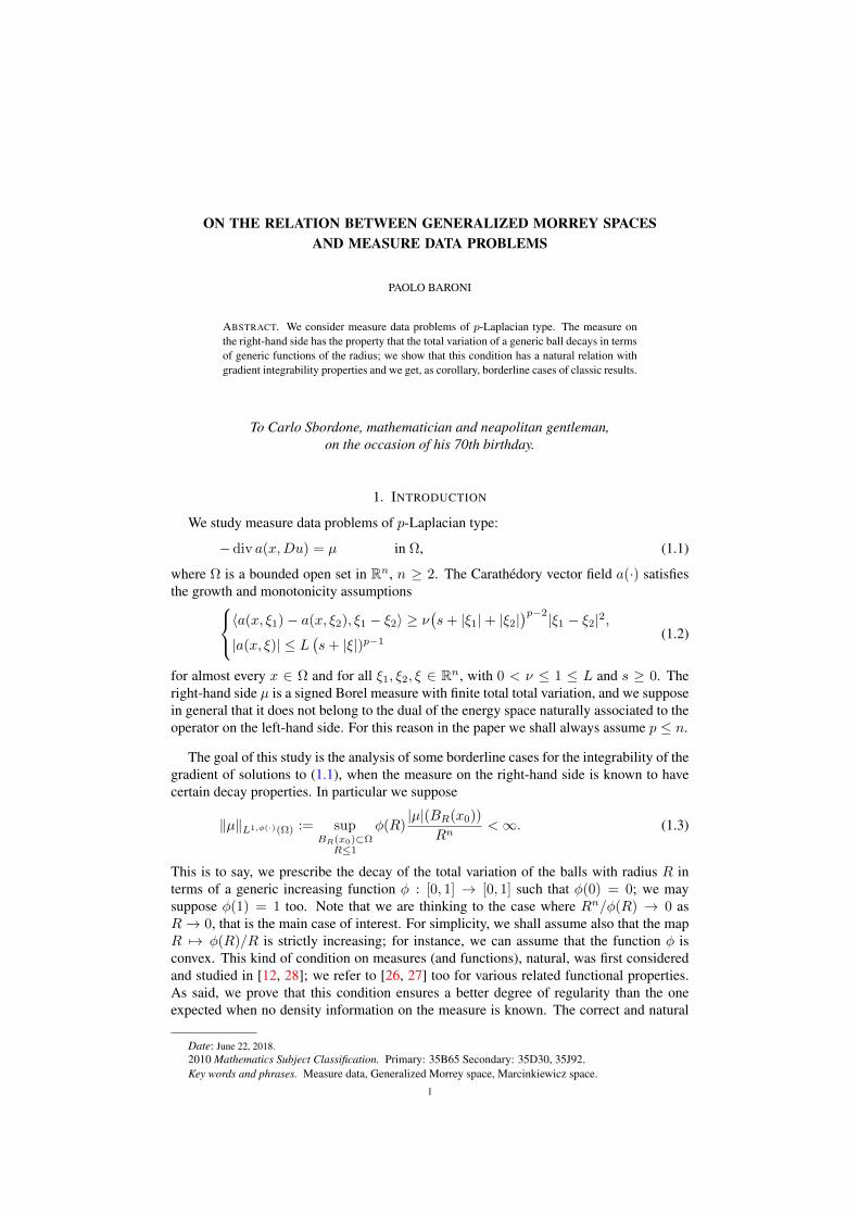
ON THE RELATION BETWEEN GENERALIZED MORREY SPACESAND MEASURE DATA PROBLEMS

PAOLO BARONI

ABSTRACT. We consider measure data problems of p-Laplacian type. The measure onthe right-hand side has the property that the total variation of a generic ball decays in termsof generic functions of the radius; we show that this condition has a natural relation withgradient integrability properties and we get, as corollary, borderline cases of classic results.

To Carlo Sbordone, mathematician and neapolitan gentleman,on the occasion of his 70th birthday.

1. INTRODUCTION

We study measure data problems of p-Laplacian type:

− div a(x,Du) = µ in Ω, (1.1)

where Ω is a bounded open set in Rn, n ≥ 2. The Carathedory vector field a(·) satisfiesthe growth and monotonicity assumptions〈a(x, ξ1)− a(x, ξ2), ξ1 − ξ2〉 ≥ ν

(s+ |ξ1|+ |ξ2|

)p−2|ξ1 − ξ2|2,

|a(x, ξ)| ≤ L(s+ |ξ|)p−1

(1.2)

for almost every x ∈ Ω and for all ξ1, ξ2, ξ ∈ Rn, with 0 < ν ≤ 1 ≤ L and s ≥ 0. Theright-hand side µ is a signed Borel measure with finite total total variation, and we supposein general that it does not belong to the dual of the energy space naturally associated to theoperator on the left-hand side. For this reason in the paper we shall always assume p ≤ n.

The goal of this study is the analysis of some borderline cases for the integrability of thegradient of solutions to (1.1), when the measure on the right-hand side is known to havecertain decay properties. In particular we suppose

‖µ‖L1,φ(·)(Ω) := supBR(x0)⊂Ω

R≤1

φ(R)|µ|(BR(x0))

Rn<∞. (1.3)

This is to say, we prescribe the decay of the total variation of the balls with radius R interms of a generic increasing function φ : [0, 1] → [0, 1] such that φ(0) = 0; we maysuppose φ(1) = 1 too. Note that we are thinking to the case where Rn/φ(R) → 0 asR→ 0, that is the main case of interest. For simplicity, we shall assume also that the mapR 7→ φ(R)/R is strictly increasing; for instance, we can assume that the function φ isconvex. This kind of condition on measures (and functions), natural, was first consideredand studied in [12, 28]; we refer to [26, 27] too for various related functional properties.As said, we prove that this condition ensures a better degree of regularity than the oneexpected when no density information on the measure is known. The correct and natural

Date: June 22, 2018.2010 Mathematics Subject Classification. Primary: 35B65 Secondary: 35D30, 35J92.Key words and phrases. Measure data, Generalized Morrey space, Marcinkiewicz space.

1

2 PAOLO BARONI

way to encode such regularity is in terms of Marcinkiewicz spaces: this is to say, we locallyestimate the decay of the measure of the super level set of Du∣∣x : |Du(x)| > λ

∣∣in terms of functions related to φ. Integrability properties of the gradient of solutions tomeasure data problems are usually formulated in terms of Marcinkiewicz spaces, whichare the optimal ones in view of the behavior of the fundamental solutions; see for instance[2, 10, 20, 22] and [4, 5]. Clearly, generalized Marcinkiewicz spaces must be consideredhere, due to the generality of the situation we are considering.

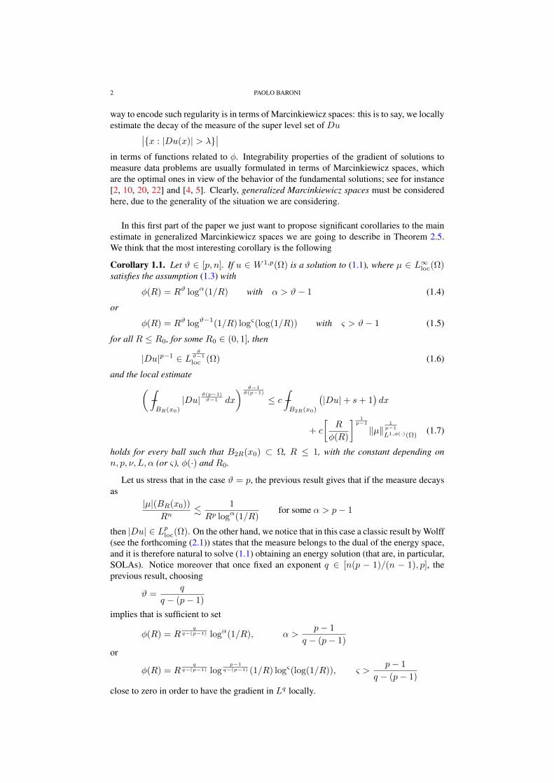
In this first part of the paper we just want to propose significant corollaries to the mainestimate in generalized Marcinkiewicz spaces we are going to describe in Theorem 2.5.We think that the most interesting corollary is the following

Corollary 1.1. Let ϑ ∈ [p, n]. If u ∈ W 1,p(Ω) is a solution to (1.1), where µ ∈ L∞loc(Ω)satisfies the assumption (1.3) with

φ(R) = Rϑ logα(1/R) with α > ϑ− 1 (1.4)

or

φ(R) = Rϑ logϑ−1(1/R) logς(log(1/R)) with ς > ϑ− 1 (1.5)

for all R ≤ R0, for some R0 ∈ (0, 1], then

|Du|p−1 ∈ Lϑϑ−1

loc (Ω) (1.6)

and the local estimate(∫BR(x0)

|Du|ϑ(p−1)ϑ−1 dx

) ϑ−1ϑ(p−1)

≤ c∫B2R(x0)

(|Du|+ s+ 1

)dx

+ c

[R

φ(R)

] 1p−1

‖µ‖1p−1

L1,φ(·)(Ω)(1.7)

holds for every ball such that B2R(x0) ⊂ Ω, R ≤ 1, with the constant depending onn, p, ν, L, α (or ς), φ(·) and R0.

Let us stress that in the case ϑ = p, the previous result gives that if the measure decaysas

|µ|(BR(x0))

Rn.

1

Rp logα(1/R)for some α > p− 1

then |Du| ∈ Lploc(Ω). On the other hand, we notice that in this case a classic result by Wolff(see the forthcoming (2.1)) states that the measure belongs to the dual of the energy space,and it is therefore natural to solve (1.1) obtaining an energy solution (that are, in particular,SOLAs). Notice moreover that once fixed an exponent q ∈ [n(p − 1)/(n − 1), p], theprevious result, choosing

ϑ =q

q − (p− 1)

implies that is sufficient to set

φ(R) = Rq

q−(p−1) logα(1/R), α >p− 1

q − (p− 1)

or

φ(R) = Rq

q−(p−1) logp−1

q−(p−1) (1/R) logς(log(1/R)), ς >p− 1

q − (p− 1)

close to zero in order to have the gradient in Lq locally.

GENERALIZED MORREY SPACES AND MEASURE DATA PROBLEMS 3

One could also consider conditions ensuring Orlicz regularity, in the particular class ofZygmund spaces, for the gradient:

Corollary 1.2. Let ϑ ∈ [p, n) and γ ∈ R or ϑ = n and γ ≥ −1. If u ∈ W 1,p(Ω) is as inCorollary 1.1 and µ ∈ L∞loc(Ω) satisfies the assumption (1.3) with

φ(R) = Rϑ logα(1/R) with α > (γ + 1)(ϑ− 1), (1.8)

or

φ(R) = Rϑ log(γ+1)(ϑ−1)(1/R) logς(log(1/R)) with ς > ϑ− 1, (1.9)

for R ≤ R0 for some R0 ∈ (0, 1]; then

|Du|p−1 ∈ Lϑϑ−1 logγ L (1.10)

locally in Ω and the estimate

‖Du‖L

ϑϑ−1 logγ L(BR(x0))

≤ c∫B2R(x0)

(|Du|+ s+ 1

)dx

+ c

[R

φ(R)

] 1p−1

‖µ‖1p−1

L1,φ(·)(Ω)(1.11)

holds for a constant depending on n, p, ν, L, α (respectively, ς), φ(·) and R0.

We recall the reader that a measurable function g : A ⊂ Rn → R belongs to the Orliczspace L

ϑϑ−1 logγ L(A) = Lϑ

′logγ L(A) for q > 1, γ ∈ R, if∫

A

|g|ϑ′logγ(e+ |g|) dx <∞.

The (averaged) Luxemburg norm employed in (1.11) is defined as follows: for 0 < |A| <∞,

‖ g‖ Lϑ′ logγ L(A) = inf

λ > 0 :

1

λϑ′

∫A

|g|ϑ′logγ

(e+|g|λ

)dx ≤ 1

.

Remark 1.3. Note that the previous results are stated as a priori estimates for energysolutions; it is standard to extend them to SOLAs, that is, solutions of (1.1) obtained asa limit of energy solutions with regularized data; see [3, 8, 15, 18] for details and for theprecise form of the local estimates in this case.

The result contained in Corollary 1.1 is the borderline (in terms of integrability of Du)case of the results in [20, 23] stating the following:

µ ∈ L1,ϑ(Ω), ϑ ∈ [p, n] =⇒ |Du|p−1 ∈Mϑϑ−1

loc (Ω). (1.12)

The space L1,ϑ(Ω) is a classic Morrey space, that in our case corresponds to the simple

choice φ(R) = Rϑ; on the other hand, the spaceMϑϑ−1

loc (Ω) is the localized version of theclassic Marcinkiewicz, or weak Lebesgue, space (see (2.7)-(2.8) for Φ(λ) = λϑ

′). Note

that for ϑ < p the aforementioned classic result of Wolff (see (2.1)) states that L1,ϑ embedsinto the dual space of W 1,p. In the case ϑ = n, the results in [20] give back the classic,sharp result

µ ∈ L1,n(Ω) ≡Mb(Ω) =⇒ |Du| ∈ Mn(p−1)n−1 (Ω),

for which we refer to [11]; notice that the class of measures satisfying (1.3) for ϑ = n isnothing else than the full space of signed Borel measures with finite total total variation.We stress that a different assumption implying the regularity in (1.10), dealing with betterintegrability instead of better decay properties of the datum, is contained in [21, Theorems3 & 12]:

µ ∈ L1,ϑ(Ω) ∩ L logL(Ω) or µ ∈ L logLϑ(Ω)

4 PAOLO BARONI

imply

|Du|p−1 ∈ Lϑϑ−1

loc (Ω);

note that again the improvement should be of “logarithmic type”. We recall the reader thatL logLϑ is the subspace of the Orlicz-Zygmund space L logL made of the functions µsuch that their L logL norm on balls decays in terms of powers of the radius:

‖µ‖L logL(BR) . R−ϑ.

As a final remark in the elliptic setting, we stress that we are able to reproduce anothersubtle phenomenon typical of elliptic equations with measure data: density information onthe measure transfer into density information for the solutions. In particular, a more refinedversion of the result depicted in (1.12), which can still be found in [20, 23], states that notonly Du ∈Mϑ′(BR(x0)) for every ball B2R(x0) ⊂ Ω, but also gives a description of thedecay of this norm in a way perfectly consistent with the decay of the measure. Indeed onehas, for every ball as before

|µ|(BR(x0)) . Rn−ϑ, ϑ ∈ [p, n] =⇒∥∥|Du|p−1

∥∥ϑ′Mϑ′ (BR(x0))

. Rn−ϑ,

see [23, Theorem 4.3]. We refer to the forthcoming Remark 2.7 for a suitable version inour setting.

Result in the setting of classic Morrey spaces are also available in the more difficultparabolic setting: here the condition to be considered involves standard parabolic cylinders

supQR(z0)⊂Ω×(0,T )

|µ|(QR(z0))

RN−ϑ<∞, (1.13)

where QR(z0) = BR(x0)× (t0 −R2, t0 +R2). Note that |QR| = c(n)RN = c(n)Rn+2.The improved integrability of the gradient is again formulated in terms of Marcinkiewicz

spaces: summarizing the results of [7, 4, 5], we have that

µ satisfies (1.13) for some 2 ≤ ϑ ≤ N =⇒ |Du| ∈ Mp−1+ 1ϑ−1

loc

(Ω×(0, T )

),

where u is a solution to the evolutionary analogue of (1.1) under structure of parabolic p-Laplacian type in the style of (1.2). Some results are also available in the case of splittingmeasures, and these are quite surprising in the singular case p < 2 (see [5] for moredetails); global results are also available, at least for p = 2: [6].

Note that many of the results of this paper, if we strengthen our assumptions (in par-ticular, if we impose more regularity on the map x 7→ a(x, ξ)) follow as corollary ofrecent potential estimates, see [16, 17, 18, 19]; in any case many arguments developedhere are necessary to deduce the final form of the estimates, even starting from the point-wise estimates for the gradient. The adaptation of our paper to the parabolic degenerateand singular setting is also not trivial, due mainly to the fact that the lack of scaling of theequation forces to vary the techniques [4, 5] and to obtain results in a different form.

2. NOTATION, THEOREM 2.5 AND TECHNICAL TOOLS

2.1. Notation. This section is devoted to fix the notation we will use in the rest of thepaper. c will denote a generic constant larger than one, possibly varying from line to line.Constants we need to recall will be denoted with special symbols, such as c1, c2, c, C. Rel-evant dependencies will be highlighted between parentheses or after the equations; whennon essential, the dependence on a parameter will be suppressed. We denote by

Br(x0) := x ∈ Rn : |x− x0| < r

GENERALIZED MORREY SPACES AND MEASURE DATA PROBLEMS 5

the open ball with center x0 and radius r > 0; when not important, or clear from thecontext, we shall omit denoting the center as follows: Br ≡ Br(x0). Very often, when nototherwise stated, different balls in the same context will share the same center. We shallalso denoteB1 = B1(0) if not differently specified. Finally, withB being a given ball withradius r and γ being a positive number, we denote by γB the concentric ball with radiusγr. With B ⊂ Rn being a measurable subset with finite and positive measure |B| > 0, andwith g : B → Rk, k ≥ 1, being a measurable map, we shall denote by

(g)B ≡∫Bg(x) dx :=

1

|B|

∫Bg(x) dx

its integral average. We set

p− := minp− 1, 1.

and often we shall denote in short L1,φ(·) for L1,φ(·)(Ω). For σ ∈ R, we shall also usethe notation [log t]σ , when log t is nonnegative, for logσ t. N is the set 1, 2, . . . whileN0 = N ∪ 0.

2.2. Properties of φ. A classic result by Wolff (see [14, Corollary of Theorem 1] and [1]too) implies that the a measure µ belongs to the dual space of W 1,p(Rn) if and only if itsWolff potential Wµ

1,p belongs to L1(Rn, dµ). The local version of this results says that ifthe measure satisfies∫

Ω

∫ 1

0

(µ(Bρ(x))

ρn−p

) 1p−1 dρ

ρdµ(x) = +∞ (2.1)

then it does not belong to the dual of W 1,p(Ω). Since in our case∫Ω

∫ 1

0

(|µ|(Bρ(x))

ρn−p

) 1p−1 dρ

ρd|µ|(x) ≤ ‖µ‖

1p−1

L1,φ(·)(Ω)|µ|(Ω)

∫ 1

0

(ρp

φ(ρ)

) 1p−1 dρ

ρ

once we want to treat the measure data setting, it is natural to suppose that∫ 1

0

(ρp

φ(ρ)

) 1p−1 dρ

ρ=

∫ 1

0

(ρ

φ(ρ)

) 1p−1

dρ = +∞. (2.2)

We shall use the notation

f(ρ) =

(ρ

φ(ρ)

) 1p−1

(2.3)

and we take Ψ : [1,∞)→ (0, 1] as

Ψ(λ) := f−1(λ);

recall that f(1) = 1 and notice that Ψ is decreasing. Our main assumption on Ψ will bethe following one: There exist constants H0 and λ0, both larger than one, and a functionhΨ : [H0,∞)→ [0,∞) such that

Ψ(Hλ) ≥ hΨ(H)Ψ(λ) ∀λ ≥ λ0, H ≥ H0

with limH→+∞

hΨ(H)Hα = +∞ (2.4)

for every α > 1. If a constant will depend on hΨ(·), H0, or on the limit in (2.4), we shallsimply say it depends on φ(·).

For some results, moreover, we will need the following assumption: the existence ofH0, λ0 1 and a function such that φ(Hλ) ≥ hφ(H)φ(λ) for all H ≥ H0, λ ≥ λ0 and,for every β ∈ (0, p),∫ 1

0

[1

sβhφ(1/s)

] nn−1 ds

s<∞. (2.5)

6 PAOLO BARONI

Remark 2.1. We stress that if φ satisfies a∇2 condition of the type

φ(2ρ) ≥ Lφ(ρ) L > 2, for every ρ sufficiently small,

then simple computations show that (2.4) holds for

hΨ(H) = H−log2(L/2)p−1 , H0 =

( L2

) 1p−1

.

In particular, if L = 2p, (2.4) holds with hΨ(H) = 1/H and λ sufficiently large. Clearlyalso (2.5) would hold.

Remark 2.2. Note that when f is not monotone, then, since from (2.2) we have

lim supρ→0

f(ρ) = lim supρ→0

[ρ

φ(ρ)

] 1p−1

= +∞,

we could define Ψ : (1,∞)→ (0, 1) in the following way:

Ψ(λ) := infρ ∈ (0, 1] : f(ρ) < λ for all ρ ∈ [ρ, 1]

.

Ψ is again nonincreasing and such that

limλ→∞

Ψ(λ) = 0, f(Ψ(λ)) = λ, Ψ(f(ρ)) ≥ ρ (2.6)

in their domains. This is sufficient to extend many of our results to the setting where thefunction R 7→ φ(R)/R is not necessarily monotone; we will not focus, however, on thiscase in order not to overload the paper with technical complications.

Before stating the general result we are aiming at, let us introduce the generalizedMarcinkiewicz spaces. For an increasing function Φ such that Φ(0) = 0 and Φ(λ) → ∞as λ→∞ and a measurable set A ⊂ Rn, we define the generalized Marcinkiewicz spacesMΦ(·)(A) as the set of functions such that the following decay condition on level setsholds:

supλ>0

Φ(λ/c)∣∣x ∈ A : |f(x)| > λ

∣∣ <∞ for some c > 0; (2.7)

compare with [9, 10, 24, 25]. Their local variant is defined in the usual way. We set

‖f‖MΦ(·)(A) := infc > 0 : sup

λ>0Φ(λc

)∣∣x ∈ A : |f(x)| > λ∣∣ ≤ 1

(2.8)

and we notice that the quantity, despite the notation we employ, is not a norm since itdoes not, in general, satisfies the triangle’s inequality. Note that is often possible to endowMΦ(·)(A) with a true norm, involving the maximal rearrangement of f , equivalent to‖f‖MΦ(·)(A). It will also be useful to have an averaged, rescaling invariant norms. Wedefine for 0 < |A| <∞

‖f‖MΦ(·)(A) := infc > 0 :

1

|A|supλ>0

Φ(λc

)∣∣x ∈ A : |f(x)| > λ∣∣ ≤ 1

.

(2.9)

Remark 2.3. In the literature the spaces we denote with MΦ(·) are usually called weakgeneralized Marcinkiewicz spaces, or weak Orlicz-Marcinkiewicz spaces in order to dis-tinguish them from so-called Orlicz-Marcinkiewicz spaces, equipped with the norm ex-pressed by the means of the maximal rearrangement mentioned before. In general, thisnorm is just larger than ‖f‖MΦ(·)(Ω) as defined in (2.8); it turns out to be equivalent onlyif Φ grows slowly enough, in the sense that the following condition must hold:∫ t

0

Φ−1(1

s

)ds ≤ C Φ−1

(1

t

)

GENERALIZED MORREY SPACES AND MEASURE DATA PROBLEMS 7

for some constant C and all t > 0. For more details, we refer to [25, Section 7.10] or to[24].

Remark 2.4. Notice that in the classic case of Morrey spaces, where φ(R) = Rϑ, we have

f(ρ) = ρ−ϑ−1p−1 , Ψ(λ) = f−1(λ) = λ−

p−1ϑ−1 ,

λp−1

Ψ(λ)= λ

ϑ(p−1)ϑ−1

and (2.4) is implied by the fact that ϑ ≥ p.

After introducing the generalized Marcinkiewicz spaces, we can state our main result.

Theorem 2.5. Let u ∈ W 1,p(Ω) be a solution to (1.1), where µ ∈ L∞loc(Ω) satisfiesthe assumption (1.3). Assume that R 7→ φ(R)/R is strictly increasing and the technicalassumption (2.4) holds. Then

|Du| ∈ MΦ(·)loc (Ω) with Φ(s) =

sp−1

Ψ(s), s > 0,

and the local estimate

supλ>0

Φ(λ)|x ∈ BR(x0) : |Du(x)| > λ|

|BR(x0)|

≤ Φ

(c

∫B2R(x0)

(|Du|+ s

)dx+ c‖µ‖

1p−1

L1,φ(·)(Ω)

[R

φ(R)

] 1p−1)

(2.10)

holds for every ball B2R(x0) ⊂ Ω and for a constant depending on n, p, ν, L and φ(·).

Note that, in view of Remark 2.4, this result gives back the result described in (1.12)when one considers usual Morrey spaces. For the following two result we shall assumethat (2.4)-(2.5) both hold for every λ > 0, H ≥ 1 with hΨ, hφ defined over [1,∞).

Remark 2.6. An estimate for the Marcinkiewicz norm as defined in (2.8) can be deducedtoo:

‖Du‖MΦ(·)(BR(x0)) ≤ c∫B2R(x0)

(|Du|+ s+ 1

)dx

+ c ‖µ‖1p−1

L1,φ(·)(Ω)

[R

φ(R)

] 1p−1

, (2.11)

where

Φ(s) :=sp−1

cΨ(s)(2.12)

and the constants depend on n, p, ν, L and φ(·).

Observe that in the standard case described in Remark 2.4 it holds

Φ(λ) = λϑ(p−1)ϑ−1 . (2.13)

Remark 2.7. If we assume (2.5) too, we can also describe the decay of the averagedMarcinkiewicz semi-norm:[

φ(R)

R

] 1p−1

‖Du‖MΦ(·)(BR(x0)) ≤ c[|µ|(Ω) + ‖µ‖L1,φ(·)(Ω) + 1

] 1p−1

for a constant depending on n, p, ν, L and φ(·), for R sufficiently small. This is the naturalanalogue of the result encoded in [20, Theorem 1.8] for the standard setting: after somealgebraic manipulations, this result states

Rϑ−1p−1 ‖Du‖

Mϑ(p−1)ϑ−1 (BR(x0))

≤ c[|µ|(Ω) + ‖µ‖L1,φ(·)(Ω)

] 1p−1

.

8 PAOLO BARONI

The averaged norm in the display above is nothing else than, up to universal constants, thestandard averaged Marcinkiewicz norm, that is the norm defined in (2.9) for the choice in(2.13).

2.3. Technical results. We collect here two variants of classic iteration results, both fittingour purposes.

Lemma 2.8. Let R > 0 and f : [R, 2R]→ [0,∞) be bounded and satisfy the relation

f(r1) ≤ 1

2f(r2) + Φ

( A(r2 − r1)γ

)+ B (2.14)

for all R ≤ r1 < r2 ≤ 2R and for constants A,B ≥ 1 and γ > 0. Then there exists aconstant c depending on p, γ and φ(·) such that

f(R) ≤ c[Φ( ARγ

)+ B

].

Proof. We consider, as in [13, Lemma 6.1] the sequence of points Rk with R0 = R and

Rk+1 −Rk = λ(1− λ)kR,

λ ∈ (0, 1) to be chosen. Iterating k times the relation in (2.14), k ∈ N, we get

f(R) = f(R0) ≤ 1

2kf(Rk) +

k−1∑i=0

1

2iG

(A

[λ(1− λ)iR]γ

)+ B

k−1∑i=0

1

2i

and letting k → ∞ we conclude, since for i sufficiently large we have, using (2.4) forβ = 2

Φ

(A

[λ(1− λ)iR]γ

)=

(A

[λ(1− λ)iR]γ

)p−1[Ψ

(A

[λ(1− λ)iR]γ

)]−1

≤(

A[λ(1− λ)iR]

γ

)p−1[Ψ( ARγ

)hΨ

(1

[λ(1− λ)i]γ

)]−1

≤(

A[λ(1− λ)iR]

γ

)p−1[Ψ( ARγ

)(λ(1− λ)i

)2γ]−1

=1

λγ(p+1)

( ARγ

)p−1[Ψ( ARγ

)]−1 1

(1− λ)γ(p+1)i.

The proof is concluded, since a choice of λ such that 2(1 − λ)γ(p+1) > 1 implies theconvergence of the series

∞∑i=0

1

2iG

(A

[λi(1− λ)R]γ

).

Lemma 2.9. Let f, g : [0, 2R]→ R be positive, non-decreasing functions such that

f(ρ) ≤ c0[εf(2r) +

(ρr

)γf(r)

]+ g(r) for all 0 < ρ ≤ r ≤ R, (2.15)

being c0 ≥ 1, ε > 0 and γ > 0. Suppose that there exist H0 ≥ 1 and a (non-decreasing)function h : [H0,∞)→ [1,∞) such that

g(Hs) ≤ h(H)g(s) ∀s > 0,∀H ≥ H0 with∫ 1

0

sσh(1/s)ds

s<∞ (2.16)

for some 0 < σ < γ. Then there exists a constant ε0, depending on γ, σ, c0 and a constantc1, depending only on c0, γ, σ, h(·) such that if ε ≤ ε0, it holds that

f(r1) ≤ c1[(r1

r2

)σf(r2) + g(r1)

]for all 0 < r1 ≤ r2 ≤ 2R. (2.17)

GENERALIZED MORREY SPACES AND MEASURE DATA PROBLEMS 9

Proof. We define τ ≡ τ(γ, σ, c0) < 1/2 as

τ =1

(2γ+1c0)1/(γ−σ)⇐⇒ 2γc0τ

γ−σ ≤ 1

2;

moreover we set ε0 ≡ ε0(γ, σ, c0) = τσ/[2c0] and we take r2 ≤ 2R. Using (2.15) withρ = τ `+1r2 and 2r = τ `r2, ` ∈ N0 and assuming ε ≤ ε0, we get

f(τ `+1r2) ≤ c0[ε0 + 2γτστγ−σ

]f(τ `r2) + g(τ `r2) = τσf(τ `r2) + g(τ `r2);

iterating k times, k ∈ N, we then infer

f(τkr2) ≤ τkσf(r2) +

k−1∑i=0

τ iσg(τk−1−ir2). (2.18)

We split

k−1∑i=0

τ iσg(τk−1−ir2) =

i0−1∑i=0

(. . . ) +k−1∑i=i0

(. . . )

where i0 ≡ i0(γ, σ, c0, H0) is the smallest integer such that τ−i0−2 ≥ H0; clearly we shallonly consider k > i0. For the first sum we simply have

i0−1∑i=0

τ iσg(τk−1−ir2) ≤i0−1∑i=0

g(τk+1r2

τ i0+2

)≤ i0 h(τ−i0−2)g(τk+1r2) = c g(τk+1r2)

with c ≡ c(γ, σ, c0, h(·)). For the second sum, since g is increasing, using (2.16), weestimate

k−1∑i=i0

τ iσg(τk−1−ir2) = − 1

log τ

k−1∑i=i0

τ iσg(τk−1−ir2)

∫ τ i+2

τ i+3

dρ

ρ

≤ c(τ, γ, σ) g(τk+1r2)

k−1∑i=i0

h(1/τ i+2)τ (i+3)σ

∫ τ i+2

τ i+3

dρ

ρ

≤ c g(τk+1r2)

k−1∑i=i0

∫ τ i+2

τ i+3

ρσh(1/ρ)dρ

ρ

≤ c g(τk+1r2)

∫ 1

0

ρσh(1/ρ)dρ

ρ,

with c ≡ c(γ, σ, c0); the last integral is finite thanks to (2.16). Thus, merging the twoestimates into (2.19), we obtain

f(τkr2) ≤ τkσf(r2) + c(γ, σ, c0, h(·))g(τk+1r2) (2.19)

for k > i0 and now the conclusion of the proof is standard. In particular for % ≤ τ i0+1r2

we take k ≥ i0 + 1 such that τk+1r2 < % ≤ τkr2 and we have

f(r1) < f(τkr2) ≤ 1

τσ

(r1

r2

)σf(r2) + c g(r1) ≤ c1

[(r1

r2

)σf(r2) + g(r1)

].

If ρ ∈ (τ i0+1r2, r2], on the other hand, the estimate above is trivial if we further enlargethe constant c1 by a factor depending on σ, τ, i0.

10 PAOLO BARONI

3. MISCELLANEA OF CLASSIC RESULTS

We collect in this section several results already present in the literature. For this, for agiven ball BR(x0) ⊂ Ω, we consider the so-called a(·)-harmonic lifting

div a(x,Dv) = 0 in BR(x0),

v = u on ∂BR(x0);(3.1)

existence follows from standard monotonicity methods, since the boundary datum belongsto W 1,p(BR). The first result we need is a simple comparison estimate.

Lemma 3.1 (Comparison estimate). Let v ∈ u + W 1,p0 (BR(x0)) be the solution to (3.1).

Then for every

q ∈[1,min

n(p− 1)

n− 1, p)

, (3.2)

there exists a constant c ≡ c(n, p, ν, q) such that∫BR(x0)

|Du−Dv|q dx ≤ c[|µ|(B2R(x0))

Rn−1

] qp−1

+ c χp<2

(∫B2R(x0)

(|Du|+ s) dx)q(2−p)[ |µ|(B2R(x0))

Rn−1

]q. (3.3)

Proof. For the comparison estimate∫BR(x0)

|Du−Dv|q dx ≤ c[|µ|(BR(x0))

Rn−1

] qp−1

+ c χp<2

(∫BR(x0)

(|Du|+ s)qdx)2−p

[|µ|(BR(x0))

Rn−1

]q, (3.4)

for q as in (3.2) and c ≡ c(n, p, ν, q), we refer to [20, Lemma 4.1] or [18, Lemma 2] forthe case p ≥ 2 and [23, Lemma 9.2] for the subquadratic case p < 2. In the case p < 2we must use the standard reverse-Holder’s inequality that can be found in [3, Lemma 3.1](see also [5, Proposition 4.3]): with q and c as above, one has∫

BR(x0)

(|Du|+ s)qdx ≤ c

(∫B2R(x0)

(|Du|+s) dx)q

+c

[|µ|(B2R(x0))

Rn−1

] qp−1

.

Since v solves an equation of p-Laplacian type, the following gradient higher integra-bility result holds (see [13, Remark 6.12]):

Proposition 3.2. Let v ∈ u+W 1,p0 (BR(x0)) be the solution of (3.1). Then there exist an

exponent χ ≡ χ(n, p, ν, L) > 1 and a constant c ≡ c(n, p, ν, L) such that∫BR/2(x0)

(|Dv|+ s)pχ dx ≤ c(∫

BR(x0)

(|Dv|+ s) dx

)pχ(3.5)

holds.

Moreover the next Morrey-type estimate encodes the Holder character of solutions to(3.1): see [20] for the result in this form and several applications in the setting of measuredata.

GENERALIZED MORREY SPACES AND MEASURE DATA PROBLEMS 11

Proposition 3.3. Let v ∈ u + W 1,p0 (BR(x0)) be as in Proposition 3.2 and let q ∈ (0, p].

There exist an exponent β0 ≡ β0(n, p, L/ν) ∈ (0, 1] and a constant c ≡ c(n, p, L/ν, q)such that∫

Bρ(x0)

(|Dv|+ s)q dx ≤ c( ρR

)q(β0−1)∫BR(x0)

(|Dv|+ s)q dx

holds for every radius ρ ∈ (0, R].

The previous result, together with our assumption (1.3), allows us to prove a decayestimate that generalize the one available for solutions to measure data equations withMorrey data, see [23, Proposition 10.1].

Lemma 3.4. Let u ∈ C1loc(Ω) be a solution to (1.1) under the assumption (1.3) and (2.5)

on µ ∈ L∞(Ω) and let B2R(x0) ⊂ Ω with R ≤ 1/[2H0]; suppose moreover that R 7→φ(R)/R is monotone increasing. For every exponent q as in (3.2), there exists a constantc depending on n, p, ν, L, q and φ(·) such that∫

BR(x0)

(|Du|+ s)q dx ≤ c[|µ|(Ω) + ‖µ‖L1,φ(Ω)

] qp−1[

R

φ(R)

] qp−1

. (3.6)

Proof. Fix ρ, r ∈ (0, R] with ρ < r and define the p-harmonic lifting v ∈ u+W 1,p0 (Br(x0))

as in (3.1) over Br(x0), being q fixed as in the statement, we have∫Bρ(x0)

(|Du|+ s)q dx ≤ c∫Bρ(x0)

(|Dv|+ s)q dx+ c

∫Bρ(x0)

|Du−Dv|q dx

≤ c(ρr

)q(β0−1)∫Br(x0)

(|Dv|+ s)q dx

+ c( rρ

)n ∫Br(x0)

|Du−Dv|q dx

≤ c(ρr

)q(β0−1)∫Br(x0)

(|Du|+ s)q dx

+ c( rρ

)n ∫Br(x0)

|Du−Dv|q dx.

At this point we estimate, using Lemma 3.1, Young’s inequality only in the case p < 2 and(1.3) ∫

Br(x0)

|Du−Dv|q dx ≤ c[|µ|(B2r(x0))

rn−1

] qp−1

+ c χp<2

(∫B2r(x0)

(|Du|+ s) dx)q(2−p)[ |µ|(B2r(x0))

Rn−1

]q≤ cε

[|µ|(B2r(x0))

Rn−1

] qp−1

+ ε(∫

B2r(x0)

(|Du|+ s) dx)q

≤ cε‖µ‖qp−1

L1,φ

[r

φ(4r)

] qp−1

+ ε(∫

B2r(x0)

(|Du|+ s) dx)q

≤ cε‖µ‖qp−1

L1,φ

[r

φ(r)

] qp−1

+ ε

∫B2r(x0)

(|Du|+ s)q dx;

cε is a constant depending on n, p, ν, L and ε; thus∫Bρ(x0)

(|Du|+ s)q dx ≤ c[(ρr

)n−q(1−β0)∫Br(x0)

(|Du|+ s)q dx

12 PAOLO BARONI

+ ε

∫B2r(x0)

(|Du|+ s)q dx

]+ cε‖µ‖

qp−1

L1,φrn

[r

φ(r)

] qp−1

,

after renaming ε; c depends only on n, p, ν/L.

We can now apply the variant of a classic iteration result in Lemma 2.9 to deduce (3.6):being ε0 the constant appearing in Lemma 2.9 for the choice γ = n − q(1 − β0), σ =n− q(1− β0/2), c0 = c, we take in (2.15) ε = ε0 (and cε = cε0 accordingly) and

f(ρ) =

∫Bρ(x0)

(|Du|+ s)q dx, g(ρ) = cε0‖µ‖qp−1

L1,φρn

[ρ

φ(ρ)

] qp−1

,

we have, using our assumption (2.5), for every H ≥ H0,

g(Hρ) ≤ Hn

[H

hφ(H)

] qp−1

g(ρ)

and, calling β = 1 + (p− 1)(1− β0/2) < p and ε = (p− β)/2, using Holder’s inequality∫ 1

0

sn−q(1−β0/2)(1

s

)n[ 1

shφ(1/s)

] qp−1 ds

s

=

∫ 1

0

[1

sβhφ(1/s)

] qp−1 ds

s=

∫ 1

0

sεqp−1

[1

sβ+p

2 hφ(1/s)

] qp−1 ds

s

≤(∫ 1

0

sεds

s

)1− (n−1)qn(p−1)

(∫ 1

0

[1

sβ+p

2 hφ(1/s)

] nn−1 ds

s

) (n−1)qn(p−1)

for some ε ≡ ε(n, p, q, ν/L) > 0 (note that q/(p− 1) < n/(n− 1)); hence∫ 1

0

sn−q(1−β0/2)(1

s

)n[ 1

shφ(1/s)

] qp−1 ds

s≤ c

(∫ 1

0

[1

sβ+p

2 hφ(1/s)

] nn−1 ds

s

) (n−1)qn(p−1)

≤ c(n, p, q, ν/L, φ(·))

and (2.16) is satisfied. Now we can suppose(ρr

)n−q(1−β0/2)

≤(ρr

)n[ ρ/r

φ(ρ/r)

] qp−1

=(ρr

)nf(ρ/r)

for ρ sufficiently small from (2.4); (2.17) in this situation gives, for all 0 < ρ ≤ r ≤ 2R∫Bρ(x0)

(|Du|+ s)q dx ≤ c[[ ρ/r

φ(ρ/r)

] qp−1

∫Br(x0)

(|Du|+ s)q dx+ ‖µ‖qp−1

L1,φ

[ ρ

φ(ρ)

] qp−1

]≤ c[ ρ

φ(ρ)

] qp−1

[[ 1

rhφ(1/r)

] qp−1

∫Br(x0)

(|Du|+ s)q dx+ ‖µ‖qp−1

L1,φ

]≤ c[ ρ

φ(ρ)

] qp−1

[ ∫Br(x0)

(|Du|+ s)q dx+ ‖µ‖qp−1

L1,φ

]if r ≤ 1/H0. (3.6) follows, since∫

Br(x0)

(|Du|+ s)q dx ≤ c(n, p, ν, q)|µ|(Ω),

see [8, 20].

GENERALIZED MORREY SPACES AND MEASURE DATA PROBLEMS 13

4. THE PROOF OF THEOREM 2.5

We start fixing a ball B2R ≡ B2R(x0) ⊂ Ω, R ≤ 1/2 and arbitrarily an exponent qsuch that

1 < q <n(p− 1)

n− 1< p (4.1)

so that it only depends on n and p: for instance, we can choose the midpoint of the interval[1, n(p− 1)/(n− 1)]. For two intermediate radii R ≤ r1 < r2 ≤ 2R we define

λref =

∫Br2

|Du| dx+M

[|Br2 |

1n|µ|(Br2)

|Br2 |

] 1p−1

+ λ0, (4.2)

with Br2 ≡ Br2(x0), where λ0 appears in (2.4). Moreover we take λ satisfying λ > Bλ0

with B ≥ 1 defined as

B :=

(40r2

r2 − r1

)n(4.3)

In a standard way one can prove that for every λ > Bλref and for almost every point x ofthe super-level set

E(λ,Br1) :=x ∈ Br1(x0) : |Du(x)| > λ

there exists a radius rx < (r2 − r1)/40 such that

λ

40n/p−≤∫Bjrx (x)

|Du| dx+M

[|Bjrx(x)|

1n|µ|(Bjrx(x))

|Bjrx(x)|

] 1p−1

≤ λ (4.4)

for every j ∈ 1, . . . , 40; note that Bjrx(x) ⊂ Br2 . The procedure is nowadays quitestandard, see for instance [4, 5, 20, 23].

We fix now one of these balls Brx(x), rx being the radius defined above, and we notethat one of the following two inequalities must hold:

λ

80n/p−≤∫B2rx (x)

|Du| dx or( λ

80n/p−

)p−1

≤Mp−1 |µ|(B2rx(x))

|B2rx(x)|n−1n

.

(4.5)

The first case. Suppose that the first inequality in (4.5) is in force: for ς ∈ (0, 1) to bechosen, we estimate∫

B2rx (x)

|Du| dx =

∫B2rx (x)∩E(ςλ,Br2 )

|Du| dx+

∫B2rx (x)rE(ςλ,Br2 )

|Du| dx

≤ ςλ∣∣B2rx(x)

∣∣+

∫E(ςλ,B2rx (x))

|Du| dx

≤ ςλ∣∣B2rx(x)

∣∣+∣∣E(ςλ,B2rx(x))

∣∣ 1q′

(∫E(ςλ,B2rx (x))

|Du|q dx) 1q

,

q as in (4.1); enlarging the domain of integration, taking averages and using (4.5)1 yields

λ

80n/p−≤ ςλ+

(|E(ςλ,B2rx(x))||B2rx(x)|

) 1q′(∫

B2rx (x)

|Du|q dx) 1q

. (4.6)

To estimate the last averaged integral in terms of λ, we define the a(·)-comparison liftingv ∈ u+W 1,p

0 (B20rx(x)) as in (3.1) with R = 20rx and x0 = x. Since (4.4) implies both[|µ|(B40rx(x))

(40rx)n−1

] 1p−1

≤ c(n, p)λ

M,

∫B40rx (x)

|Du| dx ≤ λ, (4.7)

14 PAOLO BARONI

a consequence of the comparison estimate (3.4) in this setting is∫B20rx (x)

|Du−Dv|q dx ≤ c[|µ|(B40rx(x))

(40rx)n−1

] qp−1

+ c χp<2

(∫B40rx (x)

(|Du|+ s) dx)(2−p)q

[|µ|(B40rx(x))

(40rx)n−1

]q≤ c λ

q

Mq+ c χp<2

λq

Mq(p−1)≤ c λq

Mp−q, (4.8)

with c depending on n, p and ν. Thus, enlarging the domain of integration several times,using the quasi-subadditivity of the map s 7→ sq and the higher integrability of Proposition3.2 we get∫

B2rx (x)

|Du|q dx ≤ c(q)10n∫B20rx (x)

|Du−Dv|q dx+ c(q)5n∫B10rx (x)

|Dv|q dx

≤ c∫B20rx (x)

|Du−Dv|q dx+ c

(∫B20rx (x)

(|Dv|+ s) dx

)q≤ c

∫B20rx (x)

|Du−Dv|q dx

+c

(∫B20rx (x)

(|Du|+ s) dx+

∫B20rx (x)

|Du−Dv| dx)q

≤ c∫B20rx (x)

|Du−Dv|q dx+ c

(∫B20rx (x)

(|Du|+ s) dx

)qwith c ≡ (n, p, ν, L); at this point, we use (4.8) and (4.7) to get∫

B2rx (x)

|Du|q dx ≤ c λq

for a constant depending on n, p, ν and L; in turn, inserting the last estimate into (4.6) wefinally get

λ

80n/p−≤ ςλ+ c

(|E(ςλ,B2rx(x))||B2rx(x)|

) 1q′

λ

and dividing by λq and absorbing (we fix the value of ς as 160n/p−

)

1

c≤ c

(|E(ςλ,B2rx(x))||B2rx(x)|

) 1q′

.

Summing up, this means that there exists a constant depending on n, p, ν and L such thatif the first alternative in (4.5) holds, then, fixing ς ≡ ς(n, p) as above, we have

|B2rx(x)| ≤ c |E(ςλ,B2rx(x))|.The second case. Suppose instead that the second inequality in (4.5) holds. As a firstconsequence, using (1.3) we have

λp−1 ≤ c(n, p)Mp−1 |µ|(B2rx(x))

|B2rx(x)|n−1n

≤ cMp−1 rnxrn−1x φ(2rx)

= cMp−1 rxφ(rx)

with c ≡ c(n, p) and thus, keeping into account (2.6),

2rx ≤ Ψ( λ

cM

);

hence, as second consequence of (4.5)2

|B2rx(x)| ≤ c(Mλ

)p−1

(2rx)|µ|(B2rx(x)) ≤(cMλ

)p−1

Ψ( λ

cM

)|µ|(B2rx(x))

GENERALIZED MORREY SPACES AND MEASURE DATA PROBLEMS 15

with c ≡ c(n, p). Thus, merging the two alternatives, we have

|B20rx(x)| ≤ c(n)|B2rx(x)|

≤ c |E(ςλ,B2rx(x))|+(cMλ

)p−1

Ψ( λ

cM

)|µ|(B2rx(x)). (4.9)

Covering and iteration. We consider the collection of balls

Eλ := B2rx(x)x∈E(λ,Br1 )

where rx is defined accordingly to (4.4). Using Vitali covering lemma we extract a count-able sub-collection Fλ ⊂ Eλ such that the 5-times enlarged balls cover almost almost allE(λ,Br1) and the balls are pairwise disjoints. This is to say, if we denote the balls of Fλby Bi := B2rxi

(xi), for i ∈ Iλ, being possibly Iλ = N, and with xi ∈ E(λ,Br1), wehave

Bi ∩Bj = ∅ whenever i 6= j and E(λ,Br1) ⊂⋃i∈Iλ

5Bi ∪N , (4.10)

with |N | = 0; remember that since rxi < (r2 − r1)/40 we see that 5Bi = B10rxi(xi) ⊂

Br2 for all i ∈ Iλ. ForH ≥ H0, withH0 appearing in (2.4), to be chosen later we estimate∣∣E(Hλ, r1)∣∣ ≤∑

i∈Iλ

∣∣5Bi ∩ E(2Hλ, r2)∣∣.

We split every term in the following way:∣∣5Bi ∩ E(2Hλ, r2)∣∣ ≤ ∣∣x ∈ 5Bi : |Du(x)|+ s > 2Hλ

∣∣≤∣∣x ∈ 5Bi : |Du(x)−Dvi(x)| > Hλ

∣∣+∣∣x ∈ 5Bi : |Dvi(x)| > Hλ

∣∣ =: Ii + IIi. (4.11)

Here vi is the comparison function solution to (3.1) in 10Bi ≡ B20rzi(xi). We estimate

separately the two pieces: for the first one we use (4.8) and subsequently (4.9) to infer

Ii ≤1

Hλ

∫20Bi

|Du−Dvi| dz ≤c

Hλ· 1

Mp−|20Bi|λ (4.12)

≤ c

HMp−

[|E(ςλ,Bi)|

+(cMλ

)p−1

Ψ( λ

cM

)|µ|(Bi)

].

To estimate the term IIi we use the higher integrability (3.5): for χ > 1 given in Proposi-tion 3.2, we have

IIi ≤( 1

Hλ

)pχ|5Bi|

∫5Bi

(|Dvi|+ s)pχ dz

≤ c

(Hλ)pχ|20Bi|

(∫10Bi

(|Dvi|+ s) dz

)pχ≤ c

Hpχ

[|E(ςλ,Bi)|+

(cMλ

)p−1

Ψ( λ

cM

)|µ|(Bi)

]. (4.13)

Connecting the two estimates (4.12) and (4.13) and plugging the result into (4.11), takinginto account that H ≥ 1, gives∣∣5Bi ∩ E(2Hλ,Qr2)

∣∣ ≤ c [ 1

HMp−+

1

Hpχ

][|E(ςλ,Bi)|

+(cMλ

)p−1

Ψ( λ

cM

)|µ|(Bi)

].

16 PAOLO BARONI

At this point first we choose M ≡M(n, p, ν, L,H) such that HMp− = Hpχ; then, usingthe fact that the Bi are pairwise disjoint, see (4.10), we sum up and we have∣∣E(2Hλ,Br1)

∣∣ ≤ c∗Hpχ|E(ςλ,Br2)|+ c

Ψ(λ)

λp−1|µ|(B2R)

with c∗ depending only on n, p, ν, L but not on H; c depends also on H . Notice that

Ψ( λ

cM

)≤ c(M,φ(·))Ψ(λ)

follows from (2.4). In turn, recalling that ς is a constant depending only on n and p, we canfurther simplify the previous estimate in the following way, renaming λ and H (λ ↔ ςλand H ↔ 2H/ς):∣∣E(Hλ,Br1)

∣∣ ≤ c∗Hpχ|E(λ,Br2)|+ c

Ψ(λ)

λp−1|µ|(B2R)

and this estimate holds for every λ ≥ Bλref , with λref defined in (4.2) and B as in (4.3),and for every H sufficiently large, in particular at this point larger than 2H0/ς . Now wemultiply both sides for the quantity (Hλ)p−1/Ψ(Hλ) and we get

(Hλ)p−1

Ψ(Hλ)

∣∣E(Hλ,Br1)∣∣ ≤ c∗

Hpχ

(Hλ)p−1

Ψ(Hλ)|E(λ,Br2)|+ c

Ψ(λ)

λp−1|µ|(B2R)

≤ c∗Hp(χ−1)+1hΨ(H)

λp−1

Ψ(λ)|E(λ,Br2)|+ c |µ|(B2R).

The local result in (2.10) now follows in a standard way, reabsorbing the appropriate quan-tities on the right-hand side. Indeed, first we take the supremum with respect to λ in[Bλref ,+∞) and then we add to both sides the sup of the same quantity over (0, Bλref).This gives, after using the monotonicity of s 7→ sp−1/Ψ(s) and changing variable in thesupremum in the left-hand side

supλ>0

λp−1

Ψ(λ)

∣∣E(λ,Br1)∣∣ ≤ 1

2supλ>0

λp−1

Ψ(λ)|E(λ,Br2)|

+ c(Bλref)

p−1

Ψ(Bλref)|B2R| + c |µ|(B2R),

since by (2.4) with β = p(χ − 1) + 1 > 1 we can take H ≡ H(n, p, ν, L, φ(·)) so largethat

c∗Hp(χ−1)+1hΨ(H)

≤ 1

2. (4.14)

Since a direct computation, taking into account (1.3), shows that

Bλref ≤c

(r2 − r1)n

[ ∫B2R

(|Du|+ s) dx+Rn[

R

φ(R)

] 1p−1

‖µ‖1p−1

L1,φ(·) + λ0

]=:

λ1

(r2 − r1)n,

with c ≡ c(n, p, ν, L, φ(·)); a standard iteration result (we use the version in Lemma 2.8)implies that we can reabsorb the supremum on the right-hand side and obtain

supλ>0

λp−1

Ψ(λ)

∣∣E(λ,BR)∣∣ ≤ (λ1/R

n)p−1

Ψ(λ1/Rn)|B2R|+ c |µ|(B2R).

Therefore, with

λ ≡ λ(u) := C

∫B2R

(|Du|+ s) dx+ C

[R

φ(R)

] 1p−1

‖µ‖1p−1

L1,φ(·) + Cλ0 (4.15)

GENERALIZED MORREY SPACES AND MEASURE DATA PROBLEMS 17

C ≡ C(n, p, ν, L, φ(·)) sufficiently large, we have

1

|BR|supλ>0

λp−1

Ψ(λ)

∣∣E(λ,BR)∣∣ ≤ λp−1

Ψ(λ)(4.16)

using again the monotonicity of s 7→ sp−1/Ψ(s); we indeed can estimate

|µ|(B2R)

|B2R|≤ c(n)‖µ‖L1,φ(Ω)

2R

φ(2R)≤ λp−1 ≤ λp−1

Ψ(λ)

and this finally proves (2.10). Now, in order to get the estimate in (2.11), we use a rescalingargument: once fixed B2R(x0) ⊂ Ω, if we define

u : B1 → R, u(x) =u(x0 + 2Rx)

2Rf(R)λ

then it is easy so see that u solves

div a(x,Du) = µ in B1

with

a(x, ξ) =a(x, λf(R)ξ)

[λf(R)]p−1, s =

s

λf(R), µ(x) = R

µ(x0 +Rx)

[λf(R)]p−1,

and for Br(y0) ⊂ B2, y0 ∈ B1, r ≤ 1,

|µ|(Br(y0)) =R1−n

[λf(R)]p−1|µ|(BrR(x0 + y0)),

so that

µ ∈ L1,φ(·)(B1) for φ(r) =φ(rR)

φ(R)and ‖µ‖L1,φ(·)(B1) ≤

‖µ‖L1,φ(·)

[λ(u)f(R)]p−1

R

φ(R).

Simple computations show that

f(r) =

[r

φ(r)

] 1p−1

=

[φ(R)r

φ(rR)

] 1p−1

,

Ψ(λ) = f−1(λ) =1

RΨ

([ R

φ(R)

] 1p−1

λ

)=

1

RΨ(f(R)λ

);

we observe that (2.4) holds for Ψ with λ0 replaced by λ0/f(R) but for the same functionhΨ; finally, we also have φ(1) = 1 and Ψ(1) = 1. Therefore, if we want to apply theestimate in (4.16) to u between B1/2 and B1, we compute

λ(u) = C

∫B1

(|Du|+ s) dx+ C

[1

φ(1)

] 1p−1

‖µ‖1p−1

L1,φ(·)(B1)+ C

λ0

f(R)

≤ 1

f(R)

[C

λ(u)

∫B2R(x0)

(|Du|+ s) dx+ C

[R

φ(R)

] 1p−1 ‖µ‖

1p−1

L1,φ(·)

λ(u)+ Cλ0

]≤ 2Cλ0

f(R)

so we get

supλ>0

λp−1

Ψ(λ)

∣∣y ∈ B1/2 : |Du(y)| > λ∣∣ ≤ [λ(u)]p−1

Ψ(λ(u))≤ c λ

p−10

Ψ(λ0)

φ(R)

R·R = cφ(R).

We stress that

c ≥ supλ>0

λp−1

Ψ(λ)φ(R)

∣∣y ∈ B1/2 : |Du(y)| > λ∣∣

18 PAOLO BARONI

= supλ>0

λp−1

Ψ(λ)φ(R)

|x ∈ BR(x0) : |Du(x)| > λ(u)f(R)λ

|

|BR(x0)|

= supλ>0

[λ/f(R)]p−1

Ψ(λ/f(R))φ(R)

|x ∈ BR(x0) : |Du(x)|/λ(u) > λ

|

|BR(x0)|

and then, in view of (2.9) and the explicit expression of the function on the left-hand side

[λ/f(R)]p−1

Ψ(λ/f(R))φ(R)=λp−1

Ψ(λ)· 1

[f(R)]p−1· R

φ(R)=λp−1

Ψ(λ),

this gives

‖Du/λ(u)‖MΦ(·)(BR(x0)) =‖Du‖MΦ(·)(BR(x0))

λ(u)≤ 1

that is (2.11).

5. PROOFS OF COROLLARIES

In order to prove quickly the corollaries, we first give recall some calculus results for aclass of functions having “almost monomial” behavior. We suppose ϕ : [0,∞) → [0,∞)to be C1(0,∞) and to satisfy the condition

1 < g0 ≤ϕ′(s)s

ϕ(s)≤ g1 <∞ for all s > 0. (5.1)

We introduce the notation A ≈ B to denote in short that there exists a constant cϕ ≡c(g0, g1) ≥ 1 such that B/cϕ ≤ A ≤ cϕB. The first property we need, that can bechecked by a simple computation, is that if ϕ satisfies (5.1), then all the functions

ϕ−1(s),1

ϕ(1/s)and [ϕ(s)]` for any ` > 0

satisfy (5.1) for a constant depending on g0, g1 and possibly on ` (notice that (5.1) impliesthat ϕ is increasing thus invertible). Moreover,

d

ds

s

ϕ(s)=ϕ(s)− sϕ′(s)

[ϕ(s)]2≈ − 1

ϕ(s),

d

dsϕ−1(s) ≈ ϕ−1(s)

s. (5.2)

We then note that for q > 1, γ, ς ∈ R the functions

t 7→ tq logγ(e/t), t 7→ tq logγ(1/t), logς log(1/t) (5.3)

satisfy (5.1) for t ∈ (0, R), R ≡ R(γ, ς) ≤ R0 and for constants depending only on q.

5.1. A scaling procedure. We start with a rescaling similar to that used to prove Remark2.6. We set u(x) = u(x0 + x)/λ where λ is the quantity

c

∫B2R(x0)

(|Du|+ s+ 1) dx+ c ‖µ‖1p−1

L1,φ(·)(Ω)

[R

φ(R)

] 1p−1

,

with c the constant appearing in (2.10); u solves

div a(x,Du) = µ in B2R(0), a(x, ξ) =a(x, λξ)

λp−1, µ =

µ

λp−1,

s = s/λ, and is such that

c

∫B2R(0)

(|Du|+ s+ 1) dx+ c ‖µ‖1p−1

L1,φ(·)(Ω)

[R

φ(R)

] 1p−1

=1

λ

[c

∫B2R(x0)

(|Du|+ s) dx+ c ‖µ‖1p−1

L1,φ(·)(Ω)

[R

φ(R)

] 1p−1]

+ c ≤ c.

GENERALIZED MORREY SPACES AND MEASURE DATA PROBLEMS 19

Thus applying (2.10) to u gives

supλ>0

Φ(λ)|x ∈ BR : |Du(x)| > λ|

|BR|≤ c, (5.4)

where c is a universal constant. Once we will get (5.6) and the analogue for Corollary 1.2,it will be easy to scale back to u, obtaining respectively (1.7) and (1.11).

5.2. Proof of Corollary 1.1. We take φ satisfying (5.1) and such that f , as defined in(2.3), is decreasing and smooth. We write, using Fubini’s theorem,∫

BR

|Du|ϑ(p−1)ϑ−1 dx = c(n, p)

∫ ∞0

λϑ(p−1)ϑ−1

|x ∈ BR : |Du(x)| > λ||BR|

dλ

λ

≤ c+ c

∫ ∞f(R)

λϑ(p−1)ϑ−1

|x ∈ BR : |Du(x)| > λ||BR|

dλ

λ

=: c [1 + I];

the constant c depends on n, p,R0, α, or n, p,R0, ς , depending whether we are considering(1.4) or (1.5). To estimate the last term, in both cases we use (5.4), recalling that Ψ = f−1:

I ≤ c∫ ∞f(R)

λϑ(p−1)ϑ−1

f−1(λ)

λp−1

dλ

λ= c

∫ R

0

[f(ρ)]ϑ(p−1)ϑ−1

ρ

[f(ρ)]p−1

dρ

ρ

= c

∫ R

0

[f(ρ)]p−1ϑ−1 dρ

= c

∫ R

0

[ρ

φ(ρ)

] 1ϑ−1

dρ, (5.5)

c depending only on n, p and R0. In the first equality we changed variable ρ = f−1(λ)and we used the following facts:

d

dρ

ρ

φ(ρ)≈ − 1

φ(ρ), f ′(ρ) ≈ −f(ρ)

φ(ρ)

ρ

1

φ(ρ)= −f(ρ)

ρ,

dλ

λ≈ −dρ

ρ,

due to (5.2). Now it is immediate to see that if φ is as in (1.4) or as in (1.5) in (0, R) theintegral on the right-hand side in (5.5) is finite; moreover the functions satisfy (5.1) (see(5.3)). The condition in (2.4) is satisfied due to Remark 2.1 in the case ϑ > p. If ϑ = p,since α > 0, we cannot anymore take L ≥ 2p. On the other hand, a careful examinationof the proof (see (4.14)) shows that it is sufficient that (2.4) holds for a α fixed, preciselywith α = p(χ− 1) + 1. This allows to estimate

φ(2R) ≥ 2p(

log(1/[2R])

log(1/R)

)αφ(R) ≥ 2p−p(χ−1)/2φ(R)

for R sufficiently small, since log(1/[2R])log(1/R) → 1 as R→ 0. Hence the choice

hΨ(H) = H−log2(L/2)p−1 = H−

log2(2p−p(χ−1)/2)p−1 = H−(1+p(χ−1)/2)

is such that

hΨ(H)H α = Hp(χ−1)/2 → +∞

and the proof above still works. We hence got∫BR

|Du|ϑ(p−1)ϑ−1 dx ≤ c. (5.6)

20 PAOLO BARONI

5.3. Proof of Corollary 1.2. We set, for t ≥ 0, h(t) = t(p−1)ϑϑ−1 logγ(e+t) and we compute

1

c(p, ϑ, γ)≤ h′(t)t

h(t)≤ c(p, ϑ, γ).

We have, using Fubini’s theorem∫BR

|Du|(p−1)ϑϑ−1 logγ

(e+ |Du|p−1

)dx ≤ c

∫BR

h(|Du|) dx

= c

∫ ∞0

h′(λ)|x ∈ BR : |Du(x)| > λ|

|BR|dλ

≤ c∫ ∞

0

h(λ)|x ∈ BR : |Du(x)| > λ|

|BR|dλ

λ;

as before, it is sufficient to show that the integral of the above integrand over (f(R),∞) isbounded by a constant. We have∫ ∞

f(R)

h(λ)|x ∈ BR : |Du(x)| > λ|

|BR|dλ

λ≤ c

∫ ∞f(R)

h(λ)f−1(λ)

λp−1

dλ

λ

= c

∫ R

0

h(f(ρ))ρ

[f(ρ)]p−1

dρ

ρ

= c

∫ R

0

[f(ρ)]p−1ϑ−1 logγ(e+ f(ρ)) dρ

≤ c∫ R

0

[ρ

φ(ρ)

] p−1ϑ−1

logγ(e+

ρ

φ(ρ)

)dρ.

Now we use the definition of φ in (1.8) to get∫ R

0

[ρ

φ(ρ)

] 1ϑ−1

logγ(e+

ρ

φ(ρ)

)dρ =

∫ R

0

logγ(e+ ρ1−ϑ log−α(1/ρ))

logαϑ−1 (1/ρ)

dρ

ρ

≤ c∫ R

0

logγ−αϑ−1 (1/ρ)

dρ

ρ,

while for (1.9) the computation is similar: we have∫ R

0

[ρ

φ(ρ)

] 1ϑ−1

logγ(e+

ρ

φ(ρ)

)dρ

=

∫ R

0

logγ [e+ ρ1−ϑ log−(γ+1)(ϑ−1)(1/ρ) log−ς(log(1/R))]

logγ+1(1/ρ) logς

ϑ−1 (log(1/R))

dρ

ρ

≤ c∫ R

0

1

log(1/ρ) logς

ϑ−1 (log(1/ρ))

dρ

ρ.

In both cases our ranges of exponents guarantee that the integrals are finite.

Acknowledgements. The author is supported by the Gruppo Nazionale per l’Analisi Matem-atica, la Probabilita e le loro Applicazioni (GNAMPA) of the Istituto Nazionale di AltaMatematica (INdAM).

REFERENCES

[1] D. R. ADAMS, I HEDBERG: Function Spaces and Potential Theory, Grundlehren der MathematischenWissenschaften, Vol. 314, Springer-Verlag, Berlin, 1996.

[2] A. ALBERICO, I. CHLEBICKA, A. CIANCHI, A. ZATORSKA-GOLDSTEIN: Fully anisotropic elliptic prob-lem with L1 or measure data, preprint.

GENERALIZED MORREY SPACES AND MEASURE DATA PROBLEMS 21

[3] B. AVELIN, T. KUUSI, G. MINGIONE: Nonlinear Calderon-Zygmund theory in the limiting case, Arch.Ration. Mech. Anal. 227 (2): 663–714, 2018.

[4] P. BARONI: Marcinkiewicz estimates for degenerate parabolic equations with measure data, J. Funct. Anal.267 (2014), no. 9, 3397–3426.

[5] P. BARONI: Singular parabolic equations, measures satisfying density conditions, and gradient integrability,Nonlinear Anal. 153, 89–116, 2017.

[6] P. BARONI, A. DI CASTRO, G. PALATUCCI: Global estimates for nonlinear parabolic equations, J. Evol.Equ., 13 (1): 163–195, 2013.

[7] P. BARONI, J. HABERMANN: New gradient estimates for parabolic equations, Houston J. Math., 38 (3):855–914, 2012.

[8] L. BOCCARDO, T. GALLOUET: Non-linear elliptic and parabolic equations involving measure data, J.Funct. Anal. 87: 149–169, 1989.

[9] A. CIANCHI: Optimal Orlicz-Sobolev embeddings, Rev. Mat. Iberoamericana 20 (2004), no. 2, 427–474.[10] A. CIANCHI, V. MAZ’YA: Quasilinear elliptic problems with general growth and merely integrable, or

measure, data, Nonlinear Anal. 164: 189–215, 2017.[11] G. DOLZMANN, N. HUNGERBUHLER, S. MULLER: Uniqueness and maximal regularity for nonlinear

elliptic systems of n-Laplace type with measure valued right hand side, J. Reine Angew. Math. (Crelle’s J.)520: 1–35, 2000.

[12] G.T. DZHUMAKAEVA, K.ZH. NAURYZBAEV: Lebesgue-Morrey spaces, Izv. Akad. Nauk Kazakh. SSR Ser.Fiz.-Mat. (5) 79: 7–12, 1982.

[13] E. GIUSTI: Direct Methods in the Calculus of Variations, World Scientific Publishing Company, Tuck Link,Singapore, 2003.

[14] L. HEDBERG, T. WOLFF: Thin sets in nonlinear potential theory, Annales de l’institut Fourier 33 (4):161–187, 1983.

[15] T. KUUSI, G. MINGIONE: Universal potential estimates. J. Funct. Anal. 262 (10): 4205–4638, 2012.[16] T. KUUSI, G. MINGIONE: The Wolff gradient bound for degenerate parabolic equations. J. Eur. Math. Soc.

16 (4): 835–892, 2014.[17] T. KUUSI, G. MINGIONE: Linear potentials in nonlinear potential theory. Arch. Ration. Mech. Anal. 207

no. 1: 215–246, 2013.[18] T. KUUSI, G. MINGIONE: Guide to nonlinear potential estimates, Bull. Math. Sci. 4: 1–82, 2014.[19] T. KUUSI, G. MINGIONE: Vectorial nonlinear potential theory, J. Eur. Math. Soc. (JEMS) 20 (4): 929–1004,

2018.[20] G. MINGIONE: The Calderon-Zygmund theory for elliptic problems with measure data, Ann. Scuola Norm.

Sup. Pisa Cl. Sci. (5), 6: 195–261, 2007.[21] G. MINGIONE: Gradient estimates below the duality exponent, Math. Annalen 346 (3): 571–627, 2009.[22] G. MINGIONE: Gradient potential estimates, J. Europ. Math. Soc. 13 (2): 459–486, 2011.[23] G. MINGIONE: Nonlinear measure data problems, Milan J. math., 79 (2): 429–496, 2011.[24] R. O’NEIL: Fractional integration in Orlicz spaces. I, Trans. Amer. Math. Soc. 115: 300–328, 1965.[25] L. PICK, A. KUFNER, O. JOHN, S. FUCIK: Function spaces, Walter de Gruyter, Berlin - New York, 2013.[26] Y. SAWANO, S. SUGANO, H. TANAKA: A note on generalized fractional integral operators on generalized

Morrey spaces, Bound. Value Probl. 2009: 835–865, 2009.[27] Y. SAWANO, S. SUGANO, H. TANAKA: Generalized fractional integral operators and fractional maximal

operators in the framework of Morrey spaces, Trans. Amer. Math. Soc. 363 (12): 6481–6503, 2011.[28] C.T. ZORKO: Morrey space, Proc. Amer. Math. Soc. 98(4): 586–592, 1986.

DEPARTMENT OF MATHEMATICAL, PHYSICAL AND COMPUTER SCIENCES, UNIVERSITY OF PARMA,I-43124 PARMA, ITALY

E-mail address: paolo.baroni@unipr.it