Embed Size (px)
Citation preview

Ark. Mat., 50 (2012), 201–230DOI: 10.1007/s11512-010-0134-0c© 2011 by Institut Mittag-Leffler. All rights reserved
Morrey spaces in harmonic analysisDavid R. Adams and Jie Xiao
Abstract. Through a geometric capacitary analysis based on space dualities, this paper
addresses several fundamental aspects of functional analysis and potential theory for the Morrey
spaces in harmonic analysis over the Euclidean spaces.
1. Introduction
Let us start with the motivation and the structure of this paper.
1.1. Motivation
A real-valued function f is said to belong to the Morrey space Lp,λ on theN -dimensional Euclidean space R
N provided the following norm is finite:
‖f ‖Lp,λ =(
sup(x,r)∈RN ×R+
rλ−N
∫B(x,r)
|f(y)|p dy
)1/p
.
Here 1≤p<∞, 0<λ≤N , R+=(0, ∞), and B(x, r) is a ball in R centered at x ofradius r. This class of functions was first used in a 1938 paper by C. B. Morrey [26]to show that certain systems of partial differential equations (PDEs) had Holdercontinuous solutions. Though Morrey worked mainly in two dimensions for hisresults, the concept of the integral average over a ball having a certain growth hasfound many applications over the years; see e.g. [7], [10], [36], and [38]. In fact, themain fame that rests with Morrey spaces is the following celebrated lemma.
Morrey’s lemma. Let the function u satisfy | ∇u| ∈Lp,λ (even locally) withλ<p. Then u is Holder continuous of exponent α=1−λ/p.
Jie Xiao was in part supported by NSERC of Canada.

202 David R. Adams and Jie Xiao
Then, in the early 1960s, to handle appropriately the cases λ≥p, S. Cam-panato [13] defined a scale of spaces Lp,λ that included the distinguished quartet:
Lp −Lp,λ −BMO −Cα.
His definition uses the modified mean oscillation: f ∈ Lp,λ if and only if(sup
(x,r)∈RN ×R+
rλ−N
∫B(x,r)
|f(y)−fr(x)|p dy
)1/p
< ∞,
where fr(x) denotes the integral mean of f over the ball B(x, r), and 1≤p<∞,−p<λ≤N . As a matter of fact, we have the following:
(i) when λ=N , Lp,λ coincides with Lp;(ii) when 0<λ<N , Lp,λ equals Lp,λ;(iii) when λ=0, Lp,λ is precisely BMO (the John–Nirenberg space of functions
with bounded mean oscillation [19]);(iv) when −p<λ<0, Lp,λ becomes Cα—the class of all Holder continuous func-
tions with exponent α=−λ/p.These results are nicely summarized in J. Peetre’s 1969 survey paper [28]. Fur-
thermore, these spaces gained some popularity in the late 1960s and early 1970s,especially because of the inclusion of the space BMO. And, this was greatly en-hanced by the discovery, in the early 1970s, of the predual to BMO by C. Feffermanand E. M. Stein [20], namely, the real Hardy space H1; see the excellent treatises [34]and [37] that summarize this theory.
But in recent years, the excitement over the Morrey spaces has diminished—save for many attempts to generalize the growth of the integral mean (or otheraverages in other norms). The reason for this seems to be that either the predualto Lp,λ was unknown or there was no version that really fit in well with the the-ory of function spaces of harmonic analysis, as defined by [37] and [34]. Indeed,early versions of the predual were given as early as 1986; see [3], [40], [23], [11],and [6]. Here we announce a new formulation of the predual that seems to be morein the main stream of harmonic analysis (as well as PDEs). It uses the originalconstruction of [23], which comes from PDEs, though the weight functions here aredifferent. Our space Hp,λ is a modification of that given in [6]. Here we make useof Ap-weights of harmonic analysis:
Hp,λ ={
f ∈ Lploc : ‖f ‖Hp,λ = inf
w
(∫RN
|f(y)|pw(y)1−p dy
)1/p
< ∞}
,
where Lploc means the class of all p-locally integrable functions on R
N and theinfimum is over all non-negative weights w that belong to the class A1 and satisfy∫
RN
w dΛ(∞)N −λ =
∫ ∞
0
Λ(∞)N −λ({x ∈ R
N : w(x) >t}) dt ≤ 1.

Morrey spaces in harmonic analysis 203
Here and henceforth, for 0<λ<N the symbol Λ(∞)N −λ stands for the Hausdorff ca-
pacity with order N −λ, as a set function on RN . By the theory of A1-weights (see
also [34] or [37]):
w ∈ A1 =⇒ w1−p ∈ Ap, where 1 <p< ∞.
With the previous definition we have the following duality formula:
(Hp′,λ)∗ =Lp,λ, where p′ =p
p−1.
Further history of the Morrey spaces has included the proof of boundednessof the classical operators of harmonic analysis on these spaces: Calderon–Zygmundsingular integral operators, maximal operators—especially the Hardy–Littlewoodmaximal operator, and the potential operators; see [28], [3], [15], and others in-cluding e.g. [17] and [25]. However, with the predual given above, these resultsare mere corollaries to the Ap-weight theory of harmonic analysis. Here it shouldbe also mentioned that we can now develop the interpolation theory of operatorsof G. Stampacchia (cf. [32]) to include the case where Zorko’s subspaces (arisingfrom [40]) of the Morrey spaces can lie in the domains of the operator. Previ-ously, interpolation only worked when the operator had some Lp-space as domainand a Morrey space as range, but there were negative results when an Lp,λ actsas a domain space—see Stein–Zygmund [35] (for −p<λ<0), Ruiz–Vega [29] (for0<λ≤1/p, N>1), and Blasco–Ruiz–Vega [11] (for 0<λ≤1/p, N=1).
1.2. The rest of the paper
The follow-up of this introductory section comprises five sections where theanalytic and geometric essentials of an associated capacity play an important role.Section 2 reviews some fundamental properties of the Hausdorff capacity, its in-duced Choquet integrals and the Ap-weights, but also deals with the Sobolev-typeimbeddings via the (α, p)-Riesz kernels/potentials. As the central issue of this arti-cle, Section 3 investigates the dual theory for the spaces Hp,λ, Lp,λ and the Zorkospaces Lp,λ
0 (just like D. Sarason’s space of functions with vanishing mean oscillation(VMO) [31])—giving such a duality triplet:
Lp,λ0 −Hp′,λ −Lp,λ in analogy to VMO −H1 −BMO .
Two natural and interesting applications of this new duality relation are includedrespectively in: Section 4 handling the continuity of the fractional order maximal op-erators and Riesz potential operators on the dual pairs (Lp,λ, Hp′,λ); and Section 5treating the interpolation of operators with the Zorko spaces as the interpolation

204 David R. Adams and Jie Xiao
domains. Finally, Section 6 is concerned with the Morrey–Sobolev capacities asa continuation of both Section 4 and the results presented earlier in [6], but alsoincludes size estimates for the Riesz potential operators in terms of the Wolff-typepotentials.
Notation. Throughout this article, in most cases we use U�V , U�V , andU ∼V to denote that there is a constant c>0 such that U ≤cV , U ≥cV , and c−1V ≤U ≤cV , respectively.
2. Background material
The main new development in the theory of Morrey spaces is an effective useof the Hausdorff capacity and its induced Choquet integrals, the Ap-weights, andthe Sobolev imbeddings via Riesz potentials.
2.1. Hausdorff capacity and its Choquet integrals
Given 0<α<N , the αth order Hausdorff capacity at the level ε∈(0, ∞] of asubset E of R
N is determined by:
Λ(ε)α (E)= inf
{ ∞∑j=1
rαj : E ⊆
∞⋃j=1
B(xj , rj) and rj ≤ ε, j =1, 2, ...
}.
Recall that Λ(ε)α ( · ) has the same null sets as its more well-known cousin—the
α-order Hausdorff measure (see e.g. [18] and [14]):
Λ(0)α (E) = lim
ε→0Λ(ε)
α (E).
However, Λ(∞)α is finite on all bounded sets, and yet Λ(0)
α is only finite on specialα-dimensional sets although it is a metric outer measure there.
Also, given 1≤p<∞, we define∫RN
|f |p dΛ(∞)α =
∫ ∞
0
Λ(∞)α ({x ∈ R
N : |f(x)| >t}) dtp
as the Choquet p-integral with respect to Λ(∞)α of f in C0 (the class of continuous
functions with compact support in RN ). The class Lp(Λ(∞)
α ) is the closure of C0 inthe quasi-norm
‖ · ‖Lp(Λ
(∞)α )
=(∫
RN
| · |p dΛ(∞)α
)1/p
.
Morrey spaces in harmonic analysis 205
Thus f ∈Lp(Λ(∞)α ) is automatically Λ(∞)
α -quasi-continuous, i.e., given ε>0 there isa set E with Λ(∞)
α (E)<ε and the restriction of f to RN \E is continuous there.
Λ(∞)α ( · ) is only a capacity in the sense of N.G. Meyers, i.e., it satisfies(i) Λ(∞)
α (∅)=0—zero property;(ii) E1 ⊆E2 ⇒Λ(∞)
α (E1)≤Λ(∞)α (E2)—monotonicity;
(iii) Λ(∞)α
(⋃∞j=1 Ej
)≤
∑∞j=1 Λ(∞)
α (Ej)—countable subadditivity.
In particular, Λ(∞)α is not an additive measure. Therefore, we must be careful
when working with the Choquet integral against this capacity. Nevertheless, wehave Choquet’s main result regarding this extension of the standard integral.
Theorem 1. (Choquet) If C( · ) is a capacity in the sense of Meyers, then theChoquet integral
∫RN f dC of f ≥0 with respect to C( · ) is sublinear if and only if
C( · ) is strongly subadditive.
For a proof of this assertion see [16] and [4] as well as [8]. Here, the capacityC( · ) is strongly subadditive if for any two sets E1, E2 ⊆R
N it follows that
C(E1 ∪E2)+C(E1 ∩E2) ≤ C(E1)+C(E2).
Moreover, the Choquet integral∫
RN f dC of f ≥0 is sublinear when and only when
∫RN
(f1+f2) dC ≤∫
RN
f1 dC+∫
RN
f2 dC for f1, f2 ≥ 0.
Now it is well known that Λ(∞)α is not, in general, strongly subadditive, but an
equivalent version is the dyadic Hausdorff capacity Λ(∞)α which is defined in the
following manner. If {Qj } ∞j=1 denotes a family of dyadic cubes in R
N , i.e., thosecubes congruent to
[0, 1)N = [0, 1)×...×[0, 1)︸ ︷︷ ︸N copies
and whose vertices lie on the lattice Zn dilated by a factor 2−k where k ∈Z, then
Λ(∞)α (E)= inf
∞∑j=1
�(Qj)α,
where �(Qj) is the side length of each Qj and E ⊆Int( ⋃∞
j=1 Qj
), where the infimum
is taken over all such families of dyadic cubes. From [21] and most recently [39] weread off the following result.
206 David R. Adams and Jie Xiao
Theorem 2. (Yang–Yuan) If 0<α<N , then Λ(∞)α ( · ) is strongly subadditive
and there exists a constant c>0 depending only on α and N such that
1cΛ(∞)
α ≤ Λ(∞)α ≤ cΛ(∞)
α .
Hence by this result we have that if (α, p)∈(0, N)×(1, ∞), then the quasi-sublinearity and the quasi-Holder inequality for the Choquet integrals of two real-valued functions f1 and f2 on R
N :∫RN
|f1+f2| dΛ(∞)α �
∫RN
|f1| dΛ(∞)α +
∫RN
|f2| dΛ(∞)α
and ∫RN
|f1f2| dΛ(∞)α �
(∫RN
|f1|p dΛ(∞)α
)1/p(∫RN
|f2|p′dΛ(∞)
α
)1/p′
,
respectively, hold—they are the main estimates required in the subsequent sections.
2.2. Weight functions
Also, we need a review of the so-called Ap-weights, 1≤p<∞. A non-negativefunction w is an A1-weight if for all coordinate cubes Q⊆R
N one has
�(Q)−N
∫Q
w dy ≤ c1 infQ
w
for some constant c1>0. An equivalent version is
M0w ≤ c2w a.e. on RN
for some constant c2>0. Here M0w is the Hardy–Littlewood maximal function ofw, i.e.,
M0w(x) = supr∈R+
r−N
∫B(x,r)
|w(y)| dy.
Next, for p∈(1, ∞), we say that a non-negative function w is an Ap-weight providedthere is a constant cp,N >0 depending on p and N such that for all coordinate cubesQ, (
�(Q)−N
∫Q
w(y) dy
) (�(Q)−N
∫Q
w(y)1/(1−p) dy
)p−1
≤ cp,N .
A remarkable fact is the following implication (cf. [34] or [37]):
w ∈ A1 =⇒ w ∈ Ap.

Morrey spaces in harmonic analysis 207
Now, an important result in our characterization of the predual space Hp′,λ isthe following assertion (due to Adams [3] when p=1 and Orobitg–Verdera [27] forp<1; and the cases p>1 being well known—see for instance [34] or [37]).
Theorem 3. (Adams–Orobitg–Verdera) Let 0<α<N and (N −α)/N<p<∞.Then there is a constant cα,p,N >0 depending only on α, p and N such that
∫RN
(M0f)p dΛ(∞)N −α ≤ cα,p,N
∫RN
|f |p dΛ(∞)N −α
holds for all real-valued functions f with the right-hand-integral being finite.
2.3. Sobolev-type imbeddings
For α∈(0, N), the local integrability of |x| −α generates a Riesz operator or anegative power of the Laplace operator, denoted by Iα or (−Δ)−α/2, via the Fouriertransform (cf. [5] or [33]):
Iαf = (−Δ)−α/2f = |x| −αf
for any f ∈ S (the Schwartz class of rapidly decreasing C∞ functions on RN ). If
Iα(x) =Γ(
12 (N −α)
)πN/22αΓ
(12α
) |x|α−N ,
denotes the αth order Riesz kernel, then any f ∈ S can be represented as a Rieszpotential:
f(x) = Iα(−Δ)α/2f(x) =∫
RN
(−Δ)α/2f(y)Iα(x−y) dy.
In other words, if g=(−Δ)α/2f , then
u(x) =∫
RN
Iα(x−y)g(y) dy
solves the 12αth order Laplace equation
(−Δ)α/2u = g,
and hence Iα(x, y)=Iα(|x−y|) can be treated as the Green function for this gener-alized Laplace equation on R
N . Here and henceforth, the symbol (−Δ)α/2 standsfor the 1
2αth order Laplacian defined by
(−Δ)α/2f = |x|αf , f ∈ S.
208 David R. Adams and Jie Xiao
For its applications to a singular obstacle problem [12], this operator can be evalu-ated via
limr↓0
∫RN \B(x,r)
f(x)−f(y)|x−y|N+α
dy.
Next, for α∈(0, N) and 1<p<∞ denote by
Lα,p ={f : f = Iαg and g ∈ Lp
}
the Sobolev space of all (α, p)-potentials on RN , where Lp stands for the Lebesgue
space of all p-integrable functions on RN . Then Lα,p induces the following (α, p)-
Riesz capacity
Cα(E; Lp)= inf{∫
RN
g(y)p dy : 1E ≤ Iαg ∈ Lα,p and g ≥ 0}
of a set E ⊆RN , where 1E is the characteristic function of E.
The following Sobolev-type imbedding is a new variant of [5, Theorem 7.2.2].
Theorem 4. Given 1<p<q<∞ and 0<αp<N , let μ be a non-negative Borelmeasure on R
N and Lq(μ) be the Lebesgue space of all q-integrable functions onR
N with respect to μ. Then the following properties are mutually equivalent :(i) Iα is a continuous operator from Lp into Lq(μ);(ii) The global Riesz’s kernel decay inequality
μ({y ∈ RN : Iα(x, y) >t}) � t−q(N −αp)/p(N −α)
holds for all t∈R+;(iii) The isocapacitary-type inequality
μ(K) �Cα(K; Lp)q/p
holds for all compact sets K ⊆RN ;
(iv) The Faber–Krahn type inequality
μ(Ω)p/q−1 �λα,p,μ(Ω)
holds for all bounded open sets Ω⊆RN , where
λα,p,μ(Ω) = inf{∫
Ω|f(y)|p dy∫
Ω| Iαf |p dμ
: f ∈ C∞0 (Ω) and f ≡ 0 on Ω
}
and C∞0 (Ω) stands for the class of all C∞ functions with compact support in Ω.
Morrey spaces in harmonic analysis 209
Proof. Note that (i) ⇔ (ii) ⇔ (iii) is a consequence of Theorems 7.2.1–7.2.2and Proposition 5.1.2 of [5]. So, it remains to verify (i) ⇔ (iv).
Suppose (i) is valid. Using this assumption and Holder’s inequality we obtainthat for f ∈C∞
0 (Ω) with f ≡0 on any bounded open set Ω,∫
Ω
| Iαf |p dμ ≤(∫
Ω
| Iαf |q dμ
)p/q
μ(Ω)1−p/q
�(∫
RN
|f(y)|p dy
)μ(Ω)1−p/q
�(∫
Ω
|f(y)|p dy
)μ(Ω)1−p/q,
whence gettingλα,p,μ(Ω)−1 �μ(Ω)1−p/q,
i.e., (iv) is true. Conversely, suppose (iv) is valid. Then, for any f ∈C∞0 (Ω) with
f ≡0 and Ω being a bounded open set, we have
λα,p,μ(Ω) ≤∫Ω
|f(y)|p dy∫Ω
| Iαf(y)|p dμ(y)≤
∫RN |f(y)|p dy
μ(Ω)
provided that Iαf ≥1 on Ω. This, in turn, shows that
λα,p,μ(Ω) ≤ Cα(Ω; Lp)μ(Ω)
.
Now, an application of the assumption (iv) gives
μ(Ω) �Cα(Ω; Lp)q/p.
Consequently, (i) is true, due to (iii) ⇔ (i). �
Remark 5. Here it is worth making two comments on Theorem 4.(i) If dμ(y)=|f(y)|r dy and γ=N −q(N −αp)/p>0 then condition (ii) of The-
orem 4 says that f belongs to Lr,γ . In other words, this Morrey space describes thecorresponding Sobolev imbedding.
(ii) λα,p,μ(Ω)1/p is a variant of the first eigenvalue of (−Δ)α/2—in particular,when p=2, q=2N/(N −2), α=1 and dμ(y)=dy in Theorem 4, one has
λα,p,μ(Ω)1/p �μ(Ω)−1/N .
Corresponding to this, the first eigenvalue β1(Ω) of the 12 th order Laplacian (−Δ)1/2
on Ω (a special case of the Klein–Gordon operator) enjoys (cf. [22])
β1(Ω) �μ(Ω)−1/N .
210 David R. Adams and Jie Xiao
3. Preduals and Zorko spaces
This section treats the matter of the predual space of a Morrey space, andintroduces the Zorko space whose dual is identical to the predual.
3.1. Predual spaces
To prove that Hp′,λ introduced in Section 1 is the predual of Lp,λ, let us firstset
A(N −λ)1 =
{w ∈ A1 :
∫RN
w dΛ(∞)N −λ ≤ 1
}.
Note that A(N −λ)1 ⊆L1(Λ(∞)
N −λ), the quasi-continuity being immediate by Theorem 3.Also, we need the following preliminary result from [6, Theorem 2.3].
Theorem 6. (Adams–Xiao) For
1 <p< ∞, p′ =p
p−1, and 0 <λ<N,
the space
Hp′,λ ={
g ∈ Lp′
loc : ‖g‖eHp′ ,λ = inf
w
( ∫RN
|g(y)|p′w(y)1−p′
dy
)1/p′
< ∞}
is the predual of Lp,λ, where w satisfies:
w ∈ L1(Λ(∞)N −α) such that
∫RN
w dΛ(∞)N −α ≤ 1.
In particular,
‖f ‖Lp,λ =supg
∣∣∣∣∫
RN
f(y)g(y) dy
∣∣∣∣ for f ∈ Lp,λ,
where the supremum is over all g ∈Hp′,λ such that ‖g‖eHp′ ,λ ≤1.
The above consideration leads to the following equivalence.
Theorem 7. Let 1<p<∞, p′ =p/(p−1), and 0<λ<N . Then the space Hp′,λ
is equivalent to the space Hp′,λ.
Proof. Clearly, ‖f ‖Hp′ ,λ ≥ ‖f ‖eHp′ ,λ since we are taking the infimum over a
larger set on the right-hand side of this inequality. For the reverse inequality, givena weight w used to define Hp′,λ, we construct a weight in A1:
wθ =(M0w1/θ)θ, 0 <θ < 1.

Morrey spaces in harmonic analysis 211
On the one hand, there is a constant c0>0 such that∫RN
wθ dΛ(∞)N −λ ≤ c0
∫RN
w dΛ(∞)N −λ ≤ c0 for
λ
N<θ,
by Theorem 3. On the other hand, for any θ ∈(0, 1) we have wθ ∈A1 by the classicalconstruction of Coifman–Rochberg; see [37] or [34]. So, wθ/c0 belongs to A
(N −λ)1 .
Since wθ�w holds almost everywhere, we conclude that
‖f ‖p′
Hp′ ,λ ≤∫
RN
|f(y)|p′wθ(y)1−p′
dy �∫
RN
|f(y)|p′w1−p′
(y) dy
thereby reaching ‖f ‖Hp′ ,λ �‖f ‖eHp′ ,λ . Therefore we have in the notation of func-
tional analysis(Hp,λ)∗ =Lp,λ. �
3.2. Zorko spaces
Now as pointed out in [40], C0, is not dense in Lp,λ. So, Zorko defined asubspace of Lp,λ using
limy→0
‖f(y+ · )−f( · )‖Lp,λ =0 for f ∈ Lp,λ.
This method appeared also in [31] to characterize VMO. For the purpose of thispaper, we write Lp,λ
0 for the Zorko space that is now defined as the closure of C0 inthe Lp,λ-norm. It then follows from∣∣∣∣
∫RN
f(y)g(y) dy
∣∣∣∣ ≤ ‖f ‖Lp,λ ‖g‖Hp′ ,λ
that Lp,λ0 is the predual to Hp′,λ. Hence in particular the three spaces
Lp,λ0 −Hp′,λ −Lp,λ
have a relationship akin toVMO −H1 −BMO
in harmonic analysis; see [34] or [37].The following tells us more about the foregoing new triplet.
Theorem 8. Let (λ, p)∈(0, N)×(1, ∞) and λp/(p−1)<N . Then
IN −λ : Hp,λ →Lp,λ0
is continuous.

212 David R. Adams and Jie Xiao
Proof. If f ≥0, (x, r)∈RN ×R+, and w ≥0, we estimate∫
B(x,r)
(IN −λf(y))p dy
�∫
B(x,r)
(∫RN
|y −z| −λf(z) dz
)p
dy
�∫
B(x,r)
(∫RN
|y −z| −λp/(p−1)w(z) dz
)p−1(∫RN
|f(z)|pw(z)1−p dz
)dy
�(∫
RN
|f(z)|pw(z)1−p dz
) ∫B(x,r)
(IN −λp/(p−1)w(y))p−1 dy.
But, from [27] and [4] it follows that
∫RN
w(y)N/(N −λ) dy �(∫
RN
w dΛ(∞)N −λ
)N/(N −λ)
.
Hence by Theorem 4 with
dμ(y) = dy, p=N
N −λ, q =
pN
N −αp, and α =N − λp
p−1,
we see thatw ∈ LN/(N −λ) =⇒ IN −λp/(p−1)w ∈ L(p−1)N/λ.
Consequently, if ∫RN
w dΛ(∞)N −λ ≤ 1
then∫
B(x,r)
(IN −λp/(p−1)w)p−1 dy � rN −λ
(∫B(x,r)
(IN −λp/(p−1)w)N(p−1)/λ dy
)λ/N
� rN −λ
(∫RN
w(y)N/(N −λ) dy
)(N −λ)/N
� rN −λ,
which, along with Theorem 6 or 7, completes the estimate
‖ IN −λf ‖Lp,λ � ‖f ‖Hp,λ .
Morrey spaces in harmonic analysis 213
The fact that IN −λ maps Hp,λ into Lp,λ0 is a consequence of this last a priori
estimate since C0 is dense in Hp,λ. �
Remark 9. Let 1<p<∞ and λ/p<α≤N/p. Then in view of Morrey’s lemmarecalled in Section 1, Iα :Lp,λ→Cα−λ/p is continuous. This result can be establishedvia [24, Lemma 1.34]. Therefore, we may view the Morrey space Lp,λ as a “Morrey-bridge” from Hp,λ to the Holder continuous functions via
Hp,λIN −λ−−−→Lp,λ Iα−−→Cα−λ/p,
where λ/p<α<λ<N(p−1)/p.
4. Maximal and potential operators
In this section, we consider the general order maximal and potential operatorsacting on the Morrey spaces and their preduals through Section 3.
4.1. Hardy–Littlewood maximal operators
First of all, we note that the Hardy–Littlewood maximal operator M0 is bound-ed on the Lp,λ spaces, a fact already recorded in [15], but now we use the dualitytheory established in Section 3 to obtain it. The following appeared first in [6,Theorem 2.2].
Theorem 10. (Adams–Xiao) For 1<p<∞ and 0<λ<N let f ∈Lp,λ. Then
supw
∫RN
|f(y)|pw(y) dy = ‖f ‖pLp,λ ,
where the supremum is taken over all non-negative w ∈B(N −λ)1 , i.e.,
0 ≤ w ∈ L1(Λ(∞)N −λ) such that
∫RN
w dΛ(∞)N −λ ≤ 1.
This result is used to prove the following lemma.
Lemma 11. For 1<p<∞ and 0<λ<N let f ∈Lp,λ. Then
‖f ‖pLp,λ =sup
w
∫RN
|f(y)|pw(y) dy,

214 David R. Adams and Jie Xiao
where the supremum is taken over all w ∈A(N −λ)1 , i.e.,
w ∈ A1 such that∫
RN
w dΛ(∞)N −λ ≤ 1.
Proof. Clearly, the class A(N −λ)1 is smaller than B
(N −λ)1 . Hence
supw∈AN −λ
1
∫RN
|f(y)|pw(y) dy ≤ ‖f ‖pLp,λ .
Once again, constructing the weight
wθ =(M0w1/θ)θ,
N −λ
N<θ < 1,
we have by Theorem 3 that∫RN
wθ dΛ(∞)N −λ ≤ c0
∫RN
w dΛ(∞)N −λ ≤ c0
holds for some constant c0>0, and so that wθ/c0 ∈A(N −λ)1 . Accordingly,
1c0
∫RN
|f(y)|pw(y) dy ≤ supω∈A
(N −λ)1
∫RN
|f(y)|pω(y) dy.
This shows that
supw∈AN −λ
1
∫RN
|f(y)|pw(y) dy ≥ ‖f ‖pLp,λ . �
The last lemma yields the following boundedness of M0 acting on the dual pair(Hp′,λ, Lp,λ).
Theorem 12. Let p∈(1, ∞), p′ =p/(p−1), and λ∈(0, N). Then(i) M0 is bounded on Lp,λ;(ii) M0 is bounded on Hp′,λ.
Proof. (i) Because w ∈A(N −λ)1 yields w1−p ∈Ap, we find that∫
RN
(M0f(y))pw(y) dy �∫
RN
|f(y)|pw(y) dy
and use Lemma 11 to derive the boundedness of M0 on Lp,λ.(ii) Since w ∈A1 implies w1−p′ ∈Ap′ , we conclude that∫
RN
(M0f(y))p′w(y)1−p′
dy �∫
RN
|f(y)|p′w(y)1−p′
dy,

Morrey spaces in harmonic analysis 215
whence getting (ii) via the definition of Hp′,λ and Muckenhoupt’s original argumentfor boundedness of M0 on a weighted Lebesgue space. �
The previous idea leads to the following more general result.
Theorem 13. Let λ∈(0, N) and let p∈(1, ∞). If T is a classical Calderon–Zygmund operator, then T is bounded on Lp,λ and Hp′,λ.
Proof. Suppose T ∗ is the adjoint of T . Then for f ∈Lp,λ and g ∈Hp′,λ one has
∣∣∣∣∫
RN
(Tf)(y)g(y) dy
∣∣∣∣ =∣∣∣∣∫
RN
f(y)(T ∗g)(y) dy
∣∣∣∣≤ ‖f ‖Lp,λ ‖T ∗g‖Hp′ ,λ
� ‖f ‖Lp,λ ‖g‖Hp′ ,λ .
The last inequality follows from (ii) above and the well-known Ap-weight estimatesarising from
w ∈ A1 =⇒ w ∈ Ap′ =⇒ w1−p ∈ Ap.
Thus, T is bounded on Lp,λ, and similarly on Hp′,λ. �
4.2. αth maximal and potential operators
For α∈(0, N), let μ be a non-negative Borel measure on RN , and denote by
Iαμ(x) =Γ(
12 (N −α)
)πN/22αΓ
(12α
)∫
RN
|x−y|α−N dμ(y), x ∈ RN
and
Mαμ(x) = supr∈R+
rα−Nμ(B(x, r))
its αth order Riesz potential and αth order fractional maximal function, respec-tively.
Theorem 14. With λ∈(0, N), p∈(1, ∞), Mαμ, and Iαμ as above, we have(i) ‖Iαμ‖Lp,λ �‖Mαμ‖Lp,λ ;(ii) ‖Iαμ‖Hp,λ �‖Mαμ‖Hp,λ .
216 David R. Adams and Jie Xiao
Proof. We begin the proof of (i) by slightly modifying the Stein duality in-equality (see [34, pp. 146–148]): for f ∈Lp1 +Lp2 , where 1<p1<p2<∞, and g ∈Lp,where p>1, one has ∣∣∣∣
∫RN
f(y)g(y) dy
∣∣∣∣ �∫
RN
f#(y)M0g(y) dy.
Here and henceforth, f# is the standard Fefferman–Stein sharp function
f#(x)= supr>0
r−N
∫B(x,r)
|f(y)−fr(x)| dy,
and f ∈Lp1 +Lp2 means that f can be written as a sum f=f1+f2, where fj ∈Lpj ,j=1, 2. For us in this proof, we take f=Iαμ, μ with compact support and 1<p1<
N/(N −α)<p2<∞, and g will be a non-negative function with compact support.It then follows from the last duality inequality involving # and M0 that∫
RN
Iαμ(y)g(y) dy �∫
RN
(Iαμ)#(y)M0g(y) dy
�∫
RN
Mαμ(y)M0g(y) dy
� ‖Mαμ‖Lp,λ ‖M0g‖Hp′ ,λ
� ‖Mαμ‖Lp,λ ‖g‖Hp′ ,λ .
Here we have used the equivalent estimate in [1]:
(Iαμ)# ∼ Mαμ,
but also Theorem 12(ii). The final result of (i) follows from the monotone conver-gence theorem and the Hp′,λ −Lp,λ duality.
For (ii), we proceed as above, but now we choose a suitable f ∈Lp,λ0 and we
invoke the Lp,λ0 −Hp′,λ duality. �
Remark 15. Here, it is appropriate to point out that Theorem 14(i) appearedfirst in [6] but its proof contained an incomplete inequality (4.8) whose accurateform is ∫
Q
|Iαμ(y)−(Iαμ)Q|p dy �∫
Q
((Iαμ)#(y))p dy,
which implies Theorem 14(i) right away, where
(Iαμ)Q =1
|Q|
∫Q
Iαμ(y) dy
Morrey spaces in harmonic analysis 217
and |E| is the Lebesgue measure of a set E ⊆RN . To see the last inequality, we
need a simple revision of [6, Lemma 4.1(ii)] and its proof. In fact, given a cube Q
we may assume (Iαμ)Q=0, otherwise Iαμ is replaced by Iαμ−(Iαμ)Q. Accordingto the Calderon–Zygmund decomposition for Q, t>0, and Iαμ, described in theargument for [6, Lemma 4.1(ii)], we have
Q =P t ∪Qt and Qt =∞⋃
k=1
Qtk.
Over there, redefining M(t) as∑∞
k=1 |Qtk | and setting Qt
k=2Qtk (the cube with
twice the side length and the same center as Qtk), we find that x /∈
⋃∞k=1 Qt
k impliesIαμ(x)≤5N t and hence
| {x ∈ Q : | Iαμ(x)| > 5N t} | ≤∣∣∣∣
∞⋃k=1
Qtk
∣∣∣∣ =2NM(t);
see also [30, p. 217]. Note that [6, (4.5)] is still valid for the above redefined M(t).So, the correct estimate in the statement of [6, Lemma 4.1(ii)] is
M(t) ≤∣∣{x ∈ Q : (Iαμ)#(x) > 1
2εt}∣∣+εM(2−N −1t).
Choosing ε=2−1−p(N+1) in the above yields∫ ∞
0
M(t) dtp ≤ 21+p(2+p(N+1))
∫Q
((Iαμ)#(x))p dx.
Consequently, the final group of inequalities on [6, p. 1641] is rewritten as∫
Q
| Iαμ(y)|p dy = 5pN
∫ ∞
0
| {x ∈ Q : | Iαμ(x)| > 5N t}| dtp
≤ 2N5pN
∫ ∞
0
M(t) dtp
≤ 5pN2N+1+p(2+p(N+1))
∫Q
(Iαμ)#(x)p dx,
reaching the desired inequality.
Now, we turn to the action of the Riesz potential operator Iα on both Lp,λ
and Hp,λ. The first part of the following result is known (see for instance [1]), butwe give a proof following our ideas above.
218 David R. Adams and Jie Xiao
Theorem 16. Let α∈(0, N) and 1<p<min{λ/α, (p−1)λ/α}. Then(i)
Iα : Lp,λ −→Lλp/(λ−αp),λ ∩Lp,λ−αp
is continuous;(ii)
Iα : Hp,λ −→Hλp/(λ−αp),λ ∩Hp,λ−αp/(p−1)
is continuous.
Proof. For (i), we use the following fundamental inequality for any f ≥0,
Iαf(x) � (Mλ/pf(x))αp/λ(M0f(x))1−αp/λ,
which was proved in [1] and [2].To get the boundedness of
Iα : Lp,λ −→Lλp/(λ−αp),λ
we use the last estimate to obtain∫B(x,r)
(Iαf(y))λp/(λ−αp) dy � ‖f ‖αp/λ
Lp,λ
∫B(x,r)
(M0f(y))p dy
whence getting the result via Theorem 12(i).In order to derive the boundedness of
Iα : Lp,λ −→Lp,λ−αp
we once again use the fundamental estimate to obtain∫B(x,r)
(Iαf(y))p dy � ‖f ‖αp2/λ
Lp,λ
∫B(x,r)
(M0f(y))p(λ−αp)/λ dy,
whence deriving the result via Holder’s inequality and Theorem 12(i).For (ii), we just use the duality (Hp′,λ)∗ =Lp,λ, (i), and the following estimate∣∣∣∣
∫RN
Iαf(y)g(y) dy
∣∣∣∣ =∣∣∣∣∫
RN
f(y)Iαg(y) dy
∣∣∣∣ � ‖f ‖Hp,λ ‖Iαg‖Lp′ ,λ .
There are two cases handled as follows.Case 1. Choosing p=pλ/(pα+(p−1)λ), we use the first imbedding of (i) to
obtain‖ Iαg‖Lp′ ,λ � ‖g‖Lp,λ , g ∈ Lp,λ
0 ,
whence getting via duality of the Morrey spaces,
‖ Iαf ‖Hλ/p(λ−αp),λ � ‖f ‖Hp,λ , f ∈ Hp,λ.
Morrey spaces in harmonic analysis 219
Case 2. Choosing λ=λ−pα/(p−1), we use the second imbedding of (i) toderive
‖ Iαg‖Lp′ ,λ � ‖g‖Lp′ ,λ , g ∈ Lp′,λ0 ,
whence finding via duality of the Morrey spaces,
‖ Iαf ‖Hp,λ−α/p(p−1) � ‖f ‖Hp,λ , f ∈ Hp,λ. �
5. Interpolation of operators
In this section, we work on the interpolation theory of operators on the Morreyspaces, now with the Lp,λ
0 spaces in the domain rather than the range.
5.1. Atomic decomposition for L1(Λ(∞)α )
We need the following atomic decomposition of this Choquet space (providedin [6, Remark 3.4]), which differs from Zorko’s (p′, N −λ)-atomic decomposition ofthe predual of a Morrey space.
Lemma 17. (Adams–Xiao) Let α∈(0, N). Then w ∈L1(Λ(∞)α ) if and only
if w=∑∞
k=1 bkak, where {bk } ∞k=1 ∈l1 and the ak are (∞, α)-atoms, i.e., for each
natural number k there is a cube Qk such that
supp ak ⊆ Qk with ‖ak ‖L∞(Qk) ≤ �(Qk)−α.
Also, the infimum inf∑∞
k=1 |bk | over all possible such {bk } ∞k=1 is comparable to the
norm of L1(Λ(∞)α ), i.e.,
∫RN
|w| dΛ(∞)α ∼ inf
∞∑k=1
|bk |.
5.2. Interpolation for (Lp,λ0 , Lq)
As noticed in Section 1, there are λ and T such that T maps Lpi,λ into Lqi
but T does not send Lpθ,λ into Lqθ , where pθ and qθ are the standard intermediatevalues for pi and qi. Therefore, the following result appears very natural.
Theorem 18. Let T be a linear operator with boundedness of
T : Lpi,λi
0 −→Lqi , where 1 <pi, qi < ∞, i =0, 1,
220 David R. Adams and Jie Xiao
i.e., there are two positive constants c1 and c2 such that
(∫RN
|Tf(y)|qi dy
)1/qi
≤ ci sup(x,r)∈RN ×R+
(rλi −N
∫B(x,r)
|f(y)|pi dy
)1/pi
for all functions f ∈C0, then T : Lpθ,λθ →Lqθ is bounded, where
λθ
pθ=(1−θ)
λ0
p0+θ
λ1
p1,
1pθ
=1−θ
p0+
θ
p1and
1qθ
=1−θ
q0+
θ
q1.
Proof. Our hypothesis implies that the duality operator T ∗ of T enjoys
T ∗ : Lq′i −→Hp′
i,λi ,
where1 <p′
i =pi
pi −1, and q′
i =qi
qi −1< ∞, i =0, 1,
i.e., duality gives
T : Lq −→Lp,λ ⇐⇒ T ∗ : Hp′,λ −→Lq′
but
T ∗ : Lq′−→Hp′,λ =⇒ T : Lp,λ −→Lq,
and
T : Lp,λ0 −→Lq =⇒ T ∗ : Lq′
−→Hp′,λ.
G. Stampacchia [32] obtained the case
T : Lqi −→Lpi,λi , i =0, 1,
and then concluded thatT : Lqθ −→Lpθ,λθ .
There, the proof was easy:
sup(x,r)∈RN ×R+
(rλi −N
∫B(x,r)
|f(y)|pi dy
)1/pi
≤ τi
(∫RN
|f(y)|qi dy
)1/qi
, i =0, 1,
implies ∫B(x,r)
|f(y)|pi dy ≤ τpi
i rN −λi
∫RN
|f(y)|qi dy,
Morrey spaces in harmonic analysis 221
where τ1 and τ2 are positive constants. Consequently, by the standard interpolationtheory, the norm Mθ for Lpθ (B(x, r)) (the Lebesgue pθ-space over B(x, r)) satisfies
Mθ ≤ M1−θ0 Mθ
1,
whereMi = τir
(N −λi)/pi , i =0, 1.
So, the result follows.This approach does not work if a Morrey space is in the domain of T . Never-
theless, for this case, we use duality to get
T ∗ : Lq′i −→Hp′
i,λi , i =0, 1.
Then for each i there is a wi ∈A(N −λi)1 such that
(∫RN
|T ∗f(y)|p′iwi(y)1−p′
i dy
)1/p′i
≤ τi
(∫RN
|f(y)|q′i dy
)1/q′i
.
So, if we apply Stein’s interpolation theorem (with change of measure, see [9]), weget
(∫RN
|T ∗f(y)|p′θ (u0(y)1−θu1(y)θ)p′
θ dy
)1/p′θ
≤ τθ
(∫RN
|f(y)|q′θ dy
)1/q′θ
,
where τθ>0 is a constant,
u0 =w−1/p00 , and u1 =w
−1/p11 .
IfΘ=
pθ
p1θ,
thenpθ
p0(1−θ)= 1−Θ and λθ =(1−Θ)λ0+Θλ1,
and hence(u1−θ
0 uθ1)
−pθ =w(1−θ)pθ/p00 w
θpθ/p11 =w1−Θ
0 wΘ1 .
So the desired result
‖T ∗f ‖Hp′
θ,λθ
≤ τθ ‖f ‖Lq′
θ, 0 ≤ θ ≤ 1,
orT : Lpθ,λθ −→Lqθ .
222 David R. Adams and Jie Xiao
follows from the inequality∫RN
w1−Θ0 wΘ
1 dΛ(∞)(N −λ0)(1−Θ)+(N −λ1)Θ
�(∫
RN
w0 dΛ(∞)N −λ0
)1−Θ (∫RN
w1 dΛ(∞)N −λ1
)Θ
.
To see the last inequality, we use Lemma 17 with
wi =∞∑
k=1
b(i)k a
(i)k ∈ L1(Λ(∞)
N −λi)
to get two positive constants c1 and c2 such that
1ci
inf∞∑
k=1
|b(i)k | ≤
∫RN
wi dΛ(∞)N −λi
≤ ci inf∞∑
k=1
|b(i)k |, i =0, 1.
Then, settingbk = |b(0)
k |1−Θ|b(1)k |Θ,
we have {bk } ∞k=1 ∈l1 and
∞∑k=1
bk ≤( ∞∑
k=1
|b(0)k |
)1−Θ( ∞∑k=1
|b(1)k |
)Θ
≤ c1−Θ0 cΘ
1
(∫RN
w0 dΛ(∞)N −λ0
)1−Θ (∫RN
w1 dΛ(∞)N −λ1
)Θ
≤ c1−Θ0 cΘ
1 ,
since each wi is chosen for each Hpi,λi . And if
ak = |a(0)k |1−Θ|a(1)
k |Θ,
then we easily see that ak is an (∞, N −λθ)-atom, and∫RN
ak dΛ(∞)N −λθ
≤ 1.
Hence by the quasi-Holder inequality and the quasi-sublinearity for the integral∫RN w dΛ(∞)
N −λ, we get∫
RN
w1−Θ0 wΘ
1 dΛ(∞)N −λθ
�∫
RN
∞∑k=1
(b(0)k a
(0)k )1−Θ(b(1)
k a(1)k )Θ dΛ(∞)
N −λθ
�(∫
RN
w0 dΛ(∞)N −λ0
)1−Θ(∫RN
w1 dΛ(∞)N −λ1
)Θ
,
as desired. �
Morrey spaces in harmonic analysis 223
Remark 19. In a manner similar to the above, we get that
T : Hp′i,λi −→Hq′
i,μi , i =0, 1,
implies
T : Hp′θ,λθ −→Hq′
θ,μθ , 0 <θ < 1,
where in addition to the formulas on pθ and λθ we assume
μθ
qθ=(1−θ)
μ0
q0+θ
μ1
q1.
In fact, since any w with
0 ≤ w ∈ L1(Λ(∞)dθ
), where dθ =(1−θ)d0+θd1,
can be written as
w =∞∑
k=1
bkak ≤( ∞∑
k=1
bkak,0
)1−θ( ∞∑k=1
bkak,1
)θ
,
where ak is a (∞, dθ)-atom and ak,i is a (∞, di)-atom. Hence
w ≤ w1−θ0 wθ
1 with 0 ≤ wi ∈ L1(Λ(∞)di
), i =0, 1.
As a result, we have
∫RN
|f(y)|p′θ (w1−θ
0 (y)wθ1(y))1−p′
θ dy ≤∫
RN
|f(y)|p′θw(y)1−p′
θ dy.
Here we have once again used Stein’s interpolation with change of measure (cf. [10,p. 213, Theorem 3.6]).
6. Morrey–Sobolev capacities and Wolff-type potentials
In [6], we introduced two versions of a (Morrey–Sobolev) capacity associatedwith potentials of functions in Hp,λ—type I capacities—and with potentials of func-tions in Lp,λ—type II capacities. Based on the previous discussions, we developsome further results here complimenting those of [6].
224 David R. Adams and Jie Xiao
6.1. Local estimates for capacities
Like the (α, p)-Riesz capacity reviewed in Section 2, if X is either Lp,λ0 or Hp,λ,
we setCα(E; X)= inf { ‖f ‖p
X : Iαf ≥ 1 on E} ,
where E ⊆RN . The min-max theorem gives an equivalent version
Capα(E; X)= sup {‖μ‖1 : supp μ ⊆ E and ‖Iαμ‖X∗ ≤ 1} .
Here X∗ is the dual of X . It is not hard to see that
Cα(E; Lp,λ) ∼ Cα(E; Lp,λ0 )
holds because if f ∈Lp,λ, then φε ∗f is continuous for φε—an approximation of theidentity—and
Iα(φε ∗f) = Iαφε ∗f → Iαf a.e.
which follows from|φε ∗f | �M0f, ε> 0.
In fact, the min-max theorem gives
Cα(E; X)=Capα(E; X∗)p.
Theorem 20. Let (α, p)∈(0, N)×(1, ∞), αp<λ<N , (x, r)∈RN ×R+, and let
E ⊆RN be compact. Then(i)
Capα(E ∩B(x, r); Lp′,λ) � rN −λCapα(E ∩B(x, r); Hp′,λ),
that is, type II capacities are stronger than type I capacities.(ii)
Cα(E ∩B(x, r); Hp,λ)r(N −λ−α)p+λ
� Cα(E ∩B(x, r); Lp)rN −αp
� Cα(E ∩B(x, r); Lp,λ)rλ−αp
.
Proof. (i) IfCapα(E ∩B(x, r); Lp′,λ) > 0,
then there is a non-negative Borel measure μ supported on E ∩B(x, r) such that∫
B(x,r)
(Iαμ(y))p′dy ≤ rN −λ.

Morrey spaces in harmonic analysis 225
Thus, setting
ν = rλ−Nμ and w = rλ−N1B(x,r),
we get ∫RN
(Iαν(y))p′w(y)−1/(p−1) dy ≤ 1.
This in turn yields
rλ−NCapα(E ∩B(x, r); Lp′,λ) �Capα(E ∩B(x, r); Hp′,λ).
(ii) A similar argument gives
Cα(E ∩B(x, r); Lp) � rN −λCα(E ∩B(x, r); Lp,λ)
and
Cα(E ∩B(x, r); Hp,λ) � r(N −λ)(p−1)Cα(E ∩B(x, r); Lp).
Consequently, the desired estimate follows. �
6.2. Wolff-type potentials
Note that the estimates in Theorem 20 are precisely the type of estimate thatone needs to compare a reasonable notion of “thinness” associated with each of thesecapacities—for the concept of thinness for the capacity Cα( · ; Lp) see [5]. We willpostpone a complete discussion of thinness to the capacities Cα( · ; Lp,λ) to anothertime. But we think it is appropriate here to record the Wolff potentials associatedwith each of these Morrey–Sobolev capacities. Actually, the Wolff potential for thetype I case was already given in [6]. Both of these depend on the results of Section 4regarding
‖ Iαμ‖Lp′ ,λ and ‖ Iαμ‖Hp′ ,λ .
Theorem 21. Let (α, λ, p)∈(0, N)×(0, N)×(1, ∞), αp<N , p′ =p/(p−1), andlet μ be a non-negative Borel measure on R
N . Then(i)
‖ Iαμ‖p′
Lp′ ,λ ∼∫
RN
Wμα,p,λ(y) dμ(y);
(ii)
‖ Iαμ‖p′
Hp′ ,λ ∼ infw∈A
(N −λ)1
∫RN
Wμ,wα,p,λ(y) dμ(y).
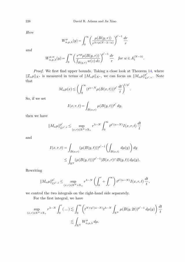
226 David R. Adams and Jie Xiao
Here
Wμα,p,λ(y) =
∫ ∞
0
(μ(B(y, r))
rλ+p(N −λ−α)
)p′ −1dr
r
and
Wμ,wα,p,λ(y) =
∫ ∞
0
(rαpμ(B(y, r))∫B(y,r)
w(z) dz
)p′ −1dr
rfor w ∈ A
(N −λ)1 .
Proof. We first find upper bounds. Taking a close look at Theorem 14, where‖Iαμ‖X∗ is measured in terms of ‖Mαμ‖X∗ , we can focus on ‖Mαμ‖p′
Lp′ ,λ . Notethat
Mαμ(x) ≤(∫ ∞
0
(tα−Nμ(B(x, t)))p′ dt
t
)1/p′
.
So, if we set
I(x, r, t) =∫
B(x,r)
μ(B(y, t))p′dy,
then we have
‖Mαμ‖p′
Lp′ ,λ ≤ sup(x,r)∈RN ×R+
rλ−N
∫ ∞
0
tp′(α−N)I(x, r, t)
dt
t
and
I(x, r, t) =∫
B(x,r)
(μ(B(y, t)))p′ −1
(∫B(x,t)
dμ(y))
dy
≤∫
RN
(μ(B(y, t)))p′ −1|B(x, r)∩B(y, t)| dμ(y).
Rewriting
‖Mαμ‖p′
Lp′ ,λ ≤ sup(x,r)∈RN ×R+
rλ−N
(∫ r
0
+∫ ∞
r
)tp
′(α−N)I(x, r, t)dt
t,
we control the two integrals on the right-hand side separately.For the first integral, we have
sup(x,r)∈RN ×R+
rλ−N
∫ r
0
( ... ) �∫ ∞
0
(tN+p′(α−N)tλ−N
∫RN
μ(B(y, 2t))p′ −1 dμ(y))
dt
t
�∫
RN
Wμα,p,λ dμ.
Morrey spaces in harmonic analysis 227
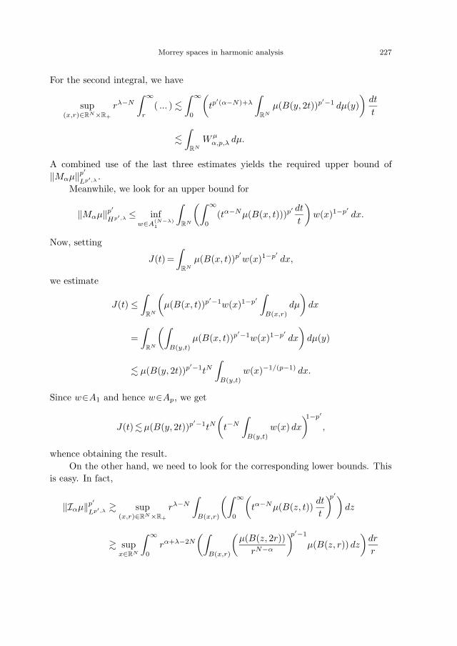
For the second integral, we have
sup(x,r)∈RN ×R+
rλ−N
∫ ∞
r
( ... ) �∫ ∞
0
(tp
′(α−N)+λ
∫RN
μ(B(y, 2t))p′ −1 dμ(y))
dt
t
�∫
RN
Wμα,p,λ dμ.
A combined use of the last three estimates yields the required upper bound of‖Mαμ‖p′
Lp′ ,λ .Meanwhile, we look for an upper bound for
‖Mαμ‖p′
Hp′ ,λ ≤ infw∈A
(N −λ)1
∫RN
(∫ ∞
0
(tα−Nμ(B(x, t)))p′ dt
t
)w(x)1−p′
dx.
Now, setting
J(t) =∫
RN
μ(B(x, t))p′w(x)1−p′
dx,
we estimate
J(t) ≤∫
RN
(μ(B(x, t))p′ −1w(x)1−p′
∫B(x,r)
dμ
)dx
=∫
RN
(∫B(y,t)
μ(B(x, t))p′ −1w(x)1−p′dx
)dμ(y)
� μ(B(y, 2t))p′ −1tN∫
B(y,t)
w(x)−1/(p−1) dx.
Since w ∈A1 and hence w ∈Ap, we get
J(t) �μ(B(y, 2t))p′ −1tN(
t−N
∫B(y,t)
w(x) dx
)1−p′
,
whence obtaining the result.On the other hand, we need to look for the corresponding lower bounds. This
is easy. In fact,
‖Iαμ‖p′
Lp′ ,λ � sup(x,r)∈RN ×R+
rλ−N
∫B(x,r)
(∫ ∞
0
(tα−Nμ(B(z, t))
dt
t
)p′ )dz
� supx∈RN
∫ ∞
0
rα+λ−2N
(∫B(x,r)
(μ(B(z, 2r))
rN −α
)p′ −1
μ(B(z, r)) dz
)dr
r

228 David R. Adams and Jie Xiao
�∫ ∞
0
rλ−NrNr(α−N)p′(∫
RN
μ(B(y, r))p′ −1 dμ(y))
dr
r
�∫
RN
Wμα,p,λ dμ.
And for the other, we have
‖Iαμ‖p′
Hp′ ,λ � infw∈A
(N −λ)1
∫RN
(∫ ∞
0
tα−Nμ(B(x, t))dt
t
)p′
w(x)1−p′dx
� infw∈A
(N −λ)1
∫ ∞
0
r(α−N)(1+p′)
∫RN
∫B(z,r)
w(x)1−p′dx(∫
B(z,3r)dμ(y)
)1−p′ dμ(z)dr
r
� infw∈A
(N −λ)1
∫RN
∫ ∞
0
r(α−N)p′
μ(B(z, r))1−p′
(∫B(z,r)
w(x)1−p′dx
)dr
rdμ(z)
� infw∈A
(N −λ)1
∫RN
∫ ∞
0
(r(αp−N)/(p−1)
μ(B(z, r))1/(1−p)
)(r−N
∫B(z,r)
w(y) dy)1/(p−1)
dr
rdμ(z)
� infw∈A
(N −λ)1
∫RN
Wμ,wα,p,λ dμ.
In the last two estimates we again invoke the Ap condition for w. �
Remark 22. Recall from [5, Theorem 4.5.4] that if
Wμα,p(y) =
∫ ∞
0
(μ(B(y, r)
)rN −αp
)1/(p−1)dr
r
is the so-called Wolff potential, then
‖ Iαμ‖p′
Lp′ ∼∫
RN
Wμα,p(y) dμ(y).
This type of estimate may be regarded as a special case λ=N of Theorem 21.
References
1. Adams, D. R., A note on Riesz potentials, Duke Math. J. 42 (1975), 765–778.2. Adams, D. R., Lecture Notes on Lp-Potential Theory, Dept. of Math., University of
Umea, Umea, 1981.

Morrey spaces in harmonic analysis 229
3. Adams, D. R., A note on Choquet integrals with respect to Hausdorff capacity, inFunction Spaces and Applications (Lund, 1986 ), Lecture Notes in Math. 1302,pp. 115–124, Springer, Berlin–Heidelberg, 1988.
4. Adams, D. R., Choquet integrals in potential theory, Publ. Mat. 42 (1998), 3–66.5. Adams, D. R. and Hedberg, L. I., Function Spaces and Potential Theory, Springer,
Berlin, 1996.6. Adams, D. R. and Xiao, J., Nonlinear analysis on Morrey spaces and their capacities,
Indiana Univ. Math. J. 53 (2004), 1629–1663.7. Alvarez, J., Continuity of Calderon–Zygmund type operators on the predual of a
Morrey space, in Clifford Algebras in Analysis and Related Topics (Fayetteville,AR, 1993 ), Stud. Adv. Math. 5, pp. 309–319, CRC, Boca Raton, FL, 1996.
8. Anger, B., Representation of capacities, Math. Ann. 229 (1977), 245–258.9. Bennett, C. and Sharpley, R., Interpolation of Operators, Pure and Applied Math.,
129, Academic Press, New York, 1988.10. Bensoussan, A. and Frehse, J., Regularity Results for Nonlinear Elliptic Systems
and Applications, Springer, Berlin, 2002.11. Blasco, O., Ruiz, A. and Vega, L., Non-interpolation in Morrey–Campanato and
block spaces, Ann. Sc. Norm. Super. Pisa Cl. Sci. 28 (1999), 31–40.12. Caffarelli, L. A., Salsa, S. and Silvestre, L., Regularity estimates for the solution
and the free boundary to the obstacle problem for the fractional Laplacian,Invent. Math. 171 (2008), 425–461.
13. Campanato, S., Proprieta di inclusione per spazi di Morrey, Ricerche Mat. 12 (1963),67–86.
14. Carleson, L., Selected Problems on Exceptional Sets, Van Nostrand, Princeton, NJ,1967.
15. Chiarenza, F. and Frasca, M., Morrey spaces and Hardy–Littlewood maximal func-tion, Rend. Mat. Appl. 7 (1988), 273–279.
16. Choquet, G., Theory of capacities, Ann. Inst. Fourier (Grenoble) 5 (1953–54), 131–295.
17. Duong, X., Xiao, J. and Yan, L. X., Old and new Morrey spaces with heat kernelbounds, J. Fourier Anal. Appl. 13 (2007), 87–111.
18. Heinonen, J., Kilpelainen, T. and Martio, O., Nonlinear Potential Theory of De-generate Elliptic Equations, 2nd ed., Dover, Mineola, NY, 2006.
19. John, F. and Nirenberg, L., On functions of bounded mean oscillation, Comm. PureAppl. Math. 14 (1961), 415–426.
20. Fefferman, C. and Stein, E. M., Hp spaces of several variables, Acta Math. 129(1972), 137–193.
21. Fefferman, R., A theory of entropy in Fourier analysis, Adv. Math. 30 (1978), 171–201.
22. Harrell II, E. M. and Yolcu, S. Y., Eigenvalue inequalities for Klein–Gordon op-erators, J. Funct. Anal. 256 (2009), 3977–3995.
23. Kalita, E. A., Dual Morrey spaces, Dokl. Akad. Nauk 361 (1998), 447–449 (Russian).English transl.: Dokl. Math. 58 (1998), 85–87.
24. Maly, J. and Ziemer, W. P., Fine Regularity of Solutions of Elliptic Partial Dif-ferential Equations, Math. Surveys and Monographs 51, Amer. Math. Soc.,Providence, RI, 1997.
230 David R. Adams and Jie Xiao: Morrey spaces in harmonic analysis
25. Maz′ya, V. G. and Verbitsky, I. E., Infinitesimal form boundedness and Trudinger’s
subordination for the Schrodinger operator, Invent. Math. 162 (2005), 81–136.26. Morrey, C. B., On the solutions of quasi-linear elliptic partial differential equations,
Trans. Amer. Math. Soc. 43 (1938), 126–166.27. Orobitg, J. and Verdera, J., Choquet integrals, Hausdorff content and the Hardy–
Littlewood maximal operator, Bull. Lond. Math. Soc. 30 (1998), 145–150.28. Peetre, J., On the theory of Lp,λ spaces, J. Funct. Anal. 4 (1969), 71–87.29. Ruiz, A. and Vega, L., Corrigenda to unique ..., and a remark on interpolation on
Morrey spaces, Publ. Mat. 39 (1995), 405–411.30. Sadosky, C., Interpolation of Operators and Singular Integrals, Pure and Appl. Math.,
Marcel Dekker, New York–Basel, 1979.31. Sarason, D., Functions of vanishing mean oscillation, Trans. Amer. Math. Soc. 207
(1975), 391–405.32. Stampacchia, G., The spaces L(p,λ), N (p,λ) and interpolation, Ann. Sc. Norm. Super.
Pisa 19 (1965), 443–462.33. Stein, E. M., Singular Integrals and Differentiability of Functions, Princeton Univ.
Press, Princeton, NJ, 1970.34. Stein, E. M., Harmonic Analysis: Real-variable Methods, Orthogonality, and Oscilla-
tory Integrals, Princeton Univ. Press, Princeton, NJ, 1993.35. Stein, E. M. and Zygmund, A., Boundedness of translation invariant operators on
Holder spaces and Lp-spaces, Ann. of Math. 85 (1967), 337–349.36. Taylor, M., Microlocal analysis on Morrey spaces, in Singularities and Oscilla-
tions (Minneapolis, MN, 1994/1995 ), IMA Vol. Math. Appl. 91, pp. 97–135,Springer, New York, 1997.
37. Torchinsky, A., Real-variable Methods in Harmonic Analysis, Dover, New York,2004.
38. Xiao, J., Homothetic variant of fractional Sobolev spaces with application to Navier–Stokes system, Dyn. Partial Differ. Equ. 4 (2007), 227–245.
39. Yang, D. and Yuan, W., A note on dyadic Hausdorff capacities, Bull. Sci. Math. 132(2008), 500–509.
40. Zorko, C. T., Morrey spaces, Proc. Amer. Math. Soc. 98 (1986), 586–592.
David R. AdamsDepartment of MathematicsUniversity of KentuckyLexington, KY [email protected]
Jie XiaoDepartment of Mathematics and StatisticsMemorial University of NewfoundlandSt. John’s, NL A1C [email protected]
Received July 6, 2010published online March 4, 2011


![archive.ymsc.tsinghua.edu.cnarchive.ymsc.tsinghua.edu.cn/pacm_download/188/8219... · 2019-11-01 · arXiv:1605.00342v2 [math.AG] 15 May 2016 LocalCalabi–YaumanifoldsoftypeÃand](https://img.pdfslide.us/doc/110x75/5ecaf1577f946210c54249a5/2019-11-01-arxiv160500342v2-mathag-15-may-2016-localcalabiayaumanifoldsoftypefand.jpg)