On the Optimal Thermal Management of Hybrid-Electric Vehicles

This paper is a part of the hereunder thematic dossierpublished in OGST Journal, Vol. 67, No. 4, pp. 539-645

and available online hereCet article fait partie du dossier thématique ci-dessous publié dans la revue OGST, Vol. 67, n°4, pp. 539-645

et téléchargeable ici

D o s s i e r

DOSSIER Edited by/Sous la direction de : A. Sciarretta

Electronic Intelligence in Vehicles

Intelligence électronique dans les véhiculesOil & Gas Science and Technology – Rev. IFP Energies nouvelles, Vol. 67 (2012), No. 4, pp. 539-645

Copyright © 2012, IFP Energies nouvelles

539 > Editorial

547 > Design and Optimization of Future Hybrid and Electric PropulsionSystems: An Advanced Tool Integrated in a Complete Workflow toStudy Electric DevicesDéveloppement et optimisation des futurs systèmes de propulsionhybride et électrique : un outil avancé et intégré dans une chaînecomplète dédiée à l’étude des composants électriquesF. Le Berr, A. Abdelli, D.-M. Postariu and R. Benlamine

563 > Sizing Stack and Battery of a Fuel Cell Hybrid Distribution TruckDimensionnement pile et batterie d’un camion hybride à pileà combustible de distributionE. Tazelaar, Y. Shen, P.A. Veenhuizen, T. Hofman and P.P.J. van den Bosch

575 > Intelligent Energy Management for Plug-in Hybrid Electric Vehicles:The Role of ITS Infrastructure in Vehicle ElectrificationGestion énergétique intelligente pour véhicules électriques hybridesrechargeables : rôle de l’infrastructure de systèmes de transportintelligents (STI) dans l’électrification des véhiculesV. Marano, G. Rizzoni, P. Tulpule, Q. Gong and H. Khayyam

589 > Evaluation of the Energy Efficiency of a Fleet of Electric Vehiclefor Eco-Driving ApplicationÉvaluation de l’efficacité énergétique d’une flotte de véhiculesélectriques dédiée à une application d’éco-conduiteW. Dib, A. Chasse, D. Di Domenico, P. Moulin and A. Sciarretta

601 > On the Optimal Thermal Management of Hybrid-Electric Vehicleswith Heat Recovery SystemsSur le thermo-management optimal d’un véhicule électriquehybride avec un système de récupération de chaleurF. Merz, A. Sciarretta, J.-C. Dabadie and L. Serrao

613 > Estimator for Charge Acceptance of Lead Acid BatteriesEstimateur d’acceptance de charge des batteries Pb-acideU. Christen, P. Romano and E. Karden

633 > Automatic-Control Challenges in Future Urban Vehicles: A Blendof Chassis, Energy and Networking ManagementLes défis de la commande automatique dans les futurs véhiculesurbains : un mélange de gestion de châssis, d’énergie et du réseauS.M. Savaresi

©Sh

utte

rsto

ck, a

rtic

le D

OI:

10.

2516

/ogs

t/201

2029

http://ogst.ifpenergiesnouvelles.fr/articles/ogst/abs/2012/04/contents/contents.html

http://ogst.ifpenergiesnouvelles.fr/articles/ogst/abs/2012/04/contents/contents.html

Oil & Gas Science and Technology – Rev. IFP Energies nouvelles, Vol. 67 (2012), No. 4, pp. 601-612Copyright c© 2012, IFP Energies nouvellesDOI: 10.2516/ogst/2012017

On the Optimal Thermal Managementof Hybrid-Electric Vehicles with Heat Recovery

SystemsF. Merz1, A. Sciarretta2∗, J.-C. Dabadie2 and L. Serrao2

1 ETH Zurich, Dept. of Mechanical and Process Engineering, Sonnegstr. 3, 8092 Zürich, Switzerland; now with the International PostgraduateTrainee, ZF Friedrichshafen AG, 88038 Friedrichshafen - Germany

2 IFP Energies nouvelles, 1-4 avenue de Bois-Préau, 92852 Rueil-Malmaison Cedex - Francee-mail: [email protected] (present address) - [email protected] - [email protected] -

[email protected] (present address)∗ Corresponding author

Résumé — Sur le thermo-management optimal d’un véhicule électrique hybride avec un sys-tème de récupération de chaleur — Une approche généralisée pour combiner la gestion de l’énergie(supervision du groupe motopropulseur) et le thermo-management dans les véhicules hybrides élec-triques est proposée. Un système hybride incluant le post-traitement des polluants et un système derécupération de la chaleur à l’échappement du moteur thermique est simulé pour plusieurs scénarii,y compris le cas de départ à froid. Des stratégies de gestion de l’énergie optimales sont dérivées àpartir du Principe de Minimum de Pontriaguine (PMP). Inspirée par les facteurs d’équivalence pour laconsommation électrique que l’on retrouve dans la stratégie ECMS, la notion d’équivalent en carbu-rant des flux d’énergie thermique est introduite. Les stratégies dérivées du PMP sont comparées avecune stratégie heuristique basée sur des règles. Les bénéfices en termes d’économies de carburant etréduction des émissions polluantes que l’on trouve pour différents scénarii sont encourageantes.

Abstract — On the Optimal Thermal Management of Hybrid-Electric Vehicles with Heat RecoverySystems — A general framework to combine optimal energy management (powertrain supervisorycontrol) and thermal management in Hybrid Electric Vehicles (HEV) is presented. A HEV system withengine exhaust aftertreatment and exhaust heat recovery system is simulated under various scenarios,including warm and cold start. Optimal strategies are derived from Pontryagin Minimum Principle(PMP). The concept of fuel equivalent of thermal energy variations – similar to the equivalencefactors for battery energy of standard Equivalent Consumption Minimization Strategy (ECMS) – isintroduced. The PMP-based strategies are compared with a heuristic, rule-based strategy. The benefitsin fuel economy and reduction of pollutant emissions that are obtained for several scenarios are verypromising.

INTRODUCTION

The contribution of hybrid-electric powertrain technology tofuture mobility is expected to grow. On one hand, suchpropulsion systems can improve the rather poor thermalefficiency of standard internal-combustion engines. On theother hand, they pave the way to a partial electrification

of individual mobility by combining short-range purelyelectric travel with long range driving capability (plug-in and extended-range concepts). One distinguishing fea-ture of HEVs is the need for a nontrivial energy manage-ment strategy in order to control the energy flow withinthe vehicle. This supervisory control task has attracted aconsiderable amount of research in the last fifteen years

Articles LAtexttdecoupe_06-ogst110046latex2 04/10/12 12:01 Page1

D o s s i e rElectronic Intelligence in Vehicles

Intelligence électronique dans les véhicules

http://ogst.ifpenergiesnouvelles.fr

http://ifpenergiesnouvelles.fr

http://ogst.ifp.fr/articles/ogst/abs/2012/04/contents/contents.html

602 Oil & Gas Science and Technology – Rev. IFP Energies nouvelles, Vol. 67 (2012), No. 4

(surveys [1-3]). Common energy management strategies arebased on heuristic considerations inspired by the expectedbehavior of the propulsion system. Moreover, optimizedstrategies have been introduced that are based on thedefinition of a cost function to be minimized and optimalcontrol to achieve it. The offline version of this paradigmis widely used in the automotive industry to assess the per-formance of various solutions and to pre-calibrate the onlineenergy management strategies [4-8]. State-of-the-art meth-ods for offline optimization of energy management strate-gies are dynamic programming and the direct application ofPontryagin’s minimum principle (PMP). The optimizationproblem is usually formulated as follows:

– the cost function is either fuel consumption or engine-out emissions, or a combination of both [9-11], althoughin [12] the battery ageing has been considered as well;

– the only system dynamics considered are those of thebattery State of Charge (SOC);

– the global constraint to the state variable reflects charge-sustaining (final SOC equals initial SOC) or charge-depleting (final SOC is nearly zero [13]) operation.

Recent works have been aimed at extending the stan-dard optimization problem to consider additional scenarios,including multiple electric sources [14, 15], drivability con-straints [16, 17] and additional dynamics. Indeed the HEVsystem has other dynamics than SOC that may be relevantfor overall optimization. The most important is obviouslythe vehicle longitudinal dynamics and thus vehicle speed.However, its optimization is usually out of the scope ofenergy management and rather concerns look-ahead drivecontrol (or predictive cruise control) [18, 19]. Next in rele-vance (and the object of this paper) are temperature levels,since thermal phenomena have longer characteristic timesthan mechanical or electrical phenomena. Temperature is akey factor in many phenomena:

– engine warm-up: fuel consumption and engine-out emis-sions depend on temperature levels (oil, coolant, block);

– engine cool-down: in HEVs the engine can be turned offand as a result its temperature decreases;

– activation (light-off) of the catalytic converter: effectiveconversion requires a certain threshold temperature; cat-alyst temperature dynamics are correlated with those ofthe engine;

– heat supplies to cabin heater or other uses (demist,defrost);

– heat accumulation systems (tanks, phase-changematerials);

– heat recovery systems (Rankine-cycles,thermoelectricity).

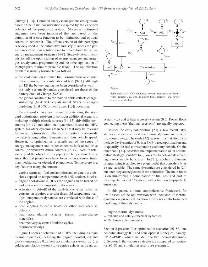
Figure 1 shows a schematic of a HEV including its mainthermal dynamics, including the engine (coolant, oil andblock) temperature θe, a heat accumulation system (θacc), acold accumulation system (θa/c) engine exhaust and catalyst

Pch, f

Pth,ec

Pth,ePth,aux

θc ξ

Pel,aux

θe

θacc

νveh

Pme,auxP f r,a/c

θa/ c

θr

Pth,cr Pel,r

Pel,m

Pme,v

MOT

RECCAT

ENG

A/C Transmission

Figure 1

Schematics of a HEV depicting relevant dynamics as "reser-voirs" (circles), as well as power flows (arrows) and powerconverters (blocks).

system (θc) and a heat recovery system (θr). Power flowsconnecting these "thermal reservoirs" are equally depicted.

Besides the early contribution [20], a few recent HEVstudies considered at least one thermal dynamic in the opti-mization strategy. The study [22] represents a first attempt toinclude the dynamics of θe in a PMP-based optimization andto quantify the fuel corresponding economy benefit. On theother hand [23], describes the implementation of an optimalonline strategy, sensitive to θc, on a test bench and its advan-tages over simple heuristics. In [21], stochastic dynamicprogramming is applied to a plant model that considers θc asa state variable. The same dynamics are considered in [24]but later they are neglected in the controller. The main focusis on minimizing a combination of fuel cost and cost ofurea injected in a SCR system, with a limit on tailpipe NOx

emission.

In this paper, a more comprehensive framework forPMP-based offline optimization with inclusion of thermaldynamics is presented. Section 1 presents control-orientedmodeling of three dynamics:

– engine thermal dynamics;– exhaust and catalyst thermal dynamics;– Rankine-cycle dynamics.

Section 2 presents four optimization scenarios S0–S3, oneheuristic strategy RB and four optimal strategies, namely,PMP0–PMP3, which include up to two thermal dynamics.In Section 3, the various strategies are compared for scenar-ios S0–S3 and simulation results are presented.


F. Merz et al. / On the Optimal Thermal Management of Hybrid-Electric Vehicles with Heat Recovery Systems 603

1 MODELING

1.1 Full-Order Model (FOM)

The system considered here is a combined (power-split)hybrid vehicle (1 360 kg curb weight) equipped with a70 kW gasoline engine, two motors/generators (50 kWand 30 kW) and a 6.9 Ah Li-ion battery. A detailedmodel of the system was developed and implemented inAMESim [25] (1). The detailed model, labelled here asFOM (Full-Order Model), simulates the mechanical, elec-trical and thermal phenomena in the HEV, including driverresponse, combustion mode, temperature corrections forfuel consumption and engine-out emissions, engine torqueresponse, engine control loop dynamics, inertia of electricmachines, thermal capacity of engine oil, engine coolant cir-cuit, external cooling circuit with radiator and heat exchang-ers, exhaust system including three-way catalytic converter,cabin heater and electric auxiliaries. The submodels of var-ious components are linked with each other based on theirmechanical, electrical, thermal couplings and on the basis ofa physical ("forward") causality.

Due to its comprehensive nature and complexity, theFOM is impractical for control and optimization pur-poses. Instead, a reduced-order counterpart (ROM) has beenderived. Generally speaking, the main thermal dynamics areapproximated by lumped temperature levels, while all of theother dynamics are neglected and the corresponding staticrelationships are used. The choice of the thermal levelsto consider depends on the particular optimization scenariounder study. Three cases are described in the following sub-sections.

1.2 Engine Temperature

The effect of engine temperature on the fuel consumptionrate m f is modeled in the ROM as:

m f (u, θe) = m◦f (u) · fcons(u, θe) (1)

where u is the engine operating point (see below), fcons(·)is an extra-consumption factor that takes into account theincrease of friction and the increase of fuel injected per cycleat low temperatures. Data for warm-engine fuel consump-tion m◦f are derived from engine tests and implemented in thesame way as in the FOM. Data for fcons are derived from:– extra injection rate tabulated as a function of coolant tem-

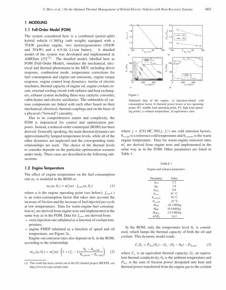
perature;– engine FMEP tabulated as a function of speed and oil

temperature, see Figure 2a.Engine-out emission rates also depend on θe in the ROM,

according to the relationship:

m j,e(u, θe) = m◦j(u) ·(1 + ( f j − 1)

θe − θe,cold

θe,warm − θe,cold

)(2)

(1) This work has been carried out in the EU-funded project HICEPS, seehttp://www.hi-ceps.eu/tutto.htm

−50 0 50 1001.0

1.2

1.4

1.6

1.8

−50 0 50 1000.5

1.0

1.5

2.0

2.5

100 100200 200300 30040

0

400

500

500

600

600

700

700

800

0 200 4000

50

100 1

11

1

1

1.1

1.1

0 200 4000

50

100

f con

s(-

)

θe (◦C)a)

θe (◦C)b)

Te

(Nm

)

Te

(Nm

)

Te,max

Te,max

θexh

ωe (rad/s)c)

ωe (rad/s)d)

Pth,e/P

me,

e

φ

P1P2

Figure 2

Tabulated data of the engine, a) injection-related coldconsumption factor, b) thermal power losses at two operatingpoints (P1: middle-load operating point, P2: high-load operat-ing point), c) exhaust temperature, d) equivalence ratio.

where j = {CO,HC,NOx}, f j’s are cold emission factors,θe,cold is a reference cold temperature and θe,warm is the warmengine temperature. Data for warm-engine emission ratesm◦j are derived from engine tests and implemented in thesame way as in the FOM. Other parameters are listed inTable 1.

TABLE 1

Engine and exhaust parameters

Parameter ValuefCO 2.2fHC 1.8fNOx 0.8θe,∞ 87 ◦Cθe,warm 70 ◦Cθe,cold -25 ◦CHCO -10.1 MJ/kgHHC 45.8 MJ/kgHNOx -12.5 MJ/kgAFRst 14.5

In the ROM, only the temperature level θe is consid-ered, which lumps the thermal capacity of both the oil andcoolant. This dynamic model reads:

Ceθe = Pth,e(θe) −Ge · (θe − θ0) − Pth,aux (3)

where Ce is an equivalent thermal capacity, Ge an equiva-lent thermal conductivity, θ0 is the ambient temperature andPth,e is the sum of friction power dissipated into heat andthermal power transferred from the engine gas to the coolant



0 200 400 600 800 1 000 1 2000

100

200

300

400

0 200 400 600 800 1 000 1 2000

50

100

150

θe

(◦C

)M

f(g

)

t (s)a)

t (s)b)

FOM

FOM

ROM

ROM

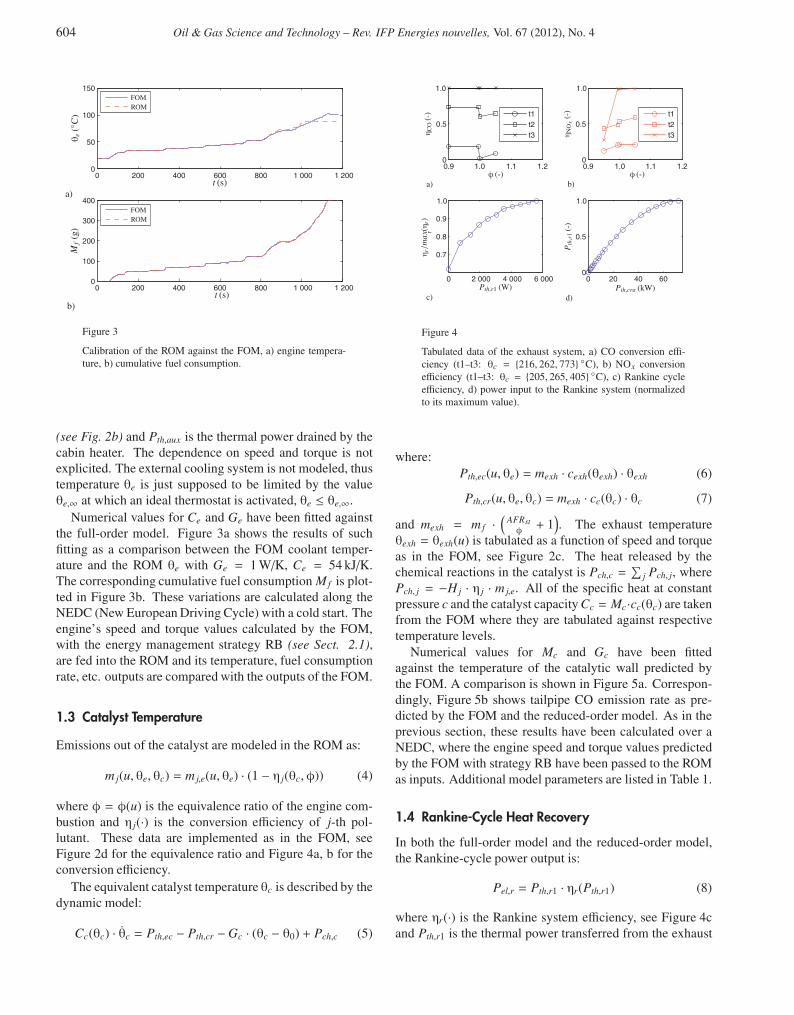
Figure 3

Calibration of the ROM against the FOM, a) engine tempera-ture, b) cumulative fuel consumption.

(see Fig. 2b) and Pth,aux is the thermal power drained by thecabin heater. The dependence on speed and torque is notexplicited. The external cooling system is not modeled, thustemperature θe is just supposed to be limited by the valueθe,∞ at which an ideal thermostat is activated, θe ≤ θe,∞.

Numerical values for Ce and Ge have been fitted againstthe full-order model. Figure 3a shows the results of suchfitting as a comparison between the FOM coolant temper-ature and the ROM θe with Ge = 1 W/K, Ce = 54 kJ/K.The corresponding cumulative fuel consumption M f is plot-ted in Figure 3b. These variations are calculated along theNEDC (New European Driving Cycle) with a cold start. Theengine’s speed and torque values calculated by the FOM,with the energy management strategy RB (see Sect. 2.1),are fed into the ROM and its temperature, fuel consumptionrate, etc. outputs are compared with the outputs of the FOM.

1.3 Catalyst Temperature

Emissions out of the catalyst are modeled in the ROM as:

m j(u, θe, θc) = m j,e(u, θe) · (1 − η j(θc,φ)) (4)

where φ = φ(u) is the equivalence ratio of the engine com-bustion and η j(·) is the conversion efficiency of j-th pol-lutant. These data are implemented as in the FOM, seeFigure 2d for the equivalence ratio and Figure 4a, b for theconversion efficiency.

The equivalent catalyst temperature θc is described by thedynamic model:

Cc(θc) · θc = Pth,ec − Pth,cr −Gc · (θc − θ0) + Pch,c (5)

0.9 1.0 1.1 1.20

0.5

1.0

t1t2t3

0.9 1.0 1.1 1.20

0.5

1.0

t1t2t3

0 2 000 4 000 6 000

0.7

0.8

0.9

1.0

r

0 20 40 600

0.5

1.0

φ (-)a)

φ (-)b)

ηC

O(-

)η

r/m

ax(η

r)

ηN

Ox

(-)

Pth,r1 (W)c)

Pth,cra (kW)d)

Pth,r

1(-

)

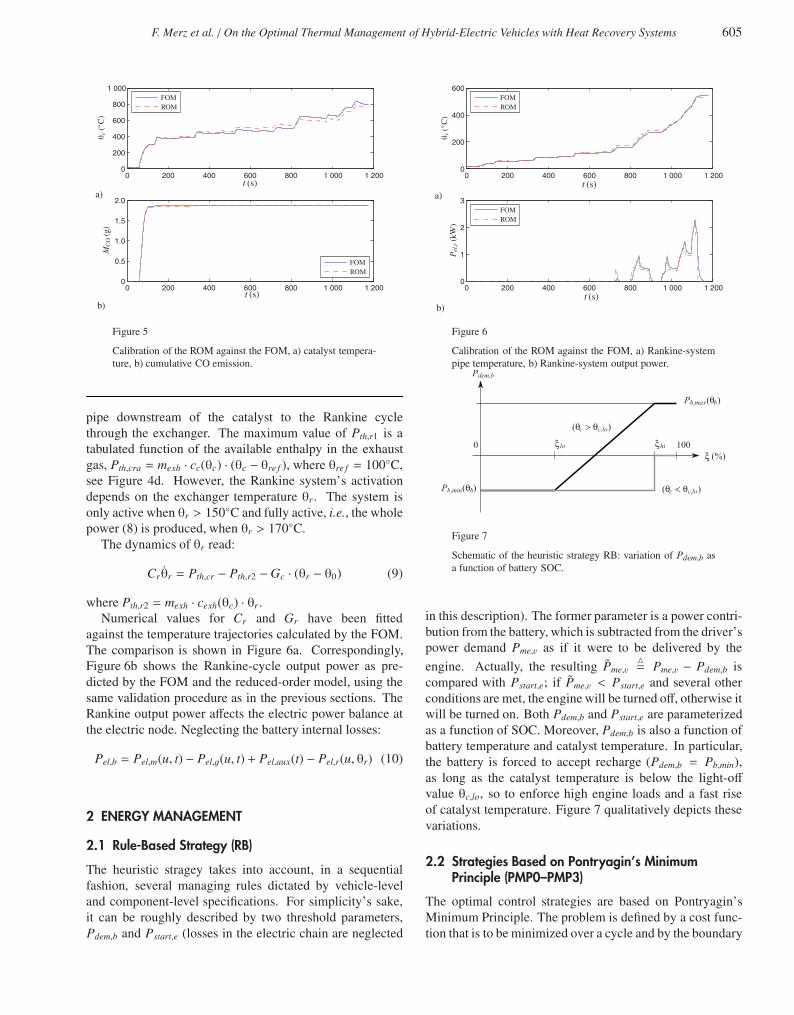
Figure 4

Tabulated data of the exhaust system, a) CO conversion effi-ciency (t1–t3: θc = {216, 262, 773} ◦C), b) NOx conversionefficiency (t1–t3: θc = {205, 265, 405} ◦C), c) Rankine cycleefficiency, d) power input to the Rankine system (normalizedto its maximum value).

where:Pth,ec(u, θe) = mexh · cexh(θexh) · θexh (6)

Pth,cr(u, θe, θc) = mexh · cc(θc) · θc (7)

and mexh = m f ·(

AFRstφ+ 1). The exhaust temperature

θexh = θexh(u) is tabulated as a function of speed and torqueas in the FOM, see Figure 2c. The heat released by thechemical reactions in the catalyst is Pch,c =

∑j Pch, j, where

Pch, j = −H j · η j · m j,e. All of the specific heat at constantpressure c and the catalyst capacity Cc = Mc·cc(θc) are takenfrom the FOM where they are tabulated against respectivetemperature levels.

Numerical values for Mc and Gc have been fittedagainst the temperature of the catalytic wall predicted bythe FOM. A comparison is shown in Figure 5a. Correspon-dingly, Figure 5b shows tailpipe CO emission rate as pre-dicted by the FOM and the reduced-order model. As in theprevious section, these results have been calculated over aNEDC, where the engine speed and torque values predictedby the FOM with strategy RB have been passed to the ROMas inputs. Additional model parameters are listed in Table 1.

1.4 Rankine-Cycle Heat Recovery

In both the full-order model and the reduced-order model,the Rankine-cycle power output is:

Pel,r = Pth,r1 · ηr(Pth,r1) (8)

where ηr(·) is the Rankine system efficiency, see Figure 4cand Pth,r1 is the thermal power transferred from the exhaust



0 200 400 600 800 1 000 1 2000

200

400

600

800

1 000

0 200 400 600 800 1 000 1 2000

0.5

1.0

1.5

2.0

t (s)a)

t (s)b)

FOM

FOM

ROM

ROMθ

c(◦

C)

MC

O(g

)

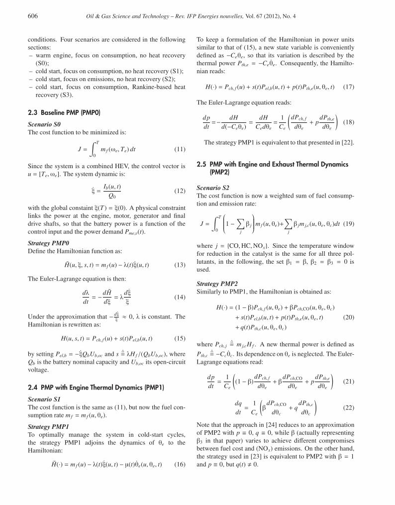
Figure 5

Calibration of the ROM against the FOM, a) catalyst tempera-ture, b) cumulative CO emission.

pipe downstream of the catalyst to the Rankine cyclethrough the exchanger. The maximum value of Pth,r1 is atabulated function of the available enthalpy in the exhaustgas, Pth,cra = mexh · cc(θc) · (θc − θre f ), where θre f = 100◦C,see Figure 4d. However, the Rankine system’s activationdepends on the exchanger temperature θr . The system isonly active when θr > 150◦C and fully active, i.e., the wholepower (8) is produced, when θr > 170◦C.

The dynamics of θr read:

Crθr = Pth,cr − Pth,r2 −Gc · (θr − θ0) (9)

where Pth,r2 = mexh · cexh(θc) · θr .Numerical values for Cr and Gr have been fitted

against the temperature trajectories calculated by the FOM.The comparison is shown in Figure 6a. Correspondingly,Figure 6b shows the Rankine-cycle output power as pre-dicted by the FOM and the reduced-order model, using thesame validation procedure as in the previous sections. TheRankine output power affects the electric power balance atthe electric node. Neglecting the battery internal losses:

Pel,b = Pel,m(u, t) − Pel,g(u, t) + Pel,aux(t) − Pel,r(u, θr) (10)

2 ENERGY MANAGEMENT

2.1 Rule-Based Strategy (RB)

The heuristic stragey takes into account, in a sequentialfashion, several managing rules dictated by vehicle-leveland component-level specifications. For simplicity’s sake,it can be roughly described by two threshold parameters,Pdem,b and Pstart,e (losses in the electric chain are neglected

0 200 400 600 800 1 000 1 2000

200

400

600

0 200 400 600 800 1 000 1 2000

1

2

3

t (s)a)

t (s)b)

FOM

FOM

ROM

ROM

θr

(◦C

)P

el,r

(kW

)

Figure 6

Calibration of the ROM against the FOM, a) Rankine-systempipe temperature, b) Rankine-system output power.

Pdem,b

ξ lo ξhi

Pb,min(θb)

Pb,max(θb)

ξ (%)0 100

(θc > θc,lo)

(θc < θc,lo)

Figure 7

Schematic of the heuristic strategy RB: variation of Pdem,b asa function of battery SOC.

in this description). The former parameter is a power contri-bution from the battery, which is subtracted from the driver’spower demand Pme,v as if it were to be delivered by the

engine. Actually, the resulting Pme,v�= Pme,v − Pdem,b is

compared with Pstart,e; if Pme,v < Pstart,e and several otherconditions are met, the engine will be turned off, otherwise itwill be turned on. Both Pdem,b and Pstart,e are parameterizedas a function of SOC. Moreover, Pdem,b is also a function ofbattery temperature and catalyst temperature. In particular,the battery is forced to accept recharge (Pdem,b = Pb,min),as long as the catalyst temperature is below the light-offvalue θc,lo, so to enforce high engine loads and a fast riseof catalyst temperature. Figure 7 qualitatively depicts thesevariations.

2.2 Strategies Based on Pontryagin’s MinimumPrinciple (PMP0–PMP3)

The optimal control strategies are based on Pontryagin’sMinimum Principle. The problem is defined by a cost func-tion that is to be minimized over a cycle and by the boundary



conditions. Four scenarios are considered in the followingsections:– warm engine, focus on consumption, no heat recovery

(S0);– cold start, focus on consumption, no heat recovery (S1);– cold start, focus on emissions, no heat recovery (S2);– cold start, focus on consumption, Rankine-based heat

recovery (S3).

2.3 Baseline PMP (PMP0)

Scenario S0The cost function to be minimized is:

J =∫ T

0m f (ωe, Te) dt (11)

Since the system is a combined HEV, the control vector isu = [Te,ωe]. The system dynamic is:

ξ =Ib(u, t)

Q0(12)

with the global constaint ξ(T ) = ξ(0). A physical constraintlinks the power at the engine, motor, generator and finaldrive shafts, so that the battery power is a function of thecontrol input and the power demand Pme,v(t).

Strategy PMP0Define the Hamiltonian function as:

H(u, ξ, s, t) = m f (u) − λ(t)ξ(u, t) (13)

The Euler-Lagrange equation is then:

dλdt= −dH

dξ= λ

dξξ

(14)

Under the approximation that − dξξ≈ 0, λ is constant. The

Hamiltonian is rewritten as:

H(u, s, t) = Pch, f (u) + s(t)Pel,b(u, t) (15)

by setting Pel,b = −ξQbUb,oc and s�= λH f /(QbUb,oc), where

Qb is the battery nominal capacity and Ub,oc its open-circuitvoltage.

2.4 PMP with Engine Thermal Dynamics (PMP1)

Scenario S1The cost function is the same as (11), but now the fuel con-sumption rate m f = m f (u, θe).

Strategy PMP1To optimally manage the system in cold-start cycles,the strategy PMP1 adjoins the dynamics of θe to theHamiltonian:

H(·) = m f (u) − λ(t)ξ(u, t) − µ(t)θe(u, θe, t) (16)

To keep a formulation of the Hamiltonian in power unitssimilar to that of (15), a new state variable is convenientlydefined as −Ceθe, so that its variation is described by thethermal power Pth,e = −Ceθe. Consequently, the Hamilto-nian reads:

H(·) = Pch, f (u) + s(t)Pel,b(u, t) + p(t)Pth,e(u, θe, t) (17)

The Euler-Lagrange equation reads:

dpdt=−

dHd(−Ceθe)

=dH

Cedθe=

1Ce

(dPch, f

dθe+ p

dPth,e

dθe

)(18)

The strategy PMP1 is equivalent to that presented in [22].

2.5 PMP with Engine and Exhaust Thermal Dynamics(PMP2)

Scenario S2The cost function is now a weighted sum of fuel consump-tion and emission rate:

J =∫ T

0

1 −∑

j

β j

m f (u, θe)+∑

j

β jm j,c(u, θe, θc)dt (19)

where j = {CO,HC,NOx}. Since the temperature windowfor reduction in the catalyst is the same for all three pol-lutants, in the following, the set β1 = β, β2 = β3 = 0 isused.

Strategy PMP2Similarly to PMP1, the Hamiltonian is obtained as:

H(·) = (1 − β)Pch, f (u, θe) + βPch,CO(u, θe, θc)

+ s(t)Pel,b(u, t) + p(t)Pth,e(u, θe, t) (20)

+ q(t)Pth,c(u, θe, θc)

where Pch, j�= m j,cH f . A new thermal power is defined as

Pth,c�= −Ccθc. Its dependence on θe is neglected. The Euler-

Lagrange equations read:

dpdt=

1Ce

((1 − β)

dPch, f

dθe+ β

dPch,CO

dθe+ p

dPth,e

dθe

)(21)

dqdt=

1Ce

(β

dPch,CO

dθc+ q

dPth,c

dθc

)(22)

Note that the approach in [24] reduces to an approximationof PMP2 with p ≡ 0, q ≡ 0, while β (actually representingβ3 in that paper) varies to achieve different compromisesbetween fuel cost and (NOx) emissions. On the other hand,the strategy used in [23] is equivalent to PMP2 with β = 1and p ≡ 0, but q(t) � 0.



2.6 PMP with Engine, Exhaust and Heat RecoveryDynamics (PMP3)

Scenario S3Cost function as in S1.

Strategy PMP3The Hamiltonian reads:

H(·) = Pch, f (u) + s(t)Pel,b(u, t) +

p(t)Pth,e(u, θe, t) + r(t)Pth,r(u, θr) (23)

where Pth,r�= −Crθr . The Euler-Lagrange equations read:

dpdt=

1Ce

(dPch, f

dθe+ p

dPth,e

dθe

)(24)

drdt=

1Cr

(−dPel,r

dθr+ r

dPth,r

dθr

)(25)

3 SIMULATION RESULTS

In this section, results of HOT simulation runs for scenar-ios S0–S3 are presented and compared with strategy RB.Scenario definitions are listed in Table 2. In particular, fueleconomy, emissions, SOC variations and temperature varia-tions are analyzed. In order to compare different trajectoriesleading to different values of final SOC, fuel economy dataare corrected to take into account overall SOC deviationswith respect to the initial value. Corrected fuel economyis found by interpolation between actual runs with oppositeSOC balance or using the equivalence factor s to convertresidual electrochemical energy into fuel.

TABLE 2

Definition of test scenarios S0–S3, with respect to a Cold Start (CS), thevalue of β, the presence of a Rankine System (RS). Y/N: Yes/no.

Scenario CS β RSS0 N 1 NS1 Y 0 NS2a Y 1 NS2b Y 0.25 NS3 Y 1 Y

3.1 Hybrid Optimization Tool (HOT)

The optimal strategies are calculated with the software HOT(Hybrid Optimization Tool) developed at IFP Energies Nou-velles and presented, e.g., in [26]. HOT uses a genericHEV structure that can be parameterized to represent var-ious hybrid architectures, including the combined architec-ture of the system considered here. Until the 2011 version,only strategy PMP0 was applied. The optimal value of theequivalence factor s is found using the bisection method. Anew feature introduced in 2011 includes the possibility ofsetting strategies PMP1 to PMP3.

200 400 600 800 1 000 1 200−20

20

40

200 400 600 800 1 000 1 20035

40

45

50

55

ξ(%

)

t (s)a)

t (s)b)

Pm

e,e

(kW

)

PMP0

PMP0

RB

RB

0

0

0

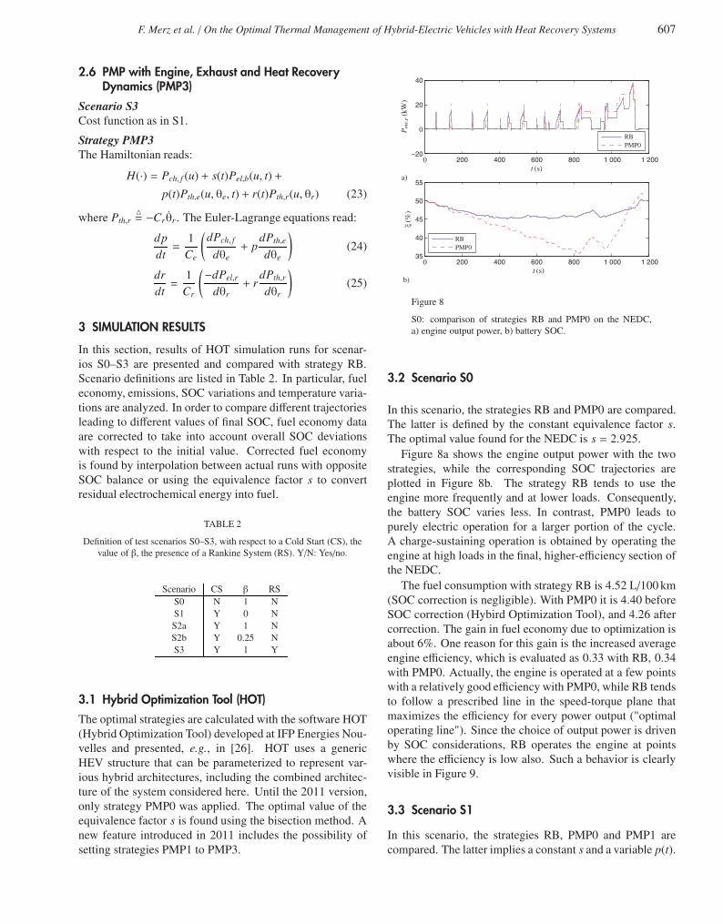
Figure 8

S0: comparison of strategies RB and PMP0 on the NEDC,a) engine output power, b) battery SOC.

3.2 Scenario S0

In this scenario, the strategies RB and PMP0 are compared.The latter is defined by the constant equivalence factor s.The optimal value found for the NEDC is s = 2.925.

Figure 8a shows the engine output power with the twostrategies, while the corresponding SOC trajectories areplotted in Figure 8b. The strategy RB tends to use theengine more frequently and at lower loads. Consequently,the battery SOC varies less. In contrast, PMP0 leads topurely electric operation for a larger portion of the cycle.A charge-sustaining operation is obtained by operating theengine at high loads in the final, higher-efficiency section ofthe NEDC.

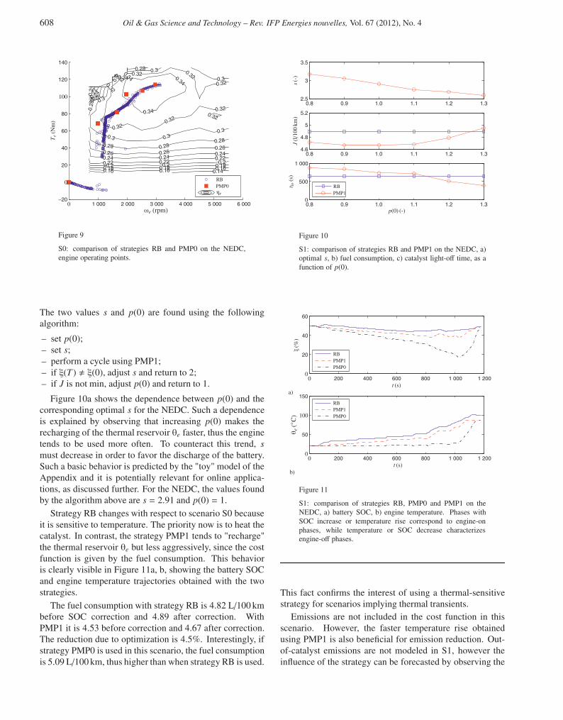
The fuel consumption with strategy RB is 4.52 L/100 km(SOC correction is negligible). With PMP0 it is 4.40 beforeSOC correction (Hybird Optimization Tool), and 4.26 aftercorrection. The gain in fuel economy due to optimization isabout 6%. One reason for this gain is the increased averageengine efficiency, which is evaluated as 0.33 with RB, 0.34with PMP0. Actually, the engine is operated at a few pointswith a relatively good efficiency with PMP0, while RB tendsto follow a prescribed line in the speed-torque plane thatmaximizes the efficiency for every power output ("optimaloperating line"). Since the choice of output power is drivenby SOC considerations, RB operates the engine at pointswhere the efficiency is low also. Such a behavior is clearlyvisible in Figure 9.

3.3 Scenario S1

In this scenario, the strategies RB, PMP0 and PMP1 arecompared. The latter implies a constant s and a variable p(t).



1 000 2 000 3 000 4 000 5 000 6 000−20

20

40

60

80

120

140

0.140.16 0.16 0.160.18 0.18 0.18

0.2

0.2 0.2 0.2

0.22

0.22 0.220.22

0.24

0.24 0.240.24

0.26

0.26 0.260.26

0.28

0.28 0.280.28

0.28

0.3

0.3 0.30.3

0.3

0.30.3

0.32

0.320.32

0.32

0.32 0.32

0.32

0.32

0.320.34

0.34

0.34

0.34

100

ηe

Te

(Nm

)

ωe (rpm)

PMP0RB0

0

Figure 9

S0: comparison of strategies RB and PMP0 on the NEDC,engine operating points.

The two values s and p(0) are found using the followingalgorithm:

– set p(0);– set s;– perform a cycle using PMP1;– if ξ(T ) � ξ(0), adjust s and return to 2;– if J is not min, adjust p(0) and return to 1.

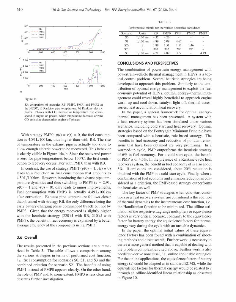
Figure 10a shows the dependence between p(0) and thecorresponding optimal s for the NEDC. Such a dependenceis explained by observing that increasing p(0) makes therecharging of the thermal reservoir θe faster, thus the enginetends to be used more often. To counteract this trend, smust decrease in order to favor the discharge of the battery.Such a basic behavior is predicted by the "toy" model of theAppendix and it is potentially relevant for online applica-tions, as discussed further. For the NEDC, the values foundby the algorithm above are s = 2.91 and p(0) = 1.

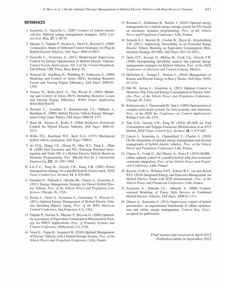
Strategy RB changes with respect to scenario S0 becauseit is sensitive to temperature. The priority now is to heat thecatalyst. In contrast, the strategy PMP1 tends to "recharge"the thermal reservoir θe but less aggressively, since the costfunction is given by the fuel consumption. This behavioris clearly visible in Figure 11a, b, showing the battery SOCand engine temperature trajectories obtained with the twostrategies.

The fuel consumption with strategy RB is 4.82 L/100 kmbefore SOC correction and 4.89 after correction. WithPMP1 it is 4.53 before correction and 4.67 after correction.The reduction due to optimization is 4.5%. Interestingly, ifstrategy PMP0 is used in this scenario, the fuel consumptionis 5.09 L/100 km, thus higher than when strategy RB is used.

0.8 0.9 1.0 1.1 1.2 1.32.5

3

3.5

0.8 0.9 1.0 1.1 1.2 1.34.6

4.8

5

5.2

0.8 0.9 1.0 1.1 1.2 1.3

500

1 000

p(0) (-)

s(-)

t lo(s

)J

(l/1

00km

)

RBPMP1

0

Figure 10

S1: comparison of strategies RB and PMP1 on the NEDC, a)optimal s, b) fuel consumption, c) catalyst light-off time, as afunction of p(0).

200 400 600 800 1 000 1 200

20

40

60

200 400 600 800 1 000 1 200

50

150

θe

(◦C

)ξ

(%)

00

00

PMP1

PMP1

PMP0

PMP0

t (s)a)

t (s)b)

RB

RB

100

Figure 11

S1: comparison of strategies RB, PMP0 and PMP1 on theNEDC, a) battery SOC, b) engine temperature. Phases withSOC increase or temperature rise correspond to engine-onphases, while temperature or SOC decrease characterizesengine-off phases.

This fact confirms the interest of using a thermal-sensitivestrategy for scenarios implying thermal transients.

Emissions are not included in the cost function in thisscenario. However, the faster temperature rise obtainedusing PMP1 is also beneficial for emission reduction. Out-of-catalyst emissions are not modeled in S1, however theinfluence of the strategy can be forecasted by observing the



warm-up time twu, defined operatively as the time at whichθe = 45◦C. Figure 10c shows that the twu decreases for anincrease of p(0). Using the calibration p(0) = 1 that opti-mizes fuel consumption, the warm-up time is reduced withrespect to PMP0 and thus the tailpipe emissions are likely tobe reduced as well.

3.4 Scenario S2

In this scenario, strategy RB’s behavior is the same as inscenario S1. The fuel consumption on the NEDC is 4.89 L/100 km and the CO emission is 1.88 g.

The behavior of strategy PMP2 is dependent on thechoice of β. The case β = 1 (minimization of the emis-sion) is considered first. As a basis of comparison, strat-egy PMP0 with an equivalence factor s = 0.28 would leadto a CO emission of 1.51 g. This result is obtained byconcentrating the engine-on phase toward the last part of thecycle, rather than speeding up the rise of catalyst temper-ature, see Figure 12a, b. Using strategy PMP1 (q(t) ≡ 0),a result virtually identical to PMP0 is obtained, which issymptomatic of the engine temperature’s relatively weakinfluence on the tailpipe emissions.

A slightly better result of 1.46 g is obtained using thestrategy PMP2 and p(t) ≡ 0, for example by settingq(0) = −0.1 and s = 50. Now the strategy starts the engine atthe very beginning of the cycle, when the vehicle is stopped,see Figure 12a, b. The power produced is partially chargedinto the battery, while the temperature of the catalyst risesrapidly. After this phase, the engine is kept off during therest of the cycle. Using the complete PMP2 strategy, forexample with p(0) = 0, q(0) = 0, the results are virtuallyidentical.

For β = 0.25 (minimization of a weighted sum of fuelconsumption and emissions), the cost function with strat-egy RB is 303 g. Despite its neglection of relevant dynam-ics, strategy PMP0 is already capable of attaining a similarresult. With a choice s = 2.965 (and p(t) = q(t) ≡ 0),1.67 g of CO and 4.87 L/100 km of fuel (corresponding to402 g) are obtained, with a cost function of 302 g. Again,this result is obtained by limiting the engine-on phases andconcentrating them toward the end of the cycle, rather thanfastening the rise of catalyst temperature, since PMP0 is nottemperature-sensitive (see Fig. 13a, b).

With PMP1 (q(t) ≡ 0), a slightly better result is obtainedwith p(0) = 0.8, s = 2.125, namely, 2.15 g CO and 395 gof fuel (4.78 L/100 km) for a cost function of 296 g. Withrespect to the previous case with β = 1, fuel consumption isnow included in the cost function and it is dependent on θe,from whence the positive effect given by the introductionof such dynamics in the Hamiltonian. Indeed, the patternof engine-on phases resembles that of PMP1 in scenario S1,Figure 11a. The rise of temperature is faster than with PMP0but less aggressive than with RB. By switching to strategyPMP2, no further improvement has been found.

200 400 600 800 1 000 1 200

200

400

600

800

1 000

200 400 600 800 1 000 1 200

0.5

1

1.5

2

RB

RB

00

00

PMP0

PMP0

PMP2

PMP2

t (s)a)

t (s)b)

θc

(◦C

)M

CO

(g)

Figure 12

S2: comparison of strategies RB, PMP0, and PMP2 (β = 1)on the NEDC, a) catalyst temperature, b) cumulative CO emis-sion. Phases with CO increase or temperature rise correspondto engine-on phases, while temperature decrease or zero COemission characterize engine-off phases.

200 400 600 800 1 000 1 200

200

400

600

800

1 000

200 400 600 800 1 000 1 200

1

2

3

00

00

θc

(◦C

)

t (s)a)

t (s)b)

MC

O(g

)

RB

RB

PMP2

PMP2

PMP0

PMP0

Figure 13

S2: comparison of strategies RB, PMP0 and PMP2 (β = 0.25)on the NEDC, a) catalyst temperature, b) cumulative CO emis-sion. Phases with CO increase or temperature rise correspondto engine-on phases, while temperature decrease or zero COemission characterize engine-off phases.

3.5 Scenario S3

For this scenario, strategy RB does not change. The over-all results are only slightly different, with respect to thescenarios S1–S2, because now the SOC is affected by therecovered electric power. Fuel consumption is 4.71 aftercorrection, while the amount of energy recuperated by theRankine system is 220 kJ.



200 400 600 800 1 000 1 200

200

400

600

800

200 400 600 800 1 000 1 200

1 000

2 000

3 000

4 000

00

00

Pel,r

(W)

t (s)a)

t (s)b)

θr

(◦C

)

RB

RB

PMP0

PMP0

PMP1

PMP1

PMP3

PMP3

Figure 14

S3: comparison of strategies RB, PMP0, PMP1 and PMP2 onthe NEDC, a) Rankine pipe temperature, b) Rankine electricpower. Phases with CO increase or temperature rise corre-spond to engine-on phases, while temperature decrease or zeroCO emission characterize engine-off phases.

With strategy PMP0, p(t) = r(t) ≡ 0, the fuel consump-tion is 4.89 L/100 km, thus higher than with RB. The riseof temperature in the exhaust pipe is actually too slow toallow enough electric power to be recovered. This behavioris clearly visible in Figure 14a, b. Since the recovered poweris zero for pipe temperatures below 150◦C, the first contri-bution to recovery occurs later with PMP0 than with RB.

In contrast, the use of strategy PMP1 (p(0) = 1, r(t) ≡ 0)leads to a reduction in fuel consumption that amounts to4.50 L/100 km. However, introducing the exhaust pipe tem-perature dynamics and thus switching to PMP3 (s = 2.91,p(0) = 1 and r(0) = 0), only leads to minor improvements.Fuel consumption with PMP3 is actually 4.49 L/100 kmafter correction. Exhaust pipe temperature follows closerthat obtained with strategy RB, the only difference being theearly battery-charging phase commanded by RB but not byPMP3. Given that the energy recovered is slightly higherwith the heuristic strategy (220 kJ with RB, 210 kJ withPMP3), the benefit in fuel economy is explained by a betteraverage efficiency of the components using PMP3.

3.6 Overall

The results presented in the previous sections are summa-rized in Table 3. The table allows a comparison amongthe various strategies in terms of performed cost function,i.e., fuel consumption for scenarios S0, S1, and S3 and thecombined criterion for scenario S2. The benefits of usingPMP1 instead of PMP0 appears clearly. On the other hand,the role of PMP and, to some extent, PMP3 is less clear anddeserves further investigation.

TABLE 3

Performance criteria for the various scenarios considered

Scenario Units RB PMP0 PMP1 PMP2 PMP3S0 L/100 km 4.52 4.26 - - -S1 L/100 km 4.89 5.09 4.67 - -S2a g 1.88 1.51 1.51 1.46 -S2b g 303 302 296 296 -S3 L/100 km 4.71 4.89 4.5 - 4.49

CONCLUSIONS AND PERSPECTIVESThe combination of powertrain energy management withpowertrain–vehicle thermal management in HEVs is a top-ical control problem. Several heuristic strategies are beingdeveloped to approach this problem. Similarly to the con-tribution of optimal energy management to exploit the fueleconomy potential of HEVs, optimal energy–thermal man-agement could reveal highly beneficial to approach enginewarm-up and cool-down, catalyst light-off, thermal acces-sories, heat accumulation, heat recovery.

In the paper, a general framework for optimal energy–thermal management has been presented. A system witha heat recovery system has been simulated under variousscenarios, including cold start and heat recovery. Optimalstrategies based on the Pontryagin Minimum Principle havebeen compared with a heuristic, rule-based strategy. Thebenefits in fuel economy and reduction of pollutant emis-sions that have been obtained are very promising. In awarmed-up cycle, PMP outperforms the heuristic strategyof 6% in fuel economy. For a cold-start cycle, the benefitof PMP is of 4.5%. In the presence of a Rankine-cycle heatrecovery system, the benefit in fuel economy of is also about5%. If emissions are considered, about 20% reduction isobtained with the PMP in a cold-start cycle. Finally, when acombination of fuel economy and emission reduction is con-sidered as a criterion, the PMP-based strategy outperformsthe heuristics as well.

The key factor of PMP strategies when cold-start condi-tions or a heat recovery system are considered is the additionof thermal dynamics to the instantaneous cost function, i.e.,the Hamiltonian function to be minimized. The offline esti-mation of the respective Lagrange multipliers or equivalencefactors is very critical because, contrarily to the equivalencefactor for battery energy, the equivalence factors for thermalenergy vary during the cycle with an unstable dynamics.

In the paper, the optimal initial values of these equiva-lence factors has been found with a combination of shoot-ing methods and direct search. Further work is necessary toderive a more general method that is capable of dealing withthe problem complexities cited above. Further work is alsoneeded to derive noncausal, i.e., online applicable strategies.For the online applications, the equivalence factor of batteryenergy (s) could be adapted as in standard ECMS, while theequivalence factors for thermal energy would be related to sthrough an offline-identified linear relationship as observedin Figure 10.



REFERENCES

1 Sciarretta A., Guzzella L. (2007) Control of hybrid electricvehicles. Optimal energy-management strategies, IEEE Con-trol Syst. Mag. 27, 2, 60-70.

2 Marano V., Tulpule P., Stockar S., Onori S., Rizzoni G. (2009)Comparative Study of Different Control Strategies for Plug-InHybrid Electric Vehicles, SAE Paper 2009-24-0071.

3 Guzzella L., Sciarretta A. (2011) Model-based SupervisoryControl for Energy Optimization of Hybrid Electric Vehicles,Control System Applications, Vol. 2 of The Control Handbook,2nd Edition, CRC Press, Boca Raton, FL.

4 Neuman M., Sandberg H., Wahlberg B., Folkesson A. (2009)Modeling and Control of Series HEVs Including ResistiveLosses and Varying Engine Efficiency, SAE Paper 2009-01-1320.

5 Veneau N., Kefti-cherif A., Von Wissel D. (2002) Model-ing and Control of Series HEVs Including Resistive Lossesand Varying Engine Efficiency, WIPO Patent ApplicationWO/2002/054159.

6 Dextreit C., Assadian F., Kolmanovsky I.V., Mahtani J.,Burnham K. (2008) Hybrid Electric Vehicle Energy Manage-ment Using Game Theory, SAE Paper 2008-01-1317.

7 Back M., Terwen S., Krebs V. (2004) Predictive PowertrainControl for Hybrid Electric Vehicles, SAE Paper 2004-35-0112.

8 Willis F.G., Kaufman W.F., Kern G.A. (1975) Mechanicalhybrid vehicle simulation, SAE Paper 790015.

9 Ao G.Q., Qiang J.X., Zhong H., Mao X.J., Yang L., ZhuoB. (2008) Fuel Economy and NOx Emission Potential Inves-tigation and Trade-Off of a Hybrid Electric Vehicle Based onDynamic Programming, Proc. IMechE Part D: J. AutomobileEngineering 222, 10, 1851-1864.

10 Lin C.C., Peng H., Grizzle J.W., Kang J.M. (2003) Powermanagement strategy for a parallel hybrid electric truck, IEEETrans. Control Syst. Technol. 11, 6, 839-849.

11 Grondin O., Thibault L., Moulin Ph., Chasse A., Sciarretta A.(2011) Energy Management Strategy for Diesel Hybrid Elec-tric Vehicle, Proc. of the Vehicle Power and Propulsion Con-ference, Chicago, IL, USA.

12 Serrao L., Onori S., Sciarretta A., Guezennec Y., Rizzoni G.(2011) Optimal Energy Management of Hybrid Electric Vehi-cles Including Battery Aging, Proc. of the IEEE AmericanControl Conference, San Francisco, CA, USA.

13 Tulpule P., Stockar S., Marano V., Rizzoni G. (2009) Optimal-ity assessment of Equivalent Consumption Minimization Strat-egy for PHEV Applications, Proc. of Dynamic Systems andControl Conference, Hollywood, CA, USA.

14 Vinot E., Trigui R., Jeanneret B. (2010) Optimal Managementof Electric Vehicles with a Hybrid Storage System, Proc. of theVehicle Power and Propulsion Conference, Lille, France.

15 Romaus C., Gathmann K., Böcker J. (2010) Optimal energymanagement for a hybrid energy storage system for EVs basedon stochastic dynamic programming, Proc. of the VehiclePower and Propulsion Conference, Lille, France.

16 Schacht E.J., Bezaire B., Cooley B., Bayar K., KruckenbergJ.W. (2011) Addressing Driveability in an Extended RangeElectric Vehicle Running an Equivalent Consumption Mini-mization Strategy (ECMS), SAE Paper 2011-01-0911.

17 Opila D.F., Aswani D., McGee R., Cook J.A., Grizzle J.W.(2008) Incorporating drivability metrics into optimal energymanagement strategies for Hybrid Vehicles, Proc. of the IEEEConference on Decision and Control, Cancun, Mexico.

18 Hellström E., Åslund J., Nielsen L. (2010) Management ofKinetic and Electric Energy in Heavy Trucks, SAE Paper 2010-01-1314.

19 Dib W., Serrao L., Sciarretta A. (2011) Optimal Control toMinimize Trip Time and Energy Consumption in Electric Vehi-cles, Proc. of the Vehicle Power and Propulsion Conference,Chicago, IL, USA.

20 Kolmanovsky I., Nieuwstadt M., Sun J. (1999) Optimization ofcomplex powertrain systems for fuel economy and emissions,Proc. of the IEEE Int. Conference on Control Applications,Kohala Coast, HI, USA.

21 Tate E.D., Grizzle J.W., Peng H. (2010) SP-SDP for FuelConsumption and Tailpipe Emissions Minimization in an EVTHybrid, IEEE Trans. Control Syst. Technol. 18, 3, 673-687.

22 Lescot J., Sciarretta A., Chamaillard Y., Charlet A. (2010)On the integration of optimal energy management and thermalmanagement of hybrid electric vehicles, Proc. of the VehiclePower and Propulsion Conference, Lille, France.

23 Chasse A., Corde G., Del Mastro A., Perez F. (2010) HyHIL:online optimal control of a parallel hybrid with after-treatmentconstraint integration, Proc. of the Vehicle Power and Propul-sion Conference, Lille, France.

24 Kessels J.T.B.A., Willems F.P.T., Schoot W.J., van den BoschP.P.J. (2010) Integrated Energy and Emission Management forHybrid Electric Truck with SCR aftertreatment, Proc. of theVehicle Power and Propulsion Conference, Lille, France.

25 Sciarretta A., Dabadie J.C., Albrecht A. (2008) Control-oriented Modeling of Power Split Devices in CombinedHybrid-Electric Vehicles, SAE Paper 2008-01-1313.

26 Chasse A., Sciarretta A. (2011) Supervisory control of hybridpowertrains: an experimental benchmark of offline optimiza-tion and online energy management, Control Eng. Pract.,accepted for publication.

Final manuscript received in April 2012Published online in September 2012



APPENDIX

The following "toy" model illustrates the main features ofthe optimisation scenario S1. Consider a system describedby the following equations:

L(t) =12

au(t)2 − bθ(t) (26)

ξ(t) = D(t) − u(t) (27)

θ(t) = cu(t) − kθ(t) (28)

Consider an optimal control problem consisting ofminimizing:

J =∫ T

0L(t)dt (29)

with the global constraint:

∫ T

0ξ(t)dt = 0 (30)

Thus L plays the role of Pch, f , ξ of Pel,b, u of Pme,e, D ofPme,v, θ of θe, while T is the cycle duration. The modelparameters a, b, c and k completely define the study.

Solution

Build the Hamiltonian by adjoining the two dynamics withthe multipliers s and p,

H =12

au(t)2 − bθ(t)+ s(D(t)− u(t))+ p(cu(t)− kθ(t)) (31)

Euler-Lagrange equations:

s = 0 (32)

p = −∂H∂θ= b + kp(t) =⇒ (33)

=⇒ p(t) = −bk+

(p(0) +

bk

)ekt (34)

Pontryagin Minimum Principle:

∂H∂u= au(t) − s + cp(t) = 0 =⇒ (35)

=⇒ u(t) =s − cp(t)

a=

sa+

ca

bk− c

a

(p(0) +

bk

)ekt (36)

Global constraint:∫ T

0D(t)dt

�= Ed =

∫ T

0u(t)dt =⇒ (37)

=⇒ s = −bck+

ckT

(p(0) +

bk

)(ekT − 1) +

aEd

T(38)

from whence:u(t) = M − Nekt (39)

with:

M�=

cakT

(p(0) +

bk

)(ekT − 1) +

Ed

T(40)

N�=

ca

(p(0) +

bk

)(41)

and:θ = cM − cNekt − kθ =⇒ (42)

=⇒ θ(t) = cMk− cN

2kekt +

(cN2k− cM

k

)e−kt (43)

Now J = f (p(0)). Thus find the optimal p(0) as:

dJdp(0)

= 0 =⇒ p(0) = −bk+

ac

N, (44)

where:

N =bck2 (ekT − 1) − bc

k2 (ekT + e−kT − 2)( 1kT +

12 )

a2k (e2kT − 1) − a

k2T(ekT − 1)2

(45)

After simple manipulations, one finds that N = bcakekT and

thus p(T ) = 0, as predicted by optimal control theory underthe circumstance that the state variable θ is not constrainedat time T . As a further consequence,

H(t) = −a2

M2 + sD(t) +a2

N2 − aNM (46)

with:

M =Ed

T+

NkT

(ekT − 1) (47)

The following properties of this toy model are also rele-vant for the real application:– the dependence between s and p(0) is linear and

increasing; increasing p(0) would make the enginerecharge the thermal reservoir faster; the charge sustain-ing requires an increase of s to balance;

– the Hamiltonian solely depends on the disturbance D(t);that circumstance could be used to evaluate p(t) directlyfrom the Hamiltonian, instead of integrating the Euler-Lagrange equation.

Copyright © 2012 IFP Energies nouvellesPermission to make digital or hard copies of part or all of this work for personal or classroom use is granted without fee provided that copies are not madeor distributed for profit or commercial advantage and that copies bear this notice and the full citation on the first page. Copyrights for components of thiswork owned by others than IFP Energies nouvelles must be honored. Abstracting with credit is permitted. To copy otherwise, to republish, to post onservers, or to redistribute to lists, requires prior specific permission and/or a fee: Request permission from Information Mission, IFP Energies nouvelles,fax. +33 1 47 52 70 96, or [email protected].


Documents

On the Optimal Thermal Management of Hybrid-Electric Vehicles