ON THE HOPF PITCHFORK BIFURCATION IN THE …chua/papers/Algaba00.pdf · International Journal of Bifurcation and Chaos, Vol. 10, No. 2 (2000) 291{305 c World Scienti c Publishing

International Journal of Bifurcation and Chaos, Vol. 10, No. 2 (2000) 291–305c© World Scientific Publishing Company

ON THE HOPF PITCHFORK BIFURCATIONIN THE CHUA’S EQUATION

A. ALGABA and M. MERINODepartment Mathematics, E. Politecnica Sup., Univ. Huelva,

Crta. Palos-Huelva s/n, 21819 La Rabida, Huelva, Spain

E. FREIRE, E. GAMERO and A. J. RODRIGUEZ-LUISDepartment Applied Mathematics II, E. S. Ingenieros, Univ. Sevilla,

Camino de los Descubrimientos s/n, 41092 Sevilla, Spain

Received April 30, 1999; Revised June 1, 1999

We study some periodic and quasiperiodic behaviors exhibited by the Chua’s equation with acubic nonlinearity, near a Hopf–pitchfork bifurcation. We classify the types of this bifurcation inthe nondegenerate cases, and point out the presence of a degenerate Hopf–pitchfork bifurcation.In this degenerate situation, analytical and numerical study shows a diversity of bifurcations ofperiodic orbits. We find a secondary Hopf bifurcation of periodic orbits, where invariant torusappears. This secondary Hopf bifurcation is bounded by a Takens–Bogdanov bifurcation ofperiodic orbits. Here, a sequence of period-doubling bifurcations of invariant tori is detected.Resonance phenomena are also analyzed. In the case of strong resonance 1:4, we show a newsequence of period-doubling bifurcations of 4T invariant tori.

1. Introduction

Many physical devices are modeled in such away that the equations defining the system haveZ2-symmetry (invariance under the change of thesign in the state variables). In these systems, theorigin is always an equilibrium point. The simplestlocal bifurcations that this equilibrium point canundergo are the pitchfork (involving only equilib-ria), and the Hopf (leading to periodic behavior).

The simultaneous occurrence of both lin-ear degeneracies results in a bifurcation calledHopf–pitchfork interaction. In this situation,one must expect the presence of complex tridi-mensional dynamical behaviors: quasiperiodic,aperiodic, homoclinic and heteroclinic, . . . (see e.g.[Guckenheimer & Holmes, 1983; Kuznetsov, 1995]).

The computation of the normal form for theHopf–pitchfork bifurcation is of primary impor-tance, and has a double utility. On the one hand,its unfolding provides several kinds of bifurcations

which one may expect to find. Also, the loci wherethey occur can be predicted. On the other hand, wecan detect parameter values where nonlinear degen-eracies take place. Close to these parameter values,more complicated dynamics can also be observed.Numerical study without the help of this previousanalysis becomes significantly difficult.

Our goal is to reveal some aspects associatedwith the bifurcation behaviors exhibited by theChua’s equation in the vicinity of a Hopf–pitchforklinear degeneracy. In particular, several phenom-ena related to periodic and quasiperiodic motionscan be analytically explained by the study that wewill carry out.

The Chua’s equation is a model of one of thesimplest electronic circuits, exhibiting a wide rangeof complex dynamical behaviors. Let us considerthe Chua’s equation with a cubic nonlinearity (see[Pivka et al., 1996]):

x = α(y − ax3 − cx) , (1)

291

292 A. Algaba et al.

y = x− y + z ,

z = −βy − γz .(1)

In this equation a parameter γ is included in orderto take into account small resistive effects in the in-ductance. Although in this paper we will considera 6= 0, α 6= 0 and γ 6= 0, we will reference theimplications when considering γ ≈ 0.

The paper is organized as follows. Section 2 isdevoted to compute the normal form for the Hopf–pitchfork bifurcation in the Chua’s equation, andalso to discuss the nondegenerate cases. In Sec. 3we study a degenerate case, by considering a suit-able unfolding of the singular normal form. Finally,in Sec. 4 we include the numerical work, wherespecial attention is paid to the bifurcations relatedto quasiperiodic motions.

2. Normal Form

Due to the Z2-symmetry, the origin in the Chua’sequation is always an equilibrium point. Let usdenote Λ = 1/

((γ + 1)3 + α(2γ + 1)

). Then, the

linearization matrix at the origin has eigenvalues 0,±ω0i, where ω2

0 = −1/(Λ (γ + 1), for the parametervalues

c = cc = −γ + 1

α, β = βc = −γ (α+ γ + 1)

γ + 1,

whenever Λ (γ + 1) < 0 (e.g. for γ ≈ 0, the above in-equality is fulfilled taking α < −(γ+1)3/(2γ+1) ≈−1).

To describe the Hopf–pitchfork linear degener-acy (codimension-two), we will take the parametersc and β, and fix α, a and γ. For values c ≈ cc,β ≈ βc, the linearization matrix at the origin haseigenvalues µ1 ± iω, µ2, where

µ1 =1

2Λ(γ + 1)2 (β − βc)−

1

2α(1 − Λαγ) (c− cc)

+O(|β − βc, c− cc|2

),

ω = ω0 +O (|β − βc, c− cc|) ,µ2 = −Λ(γ + 1)2 (β − βc)− Λγα2 (c− cc)

+O(|β − βc, c− cc|2

).

(2)

It is a straightforward computation to show thatthe change of parameters (β, c) by (µ1, µ2) is adiffeomorphism, because∣∣∣∣∂(µ1, µ2)

∂(β, c)

∣∣∣∣β=βc, c=cc

= −αΛ(γ + 1)2

26= 0 .

Once we have shown that these unfolding param-eters satisfy the transversality condition, we willcompute the third-order normal form, taking theparameters evaluated at their critical values. First,we use a linear transformation putting the lin-ear part in Jordan form. Next, by means of anear-identity transformation, we obtain the follow-ing third-order normal form, written in cylindricalcoordinates (see [Algaba et al., 1998]):

ρ = a1ρ3 + a2ρz

2 ,

z = b1ρ2z + b2z

3 ,

θ = ω0 + c1ρ2 + c2z

2 .

The expressions for the above coefficients are:

a1 =−3aα3

(α+ (γ + 1)2

)(2γ + 1)(α + γ + 1)

8ω20(γ + 1)

,

a2 =3aα3

(α+ (γ + 1)2

)2ω2

0

,

b1 =−3aα4γ(2γ + 1)(α + γ + 1)

2ω20(γ + 1)2

,

b2 =aα4γ

ω20(γ + 1)

,

c1 =−3aα3(2γ + 1)(α + γ + 1)

8ω0,

c2 =3aα3(γ + 1)

2ω0.

(3)

Including now the unfolding parameters, we canput in correspondence the Chua’s equation (1) (forc ≈ cc, β ≈ βc), with the following unfolding of theabove normal form:

ρ = ρ(µ1 + a1ρ

2 + a2z2),

z = z(µ2 + b1ρ

2 + b2z2),

θ = ω0 + c1ρ2 + c2z

2 ,

(4)

where µ1, µ2 are given, to first order, in (2).The analysis of the signs of a1, a2, b1 and b2

provides the classification of the above unfolding.Taking a 6= 0 in the Chua’s equation, we can easilyinfer that the unfolding (4) falls into the cases Ib orVIa (using the nomenclature of [Guckenheimer &Holmes, 1983, Sec. 7.5]). The situation is schema-tized in Fig. 1, where we have drawn the parame-ter plane α–γ divided into some regions. The filledzones correspond to values of parameters α and γwhere the Hopf–pitchfork bifurcation takes place.

On the Hopf–Pitchfork Bifurcation in the Chua’s Equation 293

DHP2

VIa

VIa Ib

VIa Ib

TZ

VIa

TZ

0-1● ● ●

-1/2

TZ

α

γ

DHPDTZ

D

1D

1

2 1α + γ + 1 = 0

Fig. 1. Different types for the Hopf–pitchfork bifurcation inChua’s equation (1), following the classification of Gucken-heimer & Holmes [1983, Sec. 7.5].

Taking these parameters in the gold-filled area,the case Ib arises. So, taking c ≈ cc, β ≈ βc, weonly find tame bifurcations. Namely, a pitchforkbifurcation of the equilibrium at the origin, a Hopfbifurcation of the origin, another Hopf bifurcationof the nontrivial equilibria (which were born at thepitchfork bifurcation of the origin), and a pitchforkbifurcation of the periodic orbits emerged in theHopf bifurcations.

If the parameters α, γ are selected on theyellow-filled zone, the unfolding (4) falls into thecase VIa. Now, the situation is more compli-cated. In addition to the above-mentioned bifur-cations, a secondary Hopf bifurcation of periodicorbits (where invariant tori appear) and severalkinds of global connections are present.

The filled zones (where nondegenerate Hopf–pitchfork bifurcations take place) are bounded fordifferent curves. Namely:

TZ ≡ (γ+1)3 +α(2γ+1) = 0. On this curve, thereis a bifurcation of the equilibrium at the origin cor-responding to a triple zero eigenvalue.

D1 ≡ γ + 1 = 0. There is a degeneracy because βcgoes to infinity.

D2 ≡ γ = 0, α < −1. On this curve there is a de-generacy, because βc = 0, hence the third equationin (1) decouples (it becomes z = 0).

DHP ≡ α + (γ + 1)2 = 0, γ > 0 or γ < −1.It corresponds to a nonlinear degeneracy, wherethe third-order normal form coefficients a1 and a2

vanish.

Here, we will focus on the analysis of the lastdegenerate case (with higher codimension), whereone expects to find new bifurcations. Moreover, thenumerical study of the degenerate case will revealthe bifurcations corresponding to the nondegener-ate ones (Ib and VIa).

Three different nonlinear degeneracies for theHopf–pitchfork bifurcation, two of them corre-sponding to the vanishing of a1, a2, and the thirdone dealing with the case a1b2 − a2b1 = 0, havebeen analyzed in preliminary papers (see [Algabaet al., 1999a, 1999b, 1999c]). As pointed out inthe quoted papers, beyond the above-mentionedbifurcations one must expect the appearance ofa lot of bifurcations of periodic orbits: saddle-node bifurcations of periodic orbits, nonhyperbol-icities associated to a double +1 Floquet multiplierof a periodic orbit, Takens–Bogdanov bifurcationsof periodic orbits, degenerate pitchfork bifurcationsof periodic orbits, and global connections involvingequilibria and/or periodic orbits.

In the case of the Chua’s equation, the threesituations occur at the same time. We plan todetect which of these bifurcations persist in thismultiple-degenerate case.

3. Analysis of Degenerate Cases

Our analysis of the degenerate case starts byselecting three parameters to describe the degener-ate Hopf–pitchfork bifurcation. These parameterswill be c, β and α, whereas a and γ will be keptfixed (with γ > 0 or γ < −1). We are interested inbifurcations near critical values c ≈ cc, β ≈ βc andα ≈ αc = −(γ + 1)2. Next, we will obtain a fifth-order normal form at these critical values (insteadof the third-order that is enough to classify the non-degenerate cases). In order to facilitate the study,it is crucial to obtain the simplest normal form. Forthat, following the ideas presented in [Algaba et al.,1998], we will use C∞-equivalence (transformationin the state variables and a reparametrization of thetime).

Let us assume a 6= 0 and γ 6= 0, −1/2, −1.At the critical values c = cc, β = βc and α =αc, we obtain the following fifth-order hypernormalform:

ρ = ρ3(a∗3ρ2 + a∗4z

2) ,

z = z(b∗1ρ2 + b∗2z

2) ,

θ = ω0 + · · · ,

(5)


where

a∗3 =−5a2γ(2γ + 1)2(γ + 1)12

16,

a∗4 =27a2(2γ + 1)(γ + 1)12

8,

b∗1 =3aγ(2γ + 1)(γ + 1)6

2,

b∗2 = a(γ + 1)6 .

(6)

Our analysis will be based on the Z2×Z2-symmetricplanar system obtained by removing the angularcomponent (which is decoupled up to any order):

ρ = ρ3(a∗3ρ2 + a∗4z

2) ,

z = z(b∗1ρ2 + b∗2z

2) .(7)

Below, we will show that, generically, thehigher-order terms removed in the fifth-orderhypernormal form are inessential in the dynamicalbehavior of the singularity. Later, we analyze anunfolding of the planar singularity, and provide theconsequences in the tridimensional system.

3.1. Determination of thesingularity

Our first task in the analysis of the degenerate casewill be to study the determination of the singular-ity, in order to assure that the higher-order termswe have neglected in the fifth-order hypernormalform have no influence in the dynamical behaviorof the singularity.

Let us consider

ρ = a∗3ρ5 + a∗4ρ

3z2 + ρP (ρ2, z2) ,

z = b∗1ρ2z + b∗2z

3 + zQ(ρ2, z2) ,

where we have included Z2 × Z2-symmetric pertur-bations of order greater than five (i.e. P (ρ, z) =O(|ρ, z|3), Q(ρ, z) = O(|ρ, z|3)). Axes ρ and z areinvariant, and then it is enough to take ρ, z ≥ 0.Performing the change

R = ρ2, Z = z2, T = 2t , (8)

we arrive at

R = a∗3R3 + a∗4R

2Z +RP (R, Z) ,

z = b∗1RZ + b∗2Z2 + ZQ(R, Z) .

(9)

We perform a polar blow-up (see [Andronov et al.,1970; Dumortier, 1991]) in a neighborhood of the

origin by: R = r cosφ, Z = r sinφ. After somecomputations, we get

r = r(b∗1 sin2 φ cosφ+ b∗2 sin3 φ)

+ r2(a∗3 cos4 φ+ a∗4 sinφ cos3 φ) +O(r3) ,

φ = (b∗1 sinφ cos2 φ+ b∗2 sin2 φ cos φ)

− r(a∗3 sinφ cos3 φ+ a∗4 sin2 φ cos2 φ) +O(r2) .

(10)

On the φ-axis, the equilibria of this system are:

(i) r = 0, φ = 0,(ii) r = 0, φ = π/2, and(iii) r = 0, φ = φ0, where φ0 ∈ (0, π/2) is such that

tanφ0 = −b∗1/b∗2 (notice that this last equilib-rium must be considered only if b∗1 and b∗2 haveopposite signs).

We now study these three equilibria:

(i) The linearization matrix at r = 0, φ = 0 is(0 0

0 b∗1

).

Assuming b∗1 6= 0, it is easy to obtain that wehave a one-dimensional center manifold: φ =Φ(r) (with Φ(0) = 0), and also the reduced sys-tem on the center manifold is r = a∗3r

2 +O(r3),so that this elementary degenerate saddle-nodeequilibrium is determined under the hypothesisa∗3 6= 0.

(ii) With respect to equilibrium r = 0, φ = π/2, thelinearization matrix is(

b∗2 00 −b∗2

).

We infer that it is always a saddle if b∗2 6= 0,and consequently, it is determined in this case.

(iii) Finally, we will consider b∗1b∗2 < 0 and analyze

the equilibrium r = 0, φ = φ0. After some com-putations, we can write the linearization matrixas

0 0

· · · −b∗1 cos3 φ0

(b∗1

2 + b∗22)

b∗22

.We also have a one-dimensional center mani-fold: φ = Φ(r) (with Φ(0) = φ0), and thereduced system on it is: r = (a∗3b

∗2−a∗4b∗1)r2/b∗2+


a3* b1

* b2*> 0, > 0, > 0. a3

* b1* b2

*

a3* b1

* b2*

a3* b2

* a4* b1

*

a3* b1

* b2*

a3* b2

* a4* b1

* > 0.

a3* b1

* b2*

a3* b2

* a4* b1

*

a3* b1

* b2*

a3* b2

* a4* b1

* > 0.

R R

Z ZZ

R

RRR

ZZZ

> 0, > 0.< 0,

< 0.

> 0.< 0, > 0,< 0,< 0, < 0,

< 0.

,,

> 0, > 0,< 0,> 0, < 0, < 0.

Fig. 2. Topological types of planar system (9).

O(r3). Then, assuming a∗3b∗2 6= a∗4b

∗1, the equi-

librium r = 0, φ = φ0 is also determined.

In summary, to warrant that the higher-orderterms have no influence, we require a∗3 6= 0, b∗1 6= 0,b∗2 6= 0, and also a∗3b

∗2 6= a∗4b

∗1 if b∗1b

∗2 < 0.

It is straightforward to show that all these con-ditions hold in the case of the Chua’s equation (1),whenever a 6= 0 and γ 6= 0, −1/2, −1.

Collecting the above information, we can clas-sify the different topological types for system (7),that appear in Fig. 2 (qualitatively, they agree withthose of system (9)). To reduce the number ofcases, we have used that system (7) is invariantunder the change of the signs of time, a∗3, a∗4, b∗1and b∗2.

3.2. Analysis of a planar unfolding

Next, we plan to put in correspondence the Chua’sequation (1) with c ≈ cc, β ≈ βc and α ≈ αc, withan appropriate unfolding of system (7).

We will use the following four-parameterunfolding

ρ = ρ(µ1 + µ3ρ2 + µ4z

2 + a∗3ρ4 + a∗4ρ

2z2) ,

z = z(µ2 + b∗1ρ2 + b∗2z

2) ,(11)

where µ1, µ2 are given in (2), µ3 = a2 +O(|µ1, µ2|),µ4 = a1 +O(|µ1, µ2|) [a1, a2 are given in (3)], andfinally a∗3, a∗4, b∗1, b∗2 are given in (6). Notice thatµ3, µ4 are linked (they are proportional if we neglectthe terms in O(|µ1, µ2|)). As both, µ3 and µ4, van-ish simultaneously when the parameter α reaches

the critical value, our three-parameter study in theChua’s equation (1) will be obtained as a slice inthe four-parameter analysis of (11).

In the first step for study (11), we perform thechange (8), and rescale by

R→∣∣∣∣ b∗1a∗3

∣∣∣∣R, Z → b∗12

|a∗3b∗2|Z, t→ sgn(b∗2)

b∗12

|a∗3|t ,

(notice that the axis and the first quadrant remaininvariant). In this way, we arrive at the planarsystem:

R = R(ε1 + ε3R+ ε4Z +A3R

2 +A4RZ),

Z = Z (ε2 +BR+ Z) ,(12)

where

ε1 =sgn(b∗2)|a∗3|

(b∗1)2µ1, ε2 =

sgn(b∗2)|a∗3|(b∗1)2

µ2 ,

ε3 =sgn(b∗2)

|b∗1|µ3, ε4 =

1

b∗2µ4 ,

A3 = sgn(a∗3b∗2) = sgn(aγ) ,

A4 = −a∗4|b∗1||a∗3|b∗2

= sgn(a(2γ + 1))81

5,

B = sgn(b∗1b∗2) = sgn(γ(2γ + 1)) = +1 ,

(in the last equality, we have used that the criti-cal value where the degenerate case occurs: αc =−(γ + 1)2 must be considered only for γ > 0 orγ < −1, as indicated in Fig. 1).

Although we could analyze the different possi-bilities that arise in system (12), we will restrict toone case that arises in the Chua’s equation. In fact,we will take a = −1, γ > 0 in (1). So, we willassume B = +1, and analyze:

R = R(ε1 + ε3R+ ε4Z +A3R2 +A4RZ) ,

Z = Z(ε2 +R+ Z) ,(13)

with A3 = +1 and A4 < 0.We will not be exhaustive in our analysis,

because the main core of the study of bifurcationsis essentially contained in [Algaba et al., 1999a,1999c]. Instead, we will enumerate the local bifur-cations for system (13). In the following analysis,we will recover the bifurcations present in the non-degenerate codimension-two unfoldings, of types Iband VIa, following the classification of [Gucken-heimer & Holmes, 1983, Sec. 7.5]. Moreover, newbifurcations will be detected.


Besides the equilibrium at the origin, system(13) can have another equilibria for some parame-ter values.

For later purposes, it is convenient to classifythe equilibria into three categories:

• Equilibria located on the positive R-axis: (R±, 0),being

R± =−ε3 ±

√ε2

3 − 4A3ε1

2A3.

• Equilibria located on the positive Z-axis:(0, Z0) = (0, −ε2).• Equilibria located on the open quadrant R > 0,Z > 0: (R±, Z±), where

R± =ε4 − ε3 +A4ε2 ±

√(ε4 − ε3 +A4ε2)2 − 4(A3 −A4)(ε1 − ε2ε4)

2(A3 −A4),

Z± = −ε2 −R± .

The existence of these equilibria is determinedby some bifurcations, we now summarize:• There is a nondegenerate transcritical bifurca-

tion (codimension-one) at

T1 ≡ {ε1 = 0, ε3 6= 0} .

Looking at the whole system (13), two equi-libria (namely, the origin and one equilibriumlocated at the positive semi-axis R) collideand exchange stability. We notice that, as wemust consider the dynamics only in the pos-itive quadrant RZ, this bifurcation looks likea change of stability of the equilibrium at theorigin and the appearance of a new equilibriumon the positive semi-axis R. Taking ε3 > 0, theemerging equilibrium is (R+, 0). In the caseε3 < 0, the equilibrium (R−, 0) emerges.• There is a degenerate transcritical bifurcation

of the origin (codimension-two) at

DT1 ≡ {ε1 = ε3 = 0, ε2 6= 0} .

Here, three equilibria collide and exchange sta-bility. Disregarding the dynamics outside theopen positive quadrant RZ, we can see an ex-change in the stability of equilibrium at the ori-gin, and the appearance of one or two equilibriaon the positive semi-axis R. From this point ofthe parameter space, a saddle-node bifurcationcurve emerges:

SN ≡{ε1 =

ε23

4A3, ε3A3 < 0

}.

On this curve, the two equilibria (R+, 0) and(R−, 0) collapse.

• There is another nondegenerate transcriticalbifurcation (codimension-one) at

T2 ≡ {ε2 = 0} .

At this critical value, the equilibrium at theorigin exchanges its stability and, for ε2 < 0, anew equilibrium (0, Z0) emerges on the positivesemi-axis Z.• The equilibrium (0, Z0) exhibits a transcritical

bifurcation at

T3 ≡{ε1 = ε2ε4, ε2 < 0, ε2 6=

ε3 − ε4

A4, ε3 6= 0

}.

In the case ε2 > (ε3 − ε4)/A4, a node equi-librium (R+, Z+) emerges outside the axis.If ε2 < (ε3 − ε4)/A4, a saddle equilibrium(R−, Z−) emerges outside the axis.• The equilibrium (0, Z0) exhibits a degenerate

transcritical bifurcation at

DT3 ≡{ε1 =

ε4(ε3 − ε4)

A4, ε2 =

ε3 − ε4

A4< 0

},

(which corresponds to ε2 = (ε3−ε4)/A4 in T3).Taking parameter values near DT3, system (13)can exhibit up to two equilibria outside theaxes.

From DT3, a saddle-node bifurcation curveemerges

sn ≡{ε1 = ε2ε4 +

(ε4 − ε3 +A4ε2)2

4(A3 −A4),

0 <ε4 − ε3 +A4ε2

2(A3 −A4)< −ε2

},

where (R+, Z+) and (R−, Z−) collapse.


• There is a transcritical bifurcation, involvingthe equilibria (R±, 0) and (R±, Z±), at

T4 ≡{ε1 = ε2ε3 −A3ε

22, ε2 < 0, ε2 6=

ε3

2A3,

ε2 6=ε3 − ε4

2A3 −A4

}.

• There is a degeneracy in the transcritical bifur-cation T4, taking the parameters on

DT4 ≡{ε1 =

(ε3 − ε4)((A3 −A4)ε3 +A3ε4)

(2A3 −A4)2,

ε2 =ε3 − ε4

2A3 −A4< 0

}.

Here, three equilibria collapse. They are(R+, 0) = (R+, Z+) = (R−, Z−) if 2A3ε4 −A4ε3 > 0. In the case 2A3ε4 − A4ε3 < 0, theequilibria involved are (R−, 0) = (R+, Z+) =(R−, Z−). Notice that DT4 is the intersectionof sn and T4.• There is a subcritical Hopf bifurcation of equi-

librium (R+, Z+) at

H ≡{ε1 =

ε4 − 1

ε3 − 1ε2ε3 +O(ε2

2)

}.

• Taking the parameters on

A ≡{ε1 =

ε23

4A3, ε2 =

ε3

2A3< 0

},

three equilibria collapse: (R+, 0) = (R−, 0) =(R±, Z±). Notice that A corresponds to theintersection of SN and T4. This degen-erate equilibrium has a zero lineariza-tion matrix and the singularity turns outinto a reflectionally symmetric planar vec-tor field. The analysis of bifurcation insuch kinds of systems is carried out in[Guckenheimer & Holmes, 1983, Sec. 7.4].Moreover:

— For 2A3ε4 − A4ε3 > 0, the type is IVb,and the equilibria involved are (R+, 0),(R−, 0), (R−, Z−).

— For 2A3ε4 − A4ε3 < 0, the type is IIb,and the equilibria involved are (R+, 0),(R−, 0), (R+, Z+).

— For 2A3ε4 − A4ε3 = 0, there is acodimension-three point whose singular-ity corresponds to a degenerate reflection-ally symmetric planar vector field (see[Krauskopf & Rousseau, 1997]). Thiscodimension-three point is located at{

ε1 =ε2

3

4A3, ε2 =

ε3

2A3, ε4 =

A4ε3

2A3,

ε3A3 < 0

}.

• There is a Takens–Bogdanov bifurcation ofequilibrium (R+, Z+) = (R−, Z−) at

TB ≡{ε1 =

(ε3 − ε4)((A3 −A4)ε3 +A3ε4)

(2A3 −A4)2+O(|ε3, ε4|3), ε2 =

ε3 − ε4

2A3 −A4+O(|ε3, ε4|2) ,

ε3 − ε4

2A3 −A4< 0, (ε3 − ε4)(2A3ε4 −A4ε3) > 0

}.

• There are three codimension-three bifurca-tions, corresponding to the degenerate casesanalyzed in [Algaba et al., 1999a, 1999b,1999c].

They are located at:

B1 ≡ {ε1 = ε2 = ε3 = 0, ε4 6= 0}, see [Algabaet al., 1999a].

B2 ≡ {ε1 = ε2 = ε4 = 0, ε3 6= 0}, see [Algabaet al., 1999b].

B3 ≡ {ε1 = ε2 = 0, ε3 = ε4, ε4 6= 0}, see[Algaba et al., 1999c].

3.3. Behavior of the truncatedthree-dimensional unfolding

In this section, we plan to translate some of the re-sults previously obtained for the planar system tothe tridimensional one. We notice that merely in-cluding the rotation do not explain all the dynam-ics for the Chua’s equation (1), which has no rota-tional symmetry. To understand the dynamics, itwill be necessary to restore the terms that have beenneglected in the truncated fifth-order hypernormal


form. The symmetry-breaking effect of these termsleads to new bifurcation phenomena related to thebreakdown of the invariant torus born in the sec-ondary Hopf bifurcation of periodic orbits, and alsowith homoclinic and heteroclinic connections be-tween equilibria and/or periodic orbits. Moreover,chaotic behavior is present.

Anyway, some of the information of the trun-cated normal form will survive. The correspondingunfolding for the fifth-order hypernormal form (35)is:

ρ = ρ(µ1 + µ3ρ2 + µ4z

2 + a∗3ρ4 + a∗4ρ

2z2) ,

z = z(µ2 + b∗1ρ2 + b∗2z

2) ,

θ = ω0 + · · · .

(14)

The bifurcation set for this system can be obtainedfrom the analysis of Sec. 3.2, by using that equilib-ria on the Z-axis remain equilibria, equilibria out-side the Z-axis become periodic orbits and periodicsolutions turn out into invariant tori.

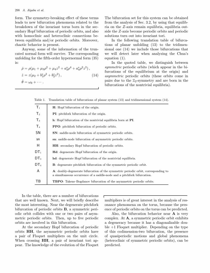
In the following translation table of bifurca-tions of planar unfolding (13) to the tridimen-sional one (14) we include those bifurcations thatwe will detect later when analyzing the Chua’sequation (1).

In the quoted table, we distinguish betweensymmetric periodic orbits (which appear in the bi-furcations of the equilibrium at the origin) andasymmetric periodic orbits (these orbits come inpairs due to the Z2-symmetry and are born in thebifurcations of the nontrivial equilibria).

Table 1. Translation table of bifurcations of planar system (13) and tridimensional system (14).

T1 H: Hopf bifurcation of the origin.

T2 PI: pitchfork bifurcation of the origin.

T3 h: Hopf bifurcation of the nontrivial equilibria born at PI.

T4 PPO: pitchfork bifurcation of periodic orbits.

SN SN: saddle-node bifurcation of symmetric periodic orbits.

sn sn: saddle-node bifurcation of asymmetric periodic orbits.

H HH: secondary Hopf bifurcation of periodic orbits.

DT1 Hd: degenerate Hopf bifurcation of the origin.

DT3 hd: degenerate Hopf bifurcation of the nontrivial equilibria.

DT4 B: degenerate pitchfork bifurcation of the symmetric periodic orbit.

A A: doubly-degenerate bifurcation of the symmetric periodic orbit, corresponding to

a simultaneous occurrence of a saddle-node and a pitchfork bifurcation.

TB TBPO: Takens–Bogdanov bifurcation of the asymmetric periodic orbits.

In the table, there are a number of bifurcationsthat are well known. Next, we will briefly describethe most interesting. Near the degenerate pitchforkbifurcation of periodic orbits B, a symmetric peri-odic orbit collides with one or two pairs of asym-metric periodic orbits. Then, up to five periodicorbits are involved in this bifurcation.

At the secondary Hopf bifurcation of periodicorbits HH, the asymmetric periodic orbits havea pair of Floquet multipliers on the unit circle.When crossing HH, a pair of invariant tori ap-pear. The knowledge of the evolution of the Floquet

multipliers is of great interest in the analysis of res-onance phenomena on the torus, because the pres-ence of periodic orbits on the torus can be predicted.

Also, the bifurcation behavior near A is verycomplex. At A, a symmetric periodic orbit exhibitsa degeneracy because it has a diagonalizable dou-ble +1 Floquet multiplier. Depending on the typeof this codimension-two bifurcation, the presenceof quasiperiodic motions and global phenomena(heteroclinic of symmetric periodic orbits), can bepredicted.


Finally, another important remark is relatedto the behavior near the Takens–Bogdanov bifur-cation of the asymmetric periodic orbits TBPO.Here, the asymmetric orbits have a nondiagonaliz-able double +1 Floquet multiplier, and one expectsthe presence of quasiperiodic motions and globalphenomena: homoclinic of asymmetric periodicorbits, . . .

A number of these phenomena will be put inevidence in the next section.

4. Numerical Study

At this point, we present some numerical work tocorroborate that the above-mentioned bifurcationseffectively appear in the Chua’s equation (1).

Generically, the behavior on the invariant toruswill be different when including the truncatedterms, due to phaselocking. Moreover, in thetruncated system, the torus breaks in a spheroidalsurface filled with orbits joining a nontrivial equi-librium point with a periodic orbit. This verydegenerate situation will disappear by addinghigher-order terms. Instead, we must expectcomplex heteroclinic structure and also homo-clinic behavior related to equilibria and periodicorbits, . . .

α

●

● ●

●● ●●

PD

DHP

●● ●

=-1.57

=-1.6

=-1.7

α

α

αTBPO

TBPOHH

HH HH

HHTBPO

TBPO

TBPO

,TBPO

HP

HP

HP

Fig. 3. Planar sections of the bifurcation set for the Chua’sequation (1) for different values of α, showing the differentshapes for the secondary Hopf bifurcation of periodic orbitsHH. We have also drawn the curve of Takens–Bogdanovbifurcations of periodic orbits TBPO that emerged from thedegenerate Hopf–pitchfork point DHP.

In our analysis, we will fix a = −1, γ = 0.3 > 0in Chua’s equation (1). Then, the degenerate Hopf–pitchfork bifurcation takes place at the criticalvalues cc ≈ 0.76923, βc = 0.09 and αc = −1.69.

0.04 0.05 0.06β

0.85

0.90

0.95

1.00

1.05

c

HH

HHA

TBPO’

PD

HP

TBPO’

0.0470 0.0475 0.0480β

0.990

0.992

0.994

0.996

c

PD

HH

TBPO’

PD

0.0527 0.0530 0.0533β

0.944

0.946

0.948

c

HH

HH2

PD

PD

PD2

PD2

PD4

PD4

HH4

TBPO’

TBPO2’

TBPO4’

Fig. 4. A partial bifurcation set for the Chua’s equation (1)with α = −1.57, γ = 0.3, a = −1, near the degenerate Hopf–pitchfork point. In the middle part, there is a zoom showingthe curves HH and PD. In the lower part, there is a zoomof the Takens–Bogdanov bifurcations of periodic orbits point,and the sequence of period-doubling bifurcations.


Fig. 5. A partial bifurcation set for the Chua’s equation (1)with α = −1.6, γ = 0.3, a = −1, near the degenerate Hopf–pitchfork point. In the lower part, there is a zoom of theHopf–pitchfork point.

We will take two slices α = constant of the tridi-mensional parameter space. The sections will betaken on both sides of the critical value αc. Namely,we will consider α = −1.7 and α = −1.6. Increas-ing α a bit more, the shape of the secondary Hopfbifurcation HH changes suddenly, because it inter-sects a period-doubling bifurcation PD, which doesnot arise from the local analysis of the planar sys-tem (see Fig. 3). We have included another sliceα = −1.57 to put this fact in evidence.

Notice that the secondary Hopf bifurcationof periodic orbits HH is present in three sec-tions. In the first situation α = −1.7, HH is not

Fig. 6. A partial bifurcation set for the Chua’s equation (1)with α = −1.6, γ = 0.3, a = −1, near the degenerate Hopf–pitchfork point. In the lower part, there is a zoom of theHopf–pitchfork point.

directly related to the Hopf–pitchfork bifurca-tion (of type Ib [Guckenheimer & Holmes, 1983,Sec. 7.5]). Then, we cannot detect HH in our localanalysis. In the second section α = −1.6, HH startsin a nondegenerate Hopf–pitchfork bifurcation (oftype VIa [Guckenheimer & Holmes, 1983, Sec. 7.5])and ends at a Takens–Bogdanov bifurcation of pe-riodic orbits TBPO, as obtained in our previoustheoretical analysis. Finally, for α = −1.57, thesecondary Hopf bifurcation of periodic orbits HHis broken into two branches when intersecting theperiod-doubling bifurcation PD. The intersectionpoints of HH and PD (labeled as TBPO′ in Figs. 3and 4) correspond also to Takens–Bogdanov bifur-cations of periodic orbits. Notice that the Takens–


-0.15 0.35

0.01

-0.05x

z

0.061 0.068-0.002

0.005

x

z

Fig. 7. Projection onto the xz plane of the torus attractorcorresponding to β = 0.0629, c = 0.9, α = −1.6, γ = 0.3,a = −1. The periodic orbit inside the torus is also shown. Inthe lower part, we include a Poincare section of the torus.

Bogdanov bifurcations of periodic orbits TBPOand TBPO′ are qualitatively different. The firstone corresponds to a nondiagonalizable double +1Floquet multiplier of a periodic orbit (strong 1:1resonance), whereas in TBPO′ there is a nondiag-onalizable double −1 Floquet multiplier (strong 1:2resonance).

This last is a very interesting situation,because one expects to find a Feigenbaum cas-cade of period-doubling bifurcations (which leadsto chaotic attractors), and consequently one alsoexpects to find a sequence of resonances 1:2, 1:4,1:8, . . . (see [Kuznetsov, 1995]). These facts can beviewed in the lower part of Fig. 4, where we havelabeled with PD2 and PD4 the two first period-doubling bifurcations of the sequence, and withHH2 and HH4 the curves where double-period andquadruple-period (respectively) tori emerge.

Anyway, our primary objective is to analyze indetail the sections α = −1.6, α = −1.7 (which aredirectly related with the degenerate Hopf–pitchforkbifurcation).

The bifurcation sets, for α = −1.6 and α =−1.7 are presented in Figs. 5 and 6, respectively.

0.05 0.06 0.07β

0

50

100

Arg

D

TBPO HP

Fig. 8. Evolution of the argument of the Floquet multiplier(in degrees) when moving on HH in the Chua’s equation (1)with α = −1.6, γ = 0.3, a = −1.

Notice that all the elements that appear have beenpreviously detected in the analytical study:

• The Hopf bifurcation of the origin H (green line),where a symmetric periodic orbit emerges.• The pitchfork bifurcation of the origin PI (red

line).• The Hopf bifurcation of the nontrivial equilibria

h (blue line), where a pair of asymmetric periodicorbits is born.• The pitchfork bifurcation of periodic orbits PPO

(yellow line), where the symmetric and the pairof asymmetric periodic orbits collapse.• The degenerate Hopf bifurcation of the origin

Hd.• The degenerate Hopf bifurcation of the nontrivial

equilibria hd.• The saddle-node bifurcation of symmetric peri-

odic orbits SN (orange line), starting from Hd.• The saddle-node bifurcation of asymmetric peri-

odic orbits sn (brown line), starting from hd.• The secondary Hopf bifurcation of periodic orbits

HH (black line).• The saddle-node–pitchfork bifurcation of periodic

orbits A.• The degenerate pitchfork bifurcation of periodic

orbits B.• The Takens–Bogdanov bifurcation of periodic

orbits TBPO.

In both figures, we have also included a zoomof the codimension-two Hopf–pitchfork points HP(of types VIa and Ib [Guckenheimer & Holmes,1983, Sec. 7.5], respectively) because several curvesare very close.


0.03 0.05 0.07β

0.8

0.9

1.0

1.1

c

HP

TBPO

HH

D

0.055 0.065β

0.87

0.94

c

1:4

1:5

1:6

1:7

1:8

HH

Fig. 9. A partial bifurcation set for the Chua’s equation (1)with α = −1.6, γ = 0.3, a = −1, showing the curve of sec-ondary Hopf bifurcations of periodic orbits and the curves ofsaddle-node bifurcations of periodic orbits corresponding toresonances 1:4, 1:5, 1:6, 1:7, 1:8. In the lower part, we showa zoom of point where the saddle-node curves intersect thesecondary Hopf bifurcation curve.

In the window of Fig. 5 there is a Takens–Bogdanov bifurcation of the origin TB, from whicha curve of heteroclinic connections Het emerges.This curve ends when it reaches the Hopf bifurca-tion of the nontrivial equilibria h, giving rise to aHopf-Shil’nikov bifurcation HS (see [Hirschberg &Knobloch, 1993]). The behavior is remarkable ofthe pitchfork bifurcation of periodic orbits PPOstarting from HP: it approaches TB and laterseparates.

In the following, we will look carefully at thezones where dynamical behavior related to thequasiperiodic motions (born in HH) takes place.We will assume on the rest that α = −1.6.

-0.7 0.0 0.7x

-0.04

0.00

0.04

z

0.0 0.5 1.0t

-0.04

0.00

0.04

z

Fig. 10. Projection onto the xz-plane of a periodic orbit inthe Chua’s equation (1) for parameter values β = 0.02604,c = 1.11779, α = −1.6, γ = 0.3, a = −1; inside the 1:5 reso-nance zone. In the lower part, we show a temporal profile ofthe periodic orbit along a normalized period.

In Fig. 7 we present a torus attractor (blue),corresponding to β = 0.0629, c = 0.9. The peri-odic orbit that gives rise to the torus is the red linedrawn inside. At the bottom of this figure, we alsoinclude a Poincare section, showing both the torusattractor and the periodic orbit.

It is well known that resonance phenomena onthe torus yields new bifurcation behaviors. Theperiodic orbit that undergoes the secondary Hopfbifurcation HH has a conjugate pair of Floquetmultiplier on the unit circle. In Fig. 8, we presentthe evolution of the argument of the Floquet multi-plier when moving along the curve HH. This will bevery important to predict resonance phenomena onHH, that occur when the Floquet multiplier movesthrough a root of the unity. Notice that the end-points of the curve HH are HP and TBPO. At


0.0600 0.0605 0.0610 0.0615β

0.91

0.92

0.93

cHH

TBPO4

HH4

PD4

PD16

PD8

HH8TBPO4’

sn4

sn4

Fig. 11. Zoom of the bifurcation set for the Chua’s equation(1) with α = −1.6, γ = 0.3, a = −1, near the 1:4 resonancepoint on HH. We show the secondary Hopf bifurcation of 4Tperiodic orbits HH4, the saddle-node bifurcation of periodicorbits sn4 corresponding to resonance 1:4, and the period-doubling sequence.

both points, the argument of the Floquet multiplieris zero, as pointed out in the figure.

As the argument is always less than 105◦, wecannot expect to find the 1:3 strong resonance, butthe 1:4 strong resonance will be present.

Note that the curve representing the argumentof the Floquet multiplier along HH has a parabola-like shape. There is a point (labeled D in Figs. 8and 9) where an angular degeneracy occurs (i.e. theargument fails to vary monotonically).

The implications of this angular degeneracy areconsidered by Peckham et al., [1995]. Then, inthose aspects related to weak resonance, we expectto find Arnold’s tongues with a particular shape(called by the authors as “banana” and “bananasplit”). The curves of saddle-node bifurcations ofperiodic orbits that bound the Arnold’s tongues in-tersect HH twice. In Fig. 9, we have drawn thesaddle-node bifurcations of periodic orbits corre-sponding to resonances 1:5, 1:6, 1:7, 1:8. Eachcurve of saddle-node bifurcations of these periodicorbits has three branches: one joining both tips,and two open branches, each starting from one tip.The different pairs of open branches have a com-mon asymptotic behavior: They are tangent to apair of curves related to homoclinic connections ofthe origin (not drawn in the figure). Similar be-haviors, but in the Hopf–saddle-node bifurcation,have been detected by Hirschberg and Laing [1995]and Kirk [1991]. Also, in the context of planar

0.064 0.069-0.003

0.003

x

z

-0.0070.0710.058

0.008

x

z

Fig. 12. Poincare section in the xz plane of the scenariocorresponding to resonance 1:4 in the Chua’s equation (1)with α = −1.6, γ = 0.3, a = −1. In the upper part(β = 0.0606909, c = 0.9235) we show the torus attractor,the repulsive periodic orbit (inside the torus) and two 4Tperiodic orbits, one attractive and the other saddle (outsidethe torus). In the lower part (β = 0.06092, c = 0.917), wecan see the principal periodic orbit (unstable), a 4T saddleperiodic orbit and a 4T stable periodic orbit surrounded bya 4T torus repellor.

diffeomorphisms, these phenomena have been putin evidence by Broer et al. [1998].

We also remark the behavior of the open branchstarting from the tip on the right, where theyexhibit a cusp-like behavior before they approachtangentially.

In Fig. 10 we have drawn a periodic orbit inthe Chua’s equation (1) for parameter values β =0.02604, c = 1.11779, inside the 1:5 resonance zone.This 5T periodic orbit is close to a five-pulse homo-clinic of the origin.

With respect to the strong resonance 1:4, it islimited by one curve of saddle-node bifurcations of4T periodic orbits sn4, that cross twice HH (seealso Fig. 9).

A detailed analysis of sn4, presented in Fig. 11,shows the presence of a Takens–Bogdanov point ofthe asymmetric periodic orbits TBPO4 (a degen-eracy corresponding to a nondiagonalizable dou-ble +1 Floquet multiplier). From such a point, a


0.91 0.95 0.99c

45

55

65

Period

0.047 0.053 0.059 0.065β

0.9

1.0

c

HH

sn4

Fig. 13. Bifurcation diagram (c versus period) for theChua’s equation (1) with parameter values β = 0.053, α =−1.6, γ = 0.3, a = −1 near the 1:4 resonance point on HH.The points marked on the closed line correspond to the curveof saddle-node bifurcations of periodic orbits sn4 that boundthe resonance zone. In the lower part, we include a bifur-cation set with the eight curves of saddle-node bifurcationsof 4T periodic orbits corresponding to resonance 1:4. Theseeight curves collapse in pairs in four cusp points.

secondary Hopf bifurcation of the 4T periodicorbits, HH4, emerges. HH4 ends when it meets aperiod-doubling curve PD4. The intersection pointis another Takens–Bogdanov bifurcation of periodicorbits TBPO′4 (nondiagonalizable double −1 Flo-quet multiplier). This is the starting point of aFeigenbaum cascade. In Fig. 11, we have also drawnthe next steps in the sequence: HH8, PD8; HH16,PD16.

In Fig. 12 we present two Poincare sections,corresponding to parameter values inside the 1:4Arnold’s tongue. The upper Poincare section cor-responds to β = 0.0606909, c = 0.9235, whichin Fig. 11 is located near the tip. Here, the un-

stable manifold of the 4T saddle periodic orbit(represented by four green points) join the 4Tstable periodic orbit (represented by four bluepoints) and the torus attractor.

In the lower Poincare section we have selectedβ = 0.06092, c = 0.917. In the bifurcation set ofFig. 11, this point is located above and close toHH4. Now, the invariant torus is no longer present,and the stable manifold of the 4T saddle periodicorbit connects the unstable principal periodic orbitand the 4T torus repellor (represented by four redclosed lines).

These behaviors have been found to be in con-cordance with the type D2, following the classifica-tion of Chow et al. [1994], Sec. 4.4, in the analysis ofplanar systems with a double-zero eigenvalue, whichare invariant under a rotation of angle π/2.

Also, we remark that, on sn4, there is anotherTakens–Bogdanov bifurcation of periodic orbits atβ ≈ 0.05347, c ≈ 0.98024, but this point is outsidethe window of Fig. 11.

Finally, in order to put in evidence the complex-ity of the frontier of the 1:4 resonance zone, we haveincluded a bifurcation diagram (c versus period) forthe parameter values β = 0.053, α = −1.6, γ = 0.3,a = −1 (see Fig. 13).

The bifurcation diagram, represented in theupper part of Fig. 13, consists in a closed line(isola). We have marked two points, that corre-spond to the curve of saddle-node bifurcations ofperiodic orbits sn4 (blue line). Moreover, anothereight saddle-node bifurcations of 4T periodic orbitsare detected. These saddle-node bifurcations areorganized around four cusps. This kind of behav-ior has been observed by Broer et al. [1998] inthe analysis of the fattened Arnold family. It isalso remarkable that one of these new saddle-nodebifurcations of 4T periodic orbits crosses sn4.

Acknowledgments

This work was partially supported by the Con-sejerıa de Educacion y Ciencia de la Junta deAndalucıa.

ReferencesAlgaba, A., Freire, E. & Gamero, E. [1998] “Hypernor-

mal form for the Hopf-zero bifurcation,” Int. J. Bifur-cation and Chaos 8(10), 1857–1887.

Algaba, A., Freire, E., Gamero, E. & Rodrıguez-Luis,A. J. [1999a] “On a codimension-three unfoldingof the interaction of degenerate Hopf and pitchfork


bifurcations,” Int. J. Bifurcation and Chaos 9(7),1333–1362.

Algaba, A., Freire, E., Gamero, E. & Rodrıguez-Luis,A. J. [1999b] “A tame degenerate Hopf-pitchforkbifurcation in a modified van der Pol–Duffing oscil-lator,” Nonlin. Dyn., accepted.

Algaba, A., Freire, E., Gamero, E. & Rodrıguez-Luis, A.J. [1999c] “A three-parameter study of a degeneratecase of the Hopf-pitchfork bifurcation,” Nonlinearity12, 1177–1206.

Andronov, A., Leontovich, E., Gordon, I. & Maier, A.[1970] Qualitative Theory of Second Order DynamicsSystems (John Wiley, NY).

Broer, H., Simo, C. & Tatjer, J. C. [1998] “Towardsglobal models near homoclinic tangencies of dissipa-tive diffeomorphisms,” Nonlinearity 11, 667–770.

Chow, S. N., Li, C. & Wang, D. [1994] Normal Formsand Bifurcation of Planar Vector Fields (CambridgeUniversity Press).

Dumortier, F. [1991] “Local study of planar vector fields:Singularities and their unfolding,” in Structures in Dy-namics, Studies in Math. Physics, Vol. 2, eds. Broer,H. W., Dumortier, F., van Strien, S. J. & Takens, F.(North Holland, Amsterdam), pp. 161–242.

Guckenheimer, J. & Holmes, P. J. [1983] NonlinearOscillations, Dynamical Systems, and Bifurcations ofVector Fields (Springer, Berlin).

Hirschberg, P. & Knobloch, E. [1993] “Silnikov–Hopfbifurcation,” Physica D62, 202–216.

Hirschberg, P. & Laing, C. [1995] “Successive homoclinictangencies to a limit cycle,” Physica D89, 1–14.

Kirk, V. [1991] “Breaking of symmetry in the saddle-node Hopf bifurcation,” Phys. Lett. A154(5&6),243–248.

Krauskopf, B. & Rousseau, C. [1997] “Codimension-three unfoldings of reflectionally symmetric planarvector fields,” Nonlinearity 10(5), 1115–1150.

Kuznetsov, Yu. A. [1995] Elements of Applied Bifurca-tion Theory (Springer, NY).

Peckham, B. B., Frouzakis, C. E. & Kevrekidis, I. G.[1995] “Bananas and banana splits: A parametricdegeneracy in the Hopf bifurcation for maps,” SIAMJ. Math. Anal. 26(1), 190–217.

Pivka, L., Wu, C. W. & Huang, A. [1996] “Lorenz equa-tion and Chua’s equation,” Int. J. Bifurcation andChaos 6(12B), 2443–2489.

Documents

ON THE HOPF PITCHFORK BIFURCATION IN THE …chua/papers/Algaba00.pdf · International Journal of Bifurcation and Chaos, Vol. 10, No. 2 (2000) 291{305 c World Scienti c Publishing