The Non-Smooth Pitchfork Bifurcation: A Renormalization Analysis

L N C Adamson∗and A H Osbaldestin†

Department of MathematicsUniversity of Portsmouth

PortsmouthPO1 3HF, UK

January 7, 2015

Abstract

We give a renormalization group analysis of a system exhibiting a non-smooth pitchfork bifurcation to astrange non-chaotic attractor. For parameter choices satisfying two specified conditions, self-similar behaviourof the attractor on and near the bifurcation curve can be observed, which corresponds to a periodic orbit of anunderlying renormalization operator. We examine the scaling properties for various parameter choices includingthe so-called Pitchfork Critical Point. Finally, we study the autocorrelation function for the system and showthat it is equivalent to that present in symmetric barrier billiards.

1 Introduction

Strange non-chaotic attractors (SNAs) have been the focus of a broad wave a research into quasiperiodically forcedsystems over the past three decades. This began when Grebogi et al. (GOPY) gave an analytical proof of theirexistence in [8]. These objects are seemingly paradoxical in nature; in essence we have an attracting set whichis not finite and which is nowhere differentiable (fractal in fact), and yet nearby orbits on it do not diverge atan exponential rate over time. Indeed, prior to their discovery the terms ‘strange’ and ‘chaotic’ were used likesynonyms.

These pioneering authors then extended their work into to the evolution of these attractors in [3], where for ageneralised circle map the transition between quasiperiodic, strange non-chaotic and chaotic behaviour was studied.For the map under study there were three regions in two-dimensional parameter space which gave rise to thesebehaviours. It was shown that the set in parameter space for which the system exhibits SNAs has Cantor set-likestructure and lies between two boundary curves separating the other two behaviours, thus making it an intermediatebetween quasi-periodic and chaotic motion. In [16] it is shown that these attractors occur on a set of positivemeasure, thus making them physically important.

Further work on the characterisation of SNAs was presented in [15]. This gave a number of conditions which enableone to determine whether the attracting set is strange, which is highly useful as this is often difficult to determineanalytically.

Of interest to us in this paper is the model studied by Glendinning in [7], in which the non-smooth pitchforkbifurcation for SNAs is studied. The results of this paper will be summarised for a qualitatively equivalent model in

∗luke.adamson@port.ac.uk†andrew.osbaldestin@port.ac.uk

1

Section 2. The aim of this paper is to provide a renormalization group approach along the entire curve in parameterspace on which this bifurcation occurs.

Furthermore, in [10] a renormalization group approach was developed to study a route to SNA labelled the “blowoutbirth”. In fact, this is just the non-smooth pitchfork bifurcation studied by Glendinning but for a particular choiceof parameter. In [10] Kuznetsov et al. demonstrated that for a model qualitatively similar to that studied in [8],there are local scaling properties for certain choices of initial phase at the critical point in parameter space whichseparates a trivial attractor from SNAs. Furthermore, it is demonstrated that these scaling properties can be usedto examine the size and structure of the SNA near the critical point, demonstrating the self-similar structures whichoccur on smaller and smaller scales, and thus giving a full understanding of this bifurcation.

Work into the correlations and spectra of SNAs has been presented in [14], showing that they exhibit unusualproperties. The autocorrelation function (ACF) is self-similar with peaks occurring at resonant frequencies withrespect to the forcing, and the spectrum is a fractal curve on the complex plane. A renormalization approach wasdeveloped to study the ACF of the GOPY model in [6]. Numerically it was observed in [6] that the self-similaritycould be understood in terms of a period six orbit of a renormalization operator.

This topic was then rigorously examined in [11], showing that the autocorrelation function has peaks of magnitude1 − 1/

√5 ' 0.55 . . . at every third Fibonacci number for the golden mean forcing frequency, putting on firmer

footing earlier numerical results in [14] and [6]. This will be extended for the model under study in this paper inSection 4.

We begin with a review of the features of Glendinning’s model [7], but for which we consider a different, butqualitatively equivalent variant. In Section 3 we develop the renormalization group approach similar to that in[10] and explain the similarity between this and the more general approach seen for similar models (a thoroughsummary can be seen in [5]). We give necessary conditions on parameters, scaling factors and initial phases forperiodic behaviour of the renormalization operator to occur, in addition to explicit construction of these periodicorbits using a method of numerical approximation based on analysis of the growth rate of the attractor. Finally inSection 4 we provide a link between the ACF of the system under study and the ACF which appears in the studyof work we have previously conducted on symmetric barrier billiards [13].

2 The map and previous work

The map of interest to us in this paper is a generalisation of the map studied in [10] for which a renormalizationgroup approach was used to give an analysis of the birth of an SNA. It is given by

xi+1 = f(θi, xi) = 2σ(φ+ cos(2πθi))xi

(1 + x2i )1/2︸ ︷︷ ︸

∗

, (2.1)

θi+1 = θi + ω (mod 1). (2.2)

For simplicity in the renormalization analysis, we take ω to be the inverse of the golden mean throughout i.e.ω = (

√5 − 1)/2, although generalization to a broader class of quadratic irrationals is possible [1]. The non-

linear function * highlighted in (2.1) is qualitatively equivalent to tanh(x), and in [7] this system was studiedby Glendinning for the latter choice. The reason for the change to form * is the same as it was in [10] wherethe same model (with cos replaced by sin) was studied for the case of φ = 0; composition of functions in thisclass yield another function in this class, which means that in the renormalization analysis the x variable atcharacteristic times will also be a member of this class. In particular if f1,2(x) = A1,2x(1 + B1,2x

2)−1/2 thenf1(f2(x)) = A1A2x(1 + (B2 +B1A

22)x2))−1/2.

Due to the qualitative similarity of the system (2.1)−(2.2) to that studied by Glendinning, the arguments in [7] canbe carried over directly and will now be summarised.

2

0 0.5 1 1.5 20

0.2

0.4

0.6

0.8

1

1.2

1.4

1.6

1.8

2

φ

σ

Region 1

Region 2

Region 3

B

C

A

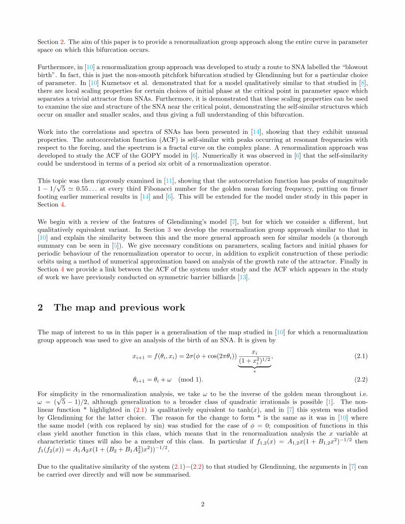
Figure 1: Plot of the first quadrant of the parameter plane (φ, σ) showing the three regions in which differentdynamical regimes occur and the bifurcation curves A,B and C which separate them.

The circle in phase space defined byL = {(θ, x)|x = 0}, (2.3)

is invariant under the map, and the stability of this set can be determined by calculation of its transverse Lyapunovexponent. Using the ergodicity in θ we can write this exponent as

λ =

∫ 1

0

ln∣∣∣∂f∂x

∣∣∣x=0

dθ, (2.4)

=1

2

∫ 1

0

ln(2σ(φ+ cos(2πθ)))2 dθ. (2.5)

In [7] it is shown that this integral is given by

λ =

{lnσ, 0 ≤ φ ≤ 1,

lnσ + ln(φ+√φ2 − 1), φ > 1.

(2.6)

As shown in Figure 1, (2.6) defines two bifurcation curves A and B on which the Lyapunov exponent for L is zero.In particular these curves are given by

A = {(φ, σ) |σ = 1, 0 ≤ φ ≤ 1}, (2.7)

B = {(φ, σ) |σ = (φ+√φ2 − 1)−1, φ > 1}. (2.8)

The circle L is thus stable for parameter choices below the union of these curves, and unstable above them.However, one more bifurcation takes place, as the system (2.1)−(2.2) becomes invertible for φ > 1. The behaviourbelow the union of curves A and B (Region 1 in Figure 1) is trivial as the attractor is simply L as shown in [9].Hence we define a third bifurcation curve as

C = {(φ, σ) |φ = 1, σ ≥ 1}. (2.9)

We now focus on the dynamics in Regions 2 and 3 shown in Figure 1. For choices of parameter in Region 2 it isshown in [7] (following the approach in [8]) that the system gives rise to a strange non-chaotic attractor (SNA). Inthis region the set L is unstable and because φ < 1 there are values θ̃ such that φ+ cos(2πθ̃) = 0. Now, as x = 0 isinvariant we conclude that the set of points (θ̃+ nω, 0) are all members of the attracting set for n ∈ N. Thus thereis a dense set of points on the θ axis such that x = 0. However as L is unstable it is not the attractor and so thereare non-zero values of x. This leads to a pinching effect indicating that the resulting attractor is not differentiableat any point and is thus strange.

3

To prove that the attractor is non-chaotic for any choice of parameter not on one of the bifurcation curves A andB, we use the approach shown in [8] to prove that the Lyapunov exponent is non-positive. Firstly we note that

d

dx

(x√

1 + x2

)≤ 1√

1 + x2, (2.10)

with equality only being true at x = 0. Inside Region 1 the attractor is L, so by our calculation of the transverseLyapunov exponent for L above we conclude that the exponent is negative for any parameter choice inside Region1. In Regions 2 and 3 x does not tend to zero and so the inequality is again strict. Hence∣∣∣∂f

∂x

∣∣∣xi,θi

<∣∣∣xi+1

xi

∣∣∣, (2.11)

and so from the definition of the Lyapunov exponent we have

λ = limN→∞

(1

N

N∑i=1

ln∣∣∣∂f∂x

∣∣∣xi,θi

)≤ limN→∞

(1

N

N∑i=1

ln∣∣∣xi+1

xi

∣∣∣) = limN→∞

(1

N

N∑i=1

ln |xi+1| − ln |xi|)

= 0. (2.12)

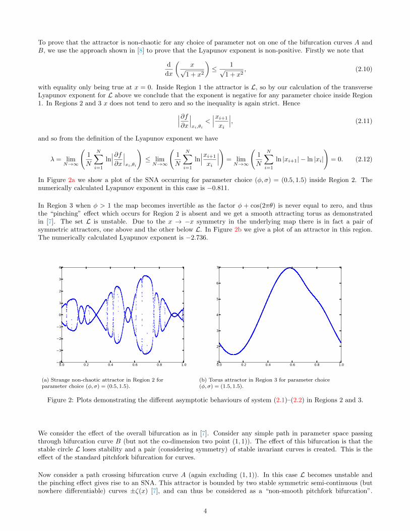
In Figure 2a we show a plot of the SNA occurring for parameter choice (φ, σ) = (0.5, 1.5) inside Region 2. Thenumerically calculated Lyapunov exponent in this case is −0.811.

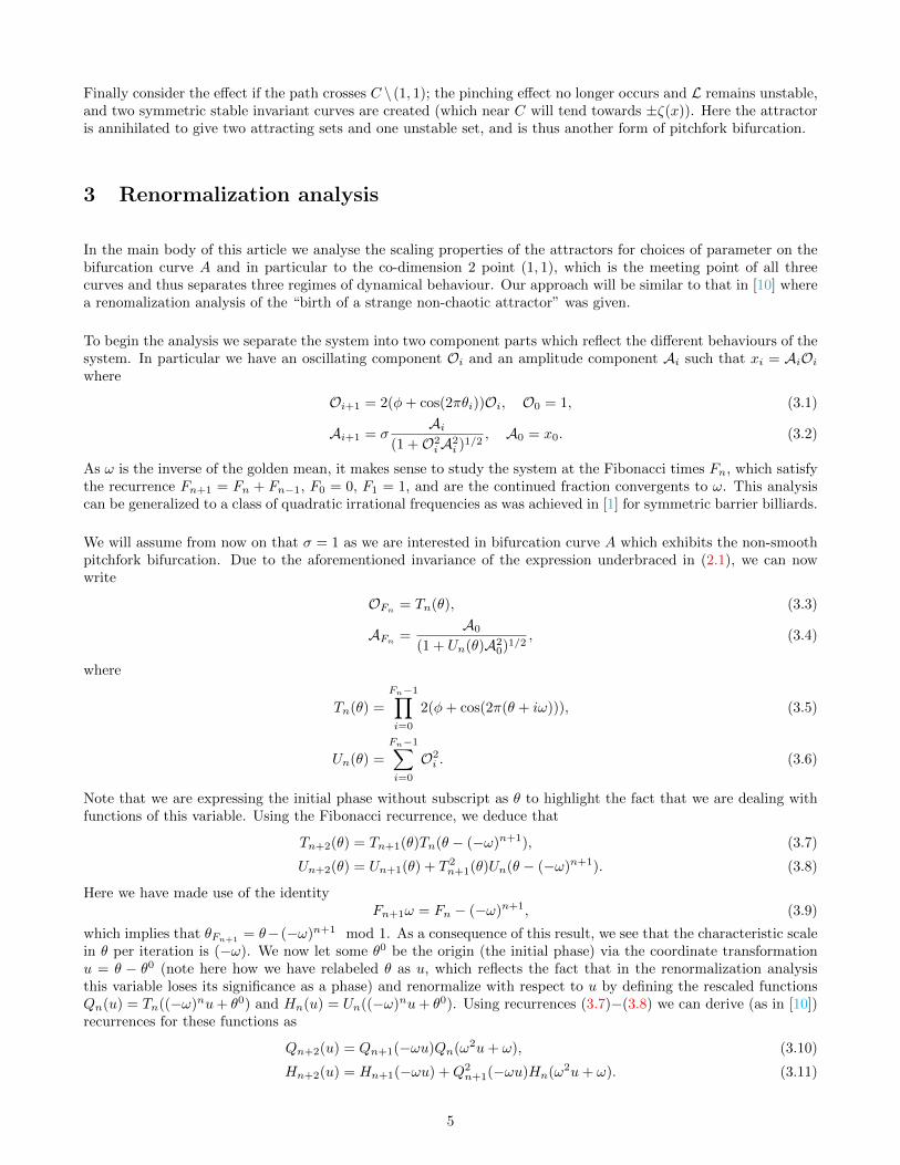
In Region 3 when φ > 1 the map becomes invertible as the factor φ + cos(2πθ) is never equal to zero, and thusthe “pinching” effect which occurs for Region 2 is absent and we get a smooth attracting torus as demonstratedin [7]. The set L is unstable. Due to the x → −x symmetry in the underlying map there is in fact a pair ofsymmetric attractors, one above and the other below L. In Figure 2b we give a plot of an attractor in this region.The numerically calculated Lyapunov exponent is −2.736.

0.0 0.2 0.4 0.6 0.8 1.0−4

−3

−2

−1

0

1

2

3

4

(a) Strange non-chaotic attractor in Region 2 forparameter choice (φ, σ) = (0.5, 1.5).

0.0 0.2 0.4 0.6 0.8 1.01

2

3

4

5

6

7

(b) Torus attractor in Region 3 for parameter choice(φ, σ) = (1.5, 1.5).

Figure 2: Plots demonstrating the different asymptotic behaviours of system (2.1)–(2.2) in Regions 2 and 3.

We consider the effect of the overall bifurcation as in [7]. Consider any simple path in parameter space passingthrough bifurcation curve B (but not the co-dimension two point (1, 1)). The effect of this bifurcation is that thestable circle L loses stability and a pair (considering symmetry) of stable invariant curves is created. This is theeffect of the standard pitchfork bifurcation for curves.

Now consider a path crossing bifurcation curve A (again excluding (1, 1)). In this case L becomes unstable andthe pinching effect gives rise to an SNA. This attractor is bounded by two stable symmetric semi-continuous (butnowhere differentiable) curves ±ζ(x) [7], and can thus be considered as a “non-smooth pitchfork bifurcation”.

4

Finally consider the effect if the path crosses C \ (1, 1); the pinching effect no longer occurs and L remains unstable,and two symmetric stable invariant curves are created (which near C will tend towards ±ζ(x)). Here the attractoris annihilated to give two attracting sets and one unstable set, and is thus another form of pitchfork bifurcation.

3 Renormalization analysis

In the main body of this article we analyse the scaling properties of the attractors for choices of parameter on thebifurcation curve A and in particular to the co-dimension 2 point (1, 1), which is the meeting point of all threecurves and thus separates three regimes of dynamical behaviour. Our approach will be similar to that in [10] wherea renomalization analysis of the “birth of a strange non-chaotic attractor” was given.

To begin the analysis we separate the system into two component parts which reflect the different behaviours of thesystem. In particular we have an oscillating component Oi and an amplitude component Ai such that xi = AiOiwhere

Oi+1 = 2(φ+ cos(2πθi))Oi, O0 = 1, (3.1)

Ai+1 = σAi

(1 +O2iA2

i )1/2

, A0 = x0. (3.2)

As ω is the inverse of the golden mean, it makes sense to study the system at the Fibonacci times Fn, which satisfythe recurrence Fn+1 = Fn + Fn−1, F0 = 0, F1 = 1, and are the continued fraction convergents to ω. This analysiscan be generalized to a class of quadratic irrational frequencies as was achieved in [1] for symmetric barrier billiards.

We will assume from now on that σ = 1 as we are interested in bifurcation curve A which exhibits the non-smoothpitchfork bifurcation. Due to the aforementioned invariance of the expression underbraced in (2.1), we can nowwrite

OFn= Tn(θ), (3.3)

AFn=

A0

(1 + Un(θ)A20)1/2

, (3.4)

where

Tn(θ) =

Fn−1∏i=0

2(φ+ cos(2π(θ + iω))), (3.5)

Un(θ) =

Fn−1∑i=0

O2i . (3.6)

Note that we are expressing the initial phase without subscript as θ to highlight the fact that we are dealing withfunctions of this variable. Using the Fibonacci recurrence, we deduce that

Tn+2(θ) = Tn+1(θ)Tn(θ − (−ω)n+1), (3.7)

Un+2(θ) = Un+1(θ) + T 2n+1(θ)Un(θ − (−ω)n+1). (3.8)

Here we have made use of the identityFn+1ω = Fn − (−ω)n+1, (3.9)

which implies that θFn+1= θ−(−ω)n+1 mod 1. As a consequence of this result, we see that the characteristic scale

in θ per iteration is (−ω). We now let some θ0 be the origin (the initial phase) via the coordinate transformationu = θ − θ0 (note here how we have relabeled θ as u, which reflects the fact that in the renormalization analysisthis variable loses its significance as a phase) and renormalize with respect to u by defining the rescaled functionsQn(u) = Tn((−ω)nu+ θ0) and Hn(u) = Un((−ω)nu+ θ0). Using recurrences (3.7)−(3.8) we can derive (as in [10])recurrences for these functions as

Qn+2(u) = Qn+1(−ωu)Qn(ω2u+ ω), (3.10)

Hn+2(u) = Hn+1(−ωu) +Q2n+1(−ωu)Hn(ω2u+ ω). (3.11)

5

The initial conditions for these recurrences are Q0 = 1, Q1(u) = T1(θ0−ωu) = 2(φ+cos(2π(θ0−ωu))) and H0 = 0,H1 = 1. Note that this corrects an error in [10], where the change in coordinates was not implemented correctlyinto the definition of Qn and Hn. This did not affect the numerical results in that paper, but we have found thatit leads to incorrect scaling factors for certain choices of the initial phase.

This system was studied previously for the case φ = 0 in [10] for the study of the “birth of an SNA”. In [10] it isshown that for certain choices of initial phase, iteration of (3.10) leads to periodic behaviour of Qn. Due to theresults of previous work in [11] (for example), we conclude that a necessary condition for periodicity is that thezeros of the initial condition Q1 lie in Q(ω), the field of rationals over ω.

In this case we see that (3.11) is a periodically driven linear recurrence (although the linearity is deceptive!).Assuming the period of Q2

n is p, we expect it to produce a factor of growth over a period i.e. Hn+p(u) ' ν2Hn(u).Due to the fact that Un describes the growth of the attractor, and due to the form of (3.2), we conclude thatthe amplitude of the attractor decreases by a factor of ν over a period. This approach enables us to see how theconstituent parts of the underlying system behave at smaller and smaller scales.

We remark that in keeping with approaches used elsewhere (for extensive examples see [5]) we could have formulatedthis problem slightly differently. In particular we define the functions fn(x, θ) by the equation

xi+Fn = fn(xi, θi). (3.12)

The apparent similarity between these two methods is seen as we can now write

fn(x, θ) =Tn(θ)x√

1 + Un(θ)x2. (3.13)

Indeed, up until this point both approaches are identical. Once again we define a new coordinate system u = θ− θ0and we now renormalize by changing the scales of x and u by defining the rescaled functions

gn(x, u) = αnfn(x/αn, (−ω)nu+ θ0). (3.14)

The scale in u is the same as before (for θ) but the new variable α represents the change in scale for x per step ofthe renormalization. By manipulating (3.14) the renornalization operator can be shown to be given by

gn+2(x, u) = α2gn(α−1gn+1(x/α,−uω + (−ω)−(n+1)θ0), ω2u+ ω + (−ω)−nθ0). (3.15)

For the model under study, direct substitution yields

gn(x, u) =Qn(u)x√

1 + H̃n(u)x2, (3.16)

where H̃n(u) = α−2nHn(u), and Qn, Hn are as defined in (3.10)−(3.11). Hence the difference is in the scaling ofHn. This is a correction of the previous approach in [5], and we will now clarify the relationship between the tworenormalization schemes. Indeed, we can now pick α to ensure periodicity (with period p) of H̃. Asymptoticallywe have

α2(n+p)H̃n+p(u) = Hn+p(u) = ν2Hn(u) = ν2α2nH̃n(u). (3.17)

Thus for periodicity we require α = ν1/p.

We will now determine conditions on φ and θ0 necessary for periodic behaviour to occur. In particular, the zerosof Q1 are given by

x = ω−1(±cos−1(−φ)

2π+ θ0 + n

), n ∈ Z. (3.18)

The conditions for these points to be in Q(ω) are clearly that θ0 + cos−1(−φ)/2π ∈ Q(ω) and θ0− cos−1(−φ)/2π ∈Q(ω) (note that ω−1 = 1 + ω). Hence we require that both θ0 and cos−1(−φ)/π are in Q(ω).

For each value of φ satisfying this constraint, we can pick any θ0 ∈ Q(ω) as an origin, and we expect that eachchoice will give different local scaling properties due to the multi-fractal nature of the SNA [6]. The case φ = 0 was

6

15 20 25 30 35 40 45 50 55 600

0.05

0.1

0.15

0.2

0.25

0.3

0.35

0.4

0.45

Sn

n

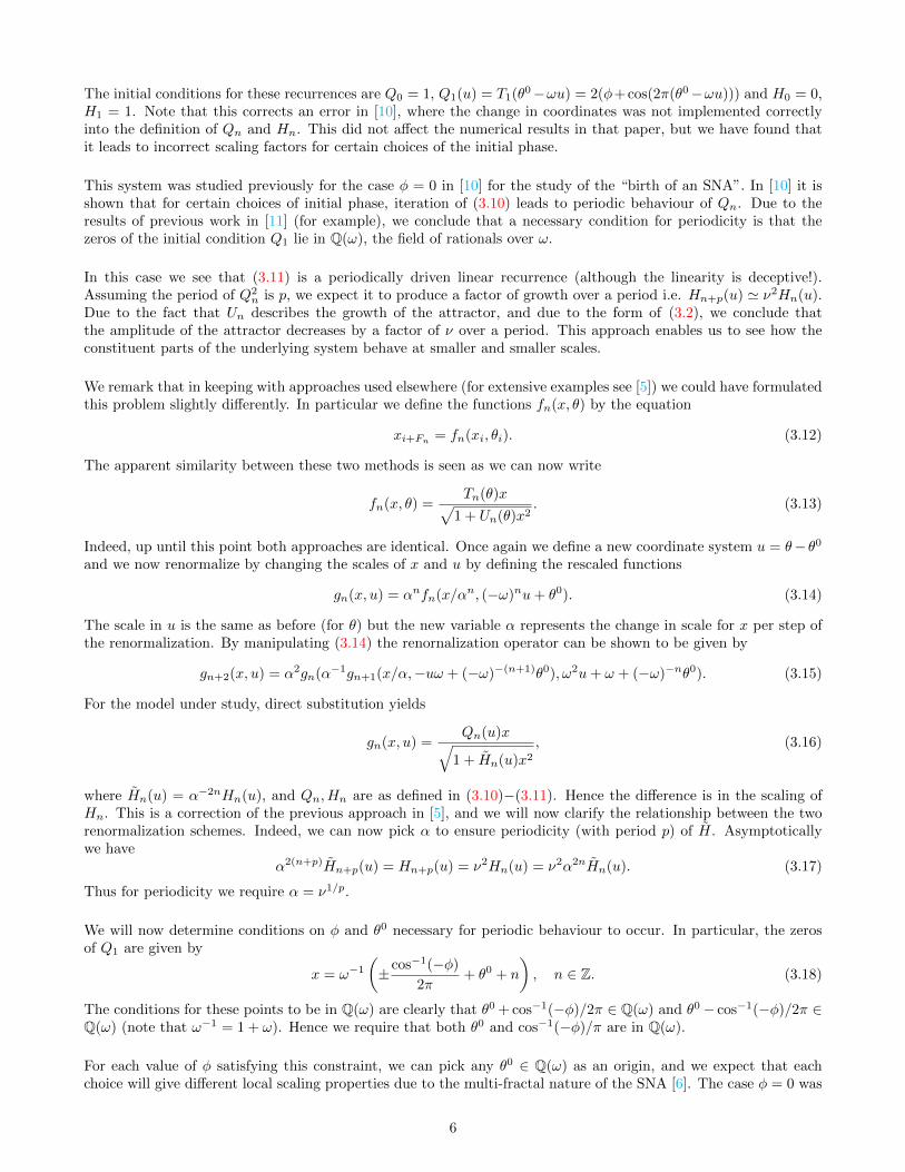
Figure 3: Plot of the standard deviation Sn of γn at time index n for n = 19, . . . , 57 (φ = 0.5, θ0 = 0).

studied extensively in [10] for several initial phases θ0 in Q(ω), each of which resulted in periodic behaviour of therenormalization operator as our theory predicts. We will now illustrate the material derived thus far in this sectionby examining the case of φ = 0.5. In this case cos−1(−φ)/π = 2/3 and so with a choice of θ0 in Q(ω) we expectperiodicity of (3.10) and therefore a scaling law in a vicinity of θ0.

We take θ0 = 0, and represent the resulting Q1 by a polynomial interpolant accurate to machine precision. This isachieved using the Chebfun system, an incredibly useful extension developed for Matlab. See (for example) [4] formore details. Iterating forward we calculate that Q2

n converges to a period four orbit. Due to the chaotic natureof the inverse of the iterated function system given by the contractions φ1(x) = −ωx and φ2(x) = ω2x+ ω, after afinite number of iterations this periodicity is no longer observable as the system degenerates to noise. Thus we havea finite range of iterates for which the initial transient behaviour has disappeared and in which the system has notdegenerated to noise, leaving us with the periodic orbit we desire.

We can estimate ν by looking at the periodic growth functions given by

γn(u) =Hn+p(u)

Hn(u). (3.19)

From (3.17) we expect that asymptotically γn → ν2 as n → ∞ (p = 4). By substituting the periodic solution of(3.10) into (3.11) we examine the standard deviation of γn(u), Sn. Due to the previous argument with regard to the(numerical) evolution of Qn, there will be transient behaviour followed by periodicity which will then degenerate tonoise. Hence a plot of Sn against n will produce a “U-shaped” curve; the flat region is indicative of convergence tothe desired periodic orbit, whereas the left and right sides correspond to transients and noise respectively. This isshown in Figure 3 for the case under study. We choose the n which minimises the standard deviation, and thus theγn which is the “most constant”. Then we calculate the mean value of γn and take the square root of it to obtainν.

We have checked the proposed method of estimating ν by comparing the factors to those obtained in [10] for φ = 0with cos replaced by sin in (2.1). For example in the case θ0 = 0.25 we find the scaling factor to four decimal placesto be ν = 7.4246, in perfect agreement with [10].

Returning to the problem under study (φ = 0.5, θ0 = 0), we find n = 37 to give a minimum standard deviation of' 7 × 10−5, and by calculating the mean value of γ37 we estimate the value of ν to be ν = 4.127 (to 3 d.p). Thisgives us the scaling factor for x as α = ν1/4 = 1.425 (again to 3 d.p).

Note that Qn is actually periodic with period eight, but due to a symmetry in the solutions the period of Q2n is four.

We can now substitute these solutions into (3.16) and plot the period eight orbit of the renormalization operatorgn(x, u) as shown in Figure 4.

Hence the evolution of the system at time Fk is the same after appropriate scaling as the system at time F8m+k.In fact however, due to the aforementioned symmetry which can also seen in Figure 4, the system actually displayssimilar behaviour every four steps of the renormalization operator as the model under study is symmetric. Inparticular, this means that the dynamics with some starting point (x, u) is the same as the dynamics starting from

7

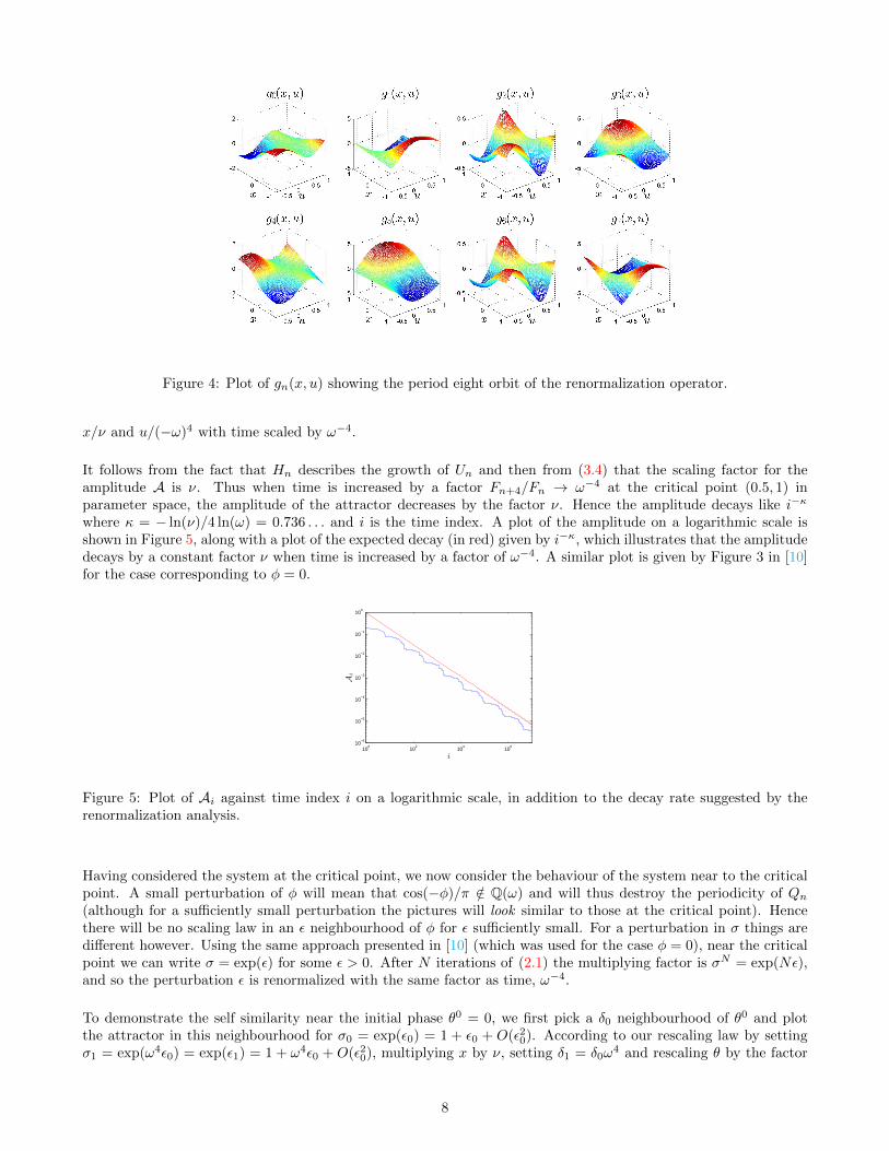
Figure 4: Plot of gn(x, u) showing the period eight orbit of the renormalization operator.

x/ν and u/(−ω)4 with time scaled by ω−4.

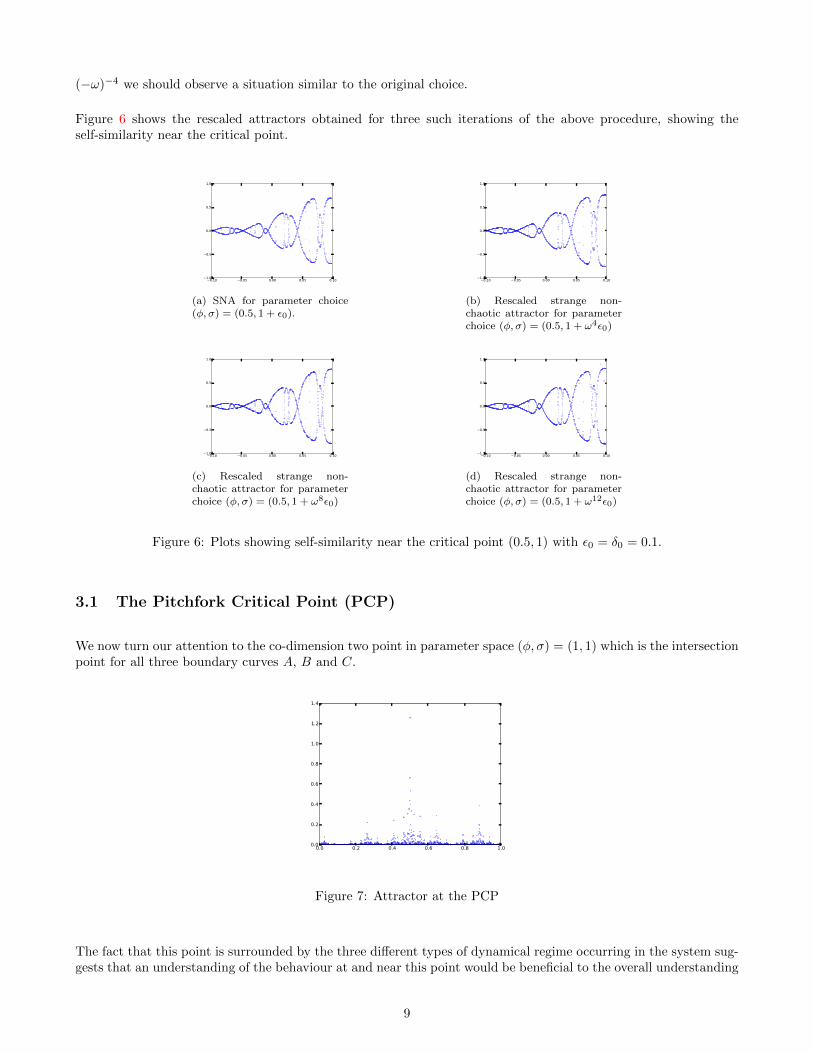
It follows from the fact that Hn describes the growth of Un and then from (3.4) that the scaling factor for theamplitude A is ν. Thus when time is increased by a factor Fn+4/Fn → ω−4 at the critical point (0.5, 1) inparameter space, the amplitude of the attractor decreases by the factor ν. Hence the amplitude decays like i−κ

where κ = − ln(ν)/4 ln(ω) = 0.736 . . . and i is the time index. A plot of the amplitude on a logarithmic scale isshown in Figure 5, along with a plot of the expected decay (in red) given by i−κ, which illustrates that the amplitudedecays by a constant factor ν when time is increased by a factor of ω−4. A similar plot is given by Figure 3 in [10]for the case corresponding to φ = 0.

100

102

104

106

10−6

10−5

10−4

10−3

10−2

10−1

100

i

Ai

Figure 5: Plot of Ai against time index i on a logarithmic scale, in addition to the decay rate suggested by therenormalization analysis.

Having considered the system at the critical point, we now consider the behaviour of the system near to the criticalpoint. A small perturbation of φ will mean that cos(−φ)/π /∈ Q(ω) and will thus destroy the periodicity of Qn(although for a sufficiently small perturbation the pictures will look similar to those at the critical point). Hencethere will be no scaling law in an ε neighbourhood of φ for ε sufficiently small. For a perturbation in σ things aredifferent however. Using the same approach presented in [10] (which was used for the case φ = 0), near the criticalpoint we can write σ = exp(ε) for some ε > 0. After N iterations of (2.1) the multiplying factor is σN = exp(Nε),and so the perturbation ε is renormalized with the same factor as time, ω−4.

To demonstrate the self similarity near the initial phase θ0 = 0, we first pick a δ0 neighbourhood of θ0 and plotthe attractor in this neighbourhood for σ0 = exp(ε0) = 1 + ε0 + O(ε20). According to our rescaling law by settingσ1 = exp(ω4ε0) = exp(ε1) = 1 + ω4ε0 + O(ε20), multiplying x by ν, setting δ1 = δ0ω

4 and rescaling θ by the factor

8

(−ω)−4 we should observe a situation similar to the original choice.

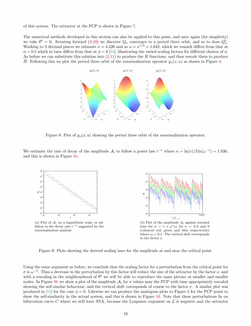
Figure 6 shows the rescaled attractors obtained for three such iterations of the above procedure, showing theself-similarity near the critical point.

−0.10 −0.05 0.00 0.05 0.10−1.0

−0.5

0.0

0.5

1.0

(a) SNA for parameter choice(φ, σ) = (0.5, 1 + ε0).

−0.10 −0.05 0.00 0.05 0.10−1.0

−0.5

0.0

0.5

1.0

(b) Rescaled strange non-chaotic attractor for parameterchoice (φ, σ) = (0.5, 1 + ω4ε0)

−0.10 −0.05 0.00 0.05 0.10−1.0

−0.5

0.0

0.5

1.0

(c) Rescaled strange non-chaotic attractor for parameterchoice (φ, σ) = (0.5, 1 + ω8ε0)

−0.10 −0.05 0.00 0.05 0.10−1.0

−0.5

0.0

0.5

1.0

(d) Rescaled strange non-chaotic attractor for parameterchoice (φ, σ) = (0.5, 1 + ω12ε0)

Figure 6: Plots showing self-similarity near the critical point (0.5, 1) with ε0 = δ0 = 0.1.

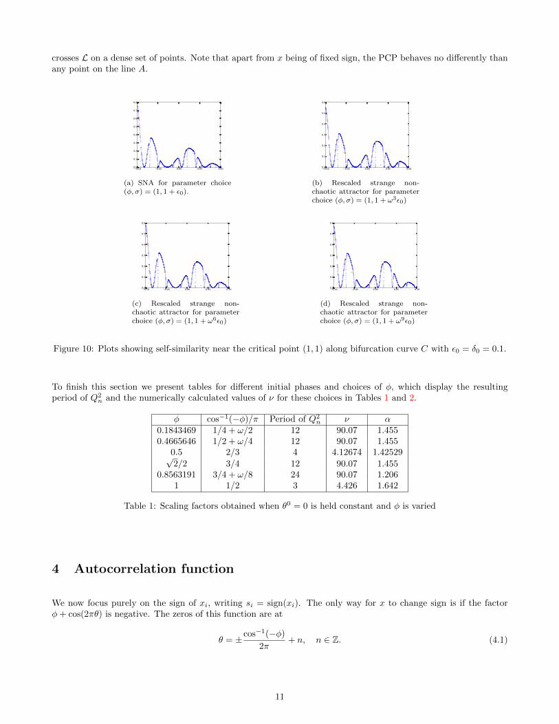
3.1 The Pitchfork Critical Point (PCP)

We now turn our attention to the co-dimension two point in parameter space (φ, σ) = (1, 1) which is the intersectionpoint for all three boundary curves A, B and C.

0.0 0.2 0.4 0.6 0.8 1.00.0

0.2

0.4

0.6

0.8

1.0

1.2

1.4

Figure 7: Attractor at the PCP

The fact that this point is surrounded by the three different types of dynamical regime occurring in the system sug-gests that an understanding of the behaviour at and near this point would be beneficial to the overall understanding

9

of this system. The attractor at the PCP is shown in Figure 7.

The numerical methods developed in this section can also be applied to this point, and once again (for simplicity)we take θ0 = 0. Iterating forward (3.10) we discover Qn converges to a period three orbit, and so to does Q2

n.Working to 3 decimal places we estimate ν = 4.426 and so α = ν1/3 = 1.642, which we remark differs from that atφ = 0.5 which in turn differs from that at φ = 0 [10], illustrating the varied scaling factors for different choices of φ.As before we can substitute this solution into (3.11) to produce the H functions, and then rescale them to produceH̃. Following this we plot the period three orbit of the renormalization operator gn(x, u) as shown in Figure 8.

−0.5

0

0.5

1

−1

−0.5

0

0.5

1

−6

−4

−2

0

2

4

6

u

g0(x, u)

x −0.5

0

0.5

1

−1

−0.5

0

0.5

1

−4

−3

−2

−1

0

1

2

3

4

u

g1(x, u)

x −0.5

0

0.5

1

−1

−0.5

0

0.5

1

−1.5

−1

−0.5

0

0.5

1

1.5

u

g2(x, u)

x

Figure 8: Plot of gn(x, u) showing the period three orbit of the renormalization operator.

We estimate the rate of decay of the amplitude Ai to follow a power law i−κ where κ = ln(ν)/3 ln(ω−1) = 1.030,and this is shown in Figure 9a.

100

102

104

106

10−8

10−7

10−6

10−5

10−4

10−3

10−2

10−1

100

i

Ai

(a) Plot of Ai on a logarithmic scale, in ad-dition to the decay rate i−κ suggested by therenormalization analysis

103

10−6

10−5

10−4

10−3

10−2

10−1

i/Fn+3

Ai

6.9x103

(b) Plot of the amplitude Ai against rescaledtime for σ = 1 + ωnε0 for n = 3, 6 and 9(coloured red, green and blue respectively)where ε0 = 0.1. The vertical shift correspondsto the factor ν.

Figure 9: Plots showing the derived scaling laws for the amplitude at and near the critical point.

Using the same argument as before, we conclude that the scaling factor for a perturbation from the critical point forσ is ω−3. Thus a decrease in the perturbation by this factor will reduce the size of the attractor by the factor ν, andwith a rescaling in the neighbourhood of θ0 we will be able to reproduce the same picture at smaller and smallerscales. In Figure 9b we show a plot of the amplitude Ai for σ values near the PCP with time appropriately rescaledshowing the self similar behaviour, and the vertical shift corresponds of course to the factor ν. A similar plot wasproduced in [10] for the case φ = 0. Likewise we can produce the analogous plots to Figure 6 for the PCP point toshow the self-similarity in the actual system, and this is shown in Figure 10. Note that these perturbations lie onbifurcation curve C where we still have SNA, because the Lyapunov exponent on L is negative and the attractor

10

crosses L on a dense set of points. Note that apart from x being of fixed sign, the PCP behaves no differently thanany point on the line A.

−0.10 −0.05 0.00 0.05 0.100.0

0.1

0.2

0.3

0.4

0.5

0.6

0.7

0.8

(a) SNA for parameter choice(φ, σ) = (1, 1 + ε0).

−0.10 −0.05 0.00 0.05 0.100.0

0.1

0.2

0.3

0.4

0.5

0.6

(b) Rescaled strange non-chaotic attractor for parameterchoice (φ, σ) = (1, 1 + ω3ε0)

−0.10 −0.05 0.00 0.05 0.100.0

0.1

0.2

0.3

0.4

0.5

0.6

(c) Rescaled strange non-chaotic attractor for parameterchoice (φ, σ) = (1, 1 + ω6ε0)

−0.10 −0.05 0.00 0.05 0.100.0

0.1

0.2

0.3

0.4

0.5

0.6

(d) Rescaled strange non-chaotic attractor for parameterchoice (φ, σ) = (1, 1 + ω9ε0)

Figure 10: Plots showing self-similarity near the critical point (1, 1) along bifurcation curve C with ε0 = δ0 = 0.1.

To finish this section we present tables for different initial phases and choices of φ, which display the resultingperiod of Q2

n and the numerically calculated values of ν for these choices in Tables 1 and 2.

φ cos−1(−φ)/π Period of Q2n ν α

0.1843469 1/4 + ω/2 12 90.07 1.4550.4665646 1/2 + ω/4 12 90.07 1.455

0.5 2/3 4 4.12674 1.42529√2/2 3/4 12 90.07 1.455

0.8563191 3/4 + ω/8 24 90.07 1.2061 1/2 3 4.426 1.642

Table 1: Scaling factors obtained when θ0 = 0 is held constant and φ is varied

4 Autocorrelation function

We now focus purely on the sign of xi, writing si = sign(xi). The only way for x to change sign is if the factorφ+ cos(2πθ) is negative. The zeros of this function are at

θ = ±cos−1(−φ)

2π+ n, n ∈ Z. (4.1)

11

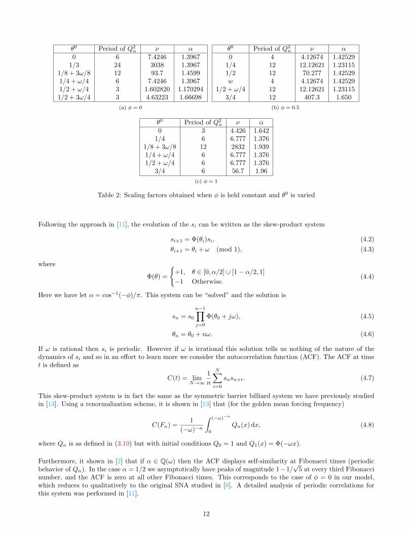
θ0 Period of Q2n ν α

0 6 7.4246 1.39671/3 24 3038 1.3967

1/8 + 3ω/8 12 93.7 1.45991/4 + ω/4 6 7.4246 1.39671/2 + ω/4 3 1.602820 1.1702941/2 + 3ω/4 3 4.63223 1.66698

(a) φ = 0

θ0 Period of Q2n ν α

0 4 4.12674 1.425291/4 12 12.12621 1.231151/2 12 70.277 1.42529w 4 4.12674 1.42529

1/2 + ω/4 12 12.12621 1.231153/4 12 407.3 1.650

(b) φ = 0.5

θ0 Period of Q2n ν α

0 3 4.426 1.6421/4 6 6.777 1.376

1/8 + 3ω/8 12 2832 1.9391/4 + ω/4 6 6.777 1.3761/2 + ω/4 6 6.777 1.376

3/4 6 56.7 1.96

(c) φ = 1

Table 2: Scaling factors obtained when φ is held constant and θ0 is varied

Following the approach in [11], the evolution of the si can be written as the skew-product system

si+1 = Φ(θi)si, (4.2)

θi+1 = θi + ω (mod 1), (4.3)

where

Φ(θ) =

{+1, θ ∈ [0, α/2] ∪ [1− α/2, 1]

−1 Otherwise.(4.4)

Here we have let α = cos−1(−φ)/π. This system can be “solved” and the solution is

sn = s0

n−1∏j=0

Φ(θ0 + jω), (4.5)

θn = θ0 + nω. (4.6)

If ω is rational then si is periodic. However if ω is irrational this solution tells us nothing of the nature of thedynamics of si and so in an effort to learn more we consider the autocorrelation function (ACF). The ACF at timet is defined as

C(t) = limN→∞

1

n

N∑i=0

snsn+t. (4.7)

This skew-product system is in fact the same as the symmetric barrier billiard system we have previously studiedin [13]. Using a renormalization scheme, it is shown in [13] that (for the golden mean forcing frequency)

C(Fn) =1

(−ω)−n

∫ (−ω)−n

0

Qn(x) dx, (4.8)

where Qn is as defined in (3.10) but with initial conditions Q0 = 1 and Q1(x) = Φ(−ωx).

Furthermore, it shown in [2] that if α ∈ Q(ω) then the ACF displays self-similarity at Fibonacci times (periodicbehavior of Qn). In the case α = 1/2 we asymptotically have peaks of magnitude 1−1/

√5 at every third Fibonacci

number, and the ACF is zero at all other Fibonacci times. This corresponds to the case of φ = 0 in our model,which reduces to qualitatively to the original SNA studied in [8]. A detailed analysis of periodic correlations forthis system was performed in [11].

12

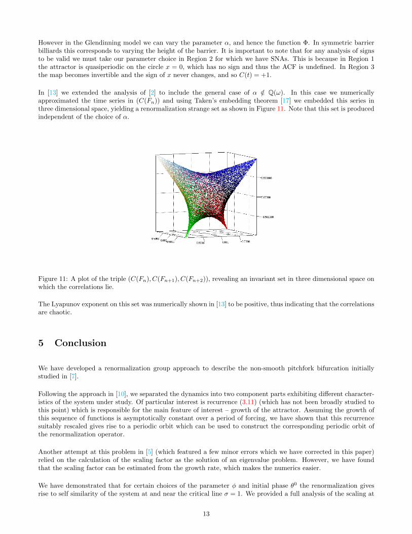
However in the Glendinning model we can vary the parameter α, and hence the function Φ. In symmetric barrierbilliards this corresponds to varying the height of the barrier. It is important to note that for any analysis of signsto be valid we must take our parameter choice in Region 2 for which we have SNAs. This is because in Region 1the attractor is quasiperiodic on the circle x = 0, which has no sign and thus the ACF is undefined. In Region 3the map becomes invertible and the sign of x never changes, and so C(t) = +1.

In [13] we extended the analysis of [2] to include the general case of α /∈ Q(ω). In this case we numericallyapproximated the time series in (C(Fn)) and using Taken’s embedding theorem [17] we embedded this series inthree dimensional space, yielding a renormalization strange set as shown in Figure 11. Note that this set is producedindependent of the choice of α.

Figure 11: A plot of the triple (C(Fn), C(Fn+1), C(Fn+2)), revealing an invariant set in three dimensional space onwhich the correlations lie.

The Lyapunov exponent on this set was numerically shown in [13] to be positive, thus indicating that the correlationsare chaotic.

5 Conclusion

We have developed a renormalization group approach to describe the non-smooth pitchfork bifurcation initiallystudied in [7].

Following the approach in [10], we separated the dynamics into two component parts exhibiting different character-istics of the system under study. Of particular interest is recurrence (3.11) (which has not been broadly studied tothis point) which is responsible for the main feature of interest – growth of the attractor. Assuming the growth ofthis sequence of functions is asymptotically constant over a period of forcing, we have shown that this recurrencesuitably rescaled gives rise to a periodic orbit which can be used to construct the corresponding periodic orbit ofthe renormalization operator.

Another attempt at this problem in [5] (which featured a few minor errors which we have corrected in this paper)relied on the calculation of the scaling factor as the solution of an eigenvalue problem. However, we have foundthat the scaling factor can be estimated from the growth rate, which makes the numerics easier.

We have demonstrated that for certain choices of the parameter φ and initial phase θ0 the renormalization givesrise to self similarity of the system at and near the critical line σ = 1. We provided a full analysis of the scaling at

13

the PCP, which is of interest as it separates three regimes of dynamical behaviour.

Finally, we provided a link between the autocorrelation function seen in the study of symmetric barrier billiards[13] and that seen for the study of signs in the Glendinning model. We show that the two systems in this contextare equivalent and that for a typical choice of parameter in Region 2 the correlations at Fibonacci times lie on arenormalization strange set which is the quasiperiodic equivalent to the so-called “orchid” set which occurs in thestudy of decaying eigenfunctions of the generalised Harper equation [12].

A generalization of this work to a class of quadratic irrational forcing frequencies should be straightforward. In [1]we extended our work on renormalization of the autocorrelation function in symmetric barrier billiards to such aclass of frequency, and the renormalization equations for Qn for the Glendinning model will be identical to thosein [1]. Indeed, the results from [1] can be directly ported over to the study of the autocorrelation function for theGlendinning model as shown in Section 4. Extending further to general irrational frequencies is more challenging asthe renormalization equations change at every step, depending on the continued fraction expansion of the frequency.

References

[1] L N C Adamson and A H Osbaldestin, Renormalisation of correlations in a barrier billiard: Quadratic irrationaltrajectories, Physica D: Nonlinear Phenomena 270 (2014), 30–45.

[2] J R Chapman and A H Osbaldestin, Self-similar correlations in a barrier billiard, Physica D 180 (2003), no. 1,71–91.

[3] M. Ding, C. Grebogi, and E Ott, Evolution of attractors in quasiperiodically forced systems: From quasiperiodicto strange nonchaotic to chaotic, Physical Review A 39 (1989), no. 5, 2593.

[4] T. A Driscoll, N. Hale, and L. N. Trefethen, Chebfun guide, Pafnuty Publications, 2014.

[5] U Feudel, S P Kuznetsov, and A Pikovsky, Strange nonchaotic attractors: Dynamics between order and chaosin quasiperiodically forced systems, World Scientific, Singapore, 2006.

[6] U Feudel, A Pikovsky, and A Politi, Renormalization of correlations and spectra of a strange non-chaoticattractor, Journal of Physics A: Mathematical and General 29 (1996), no. 17, 5297–5311.

[7] P Glendinning, The nonsmooth pitchfork bifurcation, Discrete & Continuous Dynamical Systems Series B 6(2004), no. 4, 457–464.

[8] C. Grebogi, E. Ott, S. Pelikan, and J. A Yorke, Strange attractors that are not chaotic, Physica D 13 (1984),no. 1, 261–268.

[9] G Keller, A note on strange nonchaotic attractors, Fundamenta Mathematicae 151 (1996), no. 2, 139–148.

[10] S P Kuznetsov, A S Pikovsky, and U Feudel, Birth of a strange nonchaotic attractor: A renormalization groupanalysis, Physical Review E 51 (1995), no. 3, R1629–R1632.

[11] B D Mestel and A H Osbaldestin, Periodic orbits of renormalisation for the correlations of strange nonchaoticattractors., Mathematical Physics Electronic Journal [electronic only] 6 (2000), no. 5, 27.

[12] , Golden mean renormalization for a generalized Harper equation: The Ketoja–Satija orchid, Journal ofMathematical Physics 45 (2004), 5042–5075.

[13] A H Osbaldestin and L N C Adamson, Chaotic correlations in barrier billiards with arbitrary barriers, Journalof Physics A: Mathematical and Theoretical 46 (2013), no. 24, 245101.

[14] A S Pikovsky and U Feudel, Correlations and spectra of strange nonchaotic attractors, Journal of Physics A:Mathematical and General 27 (1994), no. 15, 5209–5219.

[15] , Characterizing strange nonchaotic attractors, Chaos: An Interdisciplinary Journal of Nonlinear Science5 (1995), no. 1, 253–260.

14

[16] F J Romeiras, A Bondeson, E Ott, T M Antonsen Jr, and C Grebogi, Quasiperiodic forcing and the observabilityof strange nonchaotic attractors, Physica Scripta 40 (1989), no. 3, 442.

[17] F Takens, Detecting strange attractors in turbulence (Lecture Notes Mathematics vol 898), Berlin: Springer(1981), 366–381.

15