Hopf Bifurcation and Chaotic Response in Nonlinear ...Hopf Bifurcation and Chaotic Response in Nonlinear ... rate recurrent neural networks are used to study the neuronal behaviour

Volume III, Issue V, May 2016 IJRSI ISSN 2321 – 2705

www.rsisinternational.org Page 67

Hopf Bifurcation and Chaotic Response in Nonlinear

Dynamics of Firing-Rate Recurrent Networks of Neurons

Abhishek Yadav*1

, Anurag Kumar Swami*, Ajay Srivastava

* *Department of Electrical Engineering,

College of Technology, G.B. Pant University of Agriculture & Technology, Pantnagar-263145, INDIA

Abstract— In-depth analysis of the nonlinear dynamics and chaotic

behaviour of interconnection of neurons has been made in order to

investigate the learning capabilities of this interconnection. Firing-

rate recurrent neural networks are used to study the neuronal

behaviour in a population of neurons. Dynamical behaviour of

these network models is investigated in order to seek their

capability to represent the presence of chaos in nervous system.

Study of chaos and other phenomena of nonlinear dynamics in

these network models can provide a significant help in

investigating the learning mechanism. It is found that the response

of the network highly depends on its parameters. Such type of model

exhibits all types of dynamics namely converging, oscillatory, and

chaotic with the variation in the synaptic weights.

Keywords— Recurrent Neural Networks, Firing Rate,

Nonlinear Dynamics, Hopf Bifurcation, Chaos.

I. INTRODUCTION

he brain is one of the most complex objects in the

universe. Although many attempts have been made to

investigate and model the functionalities of the brain, the

exact working of it is still unknown. The research in the field

of computational neuroscience is aimed to know about the

brain with more intricacy and to develop more realistic

models of its constituents. These models are important tools

for characterizing what nervous systems do, determining how

they function, and understanding why they operate in

particular ways. As most of these models are dynamical in

nature, theory of dynamical systems is useful in gaining new

insights into the operation of nervous system. The primary

step for understanding the brain dynamics is to understand

the dynamical behaviour of mathematical models of

individual neurons. The most important part of this study is

the bifurcation analysis of the neurons and their networks.

Certain bifurcations in the membrane potential result in

neural excitability, spiking, and bursting. Revealing these

bifurcations in neuron models helps in knowing various

functions of the brain. Such types of studies include the

analysis of chaotic behaviour of neural systems. These

neural systems can be individual neurons or their

interconnections. The ongoing research in this regard is to

examine the role of chaos in learning. Exploring dynamics

of biological neuron models is helpful not only in

neuroscience studies but also in neural network applications.

Capabilities of existing artificial neural networks are

extremely less as compared to that of a human brain.

Artificial neural networks mimic only a negligibly small part

of the actual activities in brain. It is logical to seek the

possibilities of improvements in artificial neural networks by

incorporating more of biological facts.

In literature, different dynamical models are proposed to

represent biophysical activities of neurons. Commonly used

models for the study of spiking and bursting behaviours of

neurons include integrate-and-fire model and its variants [5],

[25], FitzHugh-Nagumo model [6], Hindmarsh-Rose model

[14], [10], Hodgkin-Huxley model [10], [11], and Morris-Lecar

model [20]. A short review of these models is provided by

Rinzel in [21] - [23]. An excellent comparison of more than

twenty neurocomputational properties of the most popular

spiking and bursting models have been made in [14].

Bifurcation phenomena in individual neuron models including

the Hodgkin-Huxley, Morris-Lecar and FitzHugh-Nagumo

models have been investigated in the literature [14], [22], [4].

Rinzel and Ermentrout [22] studied bifurcations in the Morris-

Lecar model by treating the externally applied direct current as

a bifurcation parameter. Effect of noise on the dynamics of

biological neuron models has been investigated in [19].

After studying the dynamics of individual neurons, the next

step to study brain dynamics is to analyse the neuronal

behaviour in a network of neurons. A neuron communicates

with other neurons via electrical impulses called spikes. From

various experiments, it has been well established that neuronal

activities show many characteristics of chaotic behaviour.

Some researchers believe that this sort of behaviour is

necessary for the brain to engage in continual learning –

categorizing a novel input into a novel category rather than

trying to fit it into an existing category [24], [8], [1].

Freeman developed a mathematical model for EEG signals

generated by the olfactory system in rabbits [8]. He suggested

that the learning and recognition of novel odours, as well as

the recall of familiar odours can be explained through

chaotic dynamics of the olfactory cortex. Chaotic response in

the models of single neurons has been observed in [17] and a

similar analysis on coupled neurons has been performed in

[18]. Attempts have been made to represent the neuronal

dynamics of biological neural networks in terms of artificial

neural network type of structures with some extent to their

intricacies. Chaotic dynamics based neural networks have also

been proposed to capture some of the characteristics of learning

in the brain [2].

In this paper work, nonlinear dynamical analysis of a

T



firing-rate recurrent neural network of three neurons has

been carried out and it is observed that its dynamical

behaviour exhibits Hopf bifurcation and becomes chaotic at

some set of parametric values. This study supports the role

of chaos in continual learning– categorizing a novel input

into a novel category rather than trying to fit it into an

existent category.

II. INTRODUCTION TO NONLINEAR DYNAMICS

AND CHAOS

A dynamical system consists of a rule which specifies

how a system evolves and an initial condition at which the

system starts. The most common form of rules is a set of

differential equations [21]. A dynamical system is said to be

nonlinear if it is described by nonlinear differential

equations. A nonlinear system exhibits various types of

dynamics including converging, oscillatory and chaotic. For

dynamical analysis of nonlinear systems, eigenvalue

analysis, Lyapunov exponents, and bifurcation diagrams are

three major tools. These tools are used to detect the

qualitative change in the dynamical behaviour of the system

when a parameter is changed. This phenomenon is called

bifurcation.

A. Eigenvalue Analysis

Consider the following nonlinear dynamical system

dx(t)/dt = F(x(t); µ) (1)

where x(t) = x1(t), x2(t), ....., xn(t) is the state vector

and µ is a parameter. Equilibrium points are obtained

from the condition dx/dt = 0. Therefore, for any µ, the equilibrium point xe(µ) satisfy the following algebraic

equation

F (xe(µ); µ) = 0 (2)

Jacobian matrix evaluated at the equivalent point is

J(µ). Eigenvalues λ1, λ2, ..., λn are the roots of the

characteristic equation

det (λI − J(µ)) = 0 (3)

where I is the n × n identity matrix. Suppose in a neighbourhood of a particular value µ0 of the parameter

µ there is a pair of eigenvalues of J(µ) of the form λreal

(µ) ± iλimag(µ) such that λreal (µ0) = 0, λimag (µ0)

= 0, no other eigenvalue of J(µ0) has a pair of pure

imaginary eigenvalues. Suppose further that the rate of change of the real part of eigenvalues is nonzero at µ0,

i.e.,

dλreal / dµ (at µ = µ0) = 0 (4)

then a limit cycle bifurcates from the origin with an

amplitude that grows proportional to |µ|½

while its period tends to 2π/λimag as µ → µ0. This bifurcation is

called Hopf bifurcation.

B. Lyapunov Exponents

Trajectories of chaotic systems are very sensitive to the

initial conditions. Starting from slightly different initial

conditions the trajectories diverge exponentially. Let d0

denote the distance between the two initial states of a

continuous dynamical system. Then, for a chaotic motion, at

a later time,

d(t) = eµt

d0 (5)

The measure of the divergence of trajectories is

obtained by averaging the exponential growth at many

points along a trajectory [27]. To define this, first a

reference trajectory is obtained. Then, a point on an

adjacent trajectory is selected and d(t)/d0 is measured.

After this, a new d0(t) is selected on new adjacent

trajectory. Lyapunov exponent is computed as

𝜇 𝑥 0 = lim𝑁→∞1

𝑡𝑁−𝑡0 𝑙𝑛

𝑑 𝑡𝑘

𝑑0 𝑡𝑘−1 𝑁𝑘=1 (6)

There are n Lyapunov exponents for an n-dimensional

nonlinear dynamical system. To define these Lyapunov

exponents, an n dimensional sphere cantered at a point on a

reference trajectory is chosen. Let the radius of this trajectory be δ0. At a later time, an n-dimensional ellipsoid

is constructed with the property that all the trajectories

emanating from the previously chosen sphere pass through

this ellipsoid. Let the n semiaxes of the ellipsoid be denoted by δi(t), Lyapunov exponent is computed as

𝜇 𝑥 0 = lim𝑡→∞

lim𝛿𝑖 0 →0

1

𝑡𝑙𝑛

𝛿𝑖 𝑡

𝛿𝑖 0 ; 𝑖 = 1,2, …… , 𝑛

(7)

A system is chaotic if there exists at least one positive

Lyapunov exponent. Plot of the largest Lyapunov exponent

with respect to the bifurcation parameter gives the range

of the parameter for which there exists at least one positive

Lyapunov exponent. Thus, system exhibits chaotic behaviour

for this range of the parameter.

C. Bifurcation Diagram

Bifurcation diagrams are pictorial representation of

qualitative change in the dynamical behaviour of a system

when a parameter is varied. This parameter is called

bifurcation parameter and its values at which bifurcation

takes place are called bifurcation points. The horizontal

axis of a bifurcation diagram has the parameter and the



vertical axis has some aspect of the solution, such as,

the norm of the solution, the maximum and/or

minimum values of one of the state variables, the

frequency of a solution, or the average of one of the state

variables.

III. DYNAMICAL ANALYSIS OF FIRING-RATE

RECURRENT NEURAL NETWORK

Firing-rate recurrent neural networks are used to study

the neuronal behaviour in a population of neurons.

Dynamical behaviour of these network models is

investigated in order to seek their capability to represent

the presence of chaos in nervous system. Study of chaos

and other phenomena of nonlinear dynamics in these

network models can provide a significant help in

investigating the learning mechanism. It is found that

the response of the network highly depends on its

parameters. Such type of model exhibits all types of

dynamics namely converging, oscillatory and chaotic with

the variation in the synaptic weights.

A. Models of Biological Neural Networks

Widespread synaptic connectivity is a characteristic

of neural circuitry. Network models permit us to

discover the computational potential of such

connectivity, using both analysis and simulations.

These networks have been considered to investigate the

various tasks performed by them. These tasks include

coordinate transformations needed in visually guided

reaching, discriminatory amplification leading to models

of simple and complex cells in primary visual cortex,

amalgamation as a model of short-term memory, noise

reduction, input selection, gain modulation, and

associative memory [3]. There are two ways to simulate

neural networks: one is based on the action potential and

another one is based upon the firing rate. The first one

presents noteworthy computational and interpretational

challenges. Firing-rate models avoid the short time scale

dynamics required to simulate action potentials and

thus are much easier to simulate on computers [2].

B. Firing Rate Models

The construction of a firing-rate model proceeds in two

steps. First, it is determine how the total synaptic input to

a neuron depends on the firing rates of its presynaptic

afferents. This is where the firing rates are used to

approximate neural network functions. Second, the

dependency of firing rate of the postsynaptic neuron on its

total synaptic input is formed. Firing rate response curves

are usually measured by injecting current (Is) into the

soma of a neuron. Letter u is used to symbolize a

presynaptic firing rate and v to symbolize a postsynaptic

rate [3].

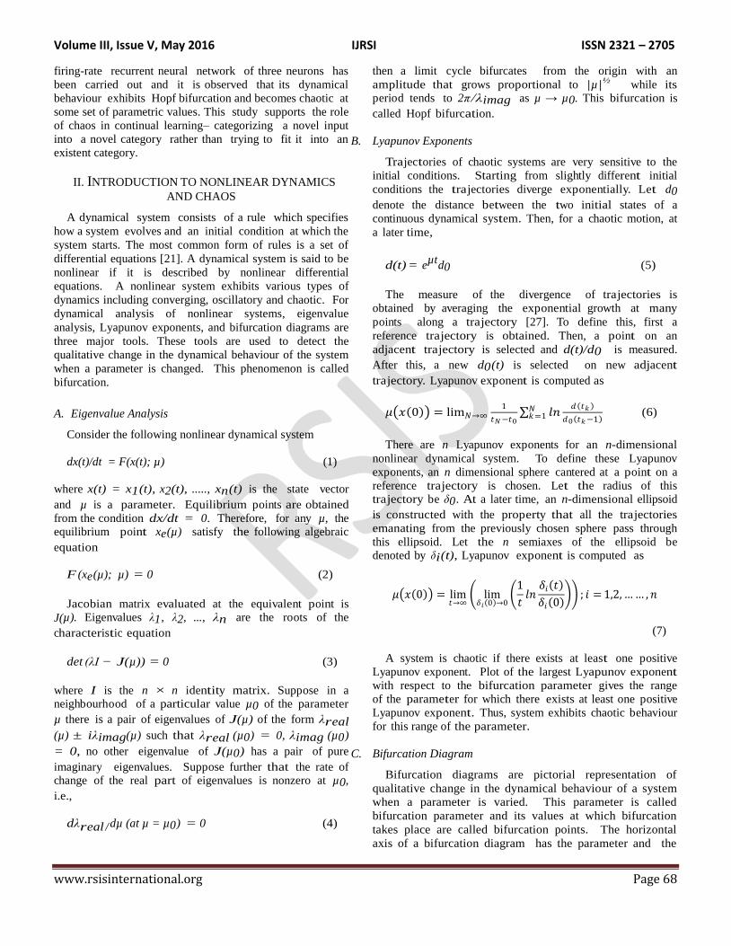
C. Feedforward and Recurrent Networks

Examples of network models with feedforward and

recurrent connectivity are shown in Figure 1. The

feedforward network of Figure 1(a) has Nv output units

with rates vi (i = 1, 2, 3, ....., Nv), denoted jointly by v

determined by Nu input units with rates ui (i = 1, 2, 3,

......, Nu), denoted jointly by u. The output firing rates are

then determined by Equations 8 and 9.

𝜏𝑟𝜕𝑣𝑖

𝜕𝑡= −𝑣𝑖 + 𝐹 𝑊𝑖𝑗𝑢𝑗

𝑁𝑢𝑗=1 (8)

𝜏𝑟𝜕𝒗

𝜕𝑡= −𝒗 + 𝐹 𝑾. 𝒖 (9)

where F is any activation function. It is commonly taken

to be a saturating function such as a sigmoid function.

The recurrent network of Figure 1(b) also has two layers of

neurons with rates u and v, but in this case the neurons of

the output layer are interconnected with synaptic weights

described by a matrix w. Matrix element wij0 describes

the strength of the synapse from the output unit j0 to

output unit i. The output rates in this case are determined

by Equations 10 and 11.

𝜏𝑟𝜕𝑣𝑖

𝜕𝑡= −𝑣𝑖 + 𝐹 𝑊𝑖𝑗𝑢𝑗

𝑁𝑢𝑗=1 + 𝑤𝑖𝑗 ′𝑣𝑗 ′

𝑁𝑣𝑗 ′=1 (10)

𝜏𝑟𝜕𝒗

𝜕𝑡= −𝒗 + 𝐹 𝑾. 𝒖 + 𝒘. 𝒗 (11)

A firing-rate recurrent neural network with Nv = 3 and

W = 0 is considered for this study. Dynamics of this model

is studied at different values of synaptic strength w.

Condition for Hopf bifurcation is determined with the help

of eigenvalue analysis of the linearized system around its

equilibrium points. The presence of chaos is investigated by

calculating the largest Lyapunov exponent and plotting

bifurcation diagram, time responses and phase portraits at

some relevant values of parameters. The nonlinear

differential equations for the above model are given in

Equations 12-14.

(a) Feedforward network



(b) Recurrent network

Fig. 1. Feedforward and Recurrent networks. In the case of feedforward networks, the neurons of the output layer are not

interconnected while they are interconnected with synaptic weights

in case of the recurrent network.

𝜕𝑥 (𝑡)

𝜕𝑡= 𝑓1(𝑤12𝑦 𝑡 + 𝑤13𝑧 𝑡 ) − 𝛼1𝑥 𝑡 (12)

𝜕𝑥 (𝑡)

𝜕𝑡= 𝑓2(𝑤21𝑥 𝑡 + 𝑤23𝑧 𝑡 ) − 𝛼2𝑦 𝑡 (13)

𝜕𝑧 (𝑡)

𝜕𝑡= 𝑓3(𝑤31𝑥 𝑡 + 𝑤32𝑦 𝑡 ) − 𝛼3𝑧 𝑡 (14)

The response function fi is given in Equation 15.

𝑓𝑖 𝑠 =1

1+𝑒−𝛽𝑖(𝑠−𝜃𝑖) (15)

x(t), y(t), and z(t) are the output spike-rates (i.e.,

elements of v) of neurons represented by subscripts 1,

2, and 3 respectively. These quantities are

interpretable as short-term average of firing-rates of

respective neurons. θi is the threshold and βi is the

slope of transfer function of neuron i. αi is the decay

rate of the neuron i. wij is the synaptic strength of

the connection from neuron j to neuron i.

D. Eigenvalue Analysis of the Model

The equilibrium state (xe, ye, ze) of the system is

given by the solution of the following set of equations

𝑓1(𝑤12𝑦𝑒 𝑡 + 𝑤13𝑧𝑒 𝑡 ) − 𝛼1𝑥𝑒 𝑡 = 0 (16)

𝑓2(𝑤21𝑥𝑒 𝑡 + 𝑤23𝑧𝑒 𝑡 ) − 𝛼2𝑦𝑒 𝑡 = 0 (17)

𝑓3(𝑤31𝑥𝑒 𝑡 + 𝑤32𝑦𝑒 𝑡 ) − 𝛼3𝑧𝑒 𝑡 = 0 (18)

Linearizing the system around the equilibrium

points (xe, ye, ze), we get the following system matrix:

𝐽 =

−α1 − u β1w12 a β1w13

aβ2w21 b −α2 −u β2w23 bβ3 w31 c β3w32 c −α3 − u

where

𝑎 = 𝐹 𝛽1 𝑤12 𝑦𝑒 + 𝑤13 𝑧𝑒 − 𝜃1

𝑏 = 𝐹 𝛽1 𝑤21 𝑥𝑒 + 𝑤23 𝑧𝑒 − 𝜃2

𝑐 = 𝐹 (𝛽1(𝑤31 𝑥𝑒 + 𝑤32 𝑦𝑒) − 𝜃3 )

Here, F(a) is given by

𝐹 𝑎 =𝑒−𝑎

(1+𝑒−𝑎 )2 (19)

We can form the characteristic equation by

substituting the above matrix J in |λI − J | = 0. Thus,

we get the following characteristic equation

λ3

+ Aλ2

+ Bλ + C = 0……..(20)

where A = α1 + α2 + α3

B = α1α2 + α2α3 + α1α3 − (β1 β2 w12 w21 ab + β2β3 w23 w32 bc + β1β3w31 w13 ca)

C = α1 α2 α3 − (α3β1 β2 w12 w21 ab + α2β3 β1w31 w13 bc + α1β3β2w23 w32 ac)

− β1β2 β3 abc (w23 w31 w13 + w21 w32 w13)

By applying Routh-Hurwitz criterion to

investigate the values of A, B and C , for Hopf

bifurcation, it is found that the system exhibits Hopf

bifurcation if A = 0, AB − C = 0 or C = 0. w13 is

considered as bifurcation parameter. Following values

of other parameters are used: β1 = 7, β2 = 7, β3 =

15, θ1 = 0.5, θ2 = 0.3, θ3 = 0.7, α1 = 0.65, α2 = 0.42, α3

= 0.1, w12 = 1, w21 = 1, w23 = 0.1, w31 = 1 and w32 =

0.02. Therefore, at these values of parameters, A, AB –

C and C are plotted against the bifurcation parameter

w13 as shown in Figure 2. It is observed that at w13 =

−5.2, AB − C becomes zero. This indicates the

possibility of Hopf bifurcation which is confirmed from

time responses and phase portraits.

Fig. 2. Plots of A, AB – C, and C of the Routh array with respect

to w13 . A, B, and C are the coefficients of the characteristic equation

of the firing-rate recurrent neural network. It is observed that at



w13 = −5.2, AB − C becomes zero and therefore Hopf

bifurcation takes place at this value of w13 .

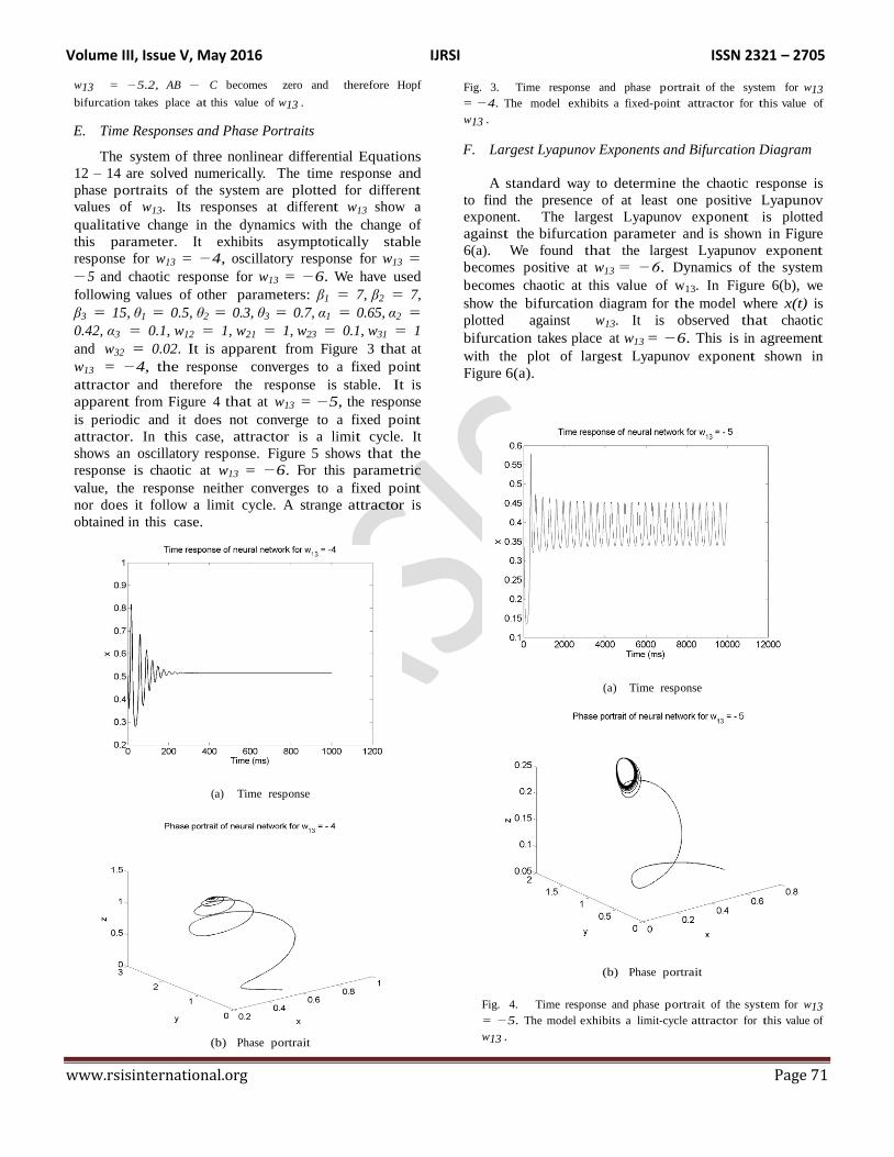
E. Time Responses and Phase Portraits

The system of three nonlinear differential Equations

12 – 14 are solved numerically. The time response and

phase portraits of the system are plotted for different

values of w13. Its responses at different w13 show a

qualitative change in the dynamics with the change of

this parameter. It exhibits asymptotically stable

response for w13 = −4, oscillatory response for w13 =

−5 and chaotic response for w13 = −6. We have used

following values of other parameters: β1 = 7, β2 = 7,

β3 = 15, θ1 = 0.5, θ2 = 0.3, θ3 = 0.7, α1 = 0.65, α2 =

0.42, α3 = 0.1, w12 = 1, w21 = 1, w23 = 0.1, w31 = 1

and w32 = 0.02. It is apparent from Figure 3 that at

w13 = −4, the response converges to a fixed point

attractor and therefore the response is stable. It is

apparent from Figure 4 that at w13 = −5, the response

is periodic and it does not converge to a fixed point

attractor. In this case, attractor is a limit cycle. It

shows an oscillatory response. Figure 5 shows that the

response is chaotic at w13 = −6. For this parametric

value, the response neither converges to a fixed point

nor does it follow a limit cycle. A strange attractor is

obtained in this case.

(a) Time response

(b) Phase portrait

Fig. 3. Time response and phase portrait of the system for w13

= −4. The model exhibits a fixed-point attractor for this value of

w13 .

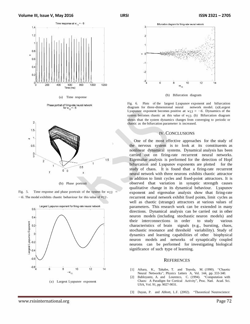
F. Largest Lyapunov Exponents and Bifurcation Diagram

A standard way to determine the chaotic response is

to find the presence of at least one positive Lyapunov

exponent. The largest Lyapunov exponent is plotted

against the bifurcation parameter and is shown in Figure

6(a). We found that the largest Lyapunov exponent

becomes positive at w13 = −6. Dynamics of the system

becomes chaotic at this value of w13. In Figure 6(b), we

show the bifurcation diagram for the model where x(t) is

plotted against w13. It is observed that chaotic

bifurcation takes place at w13 = −6. This is in agreement

with the plot of largest Lyapunov exponent shown in

Figure 6(a).

(a) Time response

(b) Phase portrait

Fig. 4. Time response and phase portrait of the system for w13

= −5. The model exhibits a limit-cycle attractor for this value of

w13 .



(a) Time response

(b) Phase portrait

Fig. 5. Time response and phase portrait of the system for w13 =

−6. The model exhibits chaotic behaviour for this value of w13 .

(a) Largest Lyapunov exponent

(b) Bifurcation diagram

Fig. 6. Plots of the largest Lyapunov exponent and bifurcation

diagram for three-dimensional neural network model. (a)Largest

Lyapunov exponent becomes positive at w13 = −6. Dynamics of the

system becomes chaotic at this value of w13. (b) Bifurcation diagram

shows that the system dynamics changes from converging to periodic or chaotic as the bifurcation parameter is increased.

IV. CONCLUSIONS

One of the most effective approaches for the study of

the nervous system is to look at its constituents as

nonlinear dynamical systems. Dynamical analysis has been

carried out on firing-rate recurrent neural networks.

Eigenvalue analysis is performed for the detection of Hopf

bifurcation and Lyapunov exponents are plotted for the

study of chaos. It is found that a firing-rate recurrent

neural network with three neurons exhibits chaotic attractor

in addition to limit cycles and fixed-point attractors. It is

observed that variation in synaptic strength causes

qualitative change in its dynamical behaviour. Lyapunov

exponent and eigenvalue analysis show that firing-rate

recurrent neural network exhibit fixed points, limit cycles as

well as chaotic (strange) attractors at various values of

parameters. This research work can be extended in many

directions. Dynamical analysis can be carried out in other

neuron models (including stochastic neuron models) and

their interconnections in order to study various

characteristics of brain signals (e.g., bursting, chaos,

stochastic resonance and threshold variability). Study of

dynamics and learning capabilities of other biophysical

neuron models and networks of synaptically coupled

neurons can be performed for investigating biological

significance of such type of learning.

REFERENCES

[1] Aihara, K., Takabe, T. and Toyoda, M. (1990). ―Chaotic

Neural Networks‖, Physics Letters A, Vol. 144, pp. 333-340.

[2] Babloyantz, A. and Lourenco, C. (1994). ―Computation with

Chaos: A Paradigm for Cortical Activity‖, Proc. Natl. Acad. Sci. USA, Vol. 91, pp. 9027-9031.

[3] Dayan, P. and Abbott, L.F. (2002). ―Theoretical Neuroscience:



Computational and Mathematical Modelling of Neural Systems‖, The MIT Press, Cambridge, Massachusetts, London, England.

[4] Ehibilik, A.I., Borisyuk, R.M. and Roose, D. (1986). ―Numerical

Bifurcation Analysis of a Model of Coupled Neural Oscillators‖,

International Series of Numerical Mathematics, Vol. 104, pp. 215–

228, 1992. Ermentrout, G.B. and Kopell, N. ―Parabolic Bursting in

an Excitable System Coupled with a Slow Oscillation‖, SIAM Journal on Applied Mathematics, Vol. 46, pp. 233–253.

[5] Ermentrout, G.B. (1996). ―Type I Membranes, Phase Resetting

Curves and Synchrony‖, Neural Computing, Vol. 8, pp. 979–1001. [6] FitzHugh, R. (1961). ―Impulses and Physiological States in Models

of Nerve Membrane‖, Biophysical Journal, Vol. 1, pp.445–466.

[7] FitzHugh, R. (1969). ―Mathematical Models for Excitation and Propagation in Nerve‖, Biological Engineering H.P. Schawn (Ed.),

New York: McGraw-Hill.

[8] Freeman W.J. (1987). ―Simulation of Chaotic EEG Patterns with a Dynamic Model of the Olfactory System‖, Biological Cybernetics,

pp. 139–150.

[9] Hindmarsh, J.L. and Rose, R.M. (1984). ―A Model of Neuronal Bursting Using Three Coupled First Order Differential

Equations‖, Proc. R. Soc. Lond. Biol., Vol. 221, pp. 87-102.

[10] Hodgkin, A. and Huxley, A. (1952). ―A Quantitative Description of Membrane Current and Its Application to Conduction and

Excitation in Nerve‖, J.Phisiol., (Lond.), Vol. 117, pp. 500–544.

[11] Hodgkin, A.L. and Huxley, A.F. (1954). ―A Quantitative Description of Membrane Current and Application to

Conduction and Excitation in Nerve‖, Journal of Physiology, Vol.

117, pp. 500–544. [12] Hodgkin, A.L. (1948). ―The Local Changes Associated with

Repetitive Action in a Non-Modulated Axon‖ Journal of

Physiology, Vol. 107, pp. 165–181. [13] Hoppensteadt, F.C. and Izhikevich, E.M. (2000). ―Weakly

Connected Neural Networks‖, Springer-Verlag, 1997. Izhikevich,

E.M. ―Neural Excitability, Spiking and Bursting‖, International Journal of Bifurcation and Chaos, Vol. 10, pp. 1171–1266.

[14] Izhikevich, E.M. (2004). ―Which Model to Use for Cortical

Spiking Neurons?‖, IEEE Transaction on Neural Networks, Vol. 15, pp. 1063-1070.

[15] Koch, C. and Poggio, T. (1992). ―Multiplying with Synapses and

Neurons‖, Single Neuron Computation, Academic Press: Boston, Massachusetts, pp. 315-315.

[16] Koch C. (1999). ―Biophysics of Computation: Information Processing

in Single Neurons‖, Oxford University Press.

[17] Mishra, D, Yadav, A, Ray, S. and Kalra, P.K. (2004). ―Nonlinear

Dynamical Analysis of Single Neuron Models and Study of Chaos in

Brain‖, Proceedings of International Conference on Cognitive Science, Allahabad, pp 188 - 193.

[18] Mishra, D, Yadav, A, Ray, S. and Kalra, P.K. (2005). ―Effects of

Noise on the Dynamics of Biological Neuron Models‖, Proceedings of the Fourth IEEE International Workshop WSTST05, Muroran

(Japan), pp 61 - 69.

[19] Mishra, D, Yadav, A, Ray, S. and Kalra, P.K. (2005). ―Nonlinear Dynamical Analysis on Coupled Modified FitzHugh-

Nagumo Neuron Model‖, Proceedings of International Symposium of

Neural Network 2005, Chongqing (China). [20] Morris, C. and Lecar, H. (1981). ―Voltage Oscillations in the

Barnacle Giant Muscle Fiber‖, Journal of Biophysics, Vol. 35, pp.

193–213. [21] Rinzel, J. (1981). ―Models in Neurobiology‖, Nonlinear Phenomena

in Physics and Biology, Plenum Press, New York, 345–367.

[22] Rinzel, J. and Ermentrout, G.B. (1989). ―Analysis of Neural Excitability and Oscillations‖, Methods in Neuronal Modeling, MIT

press, Cambridge MA.

[23] Rinzel, J. (1987). ―A Formal Classification of Bursting Mechanisms in Excitable Systems, in Mathematical Topics in Population Biology,

Morphogenesis and Neurosciences‖, Lecture Notes in

Biomathematics, Springer- Verlag, New York, Vol. 71, pp. 267–281. [24] Skarda, C.A. and Freeman, W.J. (1987). ―How brains make chaos in

order to make sense of the world‖, Behavioral Brain Science Vol. 10,

pp. 161–195. [25] Tuckwell, H. C. (1988). ―Introduction to Theoretical Neurobiology‖,

Cambridge University Press.

[26] Wilson, H. (1999). ―Simplified Dynamics of Human and Mammalian Neocortical Neurons‖, Journal of Theoretical Biology, Vol. 200, pp.

375-388.

[27] Zak, S. H. (2002). ―Systems and Control‖, Oxford University Press, ISBN:0195150112.

Documents

Hopf Bifurcation and Chaotic Response in Nonlinear ...Hopf Bifurcation and Chaotic Response in Nonlinear ... rate recurrent neural networks are used to study the neuronal behaviour