ON THE HAUSDORFF DIMENSION OF CAT SURFACES

ON THE HAUSDORFF DIMENSION OF CAT(κ) SURFACES

DAVID CONSTANTINE AND JEAN-FRANCOIS LAFONT

Abstract. We prove that a closed surface with a CAT(κ) metric has Haus-dorff dimension = 2, and that there are uniform upper and lower bounds on

the two-dimensional Hausdorff measure of small metric balls. We also discuss

a connection between this uniformity condition and some results on the dy-namics of the geodesic flow for such surfaces. Finally, we give a short proof of

topological entropy rigidity for geodesic flow on certain CAT(−1) manifolds.

1. Introduction

Let Σ be a closed surface, κ any real number, and let d be a locally CAT(κ) metricon Σ. One quantity of natural interest is the Hausdorff dimension of (Σ, d), denoteddimH(Σ, d). This dimension is bounded below by 2, the topological (covering)dimension of Σ. However, for an arbitrary metric on Σ there is no upper bound; thiscan be seen by “snowflaking” the metric – replacing d(x, y) with d′(x, y) = d(x, y)αfor 0 < α < 1, which raises the Hausdorff dimension by a factor of 1/α (see, e.g.[TW05]). In this paper we examine the restriction placed on dimH(Σ, d) by theCAT(κ) condition, and prove the following theorem:

Theorem 1. Let (Σ, d) be a CAT(κ) closed surface. Then dimH(Σ, d) = 2. More-over, there exists some δ0 > 0 such that for all 0 < δ ≤ δ0,

infp∈Σ

H2(B(p, δ)) > 0 and supp∈Σ

H2(B(p, δ)) <∞

where H2 denotes the 2-dimensional Hausdorff measure and B(p, δ) is the ball ofradius δ around p.

We note that the second statement of the theorem implies the first, but notvice versa. Indeed there are metric spaces with Hausdorff dimension d whose d-dimensional Hausdorff measures are zero or infinite. We became interested in thisquestion for Hausdorff measures, in particular the uniform bounds on the measuresof balls, while thinking about some results on entropy for geodesic flows on locallyCAT(−1) manifolds. As an immediate application of Theorem 1, we have

Corollary 2. Let (Σ, d) be a closed surface with a CAT(0) metric. Let φt be thegeodesic flow on the space of geodesics for (Σ, d). Then the topological entropy forthe flow equals the volume growth entropy for the Hausdorff 2-measure.

Corollary 2 is a version of Manning’s [Man79] analogous result for Riemannianmanifolds of non-positive curvature, and relies on some work of Leuzinger [Leu06].This is discussed in the final section of the paper, where we also establish thefollowing entropy rigidity result for the geodesic flow.

Date: June 24, 2016.

1

2 DAVID CONSTANTINE AND JEAN-FRANCOIS LAFONT

Theorem 3. Let (X,d) be a closed CAT(−1) manifold (not necessarily Riemann-ian), and suppose that X admits a Riemannian metric g so that (X,g) is a locallysymmetric space. Let htop(φdt ) and htop(φgt ) be the topological entropies for thegeodesic flows under the two metrics. Then

htop(φdt ) ≥ htop(φgt )

and if equality holds, (X,d) is also locally symmetric. If dimX > 2, (X,d) and(X,g) are isometric.

Theorem 3 is a reformulation of a rigidity result of Bourdon ([Bou96]). Our mainobservation is to note how, using Leuzinger’s work [Leu06], Bourdon’s theorem canbe recast as a topological entropy rigidity theorem. This fact may well be knownto experts, but we have not found it addressed in the literature.

The paper is organized as follows. In Sections 2 and 3 we show that smalldistance spheres around each point in Σ are topological circles, and that they arerectifiable with bounded length. In Section 4 we prove Theorem 1, and in Section5 we discuss the extension of Theorem 1 to higher dimensions, and give an examplewhich indicates some of the complications in doing so. In Section 6 we give the proofof topological entropy rigidity (Theorem 3) for certain locally CAT(−1) manifolds.

Acknowledgements. We would like to thank Enrico Leuzinger and Mike Davis forhelpful conversations, as well as the anonymous referee for their careful reading. Thefirst author would like to thank Ohio State University for hosting him during thetime that most of this work was done. The second author was partially supportedby the NSF, under grant DMS-1510640.

2. The topology of small distance spheres

Let S(p, ε) = {z ∈ Σ ∶ d(p, z) = ε} and B(p, ε) = {z ∈ Σ ∶ d(p, z) ≤ ε} respectivelydenote the metric ε-sphere and ε-ball centered at p. In this section we prove forsmall ε, all S(p, ε) are topological circles. We note that the argument only works forsurfaces. In Section 5 we give examples of higher-dimensional CAT(−1) manifoldswhere the analogous statement is not true – small metric spheres need not betopological spheres.

Throughout this section, we work at small scale. We fix ε0 > 0 small enough sothat the following two conditions are satisfied:

● ε0 ≤Dκ/2 whereDκ is the diameter of the model space of constant curvatureκ, and

● For all p ∈ Σ, B(p, ε0) is (globally) CAT(κ).At these scales, B(p, ε0) is locally uniquely geodesic – in particular there is a uniquegeodesic from p to any point in B(p, ε0), which varies continuously with respect tothe endpoints. This will be a key fact in the work below. As a consequence, eachsuch ball B(p, ε0) is contractible, hence lifts isometrically to the universal cover

(Σ, d).The following Lemma will be useful. Its proof, which is straightforward and can

be adapted to any dimension, can be found in [BH99, Proposition II.5.12].

ON THE HAUSDORFF DIMENSION OF CAT(κ) SURFACES 3

Lemma 4. Let [xy] be a geodesic segment in Σ connecting an arbitrary pair ofpoints x and y. Then [xy] can be extended beyond y. That is, there is a geo-desic segment (not necessarily unique) [xy′] properly containing [xy] as its initialsegment.

Remark. Using the compactness of X, and a connectedness argument on R, thislemma implies that each geodesic segment [xy] can be infinitely extended.

The main result of this section is the following:

Proposition 5. Let Σ be a complete CAT(κ) surface. Then for all ε < ε0, S(p, ε)is homeomorphic to the circle S1.

In order to establish this result, we use a well-known characterization of thecircle S1. The circle is the only compact, connected, metric space (X,d) with theproperty that for any pair of distinct points a, b ∈ X, the complement X ∖ {a, b} isdisconnected (see, e.g [HY88, Theorem 2-28]). Let p ∈ Σ be an arbitrary point inΣ, and to simplify notation, we set Sε ∶= S(p, ε). We now claim that for ε < ε0, Sεis homeomorphic to a circle.

Lemma 6. For all ε < ε0, Sε is a compact, path-connected, metric space.

Proof. Sε is a closed subset of the compact metric space Σ, so it is compact andmetric. Since ε < ε0, Sε lifts homeomorphically to a subset of Σ. Since Σ is asurface, Σ is homeomorphic to R2 or S2, so we may take Sε to a be a compactsubset of R2 or S2.Sε has diameter <Dκ, so we may find a path S in R2 or S2 homeomorphic to S1

bounding a disk containing Sε and remaining in B(p, ε0). Let proj ∶ S → Sε be thenearest point projection (for the CAT(κ) metric lifted from Σ). This is well-defined,since each point in B(p, ε0) has a unique geodesic connecting it to p, which intersectsSε in a unique point. Moreover, since these geodesics vary continuously, proj is acontinuous map. Since geodesics in Σ are infinitely extendible, for any point z onSε, the geodesic segment [pz] extends to a geodesic which hits S at a point q. Thenproj(q) = z and so this map is also surjective. The surjective, continuous map fromthe path-connected set S to Sε proves that the latter is path-connected. �

Lemma 7. For all ε < ε0, and pairs of distinct points {a, b} ⊂ Sε, the space Sε∖{a, b}is disconnected.

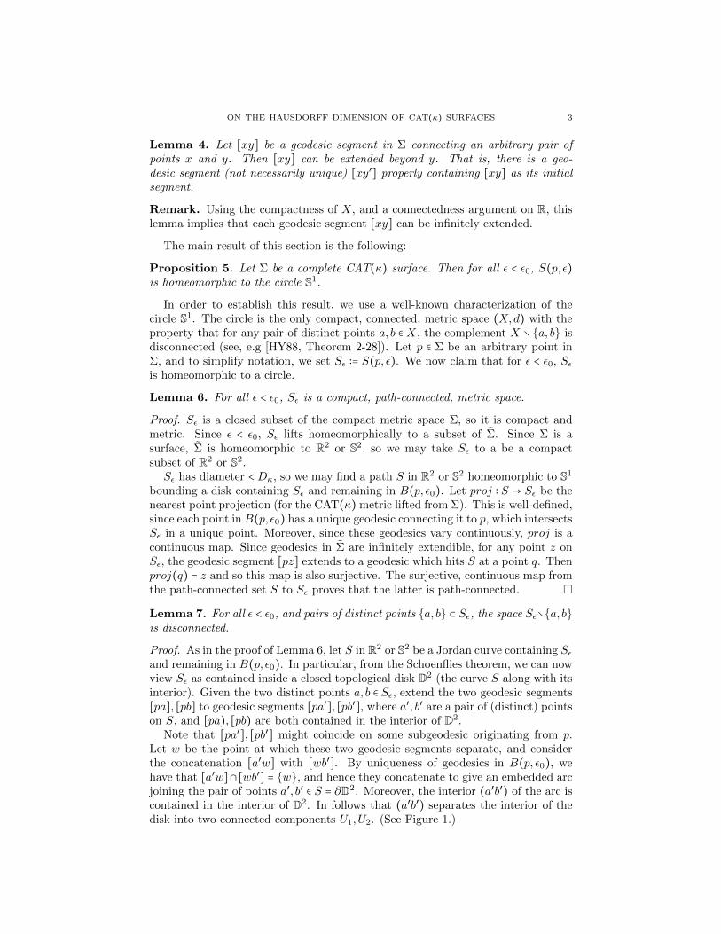
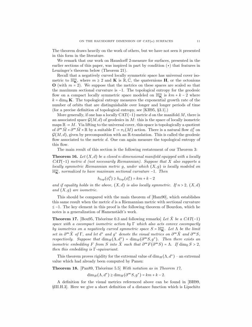
Proof. As in the proof of Lemma 6, let S in R2 or S2 be a Jordan curve containing Sεand remaining in B(p, ε0). In particular, from the Schoenflies theorem, we can nowview Sε as contained inside a closed topological disk D2 (the curve S along with itsinterior). Given the two distinct points a, b ∈ Sε, extend the two geodesic segments[pa], [pb] to geodesic segments [pa′], [pb′], where a′, b′ are a pair of (distinct) pointson S, and [pa), [pb) are both contained in the interior of D2.

Note that [pa′], [pb′] might coincide on some subgeodesic originating from p.Let w be the point at which these two geodesic segments separate, and considerthe concatenation [a′w] with [wb′]. By uniqueness of geodesics in B(p, ε0), wehave that [a′w]∩ [wb′] = {w}, and hence they concatenate to give an embedded arcjoining the pair of points a′, b′ ∈ S = ∂D2. Moreover, the interior (a′b′) of the arc iscontained in the interior of D2. In follows that (a′b′) separates the interior of thedisk into two connected components U1, U2. (See Figure 1.)


rr

p

w

Sε

AAAAAAAAAAAAAAAAAAAA

��

r ra b

rra′

b′

S

[a′w] [wb′]U1

U2

Figure 1. Proving Sε is a circle.

Now by way of contradiction, let us assume Sε∖{a, b} is connected. Then withoutloss of generality, Sε ∩U1 must be empty. On the other hand, U1 is homeomorphicto an open disk, whose boundary is a Jordan curve (formed by the arc (a′b′) inthe interior of D2, along with the portion of the boundary S joining a′ to b′). Theboundary of U1 contains the arc (wa′) passing through a, and the distance to pvaries continuously along (wa′) from a number < ε (since w ≠ a) to a number > ε(since a ≠ a′). Pick an arc η inside U1 joining w to a′, and consider the distancefunction restricted to η. It varies continuously from < ε to > ε, but since Sε∩U1 = ∅,is never equal to ε. This is a contradiction, completing the proof. �

Using the topological characterization of S1, Proposition 5 now follows immedi-ately from Lemma 6 and Lemma 7.

3. The geometry of small distance spheres

We now want to find a 0 < δ0 < ε0 such that, for all p ∈ Σ and ε < δ0, Sε isrectifiable with length uniformly bounded above. Let us denote by l(γ) the lengthof a curve γ, where l takes the value ∞ if the curve is not rectifiable.

Lemma 8. Let Σ be a CAT(κ) surface. Then for each p ∈ Σ there exists some0 < ε < ε0 such that S(p, ε) is a rectifiable curve.

Proof. Fix p. By Proposition 5, for ε < ε0, Sε is homeomorphic to a circle. By wayof contradiction, let us assume that for all n ∈ N, Sε/n is not rectifiable, i.e. thatl(Sε/n) =∞.


Note that if ε′′ < ε′ < ε0, the rectifiability of Sε′ implies that Sε′′ is also rectifiable.This follows from the fact that the nearest-point projection πZ to a complete, convexsubset Z is distance non-increasing in a ball of radius < ε0 in a CAT(κ) space (see,e.g. [BH99, Prop. II.2.4 (or the exercise following for κ > 0)]). Applying this to thecomplete convex subset Z ∶= B(p, ε′′), and using the (global) CAT(κ) geometry inB(p, ε0), we see that πZ is just the radial projection towards p. In particular theimage of πZ lies on Sε′′ , showing that l(Sε′′) ≤ l(Sε′) <∞.

r

r

r

p

S(1)

N(1)

&%'$

Sε/n

Sε

arcW (1) arcE(1)

arcE(n)

rr

N(n)

S(n)

��r

��

��

��

rz∗

q[z∗q]

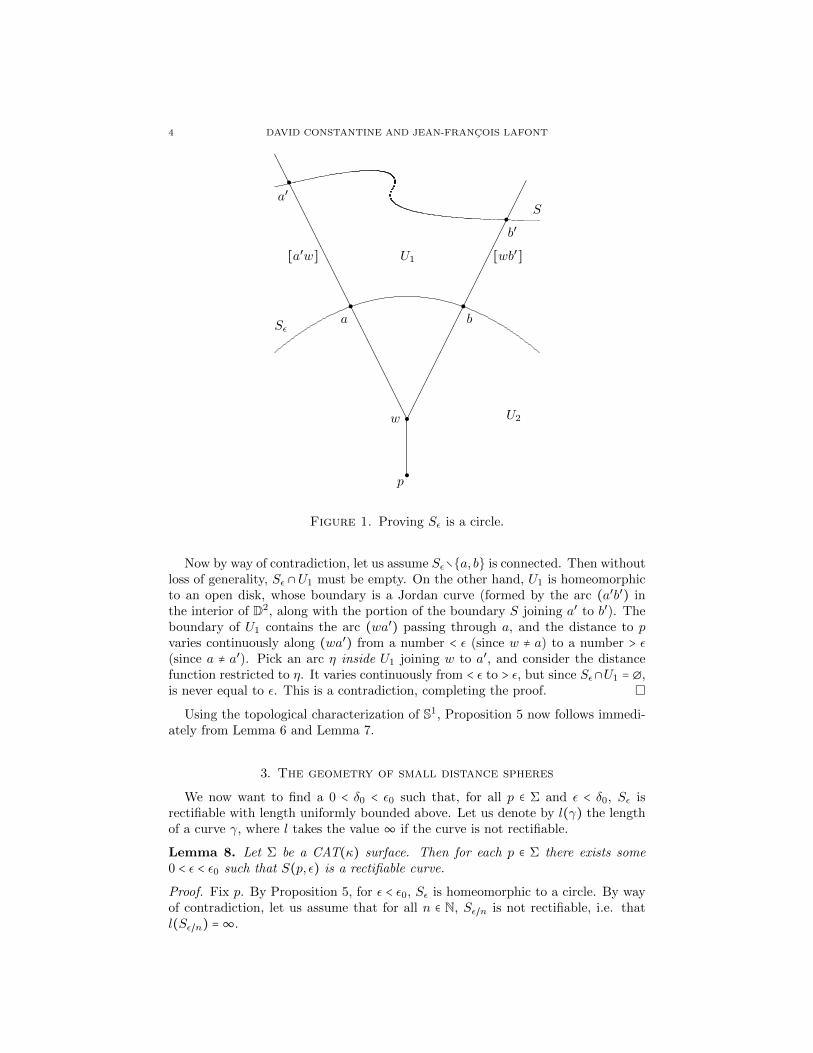
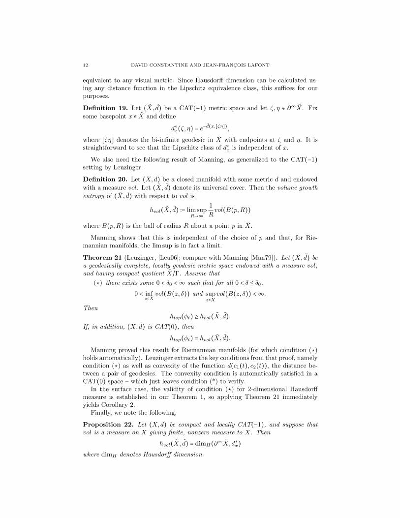
Figure 2. A geodesic configuration which cannot occur if Sε/n isnot rectifiable.

Fix any geodesic γ through p and denote by N(n) and S(n) its two intersec-tions with Sε/n (chosen so that all N(n) lie on the same component of γ ∖ {p}).Since Sε/n is a circle, the pair {N(n), S(n)} divides Sε/n into two arcs, whose clo-sures we call arcE(n) and arcW (n); choose these so that the relative positionsof N(n), S(n), arcE(n) and arcW (n) correspond to the cardinal directions on acompass.

Note that for all n, at least one of l(arcE(n)), l(arcW (n)) must be infinite, sincel(Sε/n) is infinite. Without loss of generality, we may assume that l(arcE(n)) =∞for infinitely many n, and hence (by the discussion above) for all n. We focus ourattention now on the family {arcE(n)}n∈N.

On arcE(1) define the following equivalence relation: we declare x ∼ y if thereexists some n such that the arc in arcE(n) with endpoints [px] ∩ arcE(n) and[py] ∩ arcE(n) is of finite length. That this is an equivalence relation is easy tocheck. We denote equivalence classes by [x].

We note two things about arcE(1)/ ∼ and its equivalence classes. First, N(1) ≁S(1), for otherwise arcE(n) would have finite length for some n. Second, for eachx ∈ arcE(1), [x] is an interval (possibly degenerate). This is because geodesics areunique at the scale we work at, and if three points are arranged around arcE(1)in order x < y < z, then [px] ∩ arcE(n) ≤ [py] ∩ arcE(n) ≤ [pz] ∩ arcE(n). Here we


use <,≤ to denote the ordering of points as they occur along the path arcE(n) fromN(n) to S(n). Thus the decomposition of arcE(1) into the equivalence classes of∼ is a decomposition into at least two disjoint subintervals (possibly degenerate) ofthe half-circle arcE(1).

By connectedness of arcE(1), either [N(1)] or [S(1)] is a singleton, or someequivalence class has a closed endpoint in the interior of arcE(1). Let z∗ be thisendpoint or the singleton N(1) or S(1).

If z∗ is an endpoint of arcE(1), let q be any other point in arcE(1). If z∗ is theclosed endpoint of [z∗] in the interior of arcE(1), let q be any point in arcE(1)which lies on the z∗-side of [z∗]. We note that there are infinitely many such q,and by the choice of z∗ and the topology of the half-circle arcE(1), we may take asequence of such q approaching z∗. Observe that, since q and z∗ are not equivalent,the geodesic segments [pz∗] and [pq] only agree at the point p.

Consider the geodesic segment [z∗q]. By the properties of geodesics in the(globally) CAT(κ) set B(p, ε), this geodesic segment lies inside B(p, ε) and doesnot cross the geodesic γ which divides the West and East parts of B(p, ε). Supposethat [z∗q] does not intersect arcE(n) for some n (as in Figure 2). Then the radialprojection of [z∗q] onto Sn provides a path in arcE(n) from [pz∗] ∩ arcE(n) to[pq] ∩ arcE(n). Again by the distance non-increasing properties of the projection,since [z∗q] has finite length, this would imply z∗ ∼ q, which contradicts the choiceof q. Therefore the geodesic segment [z∗q] must intersect arcE(n) for all n. It musttherefore hit p, and by uniqueness of geodesics we conclude that [z∗q] = [z∗p]∪[pq].

Now consider B(z∗, ε). The work above shows that no q chosen as previouslydescribed lies in B(z∗, ε). But this contradicts our observation above that, usingthe half-circle topology of arcE(1), we may take such q approaching z∗. Thiscontradiction implies that for some n, Sε/n must be rectifiable, concluding theproof. �

Using the compactness of Σ, we can now promote the pointwise result in Lemma8 to a global result:

Lemma 9. Let Σ be a closed CAT(κ) surface. Then there exist δ0 > 0 and someuniform C > 0 such that for all p ∈ Σ, l(S(p, δ0)) < C.

Proof. Suppose there is no finite, uniform bound on l(S(p, δ0)), for any δ0. Thenwe may take a sequence of points pn in Σ with l(S(pn,1/n)) ≥ n. Let p∗ beany subsequential limit point of (pn). We know by Lemma 8 that there existssome ε > 0 such that l(S(p∗, ε)) < ∞. For n sufficiently large, B(p∗, ε) properlycontains S(pn,1/n). But then the unbounded lengths of the latter, plus againthe distance non-increasing properties of nearest-point projection, applied to theprojection from S(p∗, ε) to B(pn,1/n), would imply that the length of S(p∗, ε) isinfinite, contradicting Lemma 8. This proves the Lemma. �

4. Proof of Theorem 1

We define a particular non-expanding map from B(p, ε0) to the ball of radius ε0in the model space H2. This will be a key tool in our proof of Theorem 1.

Define an equivalence relation on the set of geodesic segments starting at p bydeclaring γ1 ∼ γ2 if the Alexandrov angle between these segments at p is 0.


Definition 10. (See, e.g. [BH99, Definition II.3.18]) The set of equivalence classesfor ∼, equipped with the metric provided by the Alexandrov angle, is the space ofdirections at p, denoted Sp(Σ).

The following result is standard:

Proposition 11. (See, e.g. [BH99, Theorem II.3.19]) If Σ is CAT(κ) for any κ,

then for each p ∈ Σ, the completion of Sp(Σ) is CAT(1).

Lemma 12. For any p ∈ Σ, where Σ is a CAT(κ) surface, Sp(Σ) ≅ S1.

Proof. The natural projection from Sε to Sp(Σ) is continuous and, by Lemma 4,

surjective. The fiber over any point in Sp(Σ) is easily seen to be a closed interval.

Thus Sp(Σ) is homeomorphic to a quotient of S1, where each equivalence classis a closed interval in S1. It is a well-known result that such a quotient space isautomatically homeomorphic to S1 (this can be easily shown using the topologicalcharacterization of S1 used in the proof of Proposition 5). This establishes theLemma. �

Combining Proposition 11 with Lemma 12, which implies that Sp(Σ) is complete,we have

Corollary 13. For any p ∈ Σ, Sp(Σ) is CAT(1).

We now construct the non-expanding map to the model surface Mκ of con-stant curvature κ. We closely follow the proof of a similar result presented in[BBI01, Proposition 10.6.10], but for the opposite type of curvature bound (curva-ture bounded below, rather than above).

Proposition 14. Let Σ be a CAT(κ) surface and p any point in Σ. Let ε0 be asabove. Then there is a map f ∶ B(p, ε0)→Mκ such that

(1) dMκ(f(x), f(y)) ≤ dΣ(x, y) for all x, y ∈ B(p, ε0),(2) dMκ(f(p), f(y)) = dΣ(p, y) for all y ∈ B(p, ε0), and(3) f(B(p, ε)) = BMκ(f(p), ε).

Proof. By the choice of ε0, we can work in Σ or lift B(p, ε0) homeomorphically to

Σ. By corollary 13, Sp(Σ) is CAT(1). It is homeomorphic to S1, so it is easy to

see that there is a surjective map g ∶ Sp(Σ)→ S1 which is non-expanding:

dS1(g(v), g(w)) ≤∡p(v,w) for all v,w ∈ Sp(Σ).

Let Kκp (Σ) denote the κ-cone over Sp(Σ). This space is topologically a cone over

Sp(Σ) with origin denoted o and coordinates (v, r) away from o, where v ∈ Sp(Σ)and r > 0 (with r truncated at π/

√κ if κ > 0). It is equipped with a metric devised

so that the κ-cone over the circle is the model space of curvature κ. For details ofits construction see, e.g., [BBI01, §10.2.1]. Its key property for our purposes is the

following: since Sp(Σ) is CAT(1), Kκp (Σ) is CAT(κ) ([BH99, Theorem II.3.14]).

On the ball B(p, ε0) define a logarithm map as follows:

logp ∶ B(p, ε0)→Kκp (Σ)

p↦ o

x ≠ p↦ (v, dΣ(p, x))


where v is the direction in Sp(Σ) of the geodesic segment [px]. From the non-

expanding property of g and the definition of Kκp (Σ),

dKκp (Σ)

(logp(x), logp(y)) ≤ dΣ(x, y) for all x, y ∈ B(p, ε0).

By its definition, logp preserves distance from the origin, and by its definition, logpmaps B(p, ε) surjectively onto BK−1

p (Σ)(o, ε).

Again, using the definition of Kκp (Σ), the non-expanding map g ∶ Sp(Σ) → S1

extends to a map G ∶ Kκp (Σ) → Mκ, obtained by realizing Mκ as the κ-cone over

S1. The map is non-expanding since g is, and preserves distance from the origin.G sends BKκ

p (Σ)(o, ε) surjectively to BMκ(G(o), ε) because g is surjective. Then

f = G ○ logp is the desired map. �

We are now ready to prove Theorem 1.

Proof of Theorem 1. Let δ0 < ε0 be given by Lemma 9 and let δ < δ0. First webound H2(B(p, δ)) below. Recall that the Hausdorff 2-measure of some metricspace X is defined via a two step process. For some ρ > 0, one considers opencovers {Ui} of X by open sets of diameter < ρ, and takes the infimum of ∑diamU2

i

over all such covers. This defines the quantity H2ρ(X), which is non-increasing as a

function of ρ. The Hausdorff 2-measure is then the supremum of the H2ρ(X) (which

of course coincides with the limit of these as ρ→ 0).Let f be the non-expanding map provided by Proposition 14. Since f preserves

radial distance from the origin, f(B(p, δ)) ⊆ B(f(p), δ). Fix any ρ > 0 and sup-pose {Ui} is a countable cover of B(p, δ) with diam(Ui) < ρ. Then the collection{f(Ui)} covers B(f(p), δ) and diam(f(Ui)) ≤ diam(Ui) < ρ as f is non-expanding.Therefore,

Σi diamUi2 ≥ Σi diam f(Ui)2 ≥H2

ρ(B(f(p), δ)).

Passing to the infimum over all such covers {Ui} of B(p, δ), we obtain for eachρ > 0 the inequality H2

ρ(B(p, δ)) ≥ H2ρ(B(f(p), δ)). Passing to the limit as ρ → 0,

this gives H2(B(p, δ)) ≥H2(B(f(p), δ)). Finally, one observes that the right handside H2(B(f(p), δ)) is just the volume of a δ ball in the model space Mκ. Sincethis quantity is independent of the choice of point p, this gives the desired uniformlower bound on H2(B(p, δ)).

Now we bound H2(B(p, δ)) above. This portion of the proof uses the uni-form bound on the length of Sδ obtained in Lemma 9. It is sufficient to boundH2(B(p, δ0)) uniformly above.

Fix ρ < δ0. Let Eρ be any minimal cardinality subset of Sδ0 which is ρ2-dense

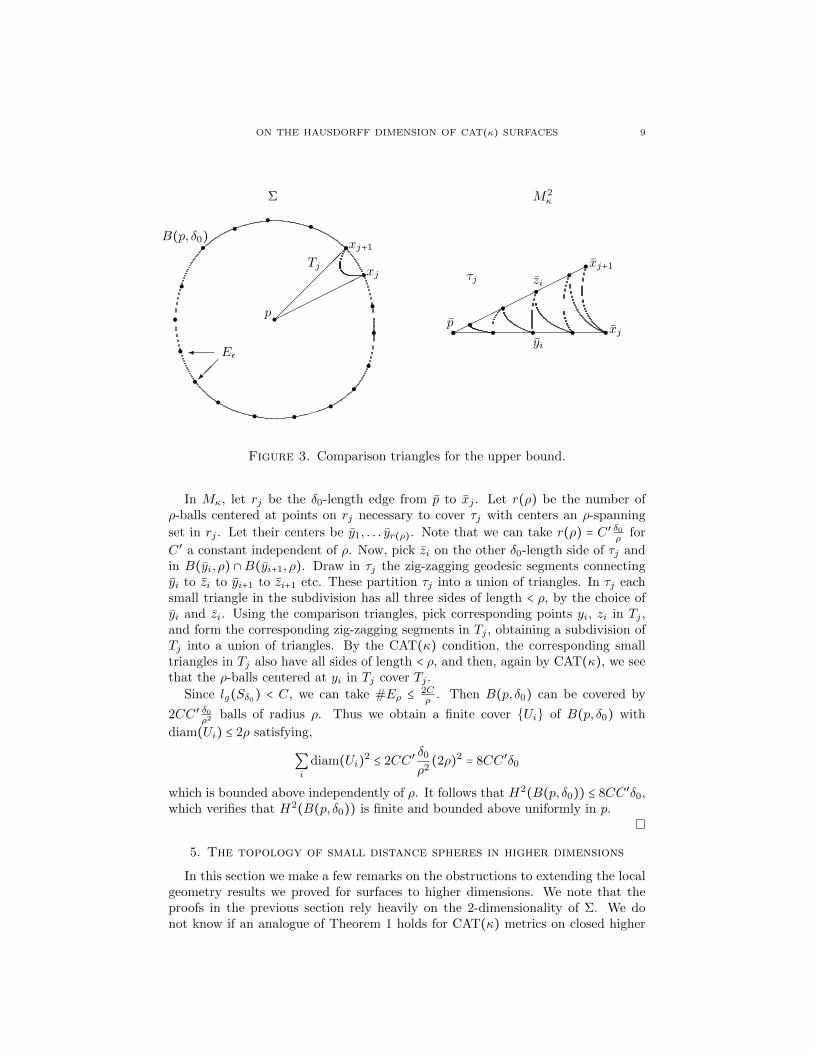
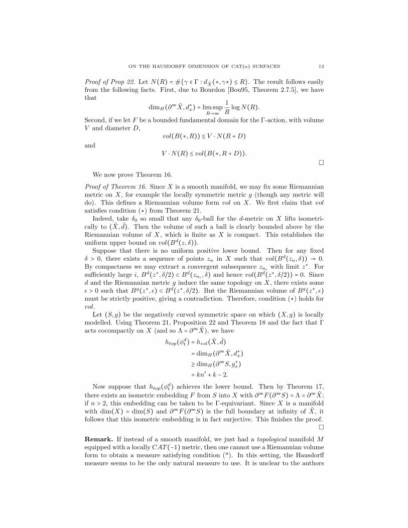
inside Sδ0 . The circumference bound allows us to uniformly bound #Eρ. Indexxj ∈ Eρ in order around Sδ0 . Let Tj be the geodesic triangle with vertices p, xj , xj+1.Tj has edges of length δ0, δ0 and < ρ. Let τj be the corresponding comparisontriangle in Mκ (see Figure 3).


Σ M2κ

B(p, δ0)

rp��

��

��

rrrrrrrrrrr

rrr

r r r rxj+1

xjTj

rr

rr r r rr r r r

yi

zi

p

xj+1

xj

τj

��

��

�

Eε��

�

Figure 3. Comparison triangles for the upper bound.

In Mκ, let rj be the δ0-length edge from p to xj . Let r(ρ) be the number ofρ-balls centered at points on rj necessary to cover τj with centers an ρ-spanning

set in rj . Let their centers be y1, . . . yr(ρ). Note that we can take r(ρ) = C ′ δ0ρ

for

C ′ a constant independent of ρ. Now, pick zi on the other δ0-length side of τj andin B(yi, ρ) ∩B(yi+1, ρ). Draw in τj the zig-zagging geodesic segments connectingyi to zi to yi+1 to zi+1 etc. These partition τj into a union of triangles. In τj eachsmall triangle in the subdivision has all three sides of length < ρ, by the choice ofyi and zi. Using the comparison triangles, pick corresponding points yi, zi in Tj ,and form the corresponding zig-zagging segments in Tj , obtaining a subdivision ofTj into a union of triangles. By the CAT(κ) condition, the corresponding smalltriangles in Tj also have all sides of length < ρ, and then, again by CAT(κ), we seethat the ρ-balls centered at yi in Tj cover Tj .

Since lg(Sδ0) < C, we can take #Eρ ≤ 2Cρ

. Then B(p, δ0) can be covered by

2CC ′ δ0ρ2

balls of radius ρ. Thus we obtain a finite cover {Ui} of B(p, δ0) with

diam(Ui) ≤ 2ρ satisfying,

∑i

diam(Ui)2 ≤ 2CC ′ δ0ρ2

(2ρ)2 = 8CC ′δ0

which is bounded above independently of ρ. It follows that H2(B(p, δ0)) ≤ 8CC ′δ0,which verifies that H2(B(p, δ0)) is finite and bounded above uniformly in p.

�

5. The topology of small distance spheres in higher dimensions

In this section we make a few remarks on the obstructions to extending the localgeometry results we proved for surfaces to higher dimensions. We note that theproofs in the previous section rely heavily on the 2-dimensionality of Σ. We donot know if an analogue of Theorem 1 holds for CAT(κ) metrics on closed higher


dimensional manifolds. One of the first steps in our proof was Proposition 5, whichshowed that the small enough metric spheres inside locally CAT(κ) surfaces werehomeomorphic to the circle S1. The analogous statement fails in dimensions ≥ 5,as the well-known example below shows.

Proposition 15 (Davis-Januszkiewicz). For each dimension n ≥ 5, there exists aclosed n-manifold M equipped with a piecewise hyperbolic, locally CAT(−1) metric,and a point p ∈ M with the property that for all small enough ε, the ε-sphere Sεcentered at p is not homeomorphic to Sn−1. In fact, Sε is not even a manifold.

Proof. Such examples can be found in the work of Davis and Januszkiewicz [DJ91,Theorem 5b.1]. We briefly summarize the construction for the convenience of thereader. Start with a closed smooth homology sphere Nn−2 which is not homeomor-phic to Sn−2. Such manifolds exist for all n ≥ 5, and are quotients of Sn−2 by asuitable perfect group π1(Nn−2). Take a smooth triangulation of Nn−2, and con-sider the induced triangulation T on the double suspension Σ2(Nn−2). By workof Cannon and Edwards [Can79, Edw], Σ2(Nn−2) is homeomorphic to Sn. Thetriangulation T on Sn is not a PL-triangulation, as there exists a 4-cycle in the 1-skeleton of the triangulation whose link is homeomorphic to Nn−2. Now apply thestrict hyperbolization procedure of Charney and Davis [CD95] to the triangulatedmanifold (Sn,T ).

This outputs a piecewise-hyperbolic, locally CAT(-1) space M . A key point ofthe hyperbolization procedure is that it preserves the local structure. Since theinput (Sn,T ) is a closed n-manifold, the output M is also a closed n-manifold.The 4-cycle in T whose link was homeomorphic to Nn−2 now produces a closedgeodesic γ in M , whose link is still homeomorphic to Nn−2 (i.e. the “unit normal”to γ forms a copy of Nn−2). It follows from this that, picking the point p on γ, allsmall ε-spheres Sε are homeomorphic to the suspension ΣNn−2. Since Nn−2 wasnot the standard sphere, Sε ≅ ΣNn−2 fails to be a manifold at the suspension pointx, as every small punctured neighborhood of x will have non-trivial π1. We referthe reader to [DJ91, Section 5] for more details.

�

This cautionary example suggests that small metric spheres in high-dimensionallocally CAT(κ) manifolds could exhibit pathologies. In view of these results, andthe interest in obtaining higher dimensional analogs, we raise the following question.

Question . Let M be a closed n-manifold equipped with a locally CAT(−1) metricof Hausdorff dimension d. Can d ever be strictly larger than n? Do the uniformbound conditions of Theorem 1 hold in higher dimensions?

The authors suspect that examples with d > n do indeed exist in higher dimen-sions.

6. Entropy rigidity in CAT(-1)

In this section we present an entropy rigidity result for closed CAT(−1) mani-folds. This result generalizes Hamenstadt’s entropy rigidity result from [Ham90] tothe CAT (−1) setting. It is very closely related to, and in fact relies on, a rigid-ity result of Bourdon. The main addition to Bourdon’s theorem is the connectionto topological entropy via a theorem of Leuzinger (generalizing work of Manning).


The theorem draws heavily on the work of others, but we have not seen it presentedin this form in the literature.

We remark that our work on Hausdorff 2-measure for surfaces, presented in theearlier sections of this paper, was inspired in part by condition (⋆) that features inLeuzinger’s theorem below (Theorem 21).

Recall that a negatively curved locally symmetric space has universal cover iso-metric to HmK, where m ≥ 2 and K is R,C, the quaternions H, or the octonionsO (with m = 2). We suppose that the metrics on these spaces are scaled so thatthe maximum sectional curvature is −1. The topological entropy for the geodesicflow on a compact locally symmetric space modeled on HmK is km + k − 2 wherek = dimR K. The topological entropy measures the exponential growth rate of thenumber of orbits that are distinguishable over longer and longer periods of time(for a precise definition of topological entropy, see [KH95, §3.1].)

More generally, if one has a locally CAT(−1) metric d on the manifold M , there isan associated space G(M,d) of geodesics in M : this is the space of locally isometricmaps R→M . Via lifting to the universal cover, this space is topologically a quotientof ∂∞M × ∂∞M ×R by a suitable Γ ∶= π1(M) action. There is a natural flow φdt onG(M,d), given by precomposition with an R-translation. This is called the geodesicflow associated to the metric d. One can again measure the topological entropy ofthis flow.

The main result of this section is the following restatement of our Theorem 3:

Theorem 16. Let (X,d) be a closed n-dimensional manifold equipped with a locallyCAT(−1) metric d (not necessarily Riemannian). Suppose that X also supports alocally symmetric Riemannian metric g, under which (X,g) is locally modeled onHmK, normalized to have maximum sectional curvature −1. Then

htop(φdt ) ≥ htop(φgt ) = km + k − 2

and if equality holds in the above, (X,d) is also locally symmetric. If n > 2, (X,d)and (X,g) are isometric.

This should be compared with the main theorem of [Ham90], which establishesthis same result when the metric d is a Riemannian metric with sectional curvature≤ −1. The key element in this proof is the following theorem of Bourdon, which henotes is a generalization of Hamenstadt’s work.

Theorem 17. [Bou95, Theoreme 0.3 and following remarks] Let X be a CAT(−1)space with a cocompact isometric action by Γ which also acts convex cocompactlyby isometries on a negatively curved symmetric space S = HmK. Let Λ be the limit

set in ∂∞X of Γ, and let d∗ and g∗ denote the visual metrics on ∂∞X and ∂∞S,respectively. Suppose that dimH(Λ, d∗) = dimH(∂∞S, g∗). Then there exists an

isometric embedding F from S into X such that ∂∞F (∂∞S) = Λ. If dimR S > 2,then this embedding is Γ-equivariant.

This theorem proves rigidity for the extremal value of dimH(Λ, d∗) – an extremalvalue which had already been computed by Pansu:

Theorem 18. [Pan89, Theoreme 5.5] With notation as in Theorem 17,

dimH(Λ, d∗) ≥ dimH(∂∞S, g∗) = km + k − 2.

A definition for the visual metrics referenced above can be found in [BH99,§III.H.3]. Here we give a short definition of a distance function which is Lipschitz


equivalent to any visual metric. Since Hausdorff dimension can be calculated us-ing any distance function in the Lipschitz equivalence class, this suffices for ourpurposes.

Definition 19. Let (X, d) be a CAT(−1) metric space and let ζ, η ∈ ∂∞X. Fix

some basepoint x ∈ X and define

d∗x(ζ, η) = e−d(x,[ζη]),

where [ζη] denotes the bi-infinite geodesic in X with endpoints at ζ and η. It isstraightforward to see that the Lipschitz class of d∗x is independent of x.

We also need the following result of Manning, as generalized to the CAT(−1)setting by Leuzinger.

Definition 20. Let (X,d) be a closed manifold with some metric d and endowed

with a measure vol. Let (X, d) denote its universal cover. Then the volume growth

entropy of (X, d) with respect to vol is

hvol(X, d) ∶= lim supR→∞

1

Rvol(B(p,R))

where B(p,R) is the ball of radius R about a point p in X.

Manning shows that this is independent of the choice of p and that, for Rie-mannian manifolds, the lim sup is in fact a limit.

Theorem 21 (Leuzinger, [Leu06]; compare with Manning [Man79]). Let (X, d) bea geodesically complete, locally geodesic metric space endowed with a measure vol,and having compact quotient X/Γ. Assume that

(⋆) there exists some 0 < δ0 <∞ such that for all 0 < δ ≤ δ0,

0 < infz∈X

vol(B(z, δ)) and supz∈X

vol(B(z, δ)) <∞.

Then

htop(φt) ≥ hvol(X, d).If, in addition, (X, d) is CAT(0), then

htop(φt) = hvol(X, d).

Manning proved this result for Riemannian manifolds (for which condition (⋆)holds automatically). Leuzinger extracts the key conditions from that proof, namelycondition (⋆) as well as convexity of the function d(c1(t), c2(t)), the distance be-tween a pair of geodesics. The convexity condition is automatically satisfied in aCAT(0) space – which just leaves condition (*) to verify.

In the surface case, the validity of condition (⋆) for 2-dimensional Hausdorffmeasure is established in our Theorem 1, so applying Theorem 21 immediatelyyields Corollary 2.

Finally, we note the following.

Proposition 22. Let (X,d) be compact and locally CAT(−1), and suppose thatvol is a measure on X giving finite, nonzero measure to X. Then

hvol(X, d) = dimH(∂∞X, d∗x)where dimH denotes Hausdorff dimension.


Proof of Prop 22. Let N(R) = #{γ ∈ Γ ∶ dX(∗, γ∗) ≤ R}. The result follows easilyfrom the following facts. First, due to Bourdon [Bou95, Theorem 2.7.5], we havethat

dimH(∂∞X, d∗x) = lim supR→∞

1

RlogN(R).

Second, if we let F be a bounded fundamental domain for the Γ-action, with volumeV and diameter D,

vol(B(∗,R)) ≤ V ⋅N(R +D)and

V ⋅N(R) ≤ vol(B(∗,R +D)).�

We now prove Theorem 16.

Proof of Theorem 16. Since X is a smooth manifold, we may fix some Riemannianmetric on X, for example the locally symmetric metric g (though any metric willdo). This defines a Riemannian volume form vol on X. We first claim that volsatisfies condition (⋆) from Theorem 21.

Indeed, take δ0 so small that any δ0-ball for the d-metric on X lifts isometri-cally to (X, d). Then the volume of such a ball is clearly bounded above by theRiemannian volume of X, which is finite as X is compact. This establishes theuniform upper bound on vol(Bd(z, δ)).

Suppose that there is no uniform positive lower bound. Then for any fixedδ > 0, there exists a sequence of points zn in X such that vol(Bd(zn, δ)) → 0.By compactness we may extract a convergent subsequence zni with limit z∗. Forsufficiently large i, Bd(z∗, δ/2) ⊂ Bd(zni , δ) and hence vol(Bd(z∗, δ/2)) = 0. Sinced and the Riemannian metric g induce the same topology on X, there exists someε > 0 such that Bg(z∗, ε) ⊂ Bd(z∗, δ/2). But the Riemannian volume of Bg(z∗, ε)must be strictly positive, giving a contradiction. Therefore, condition (⋆) holds forvol.

Let (S, g) be the negatively curved symmetric space on which (X,g) is locallymodelled. Using Theorem 21, Proposition 22 and Theorem 18 and the fact that Γacts cocompactly on X (and so Λ = ∂∞X), we have

htop(φdt ) = hvol(X, d)

= dimH(∂∞X, d∗x)≥ dimH(∂∞S, g∗x)= kn′ + k − 2.

Now suppose that htop(φdt ) achieves the lower bound. Then by Theorem 17,

there exists an isometric embedding F from S into X with ∂∞F (∂∞S) = Λ = ∂∞X;if n > 2, this embedding can be taken to be Γ-equivariant. Since X is a manifoldwith dim(X) = dim(S) and ∂∞F (∂∞S) is the full boundary at infinity of X, itfollows that this isometric embedding is in fact surjective. This finishes the proof.

�

Remark. If instead of a smooth manifold, we just had a topological manifold Mequipped with a locally CAT (−1) metric, then one cannot use a Riemannian volumeform to obtain a measure satisfying condition (*). In this setting, the Hausdorffmeasure seems to be the only natural measure to use. It is unclear to the authors


whether or not the Hausdorff measure must satisfy the regularity condition (*).Note that Davis and Januszkiewicz [DJ91] give examples, in dimensions n ≥ 5, ofnon-smoothable closed topological manifolds Mn which support locally CAT (−1)metrics.

References

[BBI01] Dmitri Burago, Yuri Burago, and Sergei Ivanov. A course in metric geometry, volume 33

of Graduate Studies in Mathematics. American Mathematical Society, 2001.[BH99] Martin R. Bridson and Andre Haefliger. Metric spaces of non-positive curvature, volume

319 of Grundlehren der mathematischen Wissenschaften. Springer, Berlin, 1999.

[Bou95] M. Bourdon. Structure conforme au bord et flot geodesique d’un CAT(-1)-espace. En-seign. Math., 41(2):63–102, 1995.

[Bou96] Marc Bourdon. Sur le birapport au bord des cat(-1)-espaces. Publications mathematiques

de l’I.H.E.S., 83:95–104, 1996.

[Can79] J.W. Cannon. Shrinking cell-like decompositions of manifolds. codimension three. Annalsof Mathematics, 110(1):83–112, 1979.

[CD95] Ruth M. Charney and Michael Davis. Strict hyperbolization. Topology, 34(2):329–350,

1995.[DJ91] Michael Davis and Tadeusz Januszkiewicz. Hyperbolization of polyhedra. J. Differential

Geometry, 34(2):347–388, 1991.

[Edw] Robert D. Edwards. Suspensions of homology spheres. Available atArXiv:math/0610573.

[Ham90] Ursula Hamenstadt. Entropy-rigidity of locally symmetric spaces of negative curvature.

Annals of Mathematics, 131(1):35–51, 1990.[HY88] John G. Hocking and Gail S. Young. Topology. Dover, New York, 1988.

[KH95] Anatole Katok and Boris Hasselblatt. Introduction to the modern theory of dynamicalsystems. Cambridge University Press, 1995.

[Leu06] Enrico Leuzinger. Entropy of the geodesic flow for metic spaces and Bruhat-Tits build-

ings. Adv. Geom., 6:475–491, 2006.[Man79] Anthony Manning. Topological entropy for geodesic flows. Annals of Mathematics,

110(3):567–573, 1979.

[Pan89] Pierre Pansu. Dimension conforme et sphere a l’infini des varietes a courbure negative.Ann. Acad. Sci. Fenn. Ser. A I Math., 14(2):177–212, 1989.

[TW05] Jeremy T. Tyson and Jang-Mei Wu. Characterizations of snowflake metric spaces. Ann.

Acad. Sci. Fenn. Ser. A I Math., 30(2):313–336, 2005.

Wesleyan University, Mathematics and Computer Science Department, Middletown,CT 06459

Department of Mathematics, Ohio State University, Columbus, Ohio 43210

Documents

ON THE HAUSDORFF DIMENSION OF CAT SURFACES