Hausdorff Dimension, Its Properties, and Its Surprises

Hausdorff Dimension, Its Properties,and Its Surprises

Dierk Schleicher

1. INTRODUCTION. The concept of dimension has many aspects and meaningswithin mathematics, and there are a number of very different definitions of what thedimension of a set should be. The simplest case is that of R

d : in order to distinguishpoints in R

d , we need d different (real) coordinates, so Rd has dimension d as a (real)

vector space. Similarly, a d-dimensional manifold is a space that locally looks like apiece of R

d .Another interesting concept is the topological dimension of a topological space: ev-

ery discrete set has topological dimension 0 (e.g., any finite sets of points in Rd), an

injective curve has topological dimension 1, a disk has dimension 2 and so on. Theidea is that a set of dimension d can be disconnected in a neighborhood of every pointby a set of dimension d − 1: curves and circles can be disconnected by removing iso-lated points, disks can be disconnected by removing curves and circles, etc. A formaldefinition is recursive, starting conveniently with the empty set: the empty set has topo-logical dimension −1, and a set has topological dimension at most d if each point hasa basis of open neighborhoods whose boundaries have topological dimension at mostd − 1.

All these dimensions, if finite, are integers (we will ignore infinite-dimensionalspaces). An interesting discussion of various concepts of dimension, different in spiritfrom ours, can be found in the recent article of Manin [17].

We will be concerned with a different aspect of dimension, having to do with self-similarity of “fractal” sets such as those shown in Figure 1. As Mandelbrot pointsout [16, p. 1], “clouds are not spheres, mountains are not cones, coastlines are notcircles, and bark is not smooth, nor does lightning travel in a straight line,” so manyobjects occurring in nature are not manifolds. For instance, the fern in Figure 1 isconstructed by a simple affine self-similarity process, and people have tried to describethe hairy systems of roots of trees or plants in terms of “fractals”, rather than as smoothmanifolds. Similar remarks apply to the human lung or to the borders of most statesand countries.

The concept of Hausdorff dimension is almost a century old, but it has receivedparticularly prominent attention since the advent of computer graphics and the com-puter power to simulate and visualize beautiful objects with importance in a numberof sciences. Earlier, such sets were often constructed by ad hoc methods as coun-terexamples to intuitive conjectures. In the first part of this paper, we try to convinceinterested readers that Hausdorff dimension is the “right” concept to describe interest-ing properties of a metric set X : for each number d in R

+0 we define the d-dimensional

Hausdorff measure μd(X); if d is a positive integer and X = Rd , then this measure

coincides with Lebesgue measure (up to a normalization factor). There is a thresholdvalue for d, called dimH (X), such that μd(X) = 0 if d > dimH (X) and μd(X) = ∞if d < dimH (X). This value dimH (X) is the Hausdorff dimension of X .

We first help to develop intuition for this natural concept, and then we challenge itby describing a number of relatively newly discovered sets with very remarkable andsurprising (possibly counterintuitive!) properties of Hausdorff dimension. To describe

June–July 2007] HAUSDORFF DIMENSION 509

(a)

(b)

(c)

(d) (e)

Figure 1. Several “fractal” subsets of R2: (a) the “snowflake” (von Koch) curve: each of its three (fractal) sidescan be disassembled into four pieces, each of which is a copy of the entire side, shrunk by a factor 1/3; (b) theCantor middle-third set, consisting of two copies of itself, shrunk by 1/3; (c) a “fractal” square in the plane,consisting of four shrunk copies of itself with a factor 1/3 (so it has the same dimension as the snowflake!);(d) a fern; (e) the Julia set of a quadratic polynomial.

510 c© THE MATHEMATICAL ASSOCIATION OF AMERICA [Monthly 114

such sets, imagine a curve γ : (0, ∞) → C that connects the point 0 to ∞ (we identifya curve γ : I → C with its image set {γ (t): t ∈ I } in C). Curves have dimension atleast 1, possibly more, but the two endpoints certainly have dimension 0. Now take acollection of disjoint curves γh , each connecting a different point zh to ∞. For example,let zh = ih for h in [0, 1] and γh(t) = ih + γ (t) (provided γ is such that all γh aredisjoint). Then the endpoints are an interval with dimension 1, while the union of allcurves γh covers an open set of C and should certainly have dimension 2. This is trueand intuitive: the union of the endpoints has smaller dimension than the union of thecurves. In this paper, we describe the following situation [24]:

Theorem 1 (A Hausdorff Dimension Paradox). There are subsets E and R of C

with the following properties:

(1) E and R are disjoint;(2) each path component of R is an injective curve (a “ray”) γ : (0, ∞) → C con-

necting some point e of E to ∞ (i.e., limt→0 γ (t) = e and limt→∞ γ (t) = ∞);(3) each point e of E is the endpoint of one or several curves in R;(4) the set R = ⋃

γ ((0, 1)) of rays has Hausdorff dimension 1;(5) the set E of endpoints has Hausdorff dimension 2 and even full 2-dimensional

Lebesgue measure (i.e., the set C \ E has measure zero);(6) stronger yet, we have E ∪ R = C: the set of endpoints E is the complement

of the 1-dimensional set R, yet each point in E is connected to ∞ by one orseveral curves in R!

Mathematics is full of surprising phenomena, and often very artful methods areused to construct sets that exhibit these phenomena. This result is another illustrationthat many of these phenomena arise quite naturally in dynamical systems, especiallycomplex dynamics. It comes at the end of a series of successively stronger results. Thestory started with a surprising result by Karpinska [13]: she established the existenceof natural sets E and R arising in the dynamics of complex exponential maps z �→ λez

for certain values of λ, where E and R enjoy properties (1)–(4), as well as (5) in theform that E has Hausdorff dimension 2. In [26], this result was extended to exponentialmaps with λ in C

∗ = C \ {0} arbitrary. In [23], this was carried over to maps of theform z �→ aez + be−z; in this case, E always has positive 2-dimensional Lebesguemeasure. Finally, condition (6) was established for maps like z �→ π sinh z [24].

We start this paper with a discussion of several concepts of dimension (section 2).In section 3, we give the definition of Hausdorff dimension together with a number ofits fundamental properties. In section 4, we describe a beautiful example constructedby Bogusława Karpinska in which E has positive 2-dimensional Lebesgue measure.In the remainder of the paper, we show that sets E and R satisfying all the assertionsof Theorem 1, including C = E ∪ R, appear naturally in complex dynamics, wheniterating maps such as z �→ π sin z.

The basic features of iterated complex sin and sinh maps are described in section 5,and a fundamental lemma for estimating Hausdorff dimension is given in section 6. Insection 7, we then describe the dynamics of the map z �→ π sin z in detail and finishthe proof of Theorem 1. Finally, we discuss some related known results about planarLebesgue measure, including a theorem of McMullen and a conjecture of Milnor.

The purpose of this paper is to highlight interesting phenomena that are observed atthe interface between dimension theory and transcendental dynamics. It cannot serveas an exhaustive survey on the exciting work that has been done on these two areas,and we can mention only a few of the most interesting references. A good survey of


transcendental dynamics is found in Bergweiler [2]; some more surprising propertiesof exponential dynamics are described in Devaney [4]. The topic of “curves of escapingpoints in transcendental dynamics” was first raised in 1926 by Fatou [10] and taken upmore systematically by Eremenko [8]. In the special case of exponential dynamics, itwas first investigated by Devaney and coauthors [5], [6] and completed in [26], [11].In more general settings, there are existence results in [7], and the current state of theart can be found in the recent thesis of Rottenfußer [22], [21]. Among current work onHausdorff dimension in transcendental dynamics, we would like to mention the surveypapers by Stallard [29] and by Kotus and Urbanski [14]. The results in the current paperhave been extended to larger classes of entire functions in [25]. We apologize to thosewhose work we have not mentioned here.

2. CONCEPTS OF “FRACTAL” DIMENSION. The fundamental idea that leadsto “fractal” dimensions is to investigate interesting sets at different scales of size. Con-sider a regular three-dimensional cube, say of side-length 1. We can subdivide thiscube into many small cubes of side-length s = 1/k for any positive integer k. Obvi-ously, the number of little cubes we obtain is N (s) = k3 = s−3. However, if we sub-divide a unit square into small squares of side-length 1/k, we obtain N (s) = s−2 littlesquares. The exponent here is the dimension: if a set X in R

n can be subdivided intosome finite number N (s) of subsets, all congruent (by translations or rotations) to oneanother and each a rescaled copy of X by a linear factor s, then the “self-similaritydimension” of X is the unique value d that satisfies N (s) = s−d , i.e.,

d = log(N (s))/ log(1/s).

This simple idea can be applied to a number of interesting sets. Consider, forexample, the “snowflake” curve of Figure 1a: we only look at the top third of thesnowflake, above the triangle that we have inscribed for easier description. The detailabove the snowflake shows that this top third can be disassembled into N = 4 pieces,each of which is a rescaled version of the entire top third with a rescaling factor s =1/3. The associated dimension must satisfy 3d = 4 (i.e., d = log 4/ log 3 ≈ 1.26 . . .).The snowflake is a curve (and thus has topological dimension 1), but its self-similaritydimension is greater than that of a straight line: when subdividing a straight line intopieces of one-third the original size, we obtain three pieces; for the snowflake, we getfour (and for a square we get nine). Continued refinement has the same dimension: wecan break up the four pieces into four pieces each, so that all are rescaled by a factors = 1/9; and again d = log(42)/ log(32) = 1.26 . . . .

Let us explore this idea for the standard middle-third Cantor set as shown in Fig-ure 1b. It is constructed by starting with a unit interval, removing the (open) middlethird, so as to yield two closed intervals of length 1/3 each; removing the middle thirdfrom these and continuing inductively yields the standard middle-third Cantor set. Thisset consists of N = 2 parts (left and right) that both are rescaled versions of the orig-inal set with a factor s = 1/3. This Cantor set has dimension log 2/ log 3 ≈ 0.63 . . .:less than a curve, but more than a discrete set of points.

Here is one last example, depicted in Figure 1c: a unit square is subdivided intonine equal subsquares of size s = 1/3, and only the N = 4 subsquares at the verticesare kept and further subdivided. The dimension is log 4/ log 3 ≈ 1.26 . . . as for thesnowflake curve. This set is simply the Cartesian product of the middle-third Cantorset with itself.

We can play with the dimension of the Cantor set. For instance, we can start with aunit interval and remove a shorter or longer interval in the middle so as to leave N = 2


intervals of arbitrary length s in (0, 1/2). In the next generations, we always removean interval in the middle with the same fraction of length, so that the resulting Cantorset is self-similar again. Its dimension is d = log 2/ log(1/s), and it can assume anyreal value in (0, 1).

What we have exploited so far is linear self-similarity of our sets: they consist ofa finite number of pieces, each a linearly rescaled version of the entire set. It is onlyfor such sets that the self-similarity dimension applies. Later, we define two furtherconcepts of “fractal” dimension, box-counting dimension and Hausdorff dimension,which make sense for more general sets than the self-similarity dimension; but for theexamples we have considered so far, all three dimensions apply and have the samevalue.

Here is a variation of the construction that leaves the realm of linearly self-similarsets: take the unit interval, replace it with two subintervals of length s1 ∈ (0, 1/2);each of these two intervals is replaced with two further subintervals of length s1s2

(with s2 in (0, 1/2)), and so on. If all scaling factors si are the same, we have a self-similar Cantor set of dimension d = log 2/ log(1/si) as earlier. If the first k scalingfactors are arbitrary, but sk+1 = sk+2 = · · · = s, then our Cantor set consists of 2k smallCantor sets, and these small Cantor sets are linearly self-similar and have dimensionlog 2/ log(1/s). If the sequence si is not eventually constant, we need a more generalconcept of dimension. We would expect that the dimension would be 0 if si → 0 and1 if si → 1/2. This will be true for the box-counting dimension that we define at theend of this section.

We can even construct a Cantor set within [0, 1] that has positive 1-dimensionalLebesgue measure, so its dimension should certainly be 1: in the first step, weremove the middle interval of length 1/10, say; from the remaining two inter-vals, we remove the central intervals of length 1/200; then we remove four inter-vals of length 1/4000, etc. As a result, the total length of all removed intervals is1/10 + 2/200 + 4/4000 + · · · = 0.1111 . . . = 1/9, so the Cantor set left at the endof the process has 1-dimensional Lebesgue measure 8/9 (note that we always removeopen intervals, which ensures that the remaining set is compact, hence has well-definedLebesgue measure).

All these Cantor sets are homeomorphic. There is even a homeomorphism of theunit interval to itself whose restriction to one Cantor set (say of dimension 0) yieldsthe other (say of positive Lebesgue measure). (In general, a nonempty subset of a topo-logical space is called a Cantor set if it is compact, totally disconnected, and withoutisolated points; any two metric Cantor sets are homeomorphic [12, Theorem 2.97]).

By taking Cartesian products of linear Cantor sets, we obtain Cantor subsets ofthe unit square. We can manufacture these so that they have dimension 0, positive2-dimensional Lebesgue measure, or anything in between.

In order to define the dimensions of more general sets like the fern or the Juliaset in Figure 1, we need a more general approach than self-similarity dimension. Fora bounded subset X of R

n the idea is as follows: partition Rn by a regular grid of

cubes of side-length s and count how many of them intersect X ; if this number isN (s), then we define the “box-counting dimension” (or “pixel-counting dimension”)of X to be lims→0 log(N (s))/ log(1/s). For example, if X is a bounded piece of a d-dimensional subspace of R

n , then N (s) ≈ c(1/s)d and the dimension is d. This is whata computer can do most easily: draw the set X on the screen, count how many pixelsit intersects, then draw X in a finer resolution and count again. . . . Of course, the limitwill not exist in many cases, so the box-counting dimension is not always well-defined.It is, however, well-defined for the linearly self-similar sets discussed earlier, and forthese the self-similarity dimension and the box-counting dimension coincide. Another


drawback of box-counting dimension is that every countable dense subset X of Rn has

dimension n, although a countable set should be very “small.” More generally, thisconcept of dimension does not behave well under countable unions. The underlyingreason is that all the cubes used to cover X were required to have the same size. Givingup this preconception leads to the definition of Hausdorff dimension.

3. HAUSDORFF DIMENSION. Let X be a subset of a metric space M . We de-fine the d-dimensional Hausdorff measure μd(X) of X for any d in R

+0 = [0, ∞) as

follows:

μd(X) = limε→0

inf(Ui )

∑i

(diam(Ui ))d, (∗)

where the infimum is taken over all countable covers (Ui ) of X such that diam(Ui ) < ε

for all i . The idea is to cover X with small sets Ui as efficiently as possible (thus theinfimum) and to estimate the d-measure of X as the sum of the (diam(Ui ))

d . Smallervalues of ε restrict the set of available covers, so the infimum can only increase as ε

decreases. Therefore, the limit always exists in R+0 ∪ {∞}. The measure μd is an outer

measure on M for which all Borel sets are measurable. (Can the reader figure out themeaning of μ0(X)?)

If d is a positive integer and X is a subset of M = Rd with its Euclidean metric,

then the d-dimensional Hausdorff measure and the d-dimensional Lebesgue measureof X coincide up to a scaling constant (a ball in R

d of diameter s has d-dimensionalHausdorff measure sd). Also, countable sets have Hausdorff measure 0 for all d > 0.The dependence of the d-dimensional measures is governed by the following rathersimple lemma:

Lemma 1 (Dependence of d-Dimensional Measure). For any d in R+0 the following

statements hold:

(1) If μd(X) < ∞ and d ′ > d, then μd ′(X) = 0.(2) If μd(X) > 0 and d ′ < d, then μd ′(X) = ∞.(3) For every bounded set X in a given metric space there is a unique value

d =: dimH (X) in R+0 ∪ {∞} such that μd ′(X) = 0 if d ′ > d and μd ′(X) = ∞

if d ′ < d.

The first two assertions of the lemma follow directly from the definition of Hausdorffmeasure in (*), and together they imply the third assertion.

The value dimH (X) in Lemma 1 is called the Hausdorff dimension of X . The Haus-dorff measure μd(X) with d = dimH (X) may be zero, positive, or even infinite.

A few remarks might help to elucidate this concept. First, the definition yields upperbounds for the dimension more easily than lower bounds: to establish an upper boundfor the dimension, it suffices to find an appropriate covering for each ε; to give lowerbounds, it is necessary to estimate all possible coverings. For example, the Hausdorffdimension is clearly bounded above by the box-counting dimension (if the latter ex-ists), but the freedom to use coverings of varying sizes sometimes yields much smallerHausdorff dimension (as mentioned earlier, any countable set has Hausdorff dimensionzero).

As an example, let X be a bounded subset of a d-dimensional subspace of Rn; to fix

ideas, say X is a d-dimensional cube. For positive s let N (s) be the number of openEuclidean balls in R

n of diameter s needed to cover X . Then N (s) ≤ c(1/s)d for someconstant c, hence μd ′(X) ≤ c(1/s)dsd ′ = csd ′−d . As s → 0, the latter bound tends to 0if d ′ > d, so μd ′(X) = 0 when d ′ > d and thus dimH (X) ≤ d. It is not hard to see that


coverings of varying sizes would not change the dimension, so indeed dimH (X) = d.This example also shows why we need to take the limit ε → 0: if d < dimH (X), thencoverings using large pieces would seem to be more efficient, whereas the limit ε → 0implies that μd(X) = ∞ as it should be.

The equivalence between Lebesgue and Hausdorff measures implies that any set inR

d with finite positive d-dimensional Lebesgue measure has Hausdorff dimension d.This is another indication that Hausdorff dimension is the “right” concept.

It might be instructive to see that for linearly self-similar sets as discussed in sec-tion 2, the Hausdorff dimension never exceeds the self-similarity dimension. Indeed,if X is a bounded self-similar set of diameter R with the property that X is the unionof N subsets, each similar to X and scaled by a factor s < 1, then X can be cov-ered by N balls of diameter s R, or by N 2 balls of diameter s2 R, and so on. Sinces < 1, the diameters tend to zero as k → ∞. According to the definition in (*), this se-quence of finite covers of X yields an upper bound for μd(X) of limk→∞ N k(sk R)d =limk→∞(Nsd)k Rd , and this is zero if Nsd < 1 or d > log N/ log(1/s). Therefore, Xhas Hausdorff dimension at most log N/ log(1/s). As described earlier, upper boundsfor Hausdorff dimension are easier to give than lower bounds. After all, X might wellbe countable and thus have Hausdorff dimension 0, even though it is linearly self-similar.

The following result collects useful properties of Hausdorff dimension that are nothard to derive directly from the definition.

Theorem 2 (Elementary Properties of Hausdorff Dimension). Hausdorff dimen-sion has the following properties:

(1) if X ⊂ Y , then dimH (X) ≤ dimH (Y );(2) if Xi is a countable collection of sets with dimH (Xi ) ≤ d, then dimH

(⋃i Xi

) ≤d;

(3) if X is countable, then dimH (X) = 0;(4) if X ⊂ R

d , then dimH (X) ≤ d;(5) if f : X → f (X) is a Lipschitz map, then dimH ( f (X)) ≤ dimH (X);

(6) if dimH (X) = d and dimH (Y ) = d ′, then dimH (X × Y ) ≥ d + d ′;(7) if X is connected and contains more than one point, then dimH (X) ≥ 1; more

generally, the Hausdorff dimension of any set is no smaller than its topologicaldimension;

(8) if a subset X of Rn has finite positive d-dimensional Lebesgue measure, then

dimH (X) = d.

Hausdorff dimension is not preserved under homeomorphisms, as we observed inthe case of linear Cantor sets in section 2. Indeed, topology and Hausdorff dimension(or measure theory in general) sometimes have a tenuous coexistence.

Some people like the word “fractal”. One possibility is to define a set X to be a“fractal” if its Hausdorff dimension is not an integer (X has “fractal dimension”). Theproblem with this definition is that, for example, in R

d one can have a Cantor setwhose Hausdorff dimension is an arbitrary real number in [0, d] (recall our examples).A curve in R

d can have any dimension in [1, d], and so on. Why should a curve X inR

d be a “fractal” when its dimension is 1.001 or 1.999, but not when its dimensionis 2? A better definition is this: X is a “fractal” if its Hausdorff dimension strictlyexceeds its topological dimension. More information on “fractal sets” and Hausdorffdimension can be found in [9].


4. KARPINSKA’S EXAMPLE. Here we give a beautiful and surprising exampledue to Karpinska.

Example (Karpinska). There exist sets E and R in the complex plane C with thefollowing properties:

(1) E and R are disjoint;

(2) E is totally disconnected but has finite positive 2-dimensional Lebesgue mea-sure (hence E has topological dimension 0 and Hausdorff dimension 2);

(3) each connected component of R is a curve connecting a single point of E to ∞;

(4) R has Hausdorff dimension 1.

Why is this surprising? Each connected component of R is a single curve connectingone point of E to ∞, so each connected component of E ∪ R contains one point of Eand a whole curve in R. The set E ∪ R is an uncountable union of such things, a unionso large that the union of all these single points of E acquires positive 2-dimensionalLebesgue measure, hence Hausdorff dimension 2. In the same union, the dimensionof R stays 1, so a 1-dimensional set can be big enough to connect each point in the2-dimensional set E to ∞ via its own curve, all curves and endpoints being disjoint!

Once this phenomenon is discovered (which happened unexpectedly in complexdynamics [13]), its proof is surprisingly simple. For the set E we use a Cantor set madefrom an initial closed square, which is replaced with four disjoint closed subsquares,each of which is in turn replaced with four smaller disjoint subsquares, etc. It is quiteeasy to arrange the sizes of the squares so that the resulting Cantor set has positive area:one simply has to make sure that the area lost at each stage is small enough so that thecumulative area lost is less than, say, half the area of the initial square. This leavesa Cantor set with positive area (which is simply a product of two one-dimensionalCantor sets with positive 1-dimensional measure).

The construction of the curves is indicated in Figure 2. We start with an initialrectangle that terminates at the initial square. When the square is refined into fourclosed subsquares, the rectangle is subdivided into four parallel closed subrectanglesand extended through the initial square so that the four extended subrectangles reachthe four subsquares. This process can be repeated at each subsequent stage to create acollection of “rectangular tubes” connecting the 4n squares in the nth subdivision stepwith the right side of the original square. The nth refinement step yields 4n squares,each of which has a “rectangular tube” attached to it, so that we have 4n connectedcomponents. Let Xn be the set constructed in step n (consisting of 4n squares togetherwith their “rectangular tubes”). Then Xn+1 is a subset of Xn . More precisely, each steprefines each of the 4n connected components of Xn into four connected components ofXn+1.

It is clear that the countable intersection⋂

Xn yields a compact set X with thefollowing properties: each connected component of X consists of one point of E and acurve connecting that point to the right end of the initial rectangle. Set R = X \ E . Allthat remains to show is that R has Hausdorff dimension 1. Observe that R restricted tothe initial rectangle is a product of an interval (in the horizontal direction) with a Cantorset (in the vertical direction). We can arrange things so that the vertical Cantor set hasHausdorff dimension 0, so the subset of R within the initial rectangle has Hausdorffdimension 1. Next consider the subset of R within the original square but outside ofthe first generation subsquares. This looks like a Cantor set of curves as before, butwith a right-angled turn in the middle. If half of this curve is replaced with its mirror-image, we obtain a proper Cantor set of curves with dimension 1 (see the detail inFigure 2), and this reflection does not change the Hausdorff dimension. The entire set


Figure 2. The construction of Karpinska’s example. Shown are the initial square and the initial rectangle,as well as two refinement steps. In each step, we keep the dark shaded area, so we have a nested sequenceof compact sets (the squares of the previous refinement step are shown in a lighter shade). The detail in thelower right shows that a Cantor set of curves can be given a right-angled turn by replacing a subset with itsmirror-image, not changing the dimension.

R is a countable union of such 1-dimensional Cantor sets of curves, each with oneturn, that become smaller as they approach E . Therefore, R still has dimension 1.

The last small issue is that the curves in R do not connect E to ∞, for they terminateat the right end of the initial rectangle. This shortcoming can be cured by extendingthe initial rectangle to the right by countably many copies of itself.

Certainly, one might find this result surprising. Is it an artifact of the concept ofHausdorff dimension, indicating that its definition is problematic? The answer is no:a weaker form of this surprise occurs even from the point of view of planar Lebesguemeasure. Our construction assures that R has zero planar measure, whereas E hasstrictly positive planar measure. Hausdorff dimension is a way of making the surprisemore precise and stronger; the surprise lies in the sets E and R, not in any definition.

We conclude this section with an example of an “impossible” set that was broughtto our attention by Adam Epstein: Larman [15] defines a compact set in R

n (for anyn ≥ 3) that is the disjoint union of closed line segments and has positive n-dimensionalLebesgue measure. However, removing the two endpoints from each segment, a setwith zero measure remains (this is impossible in R

2). In other words, we have a bunchof uncooked spaghetti in n-space so that all the nutrition lies in the endpoints. We nowproceed to show how much better we can do, even in R

2, when using cooked spaghettiand complex dynamics.


5. DYNAMICS OF COMPLEX SINE MAPS. In the rest of this article, we describehow a much stronger result arises quite naturally in the study of very simple dynamicalsystems, such as the one given by iterating as simple a map (apparently!) as z �→π sinh z on C (but recall that Karpinska developed her example of section 4 only aftershe had discovered an analogous phenomenon in the dynamics of exponential maps).We again have sets E and R as in Karpinska’s example, but this time E ∪ R = C. Asbefore, each path component of R is a curve connecting one point in E to ∞, andR still has Hausdorff dimension 1, but now the set E = C \ R has infinite Lebesguemeasure, even full measure in C, and is so big that its complement has dimension 1—nevertheless, each point of E can be connected to ∞ by one or even several curvesin R!

We set up the construction as follows. Let f : C → C be given by f (z) = kπ sinh z =(kπ/2)(ez − e−z) with a nonzero integer k. We study the dynamics given by iterationof f : by f ◦n we denote the nth iterate of f (i.e., f ◦0 = id and f ◦(n+1) = f ◦ f ◦n). Ofprincipal interest is the set of “escaping points,” meaning the set

I := {z ∈ C: f ◦n(z) → ∞ as n → ∞}

consisting of those points that converge to ∞ under iteration of f (in the sense that| f ◦n(z)| → ∞). Here, I stands for “infinity”; this set plays a fundamental role in theiteration theory of polynomials [20, sec. 18] and is just beginning to emerge as equallyimportant for transcendental entire functions. Eremenko [8] has shown that for everytranscendental entire function the set I is nonempty, and he asked whether every pathcomponent of I was unbounded. An affirmative answer to this question is currentlyknown only for functions of the form z �→ λez [26] or z �→ aez + be−z [23], whereλ, a, and b are nonzero complex numbers. The latter family includes our functions f .(Recently, this question was answered affirmatively in greater generality in [22], [21],and [1]. However, Eremenko’s question is not true for all transcendental functions;counterexamples are constructed in [22], [21]). The following is a special case of whatis known for this family [24]:

Theorem 3 (Dynamic Rays of Sine Functions).

(1) For the function f (z) = kπ sinh z with a nonzero integer k each path compo-nent of I is a curve g: (0, ∞) → I or g: [0, ∞) → I such that limt→∞ Re g(t) =±∞. Each curve is contained in a horizontal strip of height π . (These curvesare called “dynamic rays.”)

(2) For each such curve g the limit z := limt↘0 g(t) exists in C and is called the“landing point” of g (“the dynamic ray g lands at z”). If t > t ′ > 0, then thetwo points g(t) and g(t ′) escape in such a way that

| Re f ◦k(g(t))| − | Re f ◦k(g(t ′))| −→ ∞.

(3) Conversely, every point z of C either is on a unique dynamic ray or is thelanding point of one, two, or four dynamic rays (i.e., either z = g(t) for aunique dynamic ray g and a unique t > 0, or z = limt↘0 g(t) for up to fourrays g).

We will indicate in section 7 why these results are not too surprising, even thoughthe precise proofs are technical. This leads quite naturally to a decomposition C =


E ∪ R as required for our result:

R :=⋃

rays gg((0, ∞)), E :=

⋃rays g

limt↘0

g(t).

If your intuition for the complex sine map is better than for the hyperbolic variant,then you may use the former instead: the situation is exactly the same, except thatthe complex plane is rotated by 90◦. We prefer to use the sinh map because in half-planes far to the left or far to the right it is essentially the same as z �→ e−z and z �→ez , respectively (up to a factor of 2). Note also that the parametrization of our raysg: (0, ∞) → I differs from the one used in [23] and [24].

6. THE PARABOLA CONDITION. The driving force behind our results is a fun-damental lemma of Karpinska [13], adapted to fit our purposes. For real numbers ξ in(0, ∞) and p in (1, ∞) consider the sets

Pp,ξ := {x + iy ∈ C: |x | > ξ, |y| < |x |1/p

}

(the “p-parabola,” restricted to real parts greater than ξ ). Also let Ip,ξ be the subsetof I consisting of those escaping points z for which f ◦n(z) is in Pp,ξ for all n (theset of points that escape within Pp,ξ ). The results in this section hold for all mapsf (z) = aez + be−z with a and b nonzero complex numbers.

Lemma 2 (Dimension and the Parabola Condition). For each p in (1, ∞) andeach sufficiently large ξ , the set Ip,ξ has Hausdorff dimension at most 1 + 1/p.

Proof. First observe that we seek only an upper estimate for the Hausdorff dimension.Therefore it suffices to find a family of covers whose sets have diameters less than anyspecified ε > 0 so that their combined d-dimensional Hausdorff measure is boundedfor each d with d > 1 + 1/p. For bounded subsets of Ip,ξ , we construct a finite coverin “generations” zero, one, two, . . . so that each set in the nth generation is refined intofinitely many smaller sets in the (n + 1)th generation. We do this in such a way that thediameters of all sets tend to zero as the number n of generations tends to infinity, andso that the combined d-dimensional Hausdorff measure of all sets in the nth generationdecreases as n tends to infinity provided that d > 1 + 1/p. In view of the definition in(*), this implies that the d-dimensional Hausdorff measure of Ip,ξ is finite wheneverd > 1 + 1/p, hence that the Hausdorff dimension of Ip,ξ is at most 1 + 1/p.

We first outline the proof while making a number of simplifications; we then ar-gue that these do not matter. The first simplification is that when Re z > ξ , we writef (z) = aez (ignoring the exponentially small error term be−z), and when Re z < −ξ ,we write f (z) = be−z . For simplicity, we ignore certain bounded factors: we do notdistinguish between side-lengths and diameters of squares, and we suppress factorslike π/|a| or π/|b| that appear all over the place but influence only Hausdorff mea-sure, not dimension.

For the purposes of this proof, “standard square” means a closed square of side-length π with sides parallel to the coordinate axes. The image f (Q) of a standardsquare Q is a semiannulus bounded by two semicircles and two straight radial bound-ary segments. If the imaginary parts of Q are varied while the real parts are kept fixed,then the semiannulus f (Q) rotates around the origin. We always adjust the imaginaryparts of our standard squares so that f (Q) is entirely contained in the right or the lefthalf-plane, which is equivalent to the condition that the two straight radial boundarysegments of f (Q) are contained in the imaginary axis.


Cover Pp,ξ by a countable collection of standard squares with disjoint interiors. Fixany particular square Q0 with real parts in [x, x + π], where x ≥ ξ and ξ is sufficientlylarge (the case where x ≤ −ξ is analogous). Now f (Q0) intersects Pp,ξ in an approx-imate rectangle with real parts between ±|a|ex and ±|a|ex+π and imaginary parts atmost (|a|ex+π)1/p = (|a|eπ)1/pex/p. Therefore, the number of standard squares of side-length π needed to cover f (Q0) ∩ Pp,ξ is approximately cex · ex/p = cex(1+1/p), where

c = |a|(eπ − 1) · 2(|a|eπ )1/p/π2 = 2(eπ − 1)eπ/p|a|1+1/pπ−2.

Transporting these squares back into Q0 via f −1, we cover not all of Q0, but all thosepoints z of Q0 with f (z) in Pp,ξ (see Figure 3). Since | f ′(z)| > |a|ex on Q0, the cover-ing sets are approximate squares of side-length at most (π/|a|)e−x , hence diameter atmost (

√2π/|a|)e−x . Ignoring bounded factors, we simplify this value to e−x . We call

this covering the “first generation covering” within Q0 (while {Q0} itself is the zerothgeneration covering).

Figure 3. Calculating the Hausdorff measure of Ip,ξ involves a partition by iterated preimages of a squaregrid, as well as refinements of such a partition.

Let us see what effect this refinement has on the d-dimensional Hausdorff measure.The covering at generation zero is a standard square and has constant measure. Ingeneration one, the covering of Q0 has measure

∑(diam(Ui ))

d ≈ cex(1+1/p)(e−x)d =cex(1+1/p−d). Since d > 1 + 1/p, this is small for large x in (ξ, ∞), so this first refine-ment reduces the measure.

We continue to refine our coverings so that the diameters of the covering sets tend tozero, while the d-dimensional Hausdorff measure does not increase. Each approximatesquare of generation n gets replaced with some number of much smaller approximatesquares of generation n + 1. What brings the dimension down is that we consider onlyorbits in Pp,ξ , throwing away everything that leaves this parabola under iteration. Wemay thus maintain the inductive claim that all approximate squares of generation n


have images under f , f ◦2, . . . , f ◦n that intersect Pp,ξ ; moreover, if Q′ is an approxi-mate square of generation n, then f ◦n(Q′) is a standard square whose points have verylarge real parts, say in [y, y + π] for some y satisfying y ≥ ξ .

Let λ := |( f ◦n)′(z)| for some z in Q′ (this derivative is essentially constant on Q′,as noted later). Then Q′ is an approximate square of side-length π/λ, so it contributesapproximately πd/λd to the d-dimensional Hausdorff measure. We now determinewhat happens to this measure under refinement.

Just as in the first step, f ◦(n+1)(Q′) ∩ Pp,ξ is covered by Ny := cey(1+1/p) standardsquares of side-length π , so the standard square f ◦n(Q′) ∩ f −1(Pp,ξ ) is covered byNy approximate squares of side-length (π/|a|)e−y or (π/|b|)e−y. Ignoring constantsagain, we simplify this to e−y . We need Ny very small approximate squares to coverthose points in Q′ that remain in Pp,ξ for n + 1 iteration steps. These Ny approx-imate squares within Q′ have side-lengths approximately e−y/λ, so their contribu-tion to the d-dimensional Hausdorff measure within Q′ is roughly Ny · (e−y/λ)d =cey(1+1/p−d)λ−d , whereas the contribution of Q′ before refinement was πdλ−d . There-fore, if d > 1 + 1/p, each refinement step reduces the d-dimensional Hausdorff mea-sure (at least when ξ is large). It follows that the d-dimensional Hausdorff measure ofQ0 ∩ Ip,ξ is finite whenever d > 1 + 1/p, so Lemma 1 implies that

dimH (Q0 ∩ Ip,ξ ) ≤ 1 + 1/p.

Since Ip,ξ is a countable union of sets of dimension at most 1 + 1/p, the claim follows.There are two main inaccuracies in this proof: we have ignored constants, and we

have ignored the geometric distortions caused by the mapping f and its iterates. Thelatter are induced by two problems: we have disregarded one of the two exponentialterms in f , and the continued backward iteration of standard squares under a finite iter-ate of f might distort the shape of the squares because f ′ or ( f ◦n)′ is not exactly con-stant on small approximate squares. However, this distortion problem is easily curedby a useful lemma usually called the Koebe Distortion Theorem [19, Theorem 2.7] forconformal mappings: for r ≥ 1 let Dr := {z ∈ C: |z| < r}, and let Kr be the familyof injective holomorphic mappings g: D1 → C that have extensions to Dr as injectiveholomorphic mappings. Then for each r > 1 all maps g in Kr have distortions (on D1)that are uniformly bounded in terms only of r . Here the precise definition of distortionis irrelevant: any quantity can be used that measures the deviation of g from being anaffine linear map. A more precise way of stating this result is as follows: if we nor-malize so that g(0) = 0 and g′(0) = 1, then the space Kr is compact (in the topologyof uniform convergence). You may want to remember this fact as the “yellow of theegg theorem”: when you spill an egg into a frying pan, the whole egg can assume anyshape (this represents the Riemann map from the disk of radius r > 1 onto a simplyconnected domain in C), but its smaller yolk (the yellow of the egg, represented by theunit disk) is not distorted too much (it remains essentially a round disk, and derivativesat any two points differ at most by a bounded factor).

In our context, the maps are easily seen to have bounded distortion, so we mayassume that the nth iterate f ◦n, which maps an nth generation approximate square toa standard square, is a linear map with constant complex derivative. All this does is tointroduce a bounded factor in the diameters and in the number of sets in the coverings.These factors do not increase under repeated refinement.

The second simplification was that at several stages we ignored certain boundedfactors. For example, in the calculation of Hausdorff measures, we replaced diameterswith side-lengths. This introduces a factor of

√2 into the measure estimates, but it has

no impact on the dimension. Similarly, we have ignored factors like π/|a| or π/|b|, we


have counted the number of necessary squares only approximately, ignoring boundaryeffects, and we have assumed that the derivative of f ◦n is constant on small approx-imate squares. Each of these simplifications might lead to a change in the Hausdorffmeasure by a bounded factor, but the dimension remains unaffected. The crucial factis that refinements do not increase the d-dimensional measure when d > 1 + 1/p andx is sufficiently large, and this fact is correct.

We have now shown that escaping orbits that spend their entire lives within thetruncated parabolas Pp,ξ form a very small set. It is easy to see that the same is truefor the set of points that spend their entire orbits within Pp,ξ except for finitely manyinitial steps (see Corollary 1). Nonetheless, the surprising fact is that from a different(topological) point of view, most orbits do exactly that: after finitely many initial steps,they enter Pp,ξ and remain there. All this is based on the following result.

Lemma 3 (Horizontal Expansion). For each h > 0 there is an η > 0 with the fol-lowing property: if (zk) and (wk) are two orbits such that | Im(zk − wk)| < h for allk and |Re z1| > |Re w1| + η, then for each pair p and ξ there is an N such that zk

belongs to Pp,ξ whenever k ≥ N.

Sketch of proof. We do not give a precise proof, which involves easy but lengthyestimates. Instead, we outline the main idea, again ignoring bounded factors. Letc := max{|a|, |b|} and c′ := min{|a|, |b|}, where f (z) = aez + be−z . We start by esti-mating Re f (w) for sufficiently large |Re w|:

| Re f (w)| + c ≤ | f (w)| + c ≤ c exp |Re w| + c < exp(|Re w| + c),

which yields |Re wk+1| ≤ |wk+1| < exp◦k(|Re w1| + c) by induction. Therefore

|Im zk+1| ≤ |Im wk+1| + h ≤ |wk+1| + h ≤ exp◦k(|Re w1| + c) + h.

If |Re z| > |Re w| + η and both are sufficiently large, then

| f (z)| ≥ c′ exp |Re z| > c′ exp(|Re w|) exp η ≈ | f (w)|eη,

hence | f (z)| � | f (w)| if η is large. Since the imaginary parts of f (z) and f (w) areapproximately equal, the absolute value of f (z) must come mainly from its real part,so

|Re f (z)| − 1 ≥ 1

e| f (z)| ≈ exp(|Re z| − 1),

and we get the inductive relation |Re zk+1| − 1 ≥ exp◦k(|Re z1| − 1).Now if η is sufficiently large, then indeed there exist T and t with T > t > 0 such

that

|Re zk+1| > exp◦k(T ) > exp◦k(t) > |Im zk+1|

for almost all k. Once k is so large that exp◦k(T ) > p exp◦k(t), we have exp◦(k+1)(T ) >

(exp◦(k+1)(t))p. The assertion of the lemma follows.


We can finally prove that the set R of dynamic rays has Hausdorff dimension 1:

Corollary 1 (Hausdorff Dimension of the Union of Dynamic Rays). The set R con-sisting of all dynamic rays has Hausdorff dimension 1.

Proof. Consider an arbitrary point z of R, say z = g(t) for some ray g and some t > 0.Let w := g(t ′) for some t ′ in (0, t). Then by Theorem 3 there is an h not exceeding π

such that | Im( f ◦k(z) − f ◦k(w))| ≤ h for all k, and | Re f ◦k(z)| − | Re f ◦k(w)| → ∞as k → ∞.1 Fix p with p > 1. For each choice of ξ > 0 Lemma 3 implies that thereis an N such that f ◦N (z) lies in Ip,ξ .

We have thus shown that R ⊂ ⋃N≥0 f −N (Ip,ξ ). If ξ is sufficiently large, Lemma 2

ensures that dimH (Ip,ξ ) ≤ 1 + 1/p. Now for each N the set f −N (Ip,ξ ) is a countableunion of holomorphic preimages of Ip,ξ , so parts 2 and 5 of Theorem 2 imply thatdimH ( f −N (Ip,ξ )) ≤ 1 + 1/p. It follows that dimH (R) ≤ 1 + 1/p. Since this is truefor every p greater than 1, we conclude that dimH (R) ≤ 1. Equality follows becauseR contains curves.

Now we have our dimension paradox complete for f (z) = kπ sinh z, using Theo-rem 3 (which still requires proof): every point z of C either lies on a dynamic ray, andthus is in R, or it is a landing point of one or several dynamic rays in R that connect z to∞. Since the set R has Hausdorff dimension 1 (hence planar Lebesgue measure zero),the set E = C \ R has full measure and is in fact everything but the one-dimensionalset R. This proves Theorem 1 (further details can be found in [24]).

7. DYNAMICAL FINE-STRUCTURE OF THE HYPERBOLIC SINE MAP.We now proceed to explain why Theorem 3 is true, and why it is interesting fromthe perspective of dynamical systems. For simplicity, we restrict attention to mapsf (z) = kπ sinh z = (kπ/2)(ez − e−z) with k a positive integer (see Figure 4).

First observe that f is periodic with period 2π i ( f is the rotated sine function) andmaps iR onto the interval [−kπ i, kπ i]. Notice also that f : R → R is a homeomor-phism with f (0) = 0 and f ′(x) ≥ π for all x in R, from which it follows that R \ {0}is contained in the escape set I . In fact, R

+ and R− are two of the path components

of I : they are both dynamic rays, and they connect each of their points to ∞ throughI . Since f (z + iπ) = − f (z), other dynamic rays include the curves iπn + R

+ andiπn + R

− for integers n. These map under f onto R+ or R

−. This gives a usefulpartition for the dynamics: for n in Z set

Un,R := {z ∈ C: Re z > 0, Im z ∈ (2πn, 2π(n + 1))},Un,L := {z ∈ C: Re z < 0, Im z ∈ (2πn, 2π(n + 1))}.

(This is an ad hoc partition for our special maps f that uses the symmetry given by theinvariant real and imaginary axes. In [24], a different partition is used that works formore general maps f .)

The geometry of the mapping f is such that its restrictions are conformal isomor-phisms

f : Un,R → C \ (R+ ∪ [−kπ i, kπ i])1Strictly speaking, we have stated Theorem 3 only for certain maps z �→ aez + be−z as specified in the

theorem, and only such maps will be used in the following sections, so one can read this entire paper with onlythe maps z �→ k sinh z in mind. However, the results in this section are true for all maps z �→ aez + be−z witha and b in C \ {0}.


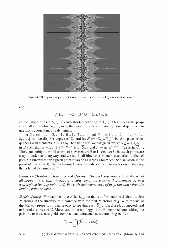
Figure 4. The dynamical plane of the map f : z �→ π sinh z. Several dynamic rays are shown.

and

f : Un,L → C \ (R− ∪ [−kπ i, kπ i]),so the image of each Un,× is a one-sheeted covering of Un,×. This is a useful prop-erty, called the Markov property, that aids in reducing many dynamical questions toquestions about symbolic dynamics.

Let ZR := {. . . , −2R, −1R, 0R, 1R, 2R, . . .} and ZL := {. . . , −2L , −1L , 0L , 1L,

2L , . . .} be two disjoint copies of Z, and let S := (ZR ∪ ZL)N be the space of se-quences with elements in ZR ∪ ZL . To each z in C we assign an itinerary s = s1s2s3 . . .

in S such that sk = nR if f ◦(k−1)(z) is in U n,R and sk = nL if f ◦(k−1)(z) is in U n,L .There are ambiguities if the orbit of z ever enters R or [−kπ i, kπ i], but such points areeasy to understand anyway, and we admit all itineraries in such cases (the number ofpossible itineraries for a given point z can be as large as four; see the discussion in theproof of Theorem 3). The following lemma furnishes a mechanism for understandingthe detailed dynamics of f :

Lemma 4 (Symbolic Dynamics and Curves). For each sequence s in S the set ofall points z in C with itinerary s is either empty or a curve that connects ∞ to awell-defined landing point in C. For each such curve each of its points other than thelanding point escapes.

Sketch of proof. For each positive N let Us,N be the set of points z such that the firstN entries in the itinerary of z coincide with the first N entries of s. With the aid ofthe Markov property it is quite easy to see that each U s,N is a closed, connected, andunbounded subset of C. Moreover, in the topology of the Riemann sphere, adding thepoint ∞ to these sets yields compact and connected sets containing ∞. Let

Cs :=⋂N∈N

(U s,N ∪ {∞}).


This is obviously a nested intersection, so Cs is compact and connected and contains∞. If Cs = {∞}, then we have nothing to prove. Otherwise, we can show that f isexpanding enough so that for any two points z and w in Cs and any η > 0 there isan n such that || Re f ◦n(z)| − | Re f ◦n(w)|| > η. Lemma 3 implies then that at leastone of the points z and w escapes. (The expansion comes from the fact that U :=C \ {−iπ, 0, iπ} carries a unique normalized hyperbolic metric and that f −1(U) ⊂ U .With respect to this metric on U , every local branch of f −1 is contracting, which makesf locally expanding. This argument requires nothing but the fact that the universalcover of U is D, plus the Schwarz lemma on holomorphic self-maps of D.)

It follows that all points in Cs \ {∞} escape, with at most one exception; the es-timates in Lemma 3 imply that these points escape extremely fast. This means thatfor almost all z in Cs \ {∞} we have f ◦n(z) → ∞ very fast, hence |( f ◦n)′(z)| → ∞very fast. Thus the forward iterates of z are very strongly expanding. Conversely, ifzn := f ◦n(z), then the branch of f −n sending zn to z is strongly contracting. This im-plies that the boundaries of the Us,N , which are curves, converge locally uniformly toCs . This ensures that Cs is a curve.

This lemma is all we need to establish the two main results about the dynamics ofthe function f .

Proof of Theorem 3. Every point z in C has at least one associated itinerary. If it hasmore than one, then under iteration it must map into iR or into R + 2π iZ. In thelatter case, the next iteration lands in R, so the orbit reaches either the fixed point0 or one of the two dynamic rays R

+ or R−. If the orbit reaches iR, then from that

iteration on it spends its entire forward orbit in the interval [−kπ i, kπ i]; in particular,the orbit is bounded. Therefore, a point has four itineraries if and only if its orbiteventually terminates at 0. A point has two itineraries if it lands in the invariant interval[−kπ i, kπ i] (and has bounded orbit), or if it lands in R

+ ∪ R− and escapes. Every

other point has a single itinerary.Recall that the set of points with a given itinerary is a single dynamic ray consisting

of escaping points, together with the unique landing point of the ray (Lemma 4). Thisimplies that every point in C either lies on a unique dynamic ray or is the landing pointof one, two, or four dynamic rays. This proves statements 2 and 3 in the theorem.

For statement 1, we have constructed rays consisting of escaping points, and thepartition makes it clear that every ray has real parts tending to ±∞, while the imagi-nary parts are constrained to some interval of length π . It is clear that each escapingpoint either is on a unique ray or is the landing point of a ray; if a ray lands at an escap-ing point, then the landing point neither lies on any other ray nor is the landing pointof another ray. Therefore, each ray (possibly together with its endpoint) is containedin a path component of I . It is also true that each path component of I consists of asingle ray, possibly together with its endpoint. The proof of this fact requires someingredients from continuum theory (see [11, sec. 4]).

8. LEBESGUE MEASURE AND ESCAPING POINTS. From the point of view ofdynamical systems, an important question to ask is the following: What do most orbitsdo under iteration? From a topological vantage point, most points are on dynamicrays, rather than being endpoints of rays. On the other hand, since the union of therays has Hausdorff dimension 1, measure theory says that most points are endpointsof rays. However, as we will now see, even measure theory asserts that most points inC escape (for our maps z �→ kπ sinh z): this assertion is a combination of results ofMcMullen [18] and Bock [3]. As a result, almost all points are escaping endpoints of


rays. Along the way, we visit a result of Schubert [27], [28] that settles a conjecture ofMilnor [20, sec. 6] in the affirmative.

Theorem 4 (Lebesgue Measure of Escaping Points).

(1) For every map z �→ λez with λ �= 0 the set I of escaping points has two-dimensional Lebesgue measure zero but Hausdorff dimension 2 [18].

(2) However, for every map z �→ aez + be−z with ab �= 0 the set I has infinite two-dimensional Lebesgue measure [18]. For every strip S = {z ∈ C: α ≤ Im z ≤β} in C the two-dimensional Lebesgue measure of S \ I is finite [27], [28].

Sketch of proof. Choose ξ > 0, and set Hξ = {z ∈ C: Re z > ξ}. We show that forevery map E(z) = λ exp(z) and sufficiently large ξ the set Zξ := {z ∈ C: Re E◦n(z) >

ξ for all n} has measure zero. In fact, for each square Q in Hξ of side-length 2π withsides parallel to the coordinate axes the image E(Q) is a large annulus in C, andthe probability that a point z in Q has E(z) in Hξ is approximately 1/2. The chanceof surviving n consecutive iterations in Zξ is then 2−n (assuming independence ofprobabilities in the consecutive steps). Hence, the set of points z in Q whose entireorbits lie in Hξ has two-dimensional Lebesgue measure zero, and thus all of Zξ hastwo-dimensional Lebesgue measure zero. But since |E(z)| = |λ| exp(Re z), for everypoint z in I there must be an N such that E◦n(z) belongs to Zξ for all n with n ≥ N .Since I is a subset of

⋃n≥0 E◦−n(Zξ ), it has measure zero for exponential maps z �→

λez .The situation is different for E(z) = aez + be−z with ab �= 0: instead of throwing

away half of the points in every step, we can “recycle” (in a literal sense) most of them:this time |E◦n(z)| → ∞ implies that |Re E◦n(z)| → ∞. We use another parabola (orrather the complement thereof), namely,

P := {x + iy ∈ C: |y| < |x |2}.If z = x + iy with |x | sufficiently large is such that E(z) lies in P , then

|Re E(z)| ≥ |E(z)|1/2 ≈ e|x |/2 � |x |,so points that escape to ∞ within P do so quite rapidly. On the other hand, the imageof a square Q as in the first part (with real parts x greater than ξ or less than −ξ )is again an annulus, but the fraction of E(Q) within P is approximately 1 − e−|x |/2,so most of the points survive the first step. Among these, a fraction of 1 − e−(e−|x |/2)/2

survives the second step, and so on. The total fraction of points within Q that “getlost” from P under iteration is less than 1, from which we infer that I ∩ Q has positivetwo-dimensional Lebesgue measure [18]. To be more precise, we recursively define asequence (ξn) by ξ0 = ξ and ξn+1 = e|ξn |/2 for n = 1, 2, . . .. Then ξn > 2n−1ξ1 for alln, provided that ξ0 is sufficiently large. If

Qn := {z ∈ Q: E◦k(z) ∈ P for k = 0, 1, 2, . . . , n},then each z in Qn has |Re E◦n(z)| > ξn. This means that of all the points in Qn , afraction of at least 1 − e−ξn/2 = 1 − 1/ξn+1 survives one more iteration within P . Thus,denoting two-dimensional Lebesgue measure by μ, we get

μ(Qn)

μ(Q)> 1 − 1

ξ1− 1

ξ2− · · · 1

ξn> 1 − 2

ξ1= 1 − 2e−ξ0 .


Since⋂

n Qn is contained in I , it follows that

μ(I ∩ Q) > (1 − 2e−ξ0/2)μ(Q) :the set of escaping points has positive density in Q, hence I has positive (even infinite)two-dimensional Lebesgue measure.

In fact, we have shown much more: μ(Q \ I ) < 2e−ξ0/2μ(Q) [27], [28]. Therefore,for each horizontal strip S of height 2π the complement of I in S has finite Lebesguemeasure:

μ (z ∈ S \ I : |Re z| > ξ0) < 2π

∫ ∞

ξ0

2e−x/2 dx = 4πe−ξ0/2.

This proves the result.

Remark. Milnor [20, sec. 6] conjectured that for f (z) = sin z the set of points con-verging to the fixed point z = 0 has finite Lebesgue area in every strip S′ = {z ∈C: α ≤ Re z ≤ β}. Since sine and hyperbolic sine represent the same map in rotatedcoordinate systems, this follows from Schubert’s result.

We conclude with another special case in which the set I is so large that C \ I hasmeasure zero [24]:

Corollary 2 (Escaping Set of Full Measure). For maps

z �→ kπ sin z or z �→ kπ sinh z

with a nonzero integer k the set I ∩ E has full two-dimensional Lebesgue measure(i.e., the measure of C \ (I ∩ E) is zero).

Proof. We invoke a theorem of Bock [3]: for an arbitrary transcendental entire functionat least one of the following two statements holds: (i) almost every orbit is dense in C

or (ii) almost every orbit converges to ∞ or to one of the critical orbits (a critical orbitis the orbit of one of the two critical values ±kπ i). But since I has positive measure,case (i) cannot hold, so statement (ii) follows. For the map E : z �→ kπ sinh z (or,equivalently, z �→ kπ sin z) the two critical values map to the fixed point 0. However,since |E ′(0)| > 1 (i.e., the fixed point 0 is “repelling”), the only points whose orbitscan converge to 0 are those countably many points that land exactly on 0 after finitelymany iterations. Therefore, almost every orbit must escape.

ACKNOWLEDGMENTS. I would like to express my gratitude to Bogusia Karpinska for many interest-ing discussions and for allowing me to include her example in section 4. I would also like to thank CristianLeordeanu and Gunter Rottenfußer for their help with the illustrations in this article.

REFERENCES

1. K. Baranski, Trees and hairs for entire maps of finite order (2005, preprint); available at http://www.mimuw.edu.pl/~baranski/publ.html.

2. W. Bergweiler, Iteration of meromorphic functions, Bull. Amer. Math. Soc. (N.S.) 29 (1993) 151–188;updates available at http://analysis.math.uni-kiel.de/bergweiler/bergweiler.engl.html.

3. H. Bock, On the dynamics of entire functions on the Julia set, Results Math. 30 (1996) 16–20.4. R. Devaney, Sex : Dynamics, topology, and bifurcations of complex exponentials, Topology Appl. 110

(2001) 133–161.


5. R. Devaney, L. Goldberg, and J. Hubbard, A dynamical approximation to the exponential map by poly-nomials, MSRI Preprint (1986).

6. R. Devaney and M. Krych, Dynamics of exp(z), Ergodic Theory Dynam. Systems 4 (1984) 35–52.7. R. Devaney and F. Tangerman, Dynamics of entire functions near the essential singularity, Ergodic The-

ory Dynam. Systems 6 (1986) 489–503.8. A. Eremenko, On the iteration of entire functions, in Dynamical Systems and Ergodic Theory, Banach

Center Publications, Polish Scientific, Warsaw, 1989, 339–345.9. K. Falconer, Fractal Geometry. Mathematical Foundations and Applications, John Wiley, Chichester,

UK, 1990.10. P. Fatou, Sur l’iteration des fonctions transcendantes entieres, Acta Math. 47 (1926) 337–370.11. M. Forster, L. Rempe, and D. Schleicher, Classification of escaping exponential maps, Proc. Am. Math.

Soc., to appear; available at http://arxiv.org/abs/math.DS/0311427.12. J. G. Hocking and G. S. Young, Topology, Dover, Mineola, NY, 1988.13. B. Karpinska, Hausdorff dimension of the hairs without endpoints for λ exp(z), C. R. Acad. Sci. Paris

Ser. I Math. 328 (1999) 1039–1044.14. J. Kotus and M. Urbanski, Fractal measures and ergodic theory of transcendental meromorphic func-

tions, Transcendental Dynamics and Complex Analysis, volume in honour of Professor I. N. Baker, LMSLecture Note Series (to appear); available at http://www.math.unt.edu/~urbanski.

15. D. G. Larman, A compact set of disjoint line segments in E3 whose end set has positive measure, Math-ematika 18 (1971) 112–125.

16. B. Mandelbrot, The Fractal Geometry of Nature, W. H. Freeman, New York, 1983.17. Y. I. Manin, The notion of dimension in geometry and algebra, Bull. Am. Math. Soc. New Ser. 43 2 (2006)

139–161.18. C. McMullen, Area and Hausdorff dimension of Julia sets of entire functions, Trans. Amer. Math. Soc.

300 (1987) 329–342.19. , Complex Dynamics and Renormalization, Princeton University Press, Princeton, 1994.20. J. Milnor, Dynamics in One Complex Variable. Introductory Lectures, 2nd ed., Vieweg Verlag, Wies-

baden, 2000.21. G. Rottenfußer, J. Ruckert, L. Rempe, D. Schleicher, Dynamic rays of bounded-type entire functions,

Manuscript, submitted.22. G. Rottenfußer, On the Dynamical Fine Structure of Entire Transcendental Functions, Ph.D. thesis, In-

ternational University Bremen, 2005.23. G. Rottenfußer and D. Schleicher, Escaping points of the cosine family, Transcendental Dynamics and

Complex Analysis, volume in honour of Professor I. N. Baker, LMS Lecture Note Series (to appear);available at http://arxiv.org/abs/math.DS/0403012.

24. D. Schleicher, The dynamical fine structure of iterated cosine maps and a dimension paradox, Duke Math.J. 136 2 (2007) 343–356; available at http://arxiv.org/abs/math.DS/0406255.

25. D. Schleicher and M. Thon, Hausdorff dimension of escaping points of bounded type transcendentalfunctions, Manuscript, in preparation.

26. D. Schleicher and J. Zimmer, Escaping points of exponential maps, J. London Math. Soc. (2) 67 (2003)380–400.

27. H. Schubert, Uber das Maß der Fatoumenge trigonometrischer Funktionen, Diplomarbeit, UniversitatKiel, 2003.

28. , Area of Fatou sets of trigonometric functions, Proc. Am. Math. Soc., to appear.29. G. Stallard, Dimensions of Julia sets of transcendental meromorphic functions, Transcendental Dynamics

and Complex Analysis, volume in honour of Professor I. N. Baker, LMS Lecture Note Series (to appear).30. M. Urbanski, Measures and dimensions in conformal dynamics (2003, preprint); available at http:

//www.math.unt.edu/~urbanski.

DIERK SCHLEICHER studied physics and mathematics in Hamburg and Cornell, with semesters abroad inPrinceton and Paris. He held teaching and research positions in Munich and Stony Brook, before moving toBremen in 2001 to help build up International University Bremen (now renamed as Jacobs University Bremen):a small and exciting new university with strong students from 80 countries. He has spent research semestersin Berkeley, Paris, and Toronto. His research interests are on the interplay between geometry and dynamics,with a focus on holomorphic dynamics and symbolic dynamics. On campus, he enjoys spending time withhis student advisees and organizing events like the International Mathematics Olympiad 2009 in Bremen; offcampus, he likes kayaking, paragliding, and hiking in the mountains.Jacobs University Bremen (formerly International University Bremen), Research I, Postfach 750 561, D-28725Bremen, [email protected]


Documents

Hausdorff Dimension, Its Properties, and Its Surprises