Embed Size (px)
Citation preview

IMPERIAL COLLEGE LONDON
UNIVERSITY OF LONDON
ON-LINE MEASUREMENTS OF CONTENTSINSIDE PIPES USING GUIDED ULTRASONIC
WAVES
by
Jian Ma
A thesis submitted to the University of London for the degree of
Doctor of Philosophy
Department of Mechanical Engineering
Imperial College London
London SW7 2BX
October 2007

Abstract
There have been extensive demands from industries to determine information about
the contents inside pipelines and it would be a great benefit if on-line measurements
could be made. Guided ultrasonic wave measurements can potentially fulfill such
a purpose since they are non-intrusive and can be carried out from outside of the
pipe wall. This thesis investigates the principles and develops new guided wave
techniques for two specific applications.
The first application relates to the fluid characterisation inside pipes. A new guided
wave technique is developed to measure the acoustic properties (bulk sound velocity
and shear viscosity) of fluids inside pipes. It is based on the measurements of the
velocity dispersion and attenuation of guided longitudinal modes in the pipe. It
allows the fluid properties to be characterised without taking samples out of the
pipe and can be employed both when the pipe is completely filled or when the filling
is local. In the latter case, the technique is exploited as a pipe ’dipstick’ sensor
dipped into the fluid to be measured. The dipstick sensor has the advantages that
the velocity measurement requires a single pulse echo measurement without the need
for knowing the depth of immersion of the pipe into the fluid.
The second application is for sludge and blockages detection in long-range pipelines.
Existing techniques have the limitations that the sludge position needs to be known
a priori and the area to be inspected needs to be accessible. Two guided wave tech-
niques have been developed which allow the the sludge or blockages to be detected
remotely without the need to access the specific location where the pipe is blocked,
nor to open the pipe. The first technique measures the reflection of guided waves by
sludge or blockages which can be used to accurately locate the blocked region; the
second technique detects sludge by revealing the changes to the transmitted guided
waves propagating in the blocked region or after it. The two techniques complement
each other and their combination leads to a reliable sludge or blockage detection.
Various types of realistic sludge or blockages have been considered in the study and
the practical capabilities of the two techniques have been demonstrated.
2

Acknowledgments
I would like to sincerely thanks my supervisor Professor Mike Lowe and my co-
advisors Dr. Francesco Simonetti and Professor Peter Cawley for their invaluable
guidance and for offering me a chance to study in the well organised Non-destructive
Testing Lab.
I would also like to thank my project collaborators, Professor Richard Challis from
Nottingham University and Dr. Sam Worthington from British Nuclear Fuel Ltd
(BNFL) for the discussions and insightful suggestions.
Also I acknowledge the input of my current and former colleagues in the NDT group
at Imperial College, which significantly benefited the completion of this project. In
particular, I am very grateful to Dr. Jimmy Fong, Dr. Mark Evans, Dr. Frederic
Cegla, Mr. Prabhu Rajagopal who helped me so much when I was lost at the early
stage of my Ph.D.
Furthermore, I must acknowledge the Engineering and Physical Sciences Research
Council (EPSRC) and BNFL which funded this work.
I also appreciate Professor Zhemin Zhu at Nanjing University who introduced me
into the field of acoustics has enlightened me with so much knowledge.
Finally, I would like to express my personal thanks to my parents and also to Xinxin
for their continued encouragement and support throughout my study. Wish all my
little progress will make you smile.
3
Contents
1 Introduction 22
1.1 Motivation . . . . . . . . . . . . . . . . . . . . . . . . . . . . . . . . . 22
1.2 Aim of the Investigation . . . . . . . . . . . . . . . . . . . . . . . . . 25
1.3 Outline of Thesis . . . . . . . . . . . . . . . . . . . . . . . . . . . . . 26
2 Guided Wave Propagation in Pipes Filled with Fluid 28
2.1 Background . . . . . . . . . . . . . . . . . . . . . . . . . . . . . . . . 28
2.2 Wave Propagation in Infinite Media . . . . . . . . . . . . . . . . . . . 29
2.3 Guided Waves in Cylindrical Pipes . . . . . . . . . . . . . . . . . . . 32
2.3.1 Guided waves . . . . . . . . . . . . . . . . . . . . . . . . . . . 32
2.3.2 Mode shape . . . . . . . . . . . . . . . . . . . . . . . . . . . . 35
2.3.3 Dispersion . . . . . . . . . . . . . . . . . . . . . . . . . . . . . 36
2.4 Guided Wave Propagation in Pipes Filled with Inviscid Fluid . . . . . 37
2.4.1 Dispersion curves . . . . . . . . . . . . . . . . . . . . . . . . . 38
2.4.2 Mode jumping . . . . . . . . . . . . . . . . . . . . . . . . . . . 38
2.4.3 Energy flow distribution . . . . . . . . . . . . . . . . . . . . . 39
2.5 Guided Wave Propagation in Pipes Filled with Viscous Fluid . . . . . 41
4

CONTENTS
2.5.1 Low-viscosity fluid . . . . . . . . . . . . . . . . . . . . . . . . 41
2.5.2 Highly viscous fluid . . . . . . . . . . . . . . . . . . . . . . . . 42
2.5.3 Density of fluid . . . . . . . . . . . . . . . . . . . . . . . . . . 44
2.6 Summary . . . . . . . . . . . . . . . . . . . . . . . . . . . . . . . . . 44
3 Characterisation of Fluids inside Pipes Using Guided Longitudinal
Waves 58
3.1 Background . . . . . . . . . . . . . . . . . . . . . . . . . . . . . . . . 58
3.2 Basic Principles of Ultrasound Measurements . . . . . . . . . . . . . 59
3.3 Ultrasound Measurements of Contents inside Pipe . . . . . . . . . . . 61
3.4 Experimental Setup . . . . . . . . . . . . . . . . . . . . . . . . . . . . 63
3.5 Measurement Methods . . . . . . . . . . . . . . . . . . . . . . . . . . 65
3.5.1 Measurement of longitudinal bulk velocity . . . . . . . . . . . 65
3.5.2 Measurement of viscosity . . . . . . . . . . . . . . . . . . . . . 68
3.6 Results . . . . . . . . . . . . . . . . . . . . . . . . . . . . . . . . . . . 69
3.6.1 Distilled water . . . . . . . . . . . . . . . . . . . . . . . . . . 69
3.6.2 Glycerol . . . . . . . . . . . . . . . . . . . . . . . . . . . . . . 70
3.6.3 Highly viscous fluid . . . . . . . . . . . . . . . . . . . . . . . . 72
3.7 Summary . . . . . . . . . . . . . . . . . . . . . . . . . . . . . . . . . 73
4 Scattering of the Fundamental Torsional Mode by an Axisymmetric
Layer inside a Pipe 80
4.1 Background . . . . . . . . . . . . . . . . . . . . . . . . . . . . . . . . 80
4.2 Torsional Waves in the Bilayered Pipe . . . . . . . . . . . . . . . . . 81
5

CONTENTS
4.3 Scattering of the T(0,1) Mode at the Discontinuity . . . . . . . . . . 85
4.3.1 Reflected signal . . . . . . . . . . . . . . . . . . . . . . . . . . 85
4.3.2 Local and transmitted signals . . . . . . . . . . . . . . . . . . 87
4.4 Experiments . . . . . . . . . . . . . . . . . . . . . . . . . . . . . . . . 88
4.4.1 Reflected signal: experimental results . . . . . . . . . . . . . . 90
4.4.2 Local signal: experimental results . . . . . . . . . . . . . . . . 92
4.5 Conclusion . . . . . . . . . . . . . . . . . . . . . . . . . . . . . . . . . 93
5 Feasibility Study of Sludge and Blockage Detection inside Pipes
Using Guided Torsional Waves 105
5.1 Background . . . . . . . . . . . . . . . . . . . . . . . . . . . . . . . . 105
5.2 Model Study . . . . . . . . . . . . . . . . . . . . . . . . . . . . . . . . 106
5.2.1 Imperfect bonding state . . . . . . . . . . . . . . . . . . . . . 106
5.2.2 Varying thickness . . . . . . . . . . . . . . . . . . . . . . . . . 108
5.2.3 Varying thickness and varying bonding state . . . . . . . . . . 109
5.2.4 Non-symmetric circumferential profile . . . . . . . . . . . . . 110
5.3 Experiments . . . . . . . . . . . . . . . . . . . . . . . . . . . . . . . . 112
5.3.1 Model experiment . . . . . . . . . . . . . . . . . . . . . . . . . 113
5.3.2 Realistic experiment . . . . . . . . . . . . . . . . . . . . . . . 115
5.4 Discussion . . . . . . . . . . . . . . . . . . . . . . . . . . . . . . . . . 118
5.5 Conclusions . . . . . . . . . . . . . . . . . . . . . . . . . . . . . . . . 119
6 Feasibility of Sludge and Blockage Detection inside Pipes using
Guided Longitudinal Waves 141
6

CONTENTS
6.1 Background . . . . . . . . . . . . . . . . . . . . . . . . . . . . . . . . 141
6.2 Longitudinal Modes in the Bilayered Pipe . . . . . . . . . . . . . . . 142
6.3 Scattering of the Longitudinal Modes: Idealised Model . . . . . . . . 143
6.3.1 Reflection measurement . . . . . . . . . . . . . . . . . . . . . 144
6.3.2 Transmission measurement . . . . . . . . . . . . . . . . . . . . 145
6.4 Irregular Properties of the Layer . . . . . . . . . . . . . . . . . . . . . 146
6.4.1 Imperfect bonding state . . . . . . . . . . . . . . . . . . . . . 146
6.4.2 Varying thickness and bonding state . . . . . . . . . . . . . . 147
6.5 Presence of Fluid inside the Pipe . . . . . . . . . . . . . . . . . . . . 148
6.6 Experiments . . . . . . . . . . . . . . . . . . . . . . . . . . . . . . . . 150
6.7 Conclusions . . . . . . . . . . . . . . . . . . . . . . . . . . . . . . . . 152
7 Conclusions 168
7.1 Review of Thesis . . . . . . . . . . . . . . . . . . . . . . . . . . . . . 168
7.2 Summary of Findings . . . . . . . . . . . . . . . . . . . . . . . . . . . 169
7.2.1 Characterisation of fluid properties inside pipes . . . . . . . . 169
7.2.2 Sludge and blockages detection and characterisation inside pipes171
7.3 Future Work . . . . . . . . . . . . . . . . . . . . . . . . . . . . . . . . 174
A Finite Element Models of Guided Torsional Modes Propagating in
a Pipe Locally Coated inside with an Elastic Layer 176
A.1 2D Finite Element Models . . . . . . . . . . . . . . . . . . . . . . . . 176
A.1.1 Idealised model . . . . . . . . . . . . . . . . . . . . . . . . . . 176
A.1.2 Imperfect bonding . . . . . . . . . . . . . . . . . . . . . . . . 177
7

CONTENTS
A.1.3 Varying thickness . . . . . . . . . . . . . . . . . . . . . . . . . 177
A.1.4 Varying thickness and varying bonding . . . . . . . . . . . . . 178
A.2 3D Finite Element Model . . . . . . . . . . . . . . . . . . . . . . . . . 178
B Finite Element Models of Guided Longitudinal Modes Propagating
in a Pipe Locally Coated inside with an Elastic Layer 180
B.1 Idealised Model . . . . . . . . . . . . . . . . . . . . . . . . . . . . . . 180
B.2 Imperfect Bonding . . . . . . . . . . . . . . . . . . . . . . . . . . . . 181
B.3 Varying Thickness . . . . . . . . . . . . . . . . . . . . . . . . . . . . 182
B.4 Varying Thickness and Varying Bonding . . . . . . . . . . . . . . . . 182
B.5 Presence of Fluid inside the Pipe . . . . . . . . . . . . . . . . . . . . 182
References 184
List of Publications 193
8

List of Figures
2.1 Schematics showing the superposition of partial bulk waves to form
guided waves in a clean pipe (a) and (b) a pipe filled with contents. L,
SH and SV stand for bulk Longitudinal waves, Shear Vertical waves
and Shear Horizontal waves. . . . . . . . . . . . . . . . . . . . . . . . 46
2.2 Phase velocity dispersion curves of the longitudinal (black solid curves),
torsional (gray dashed line) and flexural modes (black dashed curves)
in an empty steel pipe (9 mm inner diameter and 0.5 mm thickness).
Material properties are given in Tab. 2.1. . . . . . . . . . . . . . . . . 46
2.3 (a) Displacement mode shapes at 0.8 MHz for the L(0,1) mode (b)
for the L(0,2) mode (c) for the T(0,1) mode (d) for the F(1,3) mode
in Fig. 2.2. (black solid line) axial displacement; (gray dashed line)
radial displacement; (black dotted line) circumferential displacement.
The radial positions 4.5 and 5.0 correspond to the inside and outside
surface of the pipe wall, respectively. . . . . . . . . . . . . . . . . . . 47
2.4 (a) Group velocity dispersion curves of the longitudinal (black solid
curves), torsional (gray dashed line) and flexural modes (black dashed
curves) in an empty steel pipe (9 mm inner diameter and 0.5 mm
thickness). Material properties are given in Tab. 2.1; (b) The signal
of the L(0,2) mode at point A in Fig. 2.4a after 1 meter of its propa-
gation; (c) The signal of the L(0,2) mode at point B in Fig. 2.4a after
1 meter of its propagation. . . . . . . . . . . . . . . . . . . . . . . . 48
9

LIST OF FIGURES
2.5 (a) Phase velocity and (b) group velocity dispersion curves of lon-
gitudinal modes in a steel pipe (9 mm inner diameter and 0.5 mm
thickness) filled with water (black solid curves). For comparison, the
longitudinal modes in the empty pipe are also given (gray dashed
curves). Material properties are given in Tab. 2.1. . . . . . . . . . . . 49
2.6 Phase velocity dispersion curves of longitudinal modes in a steel pipe
(9 mm inner diameter and 0.5 mm thickness) filled with water (gray
solid curves). Two family of asymptotic modes are also shown as
free pipe modes (black dashed curves) and modes in the fluid column
(black solid curves). . . . . . . . . . . . . . . . . . . . . . . . . . . . . 50
2.7 (a) Energy flow ratio (EFR) of the selected modes in the steel pipe
filled with water; (b) corresponding phase velocity dispersion curves of
the selected modes (gray solid curves) and two families of asymptotic
modes, being free pipe modes (black dashed curves) and modes in the
fluid column (black solid curves). . . . . . . . . . . . . . . . . . . . . 51
2.8 Energy velocity dispersion curves of longitudinal modes in a steel pipe
(9 mm inner diameter and 0.5 mm thickness) filled with a inviscid
fluid (gray dashed curves) and with a low-viscosity fluid (black solid
line) (viscosity η = 1Pas). Material properties are given in Tab. 2.1. 52
2.9 (a) Energy velocity dispersion curves (above the branching points)
of longitudinal modes in a steel pipe filled with a low viscosity fluid
(η = 1Pas) for different values of longitudinal bulk velocity of the
fluid Cl = 1450m/s (solid line); Cl = 1500m/s (dashed line);(b)
Attenuation of longitudinal modes (above the branching points) in a
steel pipe filled with a fluid (Cl = 1500m/s) with different value of
viscosity η = 1Pas(solid line); η = 1.2Pas(dashed line). . . . . . . . . 53
2.10 Displacement mode shapes of selected points on Fig. 2.9b. (a) Mode
shape of point A. (b) Mode shape of point B. (solid line) axial dis-
placement; (dashed line) radial displacement. . . . . . . . . . . . . . . 54
10

LIST OF FIGURES
2.11 (a) Energy velocity dispersion curves of longitudinal modes in a steel
pipe filled with highly viscous fluid (Cl = 1500m/s) with different
values of viscosity. (η = 25Pas(black solid line ); η = 20Pas(gray
dashed line)); (b) Attenuation of the L3 mode in Fig. 2.11a. (α =
25Pas(black solid line); α = 20Pas(gray dashed line)) . . . . . . . . . 55
2.12 Phase velocity dispersion curves of longitudinal modes in a steel pipe
filled with highly viscous fluid (Cl = 1500m/s, η = 25Pas) (gray solid
curves). Two family of asymptotic modes are also shown as free pipe
modes (black dashed curves) and modes in the fluid column (black
solid curves). . . . . . . . . . . . . . . . . . . . . . . . . . . . . . . . 56
2.13 Energy velocity dispersion curves (above the branching points) of
longitudinal modes in a steel pipe filled with a low viscosity fluid
(Cl = 1450m/s, η = 1Pas) for different values of density of the fluid
ρ = 1g/cm3 (black solid line); ρ = 0.7g/cm3 (gray dashed line). . . . 57
3.1 Schematic of the experimental setup. . . . . . . . . . . . . . . . . . . 75
3.2 The sequence of propagation of longitudinal modes in a pipe partially
immersed into a fluid. . . . . . . . . . . . . . . . . . . . . . . . . . . 75
3.3 Amplitude spectrum of end reflection signal from a steel pipe im-
mersed into water (black line) and the branching frequency best fit
calculated by DISPERSE (dashed gray line). . . . . . . . . . . . . . 76
3.4 Reassigned spectrogram analysis of end reflection signal from a steel
pipe immersed into water and best fit curves (white dashed curves)
calculated with DISPERSE. . . . . . . . . . . . . . . . . . . . . . . . 76
3.5 Amplitude spectrum of end reflection signal from a steel pipe im-
mersed into glycerol (black line) and the branching frequency best fit
calculated with DISPERSE (dashed gray line). . . . . . . . . . . . . . 77
3.6 Reassigned spectrogram analysis of end reflection signal from a steel
pipe immersed into glycerol and best fit curves (white dashed curves)
calculated with DISPERSE. . . . . . . . . . . . . . . . . . . . . . . . 77
11

LIST OF FIGURES
3.7 Measured (black square) and theoretically predicted (black line) at-
tenuation of longitudinal modes in a steel pipe immersed into glycerol
(predictions by DISPERSE). . . . . . . . . . . . . . . . . . . . . . . . 78
3.8 Amplitude spectrum of end reflection signal from a steel pipe im-
mersed into a commercial Cannon VP8400 viscosity standard (black
line) and the branching frequency best fit calculated by DISPERSE
assuming that the fluid has no viscosity (dashed black line). The
branching frequency best fit calculated with DISPERSE using the
measured viscosity η = 18.8Pas for the fluid (dashed gray line). . . . 78
3.9 Reassigned spectrogram analysis of end reflection signal from a steel
pipe immersed into a commercial Cannon VP8400 viscosity stan-
dard and the analytical curves (white dashed curves) calculated with
DISPERSE using the measured values of longitudinal bulk velocity
(Cl = 1525m/s) and viscosity (η = 18.8Pas)for the fluid. . . . . . . . 79
3.10 Measured (black square) and theoretically predicted (by DISPERSE
using the initially measured longitudinal bulk velocity Cl = 1530m/s
for the fluid) attenuation of longitudinal modes in a steel pipe im-
mersed into a commercial Cannon VP8400 viscosity standard. (η =
18Pas (dashed gray line); η = 18.8Pas (black line); η = 20Pa.s
(dashed black line)) . . . . . . . . . . . . . . . . . . . . . . . . . . . . 79
4.1 Schematic of the model investigated in this chapter. . . . . . . . . . . 95
4.2 (a) Group velocity dispersion curves of torsional modes in an alu-
minum pipe (Inner diameter 16mm and thickness 1.4mm) coated with
a 6-mm thickness epoxy layer inside. Material properties are given
in Table 4.1. For comparison, the torsional mode in a pipe without
coating is also shown, by the dashed line. (b) Energy flow ratio. . . . 96
4.3 Energy flow density mode shapes for bilayered pipe, at points labelled
in Fig. 4.2b. (a) Mode shape of point A on the T2 mode. (b) Mode
shape of point B on the T1 mode. (c) Mode shape of point C on the
T2 mode. . . . . . . . . . . . . . . . . . . . . . . . . . . . . . . . . . . 97
12

LIST OF FIGURES
4.4 (a) Time trace, simulated by FE modelling, of the scattering of T(0,1)
in an aluminium pipe partially coated with a 6-mm thickness epoxy
layer inside, showing the incident and reflected signals received at the
Reflection measurement point in Fig. 4.1; (b) Corresponding reflec-
tion coefficient amplitude spectrum. F2, F3 are cut-off frequencies of
the bilayered pipe. . . . . . . . . . . . . . . . . . . . . . . . . . . . . 98
4.5 (a) Time trace, simulated by FE modelling, of the transmitted sig-
nal propagating past the bilayered part of a pipe; (b) Reassigned
spectrogram analysis of the transmitted signal and the correspond-
ing analytical calculation (white dashed curves) by DISPERSE; (c)
Reassigned spectrogram analysis of the incident signal of the T(0,1)
mode in the clean pipe (FE signal). . . . . . . . . . . . . . . . . . . . 99
4.6 Schematic of the experimental setup. . . . . . . . . . . . . . . . . . . 100
4.7 (a) A typical time-domain signal of the reflection measurement, show-
ing the incident signal and the reflected signal by the layer; (b)Reflection
coefficient amplitude of the T(0,1) mode from the aluminium pipe
coated inside with a 6-mm thickness epoxy layer, obtained by exper-
imental measurement (line with black squares) and FE calculation
(black solid line). . . . . . . . . . . . . . . . . . . . . . . . . . . . . . 101
4.8 Reflection coefficient amplitude of the T(0,1) mode from the alu-
minum pipe completely filled with epoxy over part of its length, ob-
tained by experimental measurement (line with black squares), FE
calculation assuming an elastic coating (black solid line) and FE cal-
culation assuming a viscoelastic coating (gray dashed line). . . . . . . 102
4.9 (a) Time-domain signal measured in the bilayered part of the alu-
minium pipe locally coated inside with a 6-mm thickness epoxy layer;
(b) Reassigned spectrogram analysis of the measured local signal
shown in Fig. 4.9a and analytical calculation (white dashed lines)
by DISPERSE. . . . . . . . . . . . . . . . . . . . . . . . . . . . . . . 103
13

LIST OF FIGURES
4.10 (a) Time-domain signal measured in the filled part of the aluminium
pipe locally filled with epoxy; (b) Reassigned spectrogram analysis
of the measured local signal and best fit curves (white dashed lines)
calculated by DISPERSE for the aluminum pipe locally filled with
epoxy. . . . . . . . . . . . . . . . . . . . . . . . . . . . . . . . . . . . 104
5.1 Schematic of the model in which the pipe is locally coated with 6-mm
thickness epoxy with an imperfect bonding state. . . . . . . . . . . . 121
5.2 Dispersion curves of the first two torsional modes in the pipe coated
with 6-mm thickness epoxy layer for different bonding states. Case 1:
perfect bonding, shear stiffnessKT ∈ ∞; Case 2: KT = 0.71GPa/mm;
Case 3: KT = 0.355GPa/mm; Case 4: KT = 0.071GPa/mm. . . . . 121
5.3 (a) Reflection coefficient spectrum obtained from FE simulations for
the T(0,1) mode when incident at the region where the pipe is lo-
cally coated with 6-mm thickness epoxy layer, for different bond-
ing states. Case 1: perfect bonding, shear stiffness KT ∈ ∞; Case
2: KT = 0.71GPa/mm; Case 3: KT = 0.355GPa/mm; Case 4:
KT = 0.071GPa/mm; (b)Reassigned Spectrogram analysis of the
transmitted signal in the pipe locally coated with 6-mm thickness
epoxy layer with imperfect bonding state (case 2) and the correspond-
ing numerical calculation with DISPERSE (white dashed curves). . . 122
5.4 (a) Schematic of the model in which the pipe is locally coated by
an epoxy layer that has varying thickness. The tapered region of
the bilayered pipe can be thought of as a succession of local uniform
bilayered pipes; (b) Schematic of the model in which the pipe is lo-
cally coated by an epoxy layer that has varying thickness and varying
bonding state. . . . . . . . . . . . . . . . . . . . . . . . . . . . . . . . 123
5.5 (a) Time trace of the incident and the reflected signals monitored at
the reflection measurement point in Fig. 5.4a; (b) Reassigned Spectro-
gram analysis of the transmitted signal monitored at the transmission
measurement point in Fig. 5.4a. . . . . . . . . . . . . . . . . . . . . . 124
14

LIST OF FIGURES
5.6 Cutoff frequency of the second torsional modes in the pipe coated
with epoxy layer as a function of the thickness of the layer. . . . . . . 125
5.7 (a) Time trace of the incident and the reflection signals monitored at
the reflection measurement point in Fig. 5.4b; (b) Reassigned Spectro-
gram analysis of the transmitted signal monitored at the transmission
measurement point in Fig. 5.4b. . . . . . . . . . . . . . . . . . . . . . 126
5.8 (a) Dispersion curves of the torsional modes in a 3 inch aluminium
pipe coated with 10-mm thickness epoxy layer (black curves) and
the T(0,1) mode in the clean 3 inch pipe (gray dashed line); (b)
Reflection coefficient amplitude spectrum of the T(0,1) mode in the
3 inch aluminium pipe coated with 10-mm thickness sludge layer for
different circumferential extents. Case 1: 100% (solid line: 3D model,
dotted line: 2D model), Case 2: 75%, Case 3: 50%, Case 4: 25%. . . 127
5.9 (a) Schematic of the model in which the pipe is partially coated with
an epoxy layer that has 50% circumferential extent; (b) Schematic of
the model in which the pipe is coated with an epoxy layer that has
10-mm thickness and 5-mm thickness, each for 50% circumferential
extent. . . . . . . . . . . . . . . . . . . . . . . . . . . . . . . . . . . 128
5.10 (a) Reassigned Spectrogram analysis of the transmitted T(0,1) mode
in the 3 inch pipe partially coated with 10-mm thickness epoxy layer
that has 100% circumferential extent and the corresponding numerical
calculation with DISPERSE (white dashed curves); (b) 75% circum-
ferential extent;(c) 50% circumferential extent ; (d) 25% circumfer-
ential extent. . . . . . . . . . . . . . . . . . . . . . . . . . . . . . . . 129
15

LIST OF FIGURES
5.11 (a) Reflection coefficient amplitude spectrum of the T(0,1) mode cal-
culated from the signals monitored at the reflection measurement
point in Fig. 5.9. For comparison, reflection coefficient spectra are
also calculated from two cases in which the layer respectively has 10-
mm thickness for 100% circumferential extent (black solid curves) and
5-mm thickness for 100% circumferential extent (gray solid curves);
(b) Reassigned Spectrogram analysis of the signals monitored at the
transmission measurement point in Fig. 5.9. . . . . . . . . . . . . . . 130
5.12 Reflection coefficient amplitude of the T(0,1) mode reflected by a
6-mm thickness epoxy layer inside an aluminium pipe. Experimen-
tal results with perfect bonding case (line with black squares) and
imperfect bonding (line with circles) case. The reflection coefficient
spectra amplitude from FE models for both cases are also provided
for comparison (solid lines). . . . . . . . . . . . . . . . . . . . . . . . 131
5.13 (a) Reassigned Spectrogram of the transmitted signal measured in
the blocked pipe region; (b) Reassigned Spectrogram of the incident
signal before the blocked pipe region. . . . . . . . . . . . . . . . . . . 132
5.14 Schematic of the measurements conducted on the pipe with randomly
shaped sludge layer made of simulant representing a real sludge material.133
5.15 (a) Time trace showing the incident signal and the reflected signals
measured at reflection measurement point in Fig. 5.14; (b) Reflec-
tion coefficient spectra magnitude of reflection 1 and reflection 2 in
Fig. 5.15a. . . . . . . . . . . . . . . . . . . . . . . . . . . . . . . . . . 134
5.16 Reassigned spectrogram analysis of the local signal measured at trans-
mission measurement point in Fig. 5.14 . . . . . . . . . . . . . . . . . 135
16

LIST OF FIGURES
5.17 (a) Speculated axial profile of the sludge made up by the simulant of
real sludge in the 3 inch steel pipe; (b) End view photography the
blocked pipe with the sludge layer; (c) The setup of the reflection
measurement using commercial WaveMaker Pipe Screening system
to detect the sludge inside the 3.5 inch pipe; (d) The setup of the
transmission measurement. . . . . . . . . . . . . . . . . . . . . . . . . 136
5.18 (a) Schematic of the reflection measurements conducted on a 3 inch
pipe with a sludge layer made of simulant of real sludge material, us-
ing commercially available guided wave transducer rings; (b) Schematic
of the transmission measurements using a pair of transducer rings. . 137
5.19 (a) Testing result of the reflection measurement conducted on the 3
inch pipe with sludge using a single commercially available guided
wave transducer ring as shown in Fig. 5.18; (b) Reflection coefficient
of the measured reflected T(0,1) mode from the sludge at two different
times (line with stars): first measurement; (line with black squares):
second measurement. . . . . . . . . . . . . . . . . . . . . . . . . . . . 138
5.20 (a) Reassigned spectrogram analysis of the transmitted signal con-
ducted on the clean part of the 3 inch pipe with sludge layer using
two guided wave transducer rings; (b) as in (a) but the measurement
were conducted on the blocked part of the pipe. . . . . . . . . . . . . 139
5.21 Standard deviations of arrival time (SDT) of the signals in Figs. 5.20a
and b (black curves), when different values of threshold are used to
extract the dispersion curves from the reassigned spectrogram. The
corresponding ratio (SDTR) is also given (gray dashed curve). . . . . 140
17

LIST OF FIGURES
6.1 (a) Group velocity dispersion curves of the longitudinal modes in an
aluminum pipe (Inner diameter 16mm and thickness 1.4mm) coated
with a 5-mm thickness epoxy layer inside (black solid curves). For
comparison, the longitudinal modes in a pipe without coating are also
shown (dashed curves). Material properties are given in Table 6.1.
(b) Dispersion curves of the L1 mode for different bulk velocities.
Bulk longitudinal velocity Cl = 2610m/s and bulk shear velocity
Cs = 1100m/s (black solid curve); Cl = 2610m/s and Cs = 1000m/s
(gray dashed curve); Cl = 4000m/s and Cs = 1100m/s (black dotted
curve). . . . . . . . . . . . . . . . . . . . . . . . . . . . . . . . . . . . 153
6.2 (a) Reflection coefficient spectrum obtained from FE simulations,
when the L(0,1) mode is incident at the region where the pipe is
locally coated with 5-mm thickness epoxy layer, for different bonding
states. Case 1: Perfect bonding ; Case 2: KN = 5GPa/mm, KT =
1.4GPa/mm; Case 3: KN = 2.5GPa/mm, KT = 0.7GPa/mm. (b)
As a, but for the case when the L(0,2) mode is incident. . . . . . . . 154
6.3 (a) Energy flow ratio (FER) of the longitudinal modes in Fig. 6.1a. . 155
6.4 (a) Reassigned spectrogram analysis of the FE simulated transmitted
signals monitored at the transmission measurement point in Fig. 4.1,
assuming the layer is not present. (b) Reassigned spectrogram analy-
sis of the FE simulated transmitted signals monitored at the transmis-
sion measurement point in Fig. 4.1. The comparisons with numerical
calculations (white dashed curves) is provided by DISPERSE. . . . . 156
6.5 Reassigned spectrogram analysis of the FE simulated transmitted
signals of longitudinal modes monitored at the transmission mea-
surement point in Fig. 5.1 (KN = 5GPa/mm, KT = 1.4GPa/mm)
and the corresponding numerical calculation with DISPERSE (white
dashed curves). . . . . . . . . . . . . . . . . . . . . . . . . . . . . . . 157
18

LIST OF FIGURES
6.6 (a) Group velocity dispersion curves of the longitudinal modes (black
solid curves) in an aluminum pipe coated with a 5-mm thickness epoxy
layer inside. A slip bonding is assumed at the bilayer interface. The
modes in the corresponding free pipe are also given (gray dashed
curves); (b) Displacement mode shape at point A (solid line) axial
displacement; (dashed line) radial displacement. . . . . . . . . . . . . 158
6.7 (a) Time-trace signals of the incident and the reflected signals mon-
itored at the reflection measurement point in Fig. 5.1, when the slip
bonding is assumed. The L(0,1) mode is selected as the incident
mode; (b) Reassigned Spectrogram analysis of the transmitted signal
monitored at the transmission measurement point in Fig. 5.1. . . . . 159
6.8 (a) Time-trace signals of the incident and the reflected signals mon-
itored at the reflection measurement point in Fig. 5.4a, when the
L(0,1) mode is incident; (b) Time trace of the incident and the
reflected signals monitored at the reflection measurement point in
Fig. 5.4b, when the L(0,1) mode is incident. . . . . . . . . . . . . . . 160
6.9 (a) Reassigned Spectrogram analysis of the transmitted signal moni-
tored at the transmission measurement point in Fig. 5.4a, using the
longitudinal modes for incidence. The numerical calculation of the
dispersion curve of the L(0,1) mode in the clean pipe is also pro-
vided by DISPERSE (white dashed curve);(b) Reassigned Spectro-
gram analysis of the transmitted signal monitored at the transmis-
sion measurement point in Fig. 5.4b, using the longitudinal modes for
incidence. . . . . . . . . . . . . . . . . . . . . . . . . . . . . . . . . . 161
6.10 Schematic of the model in which an aluminum pipe (Inner diameter
16mm and thickness 1.4mm) is filled with water and also is locally
coated by a 5-mm thickness epoxy layer. . . . . . . . . . . . . . . . . 162
6.11 Dispersion curves of the longitudinal modes in the water-filled pipe
(gray dashed curves) and the longitudinal modes in the water-layer
pipe (black solid curves). . . . . . . . . . . . . . . . . . . . . . . . . . 162
19

LIST OF FIGURES
6.12 (a) Time-trace signals of the incident and the reflected signals moni-
tored at the reflection measurement point in Fig. 6.10, when the Lw1
mode at its plateau region is used for incidence; (b) For the case when
the Lw4 mode at its plateau region is used for incidence. . . . . . . . . 163
6.13 (a) Reassigned Spectrogram analysis of the transmitted signal moni-
tored at the transmission measurement point in Fig. 6.10, when the
length of the water-filled region is 3 times that of the water-layer
region. The numerical calculation is also provided by DISPERSE
(white dashed curve);(b) as (a), for the case, when the length of the
water-filled region is 10 times that of the water-layer region. . . . . . 164
6.14 Schematic of the experiment measurements conducted on a pipe lo-
cally containing an epoxy tube that has varying thickness and imper-
fect bonding state. . . . . . . . . . . . . . . . . . . . . . . . . . . . . 165
6.15 (a) Reflection coefficient spectrum amplitude measured from the sam-
ple shown in Fig. 6.14, when the L(0,1) mode is incident; (b) Time-
trace signals of the reflection measurement conducted on the sample
shown in Fig. 6.14, when the L(0,2) mode is incident. . . . . . . . . . 166
6.16 (a) Reassigned Spectrogram analysis of the local signal measured from
the sample shown in Fig. 6.14; (b) Reassigned Spectrogram analysis
of the incident signals measured from the sample shown in Fig. 6.14
at the receiver point of the reflected signal. The numerical calculation
is provided by DISPERSE (white dashed curve). . . . . . . . . . . . . 167
20

List of Tables
2.1 Material properties of the steel pipe and the filling fluid used for
DISPERSE calculations. η and ρ are the viscosity and density of the
fluid respectively and ω is the circular frequency . . . . . . . . . . . . 35
3.1 Comparison of measured longitudinal bulk velocity and viscosity with
literature data and other independent measurements. Cl(AS) and
Cl(RS) are the longitudinal bulk velocity measured by amplitude spec-
trum and reassigned spectrogram respectively. . . . . . . . . . . . . . 71
4.1 Material properties of the aluminium pipe and epoxy layer used for
DISPERSE calculation and FE modelling. . . . . . . . . . . . . . . . 83
4.2 Material properties of the aluminium pipe and epoxy layer used for
FE calculations to compare with the remote measurement results.
The bulk shear velocity of epoxy was determined by an independent
measurement. . . . . . . . . . . . . . . . . . . . . . . . . . . . . . . . 89
6.1 Material properties used for DISPERSE calculations and FE simula-
tions. . . . . . . . . . . . . . . . . . . . . . . . . . . . . . . . . . . . . 143
21

Chapter 1
Introduction
1.1 Motivation
There are many circumstances in the process, power and oil industries, where it is
necessary to determine information about the material inside a pipeline and it would
be a great benefit if a non-intrusive measurement technique could be used to make
on-line measurements. There are two practical problems which particulary motivate
this thesis.
The first motivation comes from a need by many industries which is to determine the
material properties of fluids inside pipelines so as to help the monitoring and control
of processes. For example, much effort in the pharmaceutical industry has been
applied to the use of supercritical CO2 for the formation of polymers and advanced
copolymers [1, 2, 3], which has the advantage of avoiding the use of potentially
toxic solvents whilst at the same time minimising toxic residues from formation
processes. Supercritical water can be used to rapidly oxidise highly toxic materials
in a contained vessel or pipe without recourse to incineration with the risk of toxic
emissions. It is recognised that these new processes require monitoring and control.
In particular it is necessary to track fluid phase behavior under conditions of high
temperature and pressures, where the supercritical point may move in a complex
way in response to chemical association and reaction.
Many of the properties of the fluid can be surely found by opening the pipe, using
22

1. Introduction
devices which travel within the pipe, or tapping off samples. Once samples have
been taken, many techniques can be used to make the measurements. Ultrasonic
spectrometers using bulk ultrasonic waves have been commonly applied, for example,
to monitor the physical state of colloids and emulsions [4], and to track changes such
as flocculation [5] and crystallisation [6]. Ultrasound is capable of examining opaque
samples where standard optical techniques fail. But the extraction of samples from
the line introduces a delay to the measurements and so limits the feedback response
to process changes; furthermore, the measurements are not made under the line
conditions of pressure, temperature and flow which may change some properties of
the fluid when it is extracted from the line.
There are a number of on-line ultrasound measurement techniques available, which
will be reviewed in Sec. 3.3. However, these techniques are either intrusive to the
pipeline or are limited in the range range of material they can measure such as
highly attenuative fluid.
The second motivation of the thesis is to detect and even characterise sludge or
blockages inside pipelines. The accumulation of sludge inside pipelines is a problem
which commonly occurs in the chemical, process, oil and food industries. Ultimately
blockages can result from the accumulation of sludge. The sludge and blockages
can be formed by different materials depending on the types of the plants and the
processing conditions. For example, in the pipelines of petroleum plants, sludge is
often caused by precipitation of paraffins and asphaltenes in crude oil transportation
and processing [7]. Fuel corrosion products are found by some chemical companies
to be the main cause of the sludge at their plant [8].
The presence of sludge or blockages in pipelines has an impact on several of the
factors that affect the plant operation. The efficiency of the plant may be reduced
in terms of product flow rate, owing to the reduction in pipe diameter. The insulative
effect of the sludge or blockages may reduce the rate of heat transfer from the heat
exchanger to the product during heating, or vice versa during cooling. The quality
of the product may also be compromised as a result of changes in the processing
conditions. In addition, the product may become contaminated by pieces of the
sludge that detach from the pipe. In the extreme, the plant may become unsafe to
use.
23

1. Introduction
Once the sludge or blockage has occurred, the operating companies have to attend to
the pipeline as quickly as possible in order to restore appropriate flow conditions and
prevent a threat to the environment. There are a few remedial techniques available
in industry, such as external heating, coiled tubing intervention, pigging methods
and using dense chemical solvents [7]. However, the cleaning and replacement of
the blocked pipe often involves production down time, cleaning agents and possibly
some parts of the plant being stripped, all of which result in significant loss of plant
efficiency and increase the costs. Most important are the safety issues, such as the
possible catastrophic failure of a gas pipeline, which is a threat to personal health.
An effective sludge and blockage detection system is very important since it can
reduce production down time and costs. An accurate detection of sludge or blockages
may also avoid unnecessary cleaning which may be scheduled as a regular pipeline
maintenance to prevent the accumulation of sludge [9]. Also, without knowledge of
the location of the sludge, whole pipelines may have to be cleaned or even replaced.
Likewise, an early detection of a sludge problem in the pipeline avoids producing
unqualified products that have been contaminated by the sludge. Therefore a system
that can detect, locate and even monitor the accumulation of sludge build up is
desired.
Current techniques to detect sludge inside pipes are limited or intrusive. For exam-
ple, pipeline diameter expansion induced by internal pressurization of the pipe can
be measured point by point along the pipeline and correlated to the contents in the
pipe [10], but this method has the limitation that the location of the blocked region
needs to be known a priori and the area to be inspected needs to be accessible.
Alternatively, a technique termed acoustic pressure can be used. This technique
injects an acoustic pressure wave into the gas contained in a duct or a pipe and
measures the acoustic response of the duct. The presence of a blockage induces an
eigenfrequency shift in the response which can be used to reconstruct an image of
the blockage area [11, 12]. However, the method requires access to the inside of the
pipeline which is not possible in many practical situations.
24

1. Introduction
1.2 Aim of the Investigation
These two problems require techniques that can non-intrusively detect and measure
materials within pipelines. This thesis investigates the feasibility of using guided
ultrasonic waves which travel in the wall of the pipe for such a purpose. Guided
waves can be excited from the outside of the pipe wall at one location and propagate
along the length of the pipe for long distances. They are partially reflected when
they encounter features in the pipe (such as welds, corrosion, cracks, etc...) that
locally cause a discontinuity of the pipe wall. Technologies employing ultrasonic
guided waves have been well developed for the long-range inspection of pipeline
[13-18].
It would be very useful if guided waves could also be used to measure materials
inside pipes. Two guided wave measurement ideas can be pursued. First, the pres-
ence of contents will change the propagation characteristics of the guided waves in
the pipe, depending on the material properties of the contents. Thus, by quanti-
tatively measuring these propagation changes, some properties of the contents can
be obtained. This can be particulary useful for on-line fluid characterisation inside
pipelines, since the measurements are performed at the outer surface of the pipe and
are completely non-intrusive. Moreover, the guided wave measurements measure the
signal propagating in the pipe wall, unlike the bulk ultrasonic wave measurements,
which measure the signals traveling across the material under investigation directly.
Therefore, the guided wave measurements suffer much lower attenuation due to the
material damping of the content than the bulk ultrasonic wave measurements.
The second idea makes use of the fact that the localised accumulation of material
inside a pipe causes a change of the acoustic impedance of the pipe which scatters
the guided waves propagating in the pipe. The characteristics of both reflection and
transmission of the incident guided wave depend on the nature of the guided waves
and the properties of the pipe contents. Therefore, by analyzing both the reflection
and the transmission, the contents can be remotely detected, and even character-
ized in some situations. This provides a very attractive method for detecting and
characterising sludge and blockages in pipelines.
This thesis primarily aims at determining the feasibility of using guided waves to ad-
25

1. Introduction
dress the two mentioned industrial problems. However, the findings will be useful to
a large number of studies regarding ultrasonic wave propagation in filled waveguides.
For example, research [19, 20] has been carried out to investigate the possibility of
using guided ultrasonic waves to monitor the build-up of fouling films in heat ex-
changers and pipelines which is a widespread problem in ultra high-temperature
processing plants, particularly those used for milk and milk products [21]. The
fouling film has similar impacts on the operation of these plant as the sludge and
blockages considered in the thesis, although it largely consists of denatured whey
proteins and calcium deposits from milk and milk products. The work presented in
this thesis for sludge and blockages detection using guided waves should contribute
useful information to this topic.
1.3 Outline of Thesis
The thesis can generally be divided into two parts according to their applications.
Chapter 2 and 3 present the work for the purpose of fluid characterisation, while the
work in Chapters 4, 5 and 6 are mainly carried out for sludge and blockage detection
and characterization. Specifically, subsequent to the introductory remarks in this
chapter, the thesis is structured in the following way.
Chapter 2 reviews some basic concepts about bulk ultrasonic wave propagation
in unbounded media and guided ultrasonic wave propagation in cylindrical pipes.
In particular, the models of guided longitudinal waves propagating in pipes filled
with fluids are revisited to extract the physical principles which can be exploited to
develop a guided wave technique for fluid characterisation inside pipes.
Based on the principles identified in Chapter 2, a new guided wave technique to
measure the longitudinal bulk velocity and shear viscosity of fluids inside a pipe
is presented in Chapter 3. It is demonstrated that this guided wave technique is
capable of non-intrusively measuring both low-viscosity fluid and highly viscous fluid
inside the pipe. Some basic principles of ultrasound measurements and a review of
existing ultrasound methods for material characterisation inside pipes are also given.
Chapter 4 studies the scattering of the fundamental guided torsional mode by a local
26

1. Introduction
axisymmetrical elastic layer inside a pipe, which is a simplified model of sludge and
blockages inside pipes. The study reveals the physics of the problem and leads to two
measurement ideas which make use of both the reflection and transmission of the
torsional mode to characterize the geometry or acoustic properties of a layer inside
a pipe. The two ideas are investigated through both Finite Element simulations and
experimental measurements.
Chapter 5 proceeds the work in Chapter 4 by taking into account more realistic
sludge and blockage characteristics, such as their irregular profiles, bonding prob-
lems and the damping of the sludge material. The proposed reflection and transmis-
sion measurement ideas have also been implemented using commercial guided wave
equipment to demonstrate the practical capabilities. An overall assessment of using
guided torsional waves for practical sludge and blockage detection and characteriza-
tion is made.
Some results of using guided longitudinal waves for sludge and blockage detection
are presented in Chapter 6. The work is a generalization of the two measurement
ideas introduced in Chapters 4 and 5 when using guided torsional waves. The
measurement ideas are found to be also applicable when using the longitudinal
mode for sludge and blockages detection; however, the applicability is restricted
under the circumstance when fluid is present. The advantages and disadvantages of
the measurements using guided longitudinal waves compared to those using torsional
waves is concluded.
The main conclusions of the thesis are summarized in Chapter 7 where possible
future applications are also illustrated.
27

Chapter 2
Guided Wave Propagation in
Pipes Filled with Fluid
2.1 Background
This chapter introduces some basic concepts about bulk ultrasonic wave propagation
in unbounded media and guided ultrasonic wave propagation in waveguides, such as
cylindrical pipes.
In an unbounded elastic medium, bulk ultrasonic waves can propagate as homoge-
neous or inhomogeneous bulk longitudinal and shear waves. In a waveguide such as
a pipe, partial bulk waves reverberating between the boundaries of the waveguide
are superposed to form a guided wave propagating along the structure. There are
a large number of guided wave modes which can propagate in pipes with different
propagation characteristics. Features of guided wave modes in pipes such as their
velocity dependence on frequency, called dispersion, and the distribution of the field
variables over the cross section of the pipe, referred to as mode shape are introduced.
The propagation of guided wave modes in a pipe is affected by the media surround-
ing and inside the pipe. For the particular purpose of fluid characterisation inside
pipes, this chapter summarizes the main characteristics of the guided longitudinal
wave propagating in pipes filled with fluids. The main purpose is to extract some
physical principles which can be exploited to develop a guided wave technique for
28

2. Guided Wave Propagation in Pipes Filled with Fluid
fluid characterisation inside pipes that will be addressed in Chapter 3.
The Chapter starts with a brief introduction of bulk ultrasonic waves propagation
in an unbounded medium in Sec. 2.2. Then the propagation of guided waves in free
pipes is addressed in Sec. 2.3 followed by presentations of guided longitudinal waves
in pipes filled with different fluids, including inviscid fluid in Sec. 2.4 and viscous
fluid in Sec. 2.5.
2.2 Wave Propagation in Infinite Media
Wave propagation in unbounded, isotropic media is well documented in many text-
books (see, for example, Refs [22], [23], [24]) and is therefore only outlined briefly
in this section.
Starting in a Cartesian coordinate system the linearized equation of motion, the
particle displacement u in a material of density ρ is related to the stress tensor σ by
ρ∂2u
∂t2= ∇ · σ, (2.1)
∇ is the three dimensional differential operator. Hooke’s law can be used to relate
stresses to strains and displacements in an isotropic elastic medium as
σ = λI∇ · u + µ(∇u + u∇T), (2.2)
where λ and µ are Lame constants and I is the identity matrix. Combining equa-
tion 2.1 and equation 2.2 gives the Navier equation for displacement u
ρ∂2u
∂t2= (λ+ 2µ)∇(∇ · u) + µ∇2u. (2.3)
By means of the Helmholtz decomposition, the displacement field can be expressed
as a sum of the gradient of a compressional scalar potential φ, and the curl of an
equivoluminal vector H [25]
u = ∇φ+∇×H, (2.4)
29

2. Guided Wave Propagation in Pipes Filled with Fluid
with
∇ ·H = 0. (2.5)
By substituting equation 2.4 into equation 2.3, after some algebra, equation 2.3 can
be split into two equations for two unknown potentials
∂2φ
∂t2= c2l∇2φ, (2.6)
∂2H
∂t2= c2s∇2H, (2.7)
where
cl =
√λ+ 2µ
ρ, (2.8)
cs =
õ
ρ. (2.9)
cl and cs are the velocities of dilatational (longitudinal) and rotational (shear) waves
in the infinite isotropic medium. A general solution to equation 2.6 and equation 2.7
is
φ = φ0ei(kl·z−ωt), (2.10)
H = H0ei(ks·z−ωt), (2.11)
where φ0 and H0 are arbitrary constants and kl,s are wavenumber vectors which
satisfies the secular equations
kl,s · kl,s =ω2
c2l,s. (2.12)
where ω = 2πf is the angular frequency. In general the wavenumber k is a complex
vector
k = kren + ikimb, (2.13)
30

2. Guided Wave Propagation in Pipes Filled with Fluid
where kre and kim represent the real and imaginary part of the wavenumber in
the directions defined by unit vectors n and b respectively. The real part of the
wavenumber represents the phase propagation and the imaginary part on the other
hand represents a spatial attenuation. Equation 2.12 can thus be written as:
k2re + 2ikrekimn · b− k2
im =ω2
c2. (2.14)
This equation admits an infinite number of solution depending on the angle between
the vectors n and b. For an elastic medium, the right hand side of this equation
is pure real. It follows in this case that the real part of the wavenumber must be
orthogonal to the imaginary part
krekimn · b = 0. (2.15)
This results in two conditions for equation 2.14. Either kim = 0 which describes the
propagation of homogeneous plane waves, or kim 6= 0 but (n · b) = 0 which describes
an inhomogeneous wave whose attenuation vector kim is normal to the propagation
direction.
The above analysis can be extended to viscoelastic materials. The approach is
well described in the literature ( [26], [27], [28]) and hence only the results will
be mentioned here. As for elastic waves, the governing equations in the viscoelastic
case can be split up into shear and longitudinal waves with their respective velocities
cl =
√λ+ 2µ
ρ+ i
λ′ + 2µ′
ρ, (2.16)
cs =
õ
ρ+ i
µ′
ρ, (2.17)
where cl, cs are the complex longitudinal and shear bulk velocities respectively, ρ is
the density, λ and µ are the real Lame constants and λ′ and µ′ are the imaginary
Lame constants. i is defined as√−1. The Lame constants of viscoelastic material
are generally frequency dependent. This time the right hand term of equation 2.14
is complex and results in real and imaginary wavenumber vectors that are non zero
and in general n and b are neither parallel nor perpendicular.
31

2. Guided Wave Propagation in Pipes Filled with Fluid
2.3 Guided Waves in Cylindrical Pipes
2.3.1 Guided waves
Guided wave propagation in cylindrical waveguide structures has been treated by
many researchers ([29], [30],[31], [32]), and only a brief overview is given here. The
discussion here will be focused on the case of a cylindrical pipe which is the waveguide
studied in this thesis.
Since the equation 2.4 is separable in cylindrical coordinates, the solution may be
divided into the product of functions of each of the spatial dimensions in cylindrical
coordinates
φ,H = Γφ,H(r)Γφ,H(θ)Γφ,H(z)ei(k · r− ωt), (2.18)
where k is the wavenumber vector, and Γφ,H(r), Γφ,H(θ) and Γφ,H(z) describe the
field variation in each spatial coordinate. Assuming that the wave does not propa-
gate in the radial direction (r) and that the displacement field varies harmonically
in the axial (z) and circumferential (θ) directions, equation 2.18 can be written as
φ,H = Γφ,H(r)eiνθei(kz−ωt), (2.19)
where k is the component of the complex vector wavenumber in the z direction. ν
is referred to as the circumferential order which must be a whole number, since only
propagation in the direction of the axis of the cylinder is considered and the field
variables must be continuous in the angular direction.
Substituting these expressions of the potentials into equation 2.6 and equation 2.7,
Γ(r) can be expressed in terms of Bessel functions. For example, to demonstrate
the wave’s behavior for an axisymmetric guided wave mode, let ν = 0. Γφ,H(r) will
have the form [23]
Γφ(r) = A1J0(αr) + A2Y0(αr), (2.20)
ΓH(r) = B1J1(βr) +B2Y1(βr), (2.21)
32

2. Guided Wave Propagation in Pipes Filled with Fluid
where
α2 =ω2
cl2− k2, (2.22)
β2 =ω2
cs2− k2. (2.23)
Here Jm and Ym are Bessel functions of the first and second kind, respectively.
Recalling from equation 2.4 and Hooke’s law, the field variables such as displace-
ments and stresses can be expressed in terms of potential functions which are func-
tions of r satisfying the Bessel differential operator (for example, f(r),g1(r) and
g3(r) in reference [29]). Therefore, in general, the field variables, for example the
displacements, can be written as
Ur,θ,z = Ur,θ,z(r)eiνθei(kz−ωt). (2.24)
(2.25)
where Ur,θ,z(r) can be considered as radial distribution function of the displacement
in r, θ and z directions, respectively.
A waveguide can consist of a number of layers itself, e.g. the pipe may be filled with
liquid or solid contents (Fig. 2.1). The displacement and stress in each layer are ex-
pressed in terms of potential functions. The solutions for these potential functions
are substituted into these equations. This provides, in each layer of the waveguide,
six equations in terms of unknown partial wave amplitudes that correspond to the
coefficients of the Bessel functions used in the solution. The amplitudes, directions
and phases of the partial waves must be determined such that the boundary con-
ditions at the boundaries of the waveguide are satisfied, where Snell’s law must be
obeyed [25]. A guided wave in the waveguide therefore can be thought of as a super-
position of partial bulk waves which are reflected within the waveguide boundaries
(see Fig. 2.1).
In order to determine the guided waves in arbitrary multilayered system, a general
purpose software tool DISPERSE was developed by Lowe [33] and Pavlakovic [34,
33

2. Guided Wave Propagation in Pipes Filled with Fluid
35]. This is based on the ’global matrix method’ proposed by Knopoff [36], later
refined by Schmidt and Jensen [37]. The global matrix denoted [G] relates the
partial wave amplitudes to the physical constraints of the multilayered waveguide
and forms the equation
[G] {A} = 0, (2.26)
where {A} is a vector of the partial wave magnitudes. The above equation is satisfied
when the determinant of the global matrix vanishes, and solutions are sought in the
wavenumber-frequency space. If the material is absorbing, or the layer is immersed
so that it leaks waves into the surrounding medium, then the wavenumber becomes
complex whose imaginary part describes the attenuation of the guided wave. The
resulting roots are connected together to form dispersion curves of different guided
wave modes in the waveguide.
Three different families of modes are present in cylindrical waveguides: longitudinal,
torsional, and flexural modes. Each family of modes itself comprises an infinite
number of modes. The modal fields of longitudinal and torsional modes are constant
around the circumference, which means that the circumferential order ν is zero, while
the flexural modes are non-axisymmetric with ν ≥ 1.
As an example, Fig. 2.2 shows the phase velocity dispersion curves of guided wave
modes in a steel pipe surrounded by vacuum, predicted with DISPERSE. The ma-
terial properties for steel are given in Tab. 2.1. The phase velocity dispersion curves
show velocities of the wave cycles within a signal. The mode naming convention in
this thesis follows the one used by Silk and Bainton [32]. Longitudinal and torsional
modes are denoted as L(0,n) and T(0,n), respectively. In this notation, the first
number indicates the circumferential order, being zero for both longitudinal and
torsional modes, whereas the second number is a counter in order to distinguish
between the modes of the same family. Flexural modes are abbreviated according
to the notation F (ν, n) and only the first order flexural modes are plotted here.
34

2. Guided Wave Propagation in Pipes Filled with Fluid
Table 2.1: Material properties of the steel pipe and the filling fluid used for DISPERSE
calculations. η and ρ are the viscosity and density of the fluid respectively and ω is the
circular frequency
.
Longitudinal velocity(m/s) Shear velocity(m/s) Density(kg/m3)
Steel 5959 3260 7392
Viscous fluid 1500√
2ηωρ
1000
2.3.2 Mode shape
One effective method of examining the wave modes is to look at the mode shape
at each point on the dispersion curves. The mode shape displays how the displace-
ments, stress or energy vary through the thickness of the waveguide system. The
mode shapes are calculated to be of arbitrary absolute amplitude but show the
correct relative amplitude compared to another displacement or stress component.
The different mode families are best distinguished by considering the components
of their displacement mode shapes:
- Longitudinal (L) modes: Uz, Ur 6= 0 Uθ = 0
- Torsional (T) modes: Uθ 6= 0 Uz, Ur = 0
- Flexural (F) modes: Uz, Ur, Uθ 6= 0
All mode shape predictions are also calculated with DISPERSE. Fig. 2.3 shows as
an example, the displacement mode shapes of the L(0,1), L(0,2), T(0,1) and F(1,3)
modes respectively at 0.8 MHz in Fig. 2.2.
The displacement mode shape in Fig. 2.3a shows that at this frequency, the L(0,1)
mode is characterized predominantly by the radial displacement, while the L(0,2)
mode at the same frequency can be simply considered as an extensional mode as
shown in Fig. 2.3b: the axial displacement is dominant compared to the radial
displacement and nearly remains constant through the pipe wall. The T(0,1) mode
only has the displacement in the circumferential direction as shown in Fig. 2.3c. The
F(1,3) mode has displacement in all three directions (Fig. 2.3d).
35

2. Guided Wave Propagation in Pipes Filled with Fluid
2.3.3 Dispersion
The dispersion phenomenon is due to frequency-dependent velocity variations. In
1877 Lord Rayleigh [38] had already observed that the velocity of a group of waves
could be different from the velocity of the individual wave. He described the concepts
of phase (Cp) and group velocity (Cg). The phase velocity is the rate at which the
phase of the wave propagates in space, that is the velocity at which the phase of
any one frequency component of the wave will propagate. The group velocity is the
velocity at which a wave packet will travel at a given frequency and is the derivative
of the frequency wave-number dispersion relation. Phase and group velocities are
related to each other through the following equation (see [23] and [24] for more
details):
Cg = Cp + k∂Cp∂k
(2.27)
where k is the wavenumber.
Another commonly used concept is the energy velocity that is the velocity at which
the wave carries its potential and kinetic energy along the structure. Long range
testing usually makes use of finite tone bursts or wave packets and optimally exploits
waves at frequencies where there is little dispersion, thus the different frequency
components within the wave packet propagate at the same velocity and so the wave
packet retains its shape as it travels. Naturally it would be expected that the
energy to be transported at the speed of travel of the wave packet, and typically
in practice it is true to take this to be equal to the group velocity. However such
a relationship does not always hold. If an attenuating wave (caused by leakage
or material damping) is described, as is conventional, by a complex wave number,
then the group velocity calculation yields non-physical solutions, while the energy
velocity calculation is more stable and accurate [39].
Fig. 2.4a shows the group velocity dispersion curves for guided wave modes in
Fig. 2.2. Fig. 2.4a shows that, except the T(0,1) mode which is completely non-
dispersive, all the other guided wave modes have very different dispersion charac-
teristics at different frequencies. To illustrate this, Fig. 2.4b and c show (calculated
with DISPERSE) a 10 cycle toneburst signal of the L(0,2) mode monitored after 1
36

2. Guided Wave Propagation in Pipes Filled with Fluid
meter of its propagation with the central frequency of the signal respectively selected
at the non-dispersive region (point A, 650 kHz) and dispersive region (point B, 250
kHz) on the L(0,2) mode in Fig. 2.4a. The signal becomes dispersive in Fig. 2.4c,
which is exhibited by the increasing wave-packet duration and decreasing amplitude.
The effect of dispersion is undesirable for guided waves, since the energy in a dis-
persive wave-packet is not conserved as it propagates at different speeds depending
on the frequency. The amplitude of the wave-packet reduces as the signal propa-
gates further (see signals in Fig. 2.4b and c). This reduces the sensitivity of the
measurements using guided waves.
2.4 Guided Wave Propagation in Pipes Filled with
Inviscid Fluid
One purpose of this thesis is to develop a guided wave measurement technique
for characterising fluid properties inside pipes, so it is important to review the
model of guided wave propagation in a pipe filled with a fluid, which has been
the subject of numerous studies. For example, the problem of an acoustic wave
travelling in a thin-walled elastic shell with a compressible, inviscid fluid was first
solved by Lin and Morgan [40]. Fuller and Fahy [41] calculated the dispersion curves
for axisymmetric waves and for the first-order nonaxisymmetric modes in a pipe
containing inviscid fluid. Guo presented approximate solutions to the dispersion
equation for fluid-loaded shells [42] and has studied the attenuation of helical waves
in a three-layered shall consisting of elastic and viscoelastic layers [43]. Sinha and
co-workers [44, 45] addressed the case of axially-symmetric guided wave propagation
in pipes with fluid on the inside or the outside of the pipe. Lafleur and Shields [46]
discussed the influence of the pipe material on the first two longitudinal modes in a
liquid-filled pipe, considering the low frequency range only. The case of a pipe filled
with a viscous liquid has been theoretically analyzed by Elvira [47]. Long, et al. [48]
studied the possible axisymmetric modes that propagate at low frequencies in buried
water-filled pipes. Vollmann et al. [49] have theoretically studied the guided waves
propagating in a cylindrical shell containing a viscoelastic medium.
37

2. Guided Wave Propagation in Pipes Filled with Fluid
2.4.1 Dispersion curves
Let us first look at the dispersion curves of guided longitudinal modes propagation
in pipes filled with a inviscid fluid such as water. The material properties of the pipe
and fluid are listed in Tab. 2.1, but the viscosity of the fluid (η) is assumed to be
zero. Fig. 2.5 shows that the presence of the fluid significantly changes the dispersion
curves of the longitudinal modes in the filled pipe. The modes of the fluid-filled pipe
are labelled as L1, L2.... L7. The most dramatic changes are experienced by the
free pipe mode L(0,2) which is branched into several modes (L3, L4, L5, L6, L7),
which are separated by new cut-off frequencies. Also, the filling water inside the
pipe introduces an extra mode referred to as ’α1’ [48]. This mode was found to be a
water-borne mode and therefore it can only be well excited if the excitation is made
in the filling fluid [48].
2.4.2 Mode jumping
In order to have a better understanding of the dispersion characteristics of the
longitudinal modes in the water-filled pipes, two families of asymptotic modes are
considered: one consists of the modes in the free pipe such as L(0,1), L(0,2); the
second (labelled as M1, M2...) includes the modes of the fluid column inside the
pipe assuming a rigid boundary condition at the inside pipe wall.
The dispersion curves of the modes in the fluid column with rigid boundary condition
at its outside surface are given by [50]
Cp =ω√
ω2
cl2− mn
2
R12
(2.28)
where R1 is the inner radius of the pipe. cl and Cp denote the bulk longitudinal
velocity in the fluid and the phase velocity of the modes in the fluid column, re-
spectively. mn is the nth (n = 0, 1, 2, 3....) root of the first J-Bessel function (e.g
m0 = 0, m1 = 3.833, m2 = 7.015...).
38

2. Guided Wave Propagation in Pipes Filled with Fluid
The cut-off frequency of the nth mode in the fluid column is then determined by:
fn =clmn
2πR1
(2.29)
Equations 2.28 and 2.29 clearly show that dispersion and cut-off frequencies of the
modes in the fluid column only depend on the bulk velocity of the fluid and the
radius of the fluid column.
When combining the modes in the free pipe and the fluid column as shown in
Fig 2.6, the longitudinal modes in the water-filled pipe (labelled as L1, L2...) are
found to be derived from the coupling of these two groups of asymptotic modes.
The coupling causes the jumping of the longitudinal mode path between several
asymptotic modes. For instance, let us consider the path of the water-filled pipe
mode L4. It originates from the fluid modes M3, however, as frequency increase to
400 kHz, it veers towards the free pipe mode L(0,2). As frequency increases further
to 560 kHz, this mode jumps to the fluid mode M4 and follows M4’s path afterwards.
Similar mode jumping phenomena has been well studied for the case of guided waves
in a flat bilayer [51, 52].
2.4.3 Energy flow distribution
The energy flow of the guided wave is the rate at which it propagates energy along
a particular direction. The average guided wave energy flow density over a period in
the axial direction (z) is defined as the product of the velocity vector and the stress
vector [53, 54]:
Iz = −(σrz[Uz]∗ + τrθ[Uθ]
∗ + τrr[Ur]∗), (2.30)
where the superscript asterisk means conjugate.
For the guided wave modes in the water-filled pipe, total time-averaged axial energy
39

2. Guided Wave Propagation in Pipes Filled with Fluid
flow in the pipe wall (Ep) and in the fluid column (Ef ) can be obtained by integrating
Eq (2.30) over the thickness of the pipe wall
Ep =1
2Re
{∫ 2π
0
∫ R2
R1
Izrdθdr
}, (2.31)
and the thickness of the fluid column
Ef =1
2Re
{∫ 2π
0
∫ R1
0Izrdθdr
}. (2.32)
Here, R1 and R2 represent the inner and outer radius of the pipe. In order to
quantify the distribution of propagating energy between the pipe and the fluid, a
parameter, energy flow ratio (EFR), is defined as the ratio of the energy flow in the
pipe to that in the fluid
EFR =EpEl
(2.33)
If EFR�1, the energy of the guided wave is mostly concentrated in the pipe wall,
while if EFR�1 , the energy flow is mainly stored in the filling water. When EFR≈1,
the energy flows in the fluid and the pipe are comparable.
Fig. 2.7a shows the EFR of the selected guided wave modes shown in Fig. 2.7b.
The EFR for each mode shows frequency dependence, which means the energy
distribution between the pipe and the filling water changes with frequency. A general
feature of the EFR curves is that the energy distribution changes accordingly as the
mode jumping takes place. For each mode, energy is mainly concentrated in the pipe
when the water-filled pipe modes follow the path of the free pipe modes; however,
at the frequencies where the water-filled pipe modes approach the modes of the fluid
column, a large amount of energy is in the fluid, which is exhibited by a small value
of EFR.
40

2. Guided Wave Propagation in Pipes Filled with Fluid
2.5 Guided Wave Propagation in Pipes Filled with
Viscous Fluid
2.5.1 Low-viscosity fluid
Now let us consider the case of longitudinal modes propagating in the same pipe
filled with a low-viscosity fluid (its material properties are summarized in Tab. 2.1).
The fluid is assumed to be Newtonian with a low viscosity (η = 1Pas). The viscous
fluid is modeled as a hypothetical solid [55] with appropriate bulk longitudinal, shear
velocity and attenuation. The bulk shear velocity of the viscous fluid is different
but derived from its complex shear modulus and their relationship can be retrieved
as shown in [53]. Figure 2.8 shows the energy velocity dispersion curves of the
longitudinal modes which can propagate in the pipe. As before, the modes of the
fluid-filled pipe are labelled as L1, L2.... L7. For comparison, the dispersion curves
for the case when the fluid is inviscid is also plotted. The two sets of dispersion
curves overlap, which means the low viscosity of the filling fluid has little influence
on the dispersion curves of the longitudinal modes. Frequencies where two neigh-
boring modes intersect each other on their energy velocity dispersion curves are also
indicated which are referred to as the ’branching frequencies’ [56] (marked by dashed
vertical lines in Fig. 2.8).
The dispersion change of the longitudinal modes in a fluid-filled pipe is mainly
determined by the longitudinal bulk velocity of the fluid and the pipe inner di-
ameter [47, 57, 58]. Fig. 2.9a, shows the energy velocity dispersion curves of the
longitudinal modes in a pipe filled with a low-viscosity liquid (η = 1Pas), for two
different longitudinal bulk velocities of the fluid. The low velocity dispersion curve
below the branching points for each mode is removed, since the mode become fluid-
dominant at these frequencies. Two regions on the dispersion curve of each mode
are defined. The region exhibiting little dispersion and approaching the free pipe
mode L(0,2) is termed the ’plateau region’, while the other part will be referred
to as the ’ branching region’. In the branching regions, the dispersion curves are
more sensitive to variation of the longitudinal bulk velocity of the fluid than in the
plateau regions.
41

2. Guided Wave Propagation in Pipes Filled with Fluid
Fig. 2.10 shows the displacement mode shapes of two selected frequencies respec-
tively at the plateau region (point A) and branching region (point B) of the L4
mode. The mode shape at point A shows that in the plateau region of its dispersion
curve, a mode is characterized by having predominantly axial displacement in the
pipe wall, which means the energy is mainly concentrated in the pipe wall. The gap
appearing in the axial displacement at the interface between the pipe wall and the
fluid should not be interpreted as a discontinuity: this sudden change is due to the
shear viscosity in the fluid which causes the appearance of a very thin boundary
layer in the proximity of the pipe wall [47]. At point B, where the mode approaches
its branching point, the mode shape shows that the axial displacement in the wall
has decreased considerably and the mode becomes fluid dominated.
The low viscosity of the fluid has only a subtle influence on the dispersion curves
of the longitudinal modes, however, it causes the attenuation of the modes [47, 57].
There are two sources of attenuation of the longitudinal modes. One is the drag ex-
erted on the waves traveling in the wall by the shear viscosity of the fluid; the other
is the leakage of longitudinal waves into the fluid and their subsequent attenuation.
However, it is worth mentioning that in this geometry, there would be no leakage
induced attenuation if the fluid were viscosity-free because no energy would be lost
from the waveguide. Fig. 2.9b displays the attenuation of the longitudinal modes as
a function of frequency for two different values of viscosity at a fixed longitudinal
bulk velocity (Cl = 1500m/s). The attenuation of the longitudinal modes shows a
good sensitivity to the viscosity at the plateau regions, where the modes show pre-
dominantly axial displacement mode shape in the pipe wall (Fig. 2.10a). Therefore,
the attenuation at these frequencies is mainly due to the shear drag exerted by the
viscosity of the filling fluid.
2.5.2 Highly viscous fluid
The case of the pipe containing a highly viscous fluid is also considered (its material
properties are summarized in Tab. 2.1). The fluid is still assumed to be Newtonian
and has a large value of viscosity η = 25Pas. Fig. 2.11a shows the energy velocity
dispersion curves of longitudinal modes for two different viscosities at a fixed lon-
gitudinal bulk velocity (Cl = 1500m/s) of the fluid. It shows that, besides its bulk
42

2. Guided Wave Propagation in Pipes Filled with Fluid
velocity, the high viscosity of the filling fluid also changes the dispersion curves of
the longitudinal modes. The plateau regions of the separated modes in Fig. 2.9a,
combine into the single L3 mode in Fig. 2.11a, which also exhibits periodic minima
almost at the branching frequencies. The sharpness of the branching regions of this
mode is compromised by the increased viscosity. It is important to observe that the
viscosity has little influence on the positions of the minima of the L3 mode’s energy
velocity, which are only determined by the bulk velocity of the fluid.
To interpret the change of the group velocity dispersion curves due to the large
viscosity of the fluid, the corresponding phase velocity dispersion curves is shown
in Fig. 2.12. The two families of asymptotic modes (the free pipe modes and the
modes in the fluid column with rigid boundary condition at the inside of pipe wall)
are also plotted. Fig. 2.12 shows that the mode jumping between the two families
of asymptotic modes does not necessarily happen when the viscosity of the filling
fluid becomes large. As the viscosity of the filling fluid increases, the interaction
of the two asymptotic modes becomes weak and most of the energy is confined in
either the pipe or in the fluid column, and modes no longer jump. For example, the
L3 mode, whose energy travels primarily in the pipe closely follows the path of the
free pipe mode L(0,2), rather than jumping down to the fluid modes as it happened
when the viscosity of the filling fluid was small. On the other hand, modes such
as L4, L5, L6, L7 become complete fluid-dominant modes whose energy is trapped in
the fluid. These modes have little practical interest, as they are highly attenuated
with distance. More discussions regarding the influence of the material damping on
the mode jumping of guided wave in a flat bilayer can be found in [51, 52, 59].
Figure 2.11b shows the attenuation of the L3 mode, which displays periodic peaks
at the frequencies where its energy velocity reaches its minima. Relatively low
attenuation occurs at frequencies of the plateau regions of the L3 mode where the
attenuation also has a good sensitivity to viscosity changes. Other modes have much
stronger attenuation and for this reason are of no practical interest, thus for clarity
they are not shown in Fig. 2.11b.
43

2. Guided Wave Propagation in Pipes Filled with Fluid
2.5.3 Density of fluid
Fig. 2.13 shows the energy velocity dispersion curves of longitudinal modes in a pipe
filled with a low-viscosity fluid ( Cl = 1500m/s, η = 1Pas) for two different values
of fluid density. It shows that the dispersion curves of the longitudinal modes have
low sensitivity to the change of the density of the filling fluid. This can be expected
since the density of the fluid is much lower than that of the pipe material.
2.6 Summary
In this chapter, the theory behind the propagation of bulk ultrasonic waves in infi-
nite media and of guided waves in cylindrical pipes has been briefly reviewed. In an
unbounded elastic medium, bulk ultrasonic waves can propagate as homogeneous
or inhomogeneous bulk longitudinal and shear waves. In waveguides such as pipes,
partial bulk waves reverberating between the boundaries of the waveguide are su-
perposed to form a guided wave propagating along the structure. Features of guided
wave modes in pipes such as velocity dispersion and mode shape were introduced.
The model of guided longitudinal modes propagation in pipes filled with fluids has
been revisited to summarize the new characteristics of the guided waves in pipes
due to the presence of the filling fluid.
The longitudinal modes in pipes filled with fluid can be viewed as an interaction
between the free pipe modes and the modes in the fluid column with a rigid boundary
condition at the internal pipe wall. For low-viscosity fluid, the dispersion curves
of the longitudinal modes in the fluid-filled pipe jump between the two families of
asymptotic modes. However, as the viscosity increases the interaction becomes weak
and most of the energy is confined in either the pipe or in the filling fluid, and modes
no longer jump.
It is found that the presence of the fluid changes the velocity dispersion of the lon-
gitudinal modes and causes attenuation to the modes if the fluid is viscous. For
low-viscosity fluid, the dispersion curves of the longitudinal modes and the corre-
sponding branching frequencies are uniquely determined by the bulk longitudinal
44

2. Guided Wave Propagation in Pipes Filled with Fluid
velocity of the fluid, while the attenuation of the modes is sensitive to the change
of viscosity of the fluid over certain frequency ranges on the dispersion curves. For
the highly viscous fluid, the dispersion curves of the modes are influenced by both
the bulk velocity and shear viscosity of the fluid; however, the viscosity has little
influence on the branching frequencies which are almost only determined by the bulk
velocity of the fluid.
45

2. Guided Wave Propagation in Pipes Filled with Fluid
L+ SH+SV+ L- SH-SV-
L- SH-SV-L+ SH+SV+
Guided wavesCylindrical core
L+ SH+SV+ L- SH-SV-
L- SH-SV-L+ SH+SV+
Guided wavesL+ SH+SV+
Pipe wall
Pipe wall
Pipe wall
Pipe wallL- SH-SV-
Contents material
z
r
z
r
(a)
(b)
Figure 2.1: Schematics showing the superposition of partial bulk waves to form guided
waves in a clean pipe (a) and (b) a pipe filled with contents. L, SH and SV stand for bulk
Longitudinal waves, Shear Vertical waves and Shear Horizontal waves.
L(0,1)L(0,2)
F(1,1)
F(1,2)
F(1,3)
T(0,1)
Frequency (MHz)
Phas
e ve
loci
ty (m
/ms)
0 1
10
0
Figure 2.2: Phase velocity dispersion curves of the longitudinal (black solid curves),
torsional (gray dashed line) and flexural modes (black dashed curves) in an empty steel
pipe (9 mm inner diameter and 0.5 mm thickness). Material properties are given in
Tab. 2.1.
46

2. Guided Wave Propagation in Pipes Filled with Fluid
Rad
ial P
ositi
on (m
m) 4.5
5.00
Amplitude (A.U.)
(c)
4.5
5.0R
adia
l Pos
ition
(mm
)0
Amplitude (A.U.)
(b)4.5
5.0Rad
ial P
ositi
on (m
m)
Amplitude (A.U.)0
(a)
4.5
5.0
Rad
ial P
ositi
on (m
m)
0Amplitude (A.U.)
(d)
L(0,1) L(0,2)
T(0,1) F(1,3)
Figure 2.3: (a) Displacement mode shapes at 0.8 MHz for the L(0,1) mode (b) for
the L(0,2) mode (c) for the T(0,1) mode (d) for the F(1,3) mode in Fig. 2.2. (black
solid line) axial displacement; (gray dashed line) radial displacement; (black dotted line)
circumferential displacement. The radial positions 4.5 and 5.0 correspond to the inside
and outside surface of the pipe wall, respectively.
47

2. Guided Wave Propagation in Pipes Filled with Fluid
0.15 0.4Time (ms)
Am
plitu
de (V
)
0.15 0.4Time (ms)
Am
plitu
de (V
)
(b) (c)
L(0,2)
F(1,2)
F(1,3)
T(0,1)
L(0,1)
F(1,1)
Frequency (MHz)
Gro
up v
eloc
ity (m
/ms)
10
6
0
A
B
(a)
1
-1
1
-1
Figure 2.4: (a) Group velocity dispersion curves of the longitudinal (black solid curves),
torsional (gray dashed line) and flexural modes (black dashed curves) in an empty steel
pipe (9 mm inner diameter and 0.5 mm thickness). Material properties are given in
Tab. 2.1; (b) The signal of the L(0,2) mode at point A in Fig. 2.4a after 1 meter of its
propagation; (c) The signal of the L(0,2) mode at point B in Fig. 2.4a after 1 meter of its
propagation.
48

2. Guided Wave Propagation in Pipes Filled with Fluid
0 1Frequency (MHz)
Phas
e ve
loci
ty (m
/ms)
0
10
1Frequency (MHz)
Gro
up v
eloc
ity (m
/ms)
0
6
0
L1
L2 L3 L4 L5 L6
1α
L7
L1
L2L3 L4 L5 L6
1α
L7
(a)
(b)
L(0,1)L(0,2)
L(0,2)
L(0,1)
Figure 2.5: (a) Phase velocity and (b) group velocity dispersion curves of longitudinal
modes in a steel pipe (9 mm inner diameter and 0.5 mm thickness) filled with water (black
solid curves). For comparison, the longitudinal modes in the empty pipe are also given
(gray dashed curves). Material properties are given in Tab. 2.1.
49

2. Guided Wave Propagation in Pipes Filled with Fluid
1Frequency (MHz)
Phas
e ve
loci
ty (m
/ms)
0
10
0
L1 L2 L3 L4 L5L6
M1M2
M3M4
M5M6
1α
L(0,1)
L(0,2)
Figure 2.6: Phase velocity dispersion curves of longitudinal modes in a steel pipe (9 mm
inner diameter and 0.5 mm thickness) filled with water (gray solid curves). Two family of
asymptotic modes are also shown as free pipe modes (black dashed curves) and modes in
the fluid column (black solid curves).
50

2. Guided Wave Propagation in Pipes Filled with Fluid
0
10-2
10-1
100
101
102
103
1Frequency (MHz)
EFR
L1
L2L3 L4
(a)
1Frequency (MHz)
Phas
e ve
loci
ty (m
/ms)
0
10
0
L1 L2 L3 L4
M1M2 M3
M4
1α
L(0,1)
L(0,2)(b)
Figure 2.7: (a) Energy flow ratio (EFR) of the selected modes in the steel pipe filled
with water; (b) corresponding phase velocity dispersion curves of the selected modes (gray
solid curves) and two families of asymptotic modes, being free pipe modes (black dashed
curves) and modes in the fluid column (black solid curves).
51

2. Guided Wave Propagation in Pipes Filled with Fluid
1Frequency (MHz)0
Ene
rgy
velo
city
(m/m
s)
6
0
L1
L2
L3L4 L5 L6
1α
L7
Figure 2.8: Energy velocity dispersion curves of longitudinal modes in a steel pipe (9
mm inner diameter and 0.5 mm thickness) filled with a inviscid fluid (gray dashed curves)
and with a low-viscosity fluid (black solid line) (viscosity η = 1Pas). Material properties
are given in Tab. 2.1.
52

2. Guided Wave Propagation in Pipes Filled with Fluid
0 1
2
0Frequency (MHz)
Att
enua
tion
(Np/
m) (b)
0 10
6
Frequency (MHz)
Ene
rgy
Vel
ocity
(m/m
s)
A
B
(a)Plateau region
Branching region
Figure 2.9: (a) Energy velocity dispersion curves (above the branching points) of longi-
tudinal modes in a steel pipe filled with a low viscosity fluid (η = 1Pas) for different values
of longitudinal bulk velocity of the fluid Cl = 1450m/s (solid line); Cl = 1500m/s (dashed
line);(b) Attenuation of longitudinal modes (above the branching points) in a steel pipe
filled with a fluid (Cl = 1500m/s) with different value of viscosity η = 1Pas(solid line);
η = 1.2Pas(dashed line).
53

2. Guided Wave Propagation in Pipes Filled with Fluid
0
4.55R
adia
l pos
ition
(m
m) Fluid
Pipe wall
0
(a)
Amplitude (A.U.)
Rad
ial p
ositi
on (
mm
)
Amplitude (A.U.)
0
54.5
0
Pipe wall
Fluid (b)
Figure 2.10: Displacement mode shapes of selected points on Fig. 2.9b. (a) Mode shape
of point A. (b) Mode shape of point B. (solid line) axial displacement; (dashed line) radial
displacement.
54

2. Guided Wave Propagation in Pipes Filled with Fluid
10
6
0Ene
rgy
velo
city
(m
/ms)
Frequency (MHz)
L1
L2
L3
L4 L5 L6 L7
(a)
10
20
Frequency (MHz)
Att
enua
tion
( Np/
m)
0
(b)
Figure 2.11: (a) Energy velocity dispersion curves of longitudinal modes in a steel
pipe filled with highly viscous fluid (Cl = 1500m/s) with different values of viscosity.
(η = 25Pas(black solid line ); η = 20Pas(gray dashed line)); (b) Attenuation of the L3
mode in Fig. 2.11a. (α = 25Pas(black solid line); α = 20Pas(gray dashed line))
55

2. Guided Wave Propagation in Pipes Filled with Fluid
1Frequency (MHz)
Phas
e ve
loci
ty (m
/ms)
0
10
0
L1 L2
L3
L4 L5 L6
M1M2
M3M4
M5M6
L(0,1)
L(0,2)
L3L4
L7
Figure 2.12: Phase velocity dispersion curves of longitudinal modes in a steel pipe filled
with highly viscous fluid (Cl = 1500m/s, η = 25Pas) (gray solid curves). Two family of
asymptotic modes are also shown as free pipe modes (black dashed curves) and modes in
the fluid column (black solid curves).
56

2. Guided Wave Propagation in Pipes Filled with Fluid
1Frequency (MHz)
Ene
rgy
velo
city
(m/m
s)
6
00
L1
L2
L3L4 L5 L6 L7
Figure 2.13: Energy velocity dispersion curves (above the branching points) of longitu-
dinal modes in a steel pipe filled with a low viscosity fluid (Cl = 1450m/s, η = 1Pas) for
different values of density of the fluid ρ = 1g/cm3 (black solid line); ρ = 0.7g/cm3 (gray
dashed line).
57

Chapter 3
Characterisation of Fluids inside
Pipes Using Guided Longitudinal
Waves
3.1 Background
As shown in Chapter 2, the presence of a fluid inside a pipe brings some new features
on the velocity and attenuation dispersion of guided longitudinal waves, which are
not present when they propagate in a free pipe. It is therefore possible to associate
these changes with some properties of the fluid. Measurements proposed by using
guided waves are completely non-invasive and promise to overcome many of the
limitations associated with conventional bulk wave measurement.
However, a guided wave measurement can be much more complex than a bulk wave
measurement due to the complex nature of the guided wave itself due to velocity
dispersion and coexistence of multiple modes. The presence of the filling fluid can
significantly increase the complexity of the guided wave modes. On the other hand,
the multiple guided wave modes and frequency-dependent velocities may yield more
information of the material than could be found from bulk waves measurements.
In this chapter, a new technique is presented to measure the longitudinal bulk veloc-
ity and shear viscosity of a fluid inside a pipe by using the characteristics of multiple
58

3. Characterisation of Fluids inside Pipes Using Guided LongitudinalWaves
guided wave modes propagating in the pipe. It is demonstrated that this guided
wave technique is capable of non-intrusively measuring both low-viscosity fluids and
highly viscous fluids inside the pipe.
The chapter begins with an introduction to some basic principles of ultrasound
measurements in Sec. 3.2. A review of the existing ultrasound techniques for char-
acterising fluids in pipes is given in Sec. 3.3. Then the experimental setup of the
proposed guided wave technique is described in Sec. 3.4, followed by the explanation
of the measurement methods in Sec. 3.5. Results for measurements performed with
different fluids are presented in Sec. 3.6.
3.2 Basic Principles of Ultrasound Measurements
The basic idea of bulk ultrasound measurement is simple: the acoustic waves are
transmitted and received after they interact with the medium under investigation.
On their arrival at the receiver, the ultrasound signal carries the information about
the mechanical properties of the medium in terms of speed of sound and attenuation.
The speed of sound (c) and attenuation (α) can be obtained in different ways. In
principle, most methods are based on the following two equations:
c =∆x
∆t, (3.1)
α =1
∆xln(
A1
A2
), (3.2)
A1 and A2 are the amplitude of the signals received at two position with a distance
∆x and ∆t is the transit time. The velocity of sound is easily and reliably measured
by determination of the transit time of an ultrasound signal along a known path
length. The attenuation measurement is actually an amplitude measurement which
may become more complicated due to various issues such as signal interference,
dispersion or diffraction in the measurement equipment.
Guided wave techniques probe the properties of a medium surrounding a waveguide
by measuring the change of the guided wave characteristics due to the presence of
59

3. Characterisation of Fluids inside Pipes Using Guided LongitudinalWaves
the medium compared to the case in which the waveguide is in vacuum or air. The
velocity and attenuation of the guided wave in a waveguide can be determined in
the same way as defined by equations 3.1 and 3.2. The measured change of these
two parameters can be back fitted to a forward model (such as DISPERSE) to
determine the bulk acoustic properties of the material. A key issue is the excitation
of a suitable guided wave mode, the change of which due to surrounding material
can be easily measured. Specifically, for characterising the contents of a pipe, the
mode choice should be based on two main criteria.
Firstly, as shown in Chapter 2, the presence of a material inside a pipe, such as
a fluid, increases the number of modes compared to the case in which the pipe is
empty. For this reason, it is preferable to generate a single mode in the empty
pipe, at frequencies where no other propagating modes of higher order modes exist.
Thus, new modes due to the content can be easily measured and correlated to its
properties.
Secondly, the modes in the clean pipe should be minimally dispersive in the selected
frequency range. This will facilitate the measurement of content-induced dispersion
on the guided wave modes, which can be related to the properties of the contents.
According to these two criteria, the torsional mode, T(0,1) is the best choice since
it shows no dispersion and is the only torsional mode at low frequencies as shown in
Fig. 2.2. The L(0,2) mode at the frequencies where it exhibits little dispersion is an
alternative choice. Although, the L(0,2) mode is accompanied by the L(0,1) mode
at all frequencies, it is easy to generate a pure L(0,2) mode from the end or outside
surface of the pipe due to the discrepancy of the mode shapes between these two
modes (see Fig. 2.3a and b).
Finally, mode choice is also influenced by the types of contents to be characterised
in the pipe. The T(0,1) mode is ideal for measuring the shear properties of solid
contents such as shear bulk velocity and shear bulk attenuation [60]. On the other
hand, T(0,1) is a superposition of bulk shear waves in the pipe and does not couple
into inviscid fluids. Therefore, the torsional mode is not suitable for measuring the
modulus of fluid which is determined by its longitudinal properties. This can be
achieved by using the longitudinal mode L(0,2).
60

3. Characterisation of Fluids inside Pipes Using Guided LongitudinalWaves
3.3 Ultrasound Measurements of Contents inside
Pipe
A number of ultrasound techniques have been investigated for on-line measurements
of fluid properties inside pipes. For example, bulk ultrasonic waves propagating
across the diameter of a pipe can be used to perform a measurement using trans-
ducers which are attached to the outside of the pipe [61]. The sound velocity in the
fluid can be obtained by measuring the time-of-flight of the signals and the shear
viscosity of the fluid can be determined by measuring the attenuation of the signals.
As the waves travel across the diameter of the pipe, the measured results are the
average properties of the fluid across the diameter of the pipe at the location of the
sensors. Such an approach has also been used successfully for the measurement of
flow rates based on the Doppler effect or diffraction effects [62]. Multiple ultrasound
transmissions on different paths across the flow can further be applied to create to-
mographic images [63, 64]. However there are also a number of situations for which
the propagation across the diameter will not be feasible, for example when the fluid
is too attenuative for the signals to traverse a diameter of the pipe, or the pipe is
only partially filled.
An alternative is to use acoustic impedance measurements which have been success-
fully developed as a fluid density sensor for process control by the Pacific Northwest
National Laboratory, US [65, 66]. The sensor consists of a number of transduc-
ers mounted upon a plastic wedge whose base is immersed into a fluid or slurry
in the pipeline. Ultrasonic beams striking the base of the wedge at several angles
are reflected at the wedge fluid interface. The amount of reflection depends on the
density and the sound velocity of the fluid and wedge properties. By determining
the reflection coefficient at different incident angles, density and sound velocity can
be determined simultaneously. However, to place the sensor in the fluid, a certain
area of the pipe wall needs to be cut, which may not be possible under some circum-
stances, for example in reaction pipelines at high pressure or temperature, typical
of many chemical processes. This shortcoming was improved later by using a flat
transducer mounted directly upon the outside of the pipe wall. A ultrasound beam
is normally incident on the pipe-fluid interface and multiple reflections within the
61

3. Characterisation of Fluids inside Pipes Using Guided LongitudinalWaves
wall are used to determine the acoustic impedance of the fluid [61]. It should be
noted that the impedance measurement only determines the properties of the fluid
at its interface in contact with the wall or the wedge. This is in contrast to the cross
section measurement which obtains the average properties of the fluid across the
diameter of the pipe. It can be expected the impedance measurement will become
less accurate to represent the overall properties of the fluid inside the pipe if the
properties of the fluid is inhomogeneous across the diameter of the pipe.
Guided ultrasonic waves which propagate along the pipe in the length or circumfer-
ential directions have also been investigated to measure the properties of contents
inside pipes. Guided waves interact with the fluid along both the circumference
and the length of the pipe and therefore the measured properties of the fluid can
better represent the average properties of the fluid inside the pipe over a certain
distance compared to the cross section measurement and the acoustic impedance
measurement which only determine the the properties of the fluid at a local posi-
tion. Moreover, the guided wave measurements measure the signal propagating in
the pipe wall, unlike the bulk ultrasonic wave measurements, which measure the sig-
nals traveling across the material under investigation directly. Therefore, the guided
wave measurements suffer much lower attenuation due to the material damping of
the content than the bulk ultrasonic wave measurements.
Aristegui et al. [57] made a series of measurements of guided wave in pipes filled and
surrounded by different media, which demonstrated that it is possible to measure
the change of velocity and attenuation of the guided waves due to the filling fluid.
Vollmann et al. developed a technique to measure the complex dispersion curves
of guided wave modes in pipes filled with different materials such as fluids and
viscoelastic materials based on a so-called spectrum estimation method, which is to
operate on multiple equally spaced waveforms that are sampled along the length and
the circumference of the pipe [58]. The measured dispersion curves are then back
fitted to a forward model to extract the modulus of the pipe content. However, this
technique cannot measure the shear viscosity of the fluid. Moreover, it can be very
time consuming since it requires a large number of exact, spatially sampled data.
Simonetti and Cawley [60] developed a new guided wave technique to characterize
the shear acoustic properties of highly attenuative viscoelastic materials in a pipe by
62

3. Characterisation of Fluids inside Pipes Using Guided LongitudinalWaves
measuring the velocity and attenuation spectra of the fundamental torsional mode
in such a waveguide. Guided waves propagating in the circumferential direction of
the pipe have also been investigated for fluid characterisation, however, it is found
that good sensitivity can only be achieved when the tube wall is fairly thin [67].
Although, such attempts have been made, guided waves have not been successfully
exploited to measure the properties of fluid inside pipes, such as the longitudinal
bulk velocity and the shear viscosity. This approach is to some extent challenging
due to a number of reasons. First of all, there are multiple modes coexisting in a
fluid-filled pipe and depending on the frequency range, these modes can be dispersive
(branching region). As shown in Fig. 2.9a, it is the dispersive region of the modes
that is sensitive to the change of the bulk velocity of the fluid. This implies that
conventional group velocity measurements cannot be employed since an accurate
velocity measurement can only be carried out based on a non-dispersive signal.
Secondly, on the other hand, the attenuation measurement needs to be made over
the frequency range where a mode has none or little dispersion (plateau region).
These plateau regions of the modes need to be identified before the attenuation
measurement is carried out. However, this information is not known a priori, hence
it is not possible to perform the measurement in the desired regions of the dispersion
curves.
3.4 Experimental Setup
This section described the experimental setup that was designed to assess the fea-
sibility of the technique proposed in this chapter. Fig. 3.1 shows a schematic of the
apparatus. The experiment was performed on a 1m long steel pipe (inner diameter
9mm, wall thickness 0.5mm) partially immersed into a tank containing the fluid to
be characterized. The tank was placed beneath the pipe on a table of adjustable
height so as to change the immersed length of the pipe. The material properties of
the pipe were determined by guided wave velocity measurement and are listed in
Tab. 2.1. Part of the steel pipe was inserted into an aluminum sleeve supported by
a teflon ring at one end, in order to keep the pipe outside surface dry.
63

3. Characterisation of Fluids inside Pipes Using Guided LongitudinalWaves
As explained in Sec. 3.2, the longitudinal mode L(0,2) is the best choice to measure
the fluids inside pipes. A longitudinal piezoelectric (PZT) ring element (9mm ID,
11mm OD, and 0.5mm thickness) was glued at one end of the steel pipe to excite
a longitudinal vibration. The displacement field produced by the ring was to a
large extent axisymmetric, therefore, it excited the longitudinal mode (symmetrical
mode) primarily with little flexural modes (asymmetrical modes) being excited.
The excitation was carried out in the frequency range above the cut-off frequency
of the L(0,2) mode. Due to the good matching of its mode shape displacement
to the excitation field (see Fig. 2.3a and b), the L(0,2) mode was predominantly
excited compared to the L(0,1) mode. The signal was sent by a waveform generator
(Macro Design Ltd) and recorded by a LeCroy 9400A oscilloscope, the data was
then transferred to a PC for processing.
The PZT ring element was excited with a Hanning windowed tone burst. The
excited L(0,2) mode travelled along the free pipe until the point where the pipe
started being immersed into the fluid (stage 1 in Fig. 3.2). Because the acoustic
impedance of the fluid is much smaller than that of steel, no reflected signal was
observed from the free surface of the fluid. On the other hand, the L(0,2) mode
was mode-converted into the fluid-filled pipe modes (stage 2 in Fig. 3.2) which were
subsequently reflected from the immersed end of the pipe (stage 3 in Fig. 3.2). The
fluid filled pipe modes were converted back into the L(0,2) mode at the free surface
of fluid, which was received by the same PZT ring in pulse echo mode (stage 4 in
Fig. 3.2). The received L(0,2) mode is modulated due to the fluid-filled pipe modes
(L1, L2....) and also experiences attenuation due to the viscosity of the fluid. So
by analyzing the spectrum of the signal received by the ring, it is possible to reveal
properties of the fluid-filled pipe modes, which then can be used to characterize the
fluid as explained in the next section.
The experimental setup to a reasonable extent matches the case of on-line measure-
ment of a pipeline completely filled with fluid. However, the on-line measurement
may require the excitation of longitudinal modes to be made at the outside surface
of the pipe, since access to the ends is always difficult. The excitation and detection
of longitudinal modes in such a configuration has been successfully achieved by using
a transducer ring clamped on the outside of the pipe [68, 13].
64
3. Characterisation of Fluids inside Pipes Using Guided LongitudinalWaves
3.5 Measurement Methods
This section describes a two step technique to measure the longitudinal velocity and
the viscosity of a fluid within a pipe.
3.5.1 Measurement of longitudinal bulk velocity
The measurement of the longitudinal bulk velocity of the fluid is based on the
measurement of the energy velocity dispersion of the longitudinal mode which, as
shown in the previous section, is very sensitive to the fluid bulk velocity in the
branching regions. The measurement employs a broadband pulse signal in a pulse
echo mode to excite the L(0,2) mode in the free pipe, which is then converted
into multiple longitudinal modes propagating in the fluid-filled pipe. Two signal
processing methods can be used to analyze the reflected signal, namely the amplitude
spectrum and the reassigned spectrogram, respectively.
An assumption can be made that at each frequency, the L(0,2) mode converts into
a single fluid-filled pipe mode. This assumption is appropriate since the modes with
larger displacements in the pipe wall are excited much more strongly than the fluid
dominated modes. If also neglecting the damping in the steel pipe, the end reflection
signal received by the ring can be expressed as:
U(ω) = U0(ω)Tpf (ω)Tfp(ω)Rf (ω)e−2dαei2kfdei2kpl, (3.3)
where, U0(ω) is the excitation amplitude of the signal, Tpf (ω) is the transmission
coefficient of the signal from the free pipe into the fluid-filled pipe whereas the
Tfp(ω) is the transmission coefficient of the signal from the fluid-filled pipe to the
free pipe. Rf (ω) is the reflection coefficient from the end of the pipe. kp and kf are
the wave number of the mode propagating in the free pipe region and fluid-filled
region respectively. α represents the guided wave attenuation in the fluid-filled pipe
region. l and d denote the length of free pipe and fluid-filled pipe respectively. The
equation shows that the received L(0,2) mode has been modulated after the signal
has traveled through the fluid-filled region. When the signal propagates in the free
65

3. Characterisation of Fluids inside Pipes Using Guided LongitudinalWaves
pipe region, the factor ei2kpl makes the frequencies of the signal arrive at almost
the same time, since the L(0,2) mode has little dispersion after its cut-off. However,
when the signal travels in the fluid-filled pipe, the factor ei2kfd causes the frequencies
of the signal to arrive at different times as determined by the dispersion curves of
the fluid-filled pipe modes. In the time domain, this is exhibited by a long duration
of the signal [56]. The frequencies at the plateau region of a mode arrive early, while
those at the branching region arrive later due their reduced velocity. In particular,
the branching frequencies arrive last, since the energy velocity of the fluid-filled pipe
modes reach local minima at these frequencies.
When a Fourier Transform is made on the windowed signal, the amplitude spectrum
displays periodic dips which are not shown in the amplitude spectrum of the free pipe
signal. These periodic dips were found to occur just at the branching frequencies.
This is shown in Fig. 3.3 which refers to the case of a water-filled pipe. The dips
are due to several reasons. First, the window on the signal has a finite span over
a period of time, which is not enough to include the branching frequencies arriving
much later than the front part of the signal. Kwun et al [56] have already shown
in a similar experiment that in a large steel pipe (168.3mm OD, 7.1mm wall) fully
filled with water, the signal contains leading and trailing portions which are well
separated from each other. The amplitude spectrum of the leading portion showed
similar missing components at branching frequencies, while the amplitude spectrum
of the trailing portion showed mainly periodic peaks at those missing branching
frequencies. Secondly, at the branching frequencies, a considerable amount of energy
is contained in the fluid, so more energy is transmitted into the water tank from the
immersed end of the pipe.
The longitudinal bulk velocity of the fluid can be obtained by best fitting the branch-
ing frequencies calculated using DISPERSE (dashed curve in Fig. 3.3) to the dips on
the amplitude spectrum (shown in Fig. 3.3), with respect to the longitudinal velocity
of the fluid. A particular advantage of this measurement is that it can be carried out
at a remote position without the need to know the length of the fluid-filled region.
The second method to measure the longitudinal velocity of the fluid is based on the
reconstruction of the dispersion curves of the received signal which has been modu-
lated by the fluid-filled pipe modes (the factor ei2kfd in ( 3.3)). However, the coexis-
66

3. Characterisation of Fluids inside Pipes Using Guided LongitudinalWaves
tence of multiple signals and their dispersive nature make the signal too complicated
to be interpreted directly. Recently, time-frequency representations (TFR) such as
the spectrogram, the scalogram, and the Wigner-Ville method have shown promise
for the interpretation of guided wave signals containing multiple modes [69]. These
representations analyze one single time-domain signal by quantitatively resolving
changes in the frequency content, as a function of time. By using the spectrogram
of the short-time Fourier transform (STFT), Kwun et al. have experimentally mea-
sured the dispersion change of the longitudinal modes of a pipe due to the presence
of water [56]. The time-frequency resolution of a spectrogram depends only on the
window size and type and is independent of frequency. A wide window gives better
frequency resolution, but worsens the time resolution, whereas a narrow window im-
proves time resolution but worsens frequency resolution. Thus, it was also observed
by the authors that the STFT spectrogram representation suffered from this uncer-
tainty principle, making it impossible to simultaneously have perfect resolution in
both time and frequency [56].
It is possible to improve the time-frequency resolution of a spectrogram with the re-
assignment method, a technique developed by Auger and Flandrin [70] that provides
a computationally efficient way to compute the modified moving window method for
the spectrogram. The basic principle lies that the value that normal spectrogram
takes at a given point (t, f) of the time-frequency plane cannot be considered as
pointwise but rather results from the summation of weighted values at the neigh-
boring points (t− t′, f − f ′). The aim of the reassignment method is to improve the
sharpness of the localization of the signal component by reallocating its energy dis-
tribution in the time-frequency plane. The reassignment method moves each value
of the normal spectrogram computed at any point (t, f) in the time-frequency plane
to another point (t, f) which is the center of gravity of the signal energy distribution
around (t, f). Therefore, the time-frequency resolution of a normal spectrogram is
improved by concentrating its energy at a center of gravity. More details of this
technique can be found in Ref. [70, 71, 72].
Researchers at Georgia Institute of Technology have shown that the Reassigned
Spectrogram (the reassigned energy density spectrum of the STFT) is capable of
distinguishing multiple Lamb wave modes from only a single signal, and giving
67

3. Characterisation of Fluids inside Pipes Using Guided LongitudinalWaves
excellent representation of its dispersion curves [69, 73]. The work by this group has
used the reassigned spectrogram to represent the dispersion curves of Lamb waves
in free plates and plates with cracks [69, 73, 74].
In this chapter, the reassigned spectrogram is applied to reveal the dispersion curves
of the fluid-filled pipe modes from the signal reflected from the end of the pipe.
Then, to transform the signal into the time-frequency domain, instead of consid-
ering the amplitude spectrum method, the short time Fourier Transform (STFT)
is used through a reassigned procedure, which effectively refines the time-frequency
resolution [69, 73]. The longitudinal bulk velocity of the fluid can be obtained by
best fitting the analytical dispersion curves (calculated with DISPERSE) to the
measured ones, with respect to the longitudinal bulk velocity of the filling fluid.
DISPERSE provides the energy velocity of each mode, which can then be converted
into the arrival time for a certain propagation distance. The arrival time of each
frequency was corrected to account for the time required for the L(0,2) mode to
travel from the transducer to the fluid free surface.
3.5.2 Measurement of viscosity
The shear viscosity of the fluid can be measured from the attenuation of the lon-
gitudinal modes. An accurate attenuation measurement of guided waves can only
be made by carefully choosing the frequency range where a mode has none or little
dispersion and does not interfere with other modes. Thus, the attenuation can be
measured in the plateau region of the dispersion curve of each mode, which also
shows good sensitivity (Fig. 2.9b). Instead of using a broadband excitation as in the
velocity measurements, a tone burst signal with a number of cycles had to be used
to narrow the excitation band into the plateau region of each mode, which can be
identified from the reassigned spectrogram analysis. In principle it is sufficient to
evaluate the viscosity at one single frequency. However, in order to increase the ac-
curacy by averaging, measurements were taken at several frequencies. This resulted
in a discrete attenuation spectrum.
To apply the technique in on-line measurements, one would need to use two receivers
at different positions along the pipe, whereas in this case, it can be realized by
68

3. Characterisation of Fluids inside Pipes Using Guided LongitudinalWaves
conveniently changing the immersion depth of the pipe. The attenuation of a guided
wave mode can be calculated using the following equation:
α =1
2(x1 − x2)ln(
U2(ω)
U1(ω)), (3.4)
where x1 < x2 are two different axial positions along the pipe, and U1 and U2 are the
signal amplitudes at the respective positions. The change of immersion depth was
chosen such that the signal was attenuated around 50% to reduce variance error [75].
3.6 Results
3.6.1 Distilled water
This experiment was made to measure the longitudinal bulk velocity of distilled
water which is an extremely low-viscosity fluid. The temperature was recorded
to be 25oC. The longitudinal bulk velocity of the distilled water was extracted
based on the signal reflected from the end of the pipe immersed for 160mm. First,
the amplitude spectrum analysis of the signal was performed. The longitudinal
bulk velocity of the fluid was obtained by best fitting the branching frequencies
calculated using DISPERSE (dashed curve in Fig. 3.3) to the dips on the amplitude
spectrum (shown in Fig. 3.3), with respect to the longitudinal velocity of the water.
Thus, it was possible to extract the longitudinal velocity of the distilled water as
1500± 10m/s. The other spikes and dips at high frequencies were due to electrical
noise and possibly the interference from other unwanted flexural modes generated
by a non perfect axisymmetric excitation. The uncertainty of the measurement may
come from the slight position shift of dips on the amplitude spectrum due to the
interference of noise.
The reassigned spectrogram analysis was also made on the same signal, which is
shown in Fig 3.4. The dispersion curves of the water filled pipe are clearly rep-
resented by the reassigned spectrogram. Both the plateau region and branching
region of each mode can be easily defined. The best fitting of analytical dispersion
curves (by DISPERSE using different values of the longitudinal bulk velocity of the
69

3. Characterisation of Fluids inside Pipes Using Guided LongitudinalWaves
water) to the measured one over a broad frequency range gave the same mean value
of longitudinal bulk velocity of distilled water i.e. 1500 ± 10m/s. The uncertainty
of the measurement mainly comes from the resolution limit of the dispersion curves
represented by the reassigned spectrogram.
To validate the results, a bulk ultrasonic wave measurement of the longitudinal
velocity in the water was carried out. This yielded a value of 1498m/s. The mea-
sured results also agree well with the literature data of 1495m/s at the recorded
temperature [76].
Because the viscosity of water is very small (approximately 10−3Pas at 25oC), it is
not possible to measure it at the relatively low frequencies used in this experiment.
3.6.2 Glycerol
Measurements were also carried out on the pipe filled with glycerol. The density of
the glycerol sample was measured to be 1258kg/m3. The temperature was recorded
to be 25oC, at which the viscosity of glycerol is usually below 1.2Pas. Its contribu-
tion to the energy velocity changes of the longitudinal modes may be neglected, so
the longitudinal velocity of glycerol can be determined directly from the dispersion
changes of the longitudinal modes and the corresponding branching frequencies.
The pipe was immersed into the glycerol for 400mm, and the end reflection signal was
measured. The longitudinal velocity determined by the amplitude spectrum method
shown in Fig. 3.5 is 1905±5m/s. The reassigned spectrogram analysis was also made
to represent the dispersion curves shown in Fig. 3.6, in which the best fitting with
analytical curves (dashed line) gave the value of 1918±5m/s. Both measured values
compare well with a bulk wave measurement, which yielded a value of 1915m/s.
The reassigned spectrogram analysis is somehow more accurate than the amplitude
spectrum, since it extracts results by best fitting through a broad frequency range,
avoiding error due to noise, which may slightly change the dip positions on the
amplitude spectrum. The literature data for the longitudinal velocity of glycerol at
25oC are inconsistent and can be found to vary from 1920m/s [77] to 1904m/s [78].
However, these values still agree well with the measurements in the order of 0.8%
70

3. Characterisation of Fluids inside Pipes Using Guided LongitudinalWaves
Table 3.1: Comparison of measured longitudinal bulk velocity and viscosity with liter-
ature data and other independent measurements. Cl(AS) and Cl(RS) are the longitudinal
bulk velocity measured by amplitude spectrum and reassigned spectrogram respectively.
Measurements Validations.
Cl(AS) (m/s) Cl(RS) (m/s) η (Pas) Cl (m/s) η (Pas)
Distilled water 1500 1500 1498/1495
Glycerol 1905 1918 0.94 1915/1920/1904 0.97
VP8400 1525 18.8 1510 19.1/19
(see Tab. 3.1). The difference can be due to the difference of the water content of
the glycerol sample used.
The viscosity of the glycerol was obtained by measuring the attenuation of the second
and the third modes on the plateau regions of their dispersion curves, which could
be identified from the represented dispersion curves (Fig. 3.6). The attenuation was
calculated according to Eq. 3.4 and the immersion depth change was 380mm. The
mean viscosity evaluated from the measured attenuation is 0.94 ± 0.04Pas. The
uncertainty mainly comes from the slight dispersion on the plateau regions chosen
for the attenuation measurement. The viscosity of glycerol strongly depends on
temperature and water content of the sample. A change in temperature of 1oC can
change the viscosity by 0.1Pas and a change in water content of 1% can shift the
viscosity by 0.2Pas. Thus, a simultaneous measurement of the viscosity of glycerol
is required to validate our measurement. This involved the measurement of the SH0
shear horizontal wave mode attenuation when a plate is immersed in glycerol. This
mode is the equivalent plate mode of the torsional T(0,1) mode in a wire that was
used by Vogt et al to measure the viscosity of fluids [79]. Using this approach the
viscosity of the glycerol was determined to be 0.97 ± 0.02Pas, which agrees in the
order of 3% with the measurement using the longitudinal modes and the range of
their standard error overlapped (see Tab. 3.1).
71

3. Characterisation of Fluids inside Pipes Using Guided LongitudinalWaves
3.6.3 Highly viscous fluid
Further measurements were performed on the pipe filled with highly viscous fluid.
A commercial viscosity standard Cannon VP8400 (C.I. Company,VP8400 Viscos-
ity Standard, State College, PA), which is a mineral oil was used for this exper-
iment. The viscosity standard can be used to calibrate viscometers and estimate
the accuracy of the guided wave measurement. The density of VP8400 at the tem-
perature of measurement (25.5oC) was 885.2kg/m3. An example procedure will be
demonstrated in which the velocity and viscosity measurements addressed above are
combined to extract the properties of highly viscous fluids.
First, the amplitude spectrum analysis was made on the reflected signal from the
end of the pipe immersed into VP8400 for 215mm, which still exhibited periodic
dips as shown in Fig. 3.8. As it was shown in Fig. 2.11a the large viscosity of the
fluid also changes the dispersion curves of the longitudinal modes, however, it has
little influence on the branching frequencies. So it is first assumed that the fluid is a
perfect fluid without viscosity, and best fit is made use of the branching frequencies
calculated by DISPERSE (dashed black curves) to these dips with respect to the
longitudinal bulk velocity of the fluid (shown in Fig. 3.8). This yielded the initial
mean value of 1530± 5m/s for the longitudinal bulk velocity of VP8400.
The reassigned spectrogram analysis was then performed on the same signal and the
results are shown in Fig. 3.9. It proved that for highly viscous fluid, the reassigned
spectrogram is only capable to represent the plateau regions on the dispersion curves
of some modes. The lack of definition at the branching regions of the dispersion
curves is due to two factors. First, the longitudinal modes have high attenuation at
branching regions, since most of their energy is trapped in the fluid. Even at the
plateau region, the modes have considerable attenuation. Therefore, the signal to
noise ratio is lower, which reduces the sharpness of the dispersion curves represented
by the reassigned spectrogram as shown in Fig. 3.9. Secondly, the high viscosity
makes the branching regions become less sharp than those for the low-viscosity fluid
case. This has been shown in Fig. 2.11a. So in order to represent a sharp branching
region in the time-frequency domain, the mode needs to propagate longer distance
in the fluid-filled pipe, which in turn will have more energy attenuated. Therefore,
the revealed spectrum of dispersion curves is insufficient for an accurate best fitting.
72

3. Characterisation of Fluids inside Pipes Using Guided LongitudinalWaves
With the value of longitudinal bulk velocity obtained with the amplitude spectrum
method, the viscosity measurement can be made on the frequency ranges with little
dispersion revealed by the reassigned spectrogram. The results are shown in Fig. 3.10
and the viscosity was determined to be 18.8 ± 1.1Pas. This agrees very well with
the viscosity value 19.1Pas for the standard given at the recorded temperature. The
simultaneous measurement using the SH0 mode in a plate yielded the viscosity to
be 19± 0.5Pas.
To confirm the assumption that the viscosity has little influence on the branching
frequencies, the best fitting of the dips of the amplitude spectrum to the branching
frequencies (calculated by DISPERSE) with respect to the longitudinal bulk velocity
of VP8400 (dashed gray curve in Fig. 3.8) was repeated. This time, the obtained
viscosity of 18.8Pas was used in the calculation for the best fit. This procedure gave
the value of 1525± 5m/s for the longitudinal bulk velocity, which was very close to
the initial value (1530±5m/s) and the difference is in the same order of measurement
uncertainty. The quasi-Scholte guided wave mode in a plate was used to measure the
longitudinal velocity of the VP8400 which gave a value of 1510m/s [80]. This agreed
with the value obtained by amplitude spectrum in the order of 1%. The difference
is mainly due to the increased influence from the noise, which slightly shifts the
dip positions on the amplitude spectrum. The calculated dispersion curves (dashed
white curves) using the measured fluid properties (Cl = 1525m/s, η = 18.8Pas)
also agreed well with the represented one by reassigned spectrogram on the plateau
region of the dispersion curves, which are shown in Fig. 3.9.
3.7 Summary
A new method has been presented in this chapter to measure the acoustic properties
of a fluid inside a pipe by using guided longitudinal waves. It allows the fluid
properties to be non-intrusively characterized without taking samples out of the
pipe. The method can be employed both when the pipe is completely filled or when
the filling is partial; in the latter case, the velocity measurement requires a single
pulse echo measurement without the need for knowing the length of the fluid column
inside the pipe, and it can be carried out at a remote position away from the fluid
73

3. Characterisation of Fluids inside Pipes Using Guided LongitudinalWaves
free surface.
It has been shown that the longitudinal bulk velocity of the filling fluid with low
viscosity can be extracted from the reconstructed dispersion curves of the longitu-
dinal modes propagating in the fluid-filled pipe or from their branching frequencies.
Once the dispersion curves of the modes are obtained, the viscosity can be deter-
mined from the attenuation of the modes measured in the suitable frequency ranges
identified from the reconstructed dispersion curves, where the modes have little
dispersion. For pipes filled with highly viscous fluids, the dispersion curves of the
longitudinal modes are affected simultaneously by the longitudinal bulk velocity and
viscosity of the fluid. The longitudinal bulk velocity can be obtained from the mea-
sured branching frequencies which are almost independent of the viscosity of the
fluid. The viscosity can be extracted in the same way as for the case of low viscosity
fluids.
Experiments have been carried out to test the method on both low viscous (distilled
water and glycerol) and highly viscous fluids (viscosity standard VP8400). The mea-
sured values have been validated by other independent measurements and available
literature data. For low-viscosity fluid, the measurements using longitudinal modes
in pipes and the validation methods or literature data agreed well to within 0.8% for
the longitudinal bulk velocity and the viscosity agreed to well within 4%. The ac-
curacy of velocity measurement was reduced slightly (within 1%) by the increase of
viscosity of the filling fluid, while the viscosity measurement became more accurate
(within 1%).
74

3. Characterisation of Fluids inside Pipes Using Guided LongitudinalWaves
Table with variable height
PZT ring element
Steel pipe
Tank containing fluid
Waveform generator
Amplifier Digital Oscilloscope
PC
Clamp
Aluminum sleeve pipe
Teflon support
A ASleeve
Cross section A-A
Pipe
FluidAir
Figure 3.1: Schematic of the experimental setup.
Multiple fluid filled pipe modes
Multiple fluid filled pipe modes
L(0,2)
L(0,2)
Stage 1 Stage 3 Stage 3 Stage 4
Multiple fluid filled pipe modesMultiple fluid filled pipe modes
Multiple fluid filled pipe modesMultiple fluid filled pipe modes
L(0,2)L(0,2)L(0,2)
L(0,2)L(0,2)
Stage 1 Stage 3 Stage 3 Stage 4
l
d
Figure 3.2: The sequence of propagation of longitudinal modes in a pipe partially im-
mersed into a fluid.
75

3. Characterisation of Fluids inside Pipes Using Guided LongitudinalWaves
0.2 1.5Frequency (MHz)
Am
plitu
de (a
rb. u
nits
)
Figure 3.3: Amplitude spectrum of end reflection signal from a steel pipe immersed into
water (black line) and the branching frequency best fit calculated by DISPERSE (dashed
gray line).
)sµ( emiT
Freq
uenc
y (M
Hz)
063 0242.0
5.1
Figure 3.4: Reassigned spectrogram analysis of end reflection signal from a steel pipe
immersed into water and best fit curves (white dashed curves) calculated with DISPERSE.
76

3. Characterisation of Fluids inside Pipes Using Guided LongitudinalWaves
0.2 1.50.2 1.5Frequency ( MHz)
Am
plitu
de (a
rb. u
nits
)
Figure 3.5: Amplitude spectrum of end reflection signal from a steel pipe immersed
into glycerol (black line) and the branching frequency best fit calculated with DISPERSE
(dashed gray line).
Time (µs)
Freq
uenc
y (M
Hz)
4400.2
1.5
350
Figure 3.6: Reassigned spectrogram analysis of end reflection signal from a steel pipe im-
mersed into glycerol and best fit curves (white dashed curves) calculated with DISPERSE.
77

3. Characterisation of Fluids inside Pipes Using Guided LongitudinalWaves
0.35 0.70.8
1.2
Frequency (MHz)
Att
enua
tion
(np/
m) Pas8.0=η
Pas94.0=ηPas1.1=η
Figure 3.7: Measured (black square) and theoretically predicted (black line) attenuation
of longitudinal modes in a steel pipe immersed into glycerol (predictions by DISPERSE).
1.50.2 Frequency (MHz)
Am
plitu
de (a
rb. u
nits
)
Figure 3.8: Amplitude spectrum of end reflection signal from a steel pipe immersed into
a commercial Cannon VP8400 viscosity standard (black line) and the branching frequency
best fit calculated by DISPERSE assuming that the fluid has no viscosity (dashed black
line). The branching frequency best fit calculated with DISPERSE using the measured
viscosity η = 18.8Pas for the fluid (dashed gray line).
78

3. Characterisation of Fluids inside Pipes Using Guided LongitudinalWaves
Time (µs)
Freq
uenc
y (M
Hz)
350 4500.2
1.5
Figure 3.9: Reassigned spectrogram analysis of end reflection signal from a steel pipe
immersed into a commercial Cannon VP8400 viscosity standard and the analytical curves
(white dashed curves) calculated with DISPERSE using the measured values of longitu-
dinal bulk velocity (Cl = 1525m/s) and viscosity (η = 18.8Pas)for the fluid.
0.45 0.750.45 0.752
10
Frequency (MHz)
Att
enua
tion
()
Att
enua
tion
(np/
m)
Figure 3.10: Measured (black square) and theoretically predicted (by DISPERSE using
the initially measured longitudinal bulk velocity Cl = 1530m/s for the fluid) attenuation
of longitudinal modes in a steel pipe immersed into a commercial Cannon VP8400 viscosity
standard. (η = 18Pas (dashed gray line); η = 18.8Pas (black line); η = 20Pa.s (dashed
black line))
79

Chapter 4
Scattering of the Fundamental
Torsional Mode by an
Axisymmetric Layer inside a Pipe
4.1 Background
Chapters 2 and 3 presented the guided wave measurement of fluid contents inside
pipes. On the other hand, detecting and characterizing solid contents inside pipes
is also required by many industries. For example, it is important for the process
industry to monitor the accumulation of sludge in pipes in order to prevent the
formation of blockages. In this context, it would be valuable to be able to quantify
the material and geometry properties of sludge non-invasively.
As stated in the introduction, guided ultrasonic waves propagating along the pipe
wall can provide an attractive method for such an application, because of their ca-
pability of inspecting a long length of pipe from a single point [13, 14]. Furthermore,
the excitation of the guided wave can be achieved externally, ideally without emp-
tying the pipe, so that the measurement can be made non-intrusively. The basic
idea is that the presence of sludge would scatter the guided waves and change their
propagation characteristics, so that measurements of these changes by processing
reflected or transmitted signals could be used to detect and maybe characterize the
80

4. Scattering of the Fundamental Torsional Mode by an AxisymmetricLayer inside a Pipe
sludge.
However, the problem can become very complicated due to the irregular shape and
properties of the sludge layers that can be encountered in practice. In order to
understand the fundamental physics and assess the feasibility and potential of such
an approach, a simplified model of sludge and blockages should be studied first. The
model studied here consists of a pipe locally coated inside with an axisymmetric layer
with uniform thickness (Fig. 4.1). It also assumed that the layer is perfectly bonded
with the pipe wall and has no internal material damping. The region where the pipe
is coated with the layer was referred to as a ’bilayered pipe’ [81].
As identified in Chapter 3, the fundamental torsional mode T(0,1) is most suitable
to measure solid contents inside pipes. This mode is considered as the best choice
for this application; the limitations of using longitudinal modes are discussed in
Chapter 6.
The investigation starts with an introduction of the propagation of torsional waves
in bilayered pipes, followed by a detailed analysis of their energy flow distribution
(Sec. 4.2). The physical insight gained from this analysis enables the design of the
two guided wave measurement concepts to characterize the coating layer inside the
pipe. These are demonstrated first by finite element modelling in Sec. 4.3 and later
confirmed by experimental measurements in Sec. 4.4.
4.2 Torsional Waves in the Bilayered Pipe
In order to understand the nature of the scattered field of the T(0,1) mode from the
discontinuity where the free pipe meets the bilayered pipe, the characteristics of the
torsional waves propagating in the bilayered pipe need to be studied.
Let us consider a hollow, elastic and isotropic cylinder coated with an axisymmetric
elastic layer inside. The cylindrical coordinates (r, θ, z) are appropriate here to
represent the geometry of the system (r, θ, z denote the radial, angular and axial
position respectively).
The Fourier transformed wave equation describing the propagation of distortional
81

4. Scattering of the Fundamental Torsional Mode by an AxisymmetricLayer inside a Pipe
waves in a homogeneous medium is given in equation 2.7. The generic solution to
equation 2.7 will be of the form
H = [AJ0(krr) +BY0(krr)]eikz, (4.1)
where H is the vector potential which is parallel to z. A and B are arbitrary con-
stants, kr and k are the projections of the wave vector along the r and z directions,
and J0 and Y0 are the Bessel function of the first and second kind. The displacement
field can be obtained by applying the curl operator to H, thus
Uθ = [CJ1(krr) +DY1(krr)]eikz, (4.2)
where C = −Akr and D = −Bkr, the displacement field being tangential. The
phase velocity of a guided mode is defined as Cp = ωk. The non zero components of
the stress tensor are therefore
τrθ = µ(∂Uθ∂r− Uθ
r), (4.3)
τzθ = µ(∂Uθ∂z
), (4.4)
The displacement field associated with a torsional mode propagating in a bilayered
pipe can be expressed according to equation 4.2 where the constants C and D are
different in the pipe wall and the internal layer, leading to four unknown constants.
As we introduced in Chapter 2, the unknown can be determined by using the global
matrix method when imposing suitable boundary conditions. In particular, we as-
sume a good bond state between the pipe and the coating layer, which means the
continuity of the displacement and the stress component τrθ at the interface. Also
the zero traction condition is imposed on both the free surfaces of the pipe and the
internal layer [33]. Moreover, if the pipe is completely filled , the constant D has to
vanish in order to remove the singularity of Y1 at r = 0.
The solution can be obtained by using DISPERSE, which solves the exact secular
equation obtained with the global matrix approach numerically. The group velocity
82

4. Scattering of the Fundamental Torsional Mode by an AxisymmetricLayer inside a Pipe
Table 4.1: Material properties of the aluminium pipe and epoxy layer used for DISPERSE
calculation and FE modelling.
Longitudinal velocity(m/s) Shear velocity(m/s) Density(kg/m3)
Aluminium 6320 3130 2700
Epoxy 2610 1100 1170
dispersion curves are shown in Fig. 4.2(a). The material and dimensions of the pipe
and the coating layer are summarized in Table 4.1. The modes of the bilayered
pipe are labelled as T1, T2, T3. For comparison, the torsional mode in the free pipe
labelled as T(0,1) is also given. This shows that in the same frequency range there
are many more modes occurring in the bilayered pipe compared to the single T(0,1)
mode in the free pipe. Note that although only one torsional mode can propagate
in the free pipe in the frequency range considered in Fig. 4.2(a), higher order modes
will occur at higher frequencies. With the occurrence of the new modes, new cutoff
frequencies labeled as F2, F3 are generated accordingly. Also, the modes of the
bilayered pipe are very dispersive, unlike the T(0,1) mode of the free pipe which
always keeps a constant velocity value for all frequencies.
Theoretical investigations of guided wave propagation in layered structures have
been carried out for a long time [51, 52, 55, 82, 83, 84]. Of particular significance
here, is a theoretical study on the propagation of shear horizontal (SH) waves in a
plate coated with a viscoelastic layer, which is a counterpart to our model, but flat
rather than cylindrical [51]. In the bilayered plate case, the bilayer modes originate
from the interaction between the modes of the free plate and those of the coating
layer, if it were rigidly clamped at the bilayer interface. The cutoff frequencies of
the SH modes of the bilayer were found to correspond to the cutoff frequencies of
the clamped-free coating layer, which only depend on the thickness and bulk shear
velocity of the coating layer [51]. They are in direct proportion to the bulk shear
velocity and inverse proportion to the thickness of the layer and can be approximated
as
83

4. Scattering of the Fundamental Torsional Mode by an AxisymmetricLayer inside a Pipe
Fn 'cs4d
(2N − 1), (4.5)
where N ∈ {1, 2, 3...}, cs and d are the bulk shear velocity and thickness of the
coating layer, respectively. As a result, if the cutoff frequencies can be measured
and the velocity of the coating is known, the thickness of the layer can be obtained
by inverting equation 4.5.
This principle is also valid here for the case of torsional modes in the bilayered pipe.
However, equation 4.5 is no longer an exact expression of the cutoff frequencies
in cylindrical structures, but it still indicates a qualitative relationship between
the cutoff frequencies and the internal layer. Here, one needs to solve the secular
equation numerically as explained later.
As shown in previous chapters, the energy flow distribution is useful to help to
understand the energy distribution of guided waves in multiple layer waveguides.
Specifically for torsional modes in the bilayered pipe, the energy flow density in the
axial direction (z) at any radial position r can be expressed as [54]
Iz(r) =ω2µ|Uθ(r)|2
2Cp, (4.6)
Total time-averaged axial energy flow in the pipe wall (Ep) and in the coating layer
(El) can be obtained by integrating equation (4.6) over the pipe wall thickness
Ep =πω2
Cp
∫ R2
R1
µ1|Uθ1|2r dr, (4.7)
and the coating thickness
El =πω2
Cp
∫ R1
R0
µ2|Uθ2|2r dr. (4.8)
Here, R1 and R2 represent the inner and outer radius of the pipe and R0 is the inner
radius of the coating layer. The subscripts 1 and 2 refer to the pipe and the layer
84

4. Scattering of the Fundamental Torsional Mode by an AxisymmetricLayer inside a Pipe
respectively. The energy flow ratio (EFR) is similarly defined as the ratio of the
energy flow in the pipe to that in the layer
EFR =EpEl
=
∫ R2R1µ1|Uθ1|2r dr∫ R1
R0µ2|Uθ2|2r dr
(4.9)
The EFR spectra calculated for the modes shown in Fig. 4.2a are given in Fig. 4.2b,
their significance being addressed in the next section.
4.3 Scattering of the T(0,1) Mode at the Discon-
tinuity
Consider a torsional wave T(0,1) which is incident from the free end of a pipe
(Fig. 4.1). At the point where a coating layer starts inside the pipe, the incident
T(0,1) mode is partly reflected back into the free pipe (reflected signal), and also
partly transmitted into the multiple torsional modes in the bilayered pipe (local
signal) and then further converted back into the T(0,1) mode after the bilayered
pipe (transmitted signal). It also needs to be mentioned that, since the layer is
axially symmetric, no mode conversion into longitudinal or flexural modes occurs.
Since all the reflected, local and the transmitted signals are caused by the presence of
the layer, their characteristics should depend on the layer properties and the nature
of the guided wave behavior.
4.3.1 Reflected signal
As introduced in Sec. 3.2, in the case of a plane wave incident at the interface between
two different media, we would analyze the reflection and transmission by studying
the change of impedance between the two media. The situation here for guided waves
is more complex, but it is the extent to which the modes in the free pipe match those
in the bilayered pipe, which determines the strength of the reflection, according to
the modal analysis theory [54]. In particular, if the energy flow associated with the
mode shape of T(0,1) in the free pipe matches well that of a bilayered mode within
the pipe wall, the mode is transmitted with little energy being reflected. On the
85

4. Scattering of the Fundamental Torsional Mode by an AxisymmetricLayer inside a Pipe
other hand, if the matching is poor, a strong reflection occurs. The extent of the
mode matching can be assessed by studying the EFR spectrum.
Let us consider the T(0,1) mode incident at the cutoff frequency of T2 (Fig. 4.2).
The EFR of T2 is always larger than that of T1 (as it can be deduced from Fig. 4.3
a,b, which show the normalized energy flow distribution through the thickness of
the bilayered pipe), which means that T2 tends to carry more energy in the pipe wall
than T1. Therefore, it is expected that T(0,1) in the free pipe will transmit more
energy into T2 rather than T1. However, it can be observed that as the frequency
increases, the EFR of T2 increases up to a maximum value labelled C in Fig. 4.2b,
where the amount of energy traveling in the pipe wall is maximum (see Fig. 4.3c). As
a result, as the frequency increases from the cutoff frequency of T2 to C, T(0,1) tends
to transmit more energy into T2; conversely the reflected energy tends to decrease by
the energy conservation law. If the frequency increases further, the EFR of T2 starts
decreasing together with the transmitted energy from T(0,1), since the matching of
the energy flow mode shape deteriorates. When the frequency reaches the cutoff
of T3 a transition occurs and the energy of T(0,1) starts to be mostly transmitted
into T3, since it will have a larger EFR than T1 and T2 afterwards. The same
phenomenon will repeat periodically as the frequency increases. It can be concluded
that the frequencies where a maximum EFR occurs will approximate the minimum
of the reflection coefficient, whereas the maximum of the reflection coefficient should
occur at the frequencies close to the cutoff frequencies of the bilayered pipe modes.
To validate these predictions, a Finite Element (FE) simulation was performed to
study the scattering of torsional waves in such a structure, using the FE software
FINEL, developed at Imperial College [85]. The details of the models are outlined
in the Appendix A.1. The material properties used for the FE modelling are the
same as those used for the previous calculation and are listed in Table 4.1.
As illustrated in Fig. 4.1, the monitoring point of the reflected signal is set at
one point in the free pipe region indicated as the reflection measurement. The time
domain signal from the FE simulation at this monitoring point is shown in Fig. 4.4a.
The time trace shows the incident wave on its way to the bilayered pipe region, and
the reflection from the entry point of the epoxy layer. The reflection coefficient
spectrum, calculated by dividing the magnitude of the Fourier transform of the
86

4. Scattering of the Fundamental Torsional Mode by an AxisymmetricLayer inside a Pipe
reflected signal by that of the incident signal, is plotted in Fig. 4.4b, which exhibits
periodic peaks and troughs. The roughness of the curves is due to the window
effect on the time domain signal. The cutoff frequencies of the bilayered pipe modes
(T2,T3) are marked as F2,F3 in the frequency axis for comparison. It can be seen that
the peaks of the reflection coefficient spectrum occur almost exactly at the cutoff
frequencies of the bilayered modes, which confirms our analysis above. Since these
cutoff frequencies are, for an assigned pipe, uniquely determined by the epoxy layer
thickness and bulk shear velocity, the shear acoustic properties or thickness of the
coating layer can be characterized by measuring the peak positions of the reflection
coefficient spectrum.
4.3.2 Local and transmitted signals
The incident T(0,1) mode also transmits into the multiple dispersive torsional modes
in the bilayered pipe region, which are contained in signal received at the local
measurement point in Fig. 4.1. These modes are converted back to the transmitted
T(0,1) propagating past the bilayered region which can be expressed as:
U(ω) = U0(ω)eikc(L−l)N(ω)∑J=1
T cbJ (ω)T bcJ (ω)eikbJ l, (4.10)
where, U0 is the amplitude of the excitation signal, ω is the angular frequency and
N(ω) is the number of torsional modes in the bilayered pipe at the frequency ω.
kc = ωCc
, kbJ = ωCb
J (ω). Cc, C
bJ(ω) are the phase velocity of the modes propagating
in the clean pipe, and in the bilayered pipe respectively. T cbJ (ω) is the transmis-
sion coefficient from the incident T(0,1) mode into the Jth bilayered pipe mode,
whereas T bcJ (ω) is the transmission coefficient from the Jth bilayered pipe mode to
the transmitted T(0,1) mode. L denotes the total length between the transmitter
and the receiver and l is the length of the bilayered pipe. Note that equation 4.10
is an approximate expression because it does not account for multiple reflections of
modes within the bilayered pipe region.
87

4. Scattering of the Fundamental Torsional Mode by an AxisymmetricLayer inside a Pipe
The equation shows that the transmitted T(0,1) carries information about the dis-
persion characteristics of the torsional modes in the bilayered pipe which is given
by the factor eikbJ l. Both the transmission measurement and the local measurement
essentially make use of this layer-induced dispersion, however, the transmission mea-
surement has the advantage compared to the local measurement of being a remote
measurement method.
It has have shown in Chapter 3 that the reassigned spectrogram is capable of quanti-
tatively representing the dispersion curves of multiple longitudinal modes in a fluid-
filled pipe. In this chapter, the same technique is applied to analyze the transmitted
signal (Fig. 4.5a) simulated by FE modelling. As before, a wide band excitation is
required and only one time-domain signal is needed for processing.
The contour plot of the square root of the reassigned spectrogram of the transmitted
signal is given in Fig. 4.5b. It reveals for each mode and at each frequency, the
arrival time of the transmitted signal which is determined by its group velocity.
The reassigned spectrogram provides a very clear representation of the individual
modes of the bilayered pipe. The accuracy of the reconstructed dispersion curves
can be assessed by comparison with the analytical results from DISPERSE (dashed
curves), which shows excellent agreement. For reference, the reassigned spectrogram
analysis was also performed on the incident T(0,1) mode in the clean pipe region and
is shown in Fig. 4.5c. Obviously, the dispersive nature of the transmitted signal can
be a clear indicator of the presence of the layer. The extraction of the thickness of
the layer can be achieved through a best-fitting procedure, provided that the shear
bulk velocity of the layer and the length of the layer are known.
4.4 Experiments
Experiments have been also carried out to validate the analysis and FE calcula-
tions. The general setup for the experiments is shown in Fig. 4.6. Two samples of
aluminium pipes (16.5-mm inner diameter and 1.4-mm wall thickness) with partial
coating inside were manufactured. The first was a 1.25m long pipe, 0.55m of which
was coated inside with a 6-mm thickness epoxy resin layer to represent the model
88

4. Scattering of the Fundamental Torsional Mode by an AxisymmetricLayer inside a Pipe
Table 4.2: Material properties of the aluminium pipe and epoxy layer used for FE
calculations to compare with the remote measurement results. The bulk shear velocity of
epoxy was determined by an independent measurement.
Longitudinal velocity(m/s) Shear velocity(m/s) Density(kg/m3)
Aluminium 6320 3130 2700
Epoxy 2610 1000 1170
studied in this paper. Due to application difficulty, the epoxy layer built inside the
pipe was not perfectly symmetrical all along its length. The second sample consisted
of the same pipe, but the epoxy resin completely filled the pipe for 0.3m from one
end. This sample aimed to simulate the case of ultimate blockage inside the pipe.
The epoxy was cured inside the pipe so as to meet the theoretical assumption of
good bond condition between the layer and the pipe. The epoxy resin employed is
a commercial adhesive, Araldite 2020, whose acoustic properties were determined
using conventional ultrasonic time of flight method [86] and are listed in Table 4.2.
The torsional mode T(0,1) was excited by four pieces of shear-vibration piezoelectric
(PZT) elements. These four piezoelectric elements were mounted axisymmetrically
on the external surface of the pipe to generate the torsional vibration as shown in
Fig. 4.6. The piezoelectric elements were excited by a Hanning windowed toneburst
generated by a custom-made waveform generator and amplifier. T(0,1) is the only
axisymmetric propagating mode in the free pipe with significant circumferential
displacement below the cutoff frequency of T(0,2), which will occur at 1.16 MHz
for the tested pipe. Therefore, only T(0,1) will be generated below 1.16 MHz,
provided the excitation is perfectly axially symmetric. A single element attached
to the pipe surface would excite both torsional modes (axisymmetrical modes) and
flexural modes (non-axisymmetrical modes). However, if a series of elements are
attached axisymmetrically around the pipe to form a ring, it should be possible
to suppress the flexural modes to a certain extent [68]. The use of four balanced
transducers is sufficient to suppress the excitation of only two asymmetric flexural
modes F(1,1) and F(1,2) below 110 kHz. The torsional vibration was detected by
a laser interferometer (sensor head: Polytec OFV 512, controller: Polytec OFV
3001) operating in differential mode. The tangential displacement was measured by
89

4. Scattering of the Fundamental Torsional Mode by an AxisymmetricLayer inside a Pipe
focusing the two beams at 30o with respect to the radial direction and by orienting
the beams in the plane perpendicular to the axis of the pipe.
Different procedures for the excitation and reception of torsional modes were used
according to the signals to be measured. To measure the reflected signal, a five cycle
excitation signal in a Hanning window was used to narrow the frequency band into
the range in which the current setup could guarantee only the T(0,1) mode being
excited without flexural modes. The receiver was set at a position halfway between
the free end of the pipe and the start point of the bilayered pipe, so both the in-
cident and the reflected signals would be received. To further remove the influence
of the flexural mode, measurements were carried out at four equally spaced points
around the circumference of the pipe, but at the same axial location. By adding the
four sampled waveforms, we can obtain both the incident and reflected signal only
containing a single T(0,1) mode, since the flexural modes which have a sinusoidal
displacement distributed along the pipe circumference are cancelled by circumfer-
ential averaging. A typical time-domain signal from the reflection measurement is
shown in Fig. 4.7a.
Due to the configuration of the setup and the geometry of the samples, no trans-
mitted signal propagating past the bilayered pipe region was present. To measure
the local signal, a two cycle excitation signal with central frequency 150 kHz in a
Hanning window was used, which covers a wide frequency band from 40 kHz up
to 300 kHz. Therefore, multiple axially symmetric modes in the bilayered pipe are
excited. Since four PZT elements are not enough to suppress flexural modes of order
higher than two, the excitation of T(0,1) is accompanied by weakly excited higher
order flexural modes. The local signal was received by the laser at a position in
the bilayered region. Only one signal waveform is needed for the signal processing.
The results of the local measurement will be to a great extent similar to that of the
transmission measurement.
4.4.1 Reflected signal: experimental results
The reflection coefficient is calculated by dividing the frequency spectrum of the
measured reflected signal by that of the incident signal. The reflection coefficient
90

4. Scattering of the Fundamental Torsional Mode by an AxisymmetricLayer inside a Pipe
amplitude spectrum obtained from the pipe partially coated on the inside surface
with a 6-mm thickness epoxy layer is plotted in Fig. 4.7b. The measured curve is ob-
tained as a superposition of measurements performed at different central frequencies,
ranging from 50 kHz to 110 kHz. For comparison, the results of an FE calculation
performed with the material properties given in Table 4.2 are also shown. We can
see that the measured reflection coefficient spectrum displays the characteristic peak
and trough, which follow the trend of the FE calculation well. The most important
feature of the reflection coefficient spectrum is that the first measured peak occurs
at the position of the FE prediction (86kHz), which is very close to the predicted
cutoff frequency (83 kHz) of the T2 mode of the corresponding bilayered pipe.
However, it is clear that the magnitude of the measured reflection coefficient spec-
trum is not as sharp as that of the FE prediction, especially at the frequencies
around the peak position. The disagreement is largely due to the material damping
of the epoxy. So far the FE modelling considered the epoxy to be an elastic material;
however, the epoxy is known to behave more like a viscoelastic material. Since the
reflection peak is due to the presence of standing waves in the coating layer, mate-
rial absorption weakens the resonance phenomenon, so resulting in a lower reflection
coefficient.
Fig. 4.8 shows the reflection coefficient spectrum obtained for the pipe sample, com-
pletely filled with epoxy over part of its length. The measured reflection spectrum
shows very similar characteristics to those shown in Fig. 4.7, but the position of the
first peak position shifts to a slightly lower frequency (80.5 kHz) due to the increase
of thickness of the filling epoxy. For this configuration, Prof. M. Castaings at the
University of Bordeaux I has provided FE simulations which incorporate the ma-
terial damping of epoxy assuming a damping coefficient of 0.13 Neper/wavelength
given in the literature [87]. The details of this FE technique can be found in [88].
For reference, the FE modelling without considering the material damping of the
epoxy is also provided. These results confirm that material damping reduces the
magnitude of the reflection coefficient at the cutoff frequencies, and the agreement
between the FE prediction and the experimental results is very good.
91

4. Scattering of the Fundamental Torsional Mode by an AxisymmetricLayer inside a Pipe
4.4.2 Local signal: experimental results
The local signal was measured in the bilayered region of the pipe and only one time
domain signal was needed. The reassigned spectrogram was applied to the measured
local signals to represent the group velocity dispersion curves of the torsional modes
in the bilayered pipe. The signal was first measured on the sample of pipe locally
coated with 6-mm thickness layer, at a bilayer pipe position 0.15m away from where
the coating layer starts in the pipe (Fig. 4.9a). The contour plot of the reassigned
spectrogram analysis is shown in Fig. 4.9b, where the dashed curves represent the
analytical curves calculated with DISPERSE using the material properties obtained
from the reflection measurement of the same sample (listed in Table 4.2). While
the T2 and the T4 modes agree well with the analytical curves, the dispersion curve
of the T3 mode is influenced by some additional modes, which were not present in
the FE simulations (Fig. 4.5). These additional modes are flexural bilayered pipe
modes (asymmetrical modes) caused by the asymmetrical thickness of the coating
layer inside the pipe. Since the dispersion curves of some flexural modes are close
to that of the T3 mode (these are not shown for clarity in Fig. 4.5), they cannot
be well separated in either the time domain or the frequency domain, in which case
the reassigned spectrogram is incapable of distinguishing them [69]. Also, the mode
structure of the T1 mode is destroyed by the asymmetrical layer, and little energy
is transmitted into this mode.
The local signal was also measured on the sample of pipe locally filled with epoxy,
at a position 0.09m away from where the epoxy filling starts (Fig. 4.10a). The
result of the reassigned spectrogram analysis is shown in Fig. 4.10b. In this case
the layer is perfectly symmetrical, so the dispersion curves of the first four torsional
modes of the bilayered pipe and their cutoff frequencies can easily be identified and
no flexural modes are present. The white dashed curves are the analytical curves
calculated from DISPERSE. The mode arriving later is the reflection of the local
signal from the end of the bilayered pipe.
It should be observed from the measured dispersion curves that the cutoff regions
of the modes cannot be represented as well as in the case of the FE prediction
shown in Fig. 4.5b. The lack of definition is due to the large attenuation of torsional
modes at their cutoff frequencies caused by the material damping of the epoxy filling
92

4. Scattering of the Fundamental Torsional Mode by an AxisymmetricLayer inside a Pipe
[52]. Moreover, no dispersion curves can be extracted above 220 kHz, since material
damping increases with frequency. However, the measured dispersion curves are
sufficient to be used to extract the properties of the layer. An effective method is
to best fit the analytical dispersion curves (by DISPERSE) to the measured ones,
with respect to the thickness or the bulk shear velocity of the coating layer (dashed
curves). The measured dispersions of high order modes are highly sensitive to the
change of these two parameters of the coating. To show this, we estimated the
thickness of the filling epoxy through the best fit procedure, using the bulk shear
velocity of epoxy obtained from the remote measurement (listed in Table 4.2). The
radial thickness of the epoxy filling obtained in this way is 8.2 ± 0.1 mm. This is
within 2% of the pipe inner radius (8.25 mm).
4.5 Conclusion
This chapter has studied the scattering of the fundamental torsional mode T(0,1) by
a local axisymmetric coating layer inside a pipe. The presence of the layer inside the
pipe increases the number of torsional modes that can propagate in a clean pipe.
When the T(0,1) mode is incident at the local bilayered pipe region, due to the
mismatch of its mode shape with that of the modes in the bilayered pipe region, the
T(0,1) mode is scattered: part of it is reflected back and part is transmitted into
the multiple torsional modes in the bilayered pipe and then converted back into the
T(0,1) mode after the bilayered pipe region.
Such phenomena can be used to develop two methods to detect and characterize the
properties of a layer inside a pipe.
The first method makes use of the reflected T(0,1) mode which can effectively locate
the layer inside the pipe. The amplitude spectrum of the reflection coefficient of the
T(0,1) is found to exhibit periodic peaks, which just occur at the cutoff frequencies
of the modes in the bilayered pipe. The phenomenon is due to the fact that at the
cutoff frequencies, the energy of torsional modes in the bilayered pipe region tends
to flow in the coating primarily, while little remains in the pipe wall. This causes a
large mismatch between the modes of the free pipe and those of the bilayered pipe
93

4. Scattering of the Fundamental Torsional Mode by an AxisymmetricLayer inside a Pipe
region, so resulting in a strong reflection. Since the cutoff frequencies depend on the
thickness and bulk shear velocity of the layer, the peak positions of the reflection
coefficient spectrum can be used to determine the thickness of the coating layer, if
its bulk shear velocity is known, and vice versa.
A second method measures the local signals travelling in the bilayered pipe region
or the transmitted T(0,1) mode propagating past the bilayered pipe region. The
reassigned spectrogram has been employed to quantitatively reveal the dispersive
nature of modes contained in the signals. This can be a clear indicator of the presence
of the layer since no dispersion occurs in a clean pipe. The extraction of the thickness
of the layer can be achieved by best fitting the reconstructed dispersion curves by
reassigned spectrogram to the analytical prediction, provided that the shear bulk
velocity of the layer and the length of the layer are known. The measurement is
very efficient, since only a single time domain signal is needed.
The two methods are clearly viable for the idealised bilayered pipe case, but it
remains to be seen whether they will work on realistic cases in which the sludge and
blockages have irregular shapes and properties. This will be investigated in the next
chapter.
94

4. Scattering of the Fundamental Torsional Mode by an AxisymmetricLayer inside a Pipe
Incident T(0,1) mode
Reflected T(0,1) modeEpoxy layer
Transmitted T(0,1) mode
Reflection measurement Transmission measurement
Multiple bilayeredpipe modes
Local Measurement
Bilayered pipe region
Figure 4.1: Schematic of the model investigated in this chapter.
95

4. Scattering of the Fundamental Torsional Mode by an AxisymmetricLayer inside a Pipe
2500
3.5
Frequency (kHz)
Gro
up v
eloc
ity (m
/ms)
T(0,1)
T1
T2 T3
F2 F30
(a)
0 2500
Ene
rgy
flow
rat
io T1
T2 T3
A
C
B
15
Frequency (kHz)
(b)
Figure 4.2: (a) Group velocity dispersion curves of torsional modes in an aluminum pipe
(Inner diameter 16mm and thickness 1.4mm) coated with a 6-mm thickness epoxy layer
inside. Material properties are given in Table 4.1. For comparison, the torsional mode in
a pipe without coating is also shown, by the dashed line. (b) Energy flow ratio.
96

4. Scattering of the Fundamental Torsional Mode by an AxisymmetricLayer inside a Pipe
Epoxy layer
Pipe wall
(a)2.0
8.09.4
0Amplitude (arb. units.)
Rad
ial p
ositi
on (m
m) Epoxy layer
Pipe wall
(b)
0
2.0
8.09.4
Amplitude (arb. units.)R
adia
l pos
ition
(mm
)
Epoxy layer
Pipe wall
(c)
0
2.0
8.09.4
Amplitude (arb. units.)
Rad
ial p
ositi
on (m
m)
Figure 4.3: Energy flow density mode shapes for bilayered pipe, at points labelled in
Fig. 4.2b. (a) Mode shape of point A on the T2 mode. (b) Mode shape of point B on the
T1 mode. (c) Mode shape of point C on the T2 mode.
97

4. Scattering of the Fundamental Torsional Mode by an AxisymmetricLayer inside a Pipe
0 800Time (us)
Am
plitu
de (A
. U)
Incident signal
Reflected signal
0 250Frequency (kHz)
0
1
Ref
lect
ion
coef
ficie
nt
(b)
(a)
F2 F3
Figure 4.4: (a) Time trace, simulated by FE modelling, of the scattering of T(0,1) in an
aluminium pipe partially coated with a 6-mm thickness epoxy layer inside, showing the
incident and reflected signals received at the Reflection measurement point in Fig. 4.1; (b)
Corresponding reflection coefficient amplitude spectrum. F2, F3 are cut-off frequencies of
the bilayered pipe.
98

4. Scattering of the Fundamental Torsional Mode by an AxisymmetricLayer inside a Pipe
Time (us)
Freq
uenc
y (k
Hz)
200 11000
500 (b)
T1
T4
T3
T2
Time (us)0 900
Freq
uenc
y (k
Hz)
0
500 (c)
Incident T(0,1)
Time (us)200 1100
(A.U
.)(a)
Figure 4.5: (a) Time trace, simulated by FE modelling, of the transmitted signal
propagating past the bilayered part of a pipe; (b) Reassigned spectrogram analysis of the
transmitted signal and the corresponding analytical calculation (white dashed curves) by
DISPERSE; (c) Reassigned spectrogram analysis of the incident signal of the T(0,1) mode
in the clean pipe (FE signal).
99

4. Scattering of the Fundamental Torsional Mode by an AxisymmetricLayer inside a Pipe
Receive point of reflected signal
Free Pipe
Differential optical sensor head
Displacement and velocity decoder
Digital Oscilloscope
Waveform generator
Receive point oftransmitted signal
Torsional excitation
PZT element
Epoxy layer
PC
Figure 4.6: Schematic of the experimental setup.
100

4. Scattering of the Fundamental Torsional Mode by an AxisymmetricLayer inside a Pipe
Frequency ( kHz)
Ref
ectio
n co
effic
ient
Experimental measurements
20 40 60 80 100 120 1400
1
FE Calculation
50 550Time (us)
Am
plitu
de (A
.U.) Incident T(0,1)
Reflected T(0,1)
(a)
(b)
Figure 4.7: (a) A typical time-domain signal of the reflection measurement, showing the
incident signal and the reflected signal by the layer; (b)Reflection coefficient amplitude
of the T(0,1) mode from the aluminium pipe coated inside with a 6-mm thickness epoxy
layer, obtained by experimental measurement (line with black squares) and FE calculation
(black solid line).
101
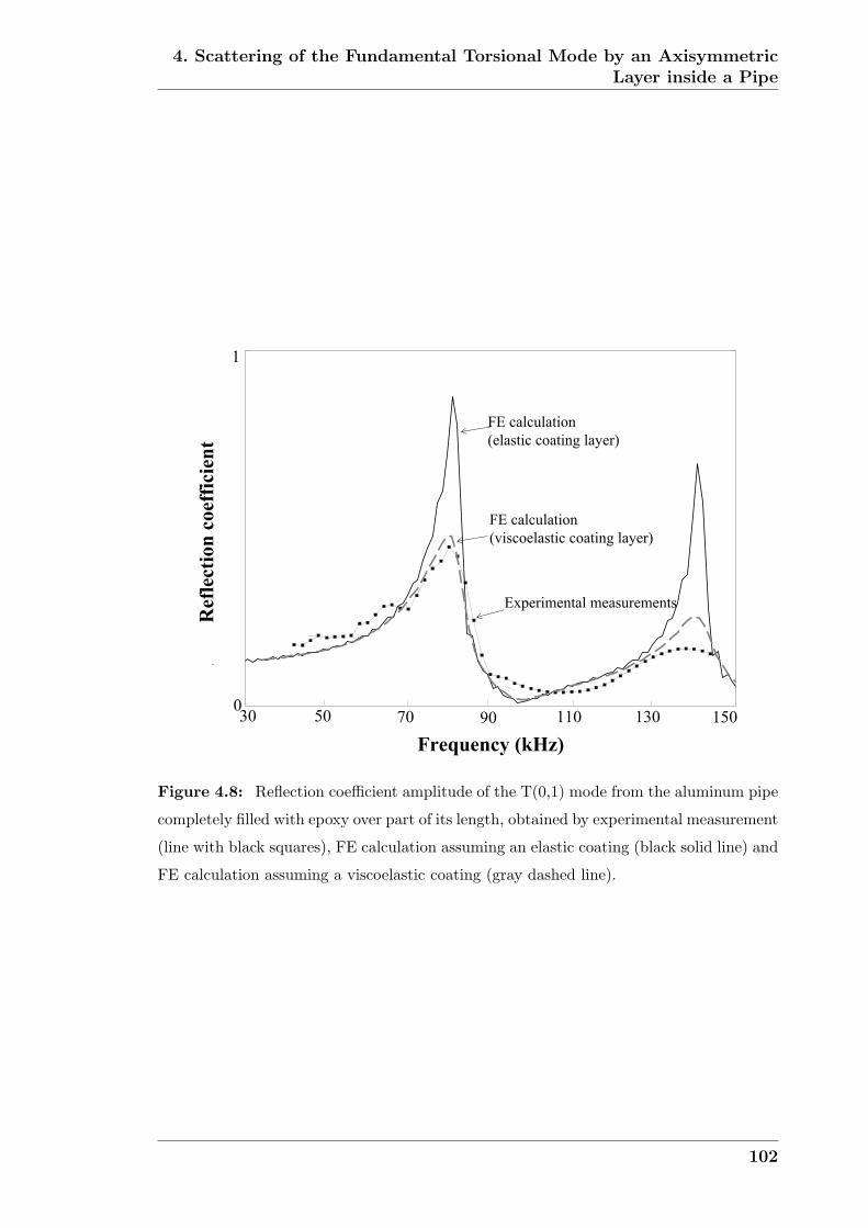
4. Scattering of the Fundamental Torsional Mode by an AxisymmetricLayer inside a Pipe
0
1
FE calculation(elastic coating layer)
FE calculation(viscoelastic coating layer)
Experimental measurements
30 50 70 90 110 130 150
Ref
lect
ion
coef
ficie
nt
Frequency (kHz)
Figure 4.8: Reflection coefficient amplitude of the T(0,1) mode from the aluminum pipe
completely filled with epoxy over part of its length, obtained by experimental measurement
(line with black squares), FE calculation assuming an elastic coating (black solid line) and
FE calculation assuming a viscoelastic coating (gray dashed line).
102

4. Scattering of the Fundamental Torsional Mode by an AxisymmetricLayer inside a Pipe
500
0250 650Time (us)
Freq
uenc
y (k
Hz)
T1
T2
T3
T4
250 650Time (us)Am
plitu
de (A
.U.) (a)
(b)
Figure 4.9: (a) Time-domain signal measured in the bilayered part of the aluminium
pipe locally coated inside with a 6-mm thickness epoxy layer; (b) Reassigned spectrogram
analysis of the measured local signal shown in Fig. 4.9a and analytical calculation (white
dashed lines) by DISPERSE.
103

4. Scattering of the Fundamental Torsional Mode by an AxisymmetricLayer inside a Pipe
Time (us)
Freq
uenc
y (k
Hz)
8000
500
0 T1
T2
T3
T4
Reflection
8000 Time (us)
Am
plitu
de (A
.U.) (a)
(b)
Reflection
Figure 4.10: (a) Time-domain signal measured in the filled part of the aluminium pipe
locally filled with epoxy; (b) Reassigned spectrogram analysis of the measured local signal
and best fit curves (white dashed lines) calculated by DISPERSE for the aluminum pipe
locally filled with epoxy.
104

Chapter 5
Feasibility Study of Sludge and
Blockage Detection inside Pipes
Using Guided Torsional Waves
5.1 Background
The results from Chapter 4, based on the idealised model, have shown the poten-
tial of using the fundamental torsional mode T(0,1) to detect and characterise a
layer inside a pipe; however, the applicability of the two proposed techniques for
the detection of realistic sludge and blockage needs further investigation. This is
obviously due to various practical issues associated with realistic sludge that were
not considered in the idealised model. These issues can significantly complicate the
problem and affect the proposed techniques in different ways. This chapter proceeds
the work by taking into account these more practical issues, including irregular ax-
ial and circumferential profiles of the sludge layer, imperfect bonding state between
the sludge and the pipe and the material damping of the sludge. The purpose is
to investigate how the reflection and transmission techniques are affected by each
of these issues so as to find out the most critical factors and therefore assess the
potential of using guided ultrasonic waves to detect and characterize sludge and
blockages in practice.
105
5. Feasibility Study of Sludge and Blockage Detection inside PipesUsing Guided Torsional Waves
Besides this specific inspection application, the models studied in this chapter are
also linked to models of guided wave propagation in filled waveguides. As reviewed
in previous chapters, a number of models have been conducted to study the effect
of liquid or solid content on the propagation of guided waves [44, 45, 49, 58, 57, 60].
Most of these works assume that the contents are axisymmetric and also have regular
properties along the axial direction. The models considered in this chapter will show
the effect of irregular properties and asymmetric geometry of the contents on the
propagation of the guided waves.
The chapter starts with the model studies of the effects of the irregular properties of
sludge on the two techniques developed in the last chapter (Sec. 5.2). Then results
from a number of experimental measurements are presented in Sec 5.3, including
model experiments for validating the principles and realistic experiments for testing
the practical capabilities. Limitations of the guided wave techniques for sludge
detection and characterization are discussed in Sec. 5.4 and an overall assessment is
given in Sec. 5.5.
5.2 Model Study
The effects of sludge irregularity on the reflection and transmission measurements
are first investigated by FE modeling. A 2D model with the FE software FINEL [85]
was used to study the case in which the sludge layer has an irregular axial profile,
but an axisymmetric circumferential profile. The details of the models are outlined
in Appendix A.1. The dimensions and the material properties of the pipe and the
layer used in the 2D model are the same as those used in the idealised model and
are listed in Table 4.1.
5.2.1 Imperfect bonding state
It is very likely that the bonding between the sludge layer and the pipe is imperfect.
The effect of the bonding state can be studied by using a spring layer model which
has been commonly used to represent imperfect bonding conditions [89]. A fictitious
layer with compressional stiffness KL and shear stiffness KT is inserted between the
106

5. Feasibility Study of Sludge and Blockage Detection inside PipesUsing Guided Torsional Waves
pipe and the sludge as shown in Fig. 5.1. Only the shear stiffness KT will affect the
torsional modes since they only have tangential displacements. The thin fictitious
layer used in the FE simulation is 0.1mm thick and the other parts of the model
are the same as in the idealised case. The decreasing of bonding is simulated by
reducing the shear stiffness of the spring layer. More details of the model can be
found in Appendix A.1.
The dispersion curves of the torsional modes in the bilayered pipe with imperfect
bonding state can be numerically calculated with DISPERSE by treating the inter-
face as a special layer with the properties stated above. Fig. 5.2 shows the group
velocity dispersion curves of the first two bilayered pipe modes for three differ-
ent value of the spring layer stiffness. For comparison the case of perfect bonding
(KT ∈ ∞) is also given. It can be observed that as the stiffness of the bonding
decreases, the cutoffs of the higher order bilayered pipe modes move towards lower
frequencies. A similar trend was found by Lanza di Scalea and Rizzo [90] and Cheng
et al. [91] when comparing the dispersion curves of Lamb waves in two bonded plates
with different degrees of bonding state.
As a result, the peak positions on the reflection coefficient spectrum magnitude
(calculated from the FE simulated signals monitored at the reflection measurement
point in Fig. 5.1) shift to lower frequencies with the decreasing of the bond state,
which is shown in Fig. 5.3a. This implies that in practice, due to the uncertain
bonding state, in order to detect the layer, either a broadband frequency excitation
or a frequency sweep is required to guarantee obtaining a strong reflection from the
layer. However, although this approach could lead to the detection of the sludge,
it is not possible to characterize it by measuring peak positions of the reflection
coefficient spectrum since the degree of bonding is normally uncertain in practice.
The reassigned spectrogram analysis of the transmitted T(0,1) mode ( FE simulated
signal monitored at the transmission measurement point in Fig. 5.1) from an imper-
fectly bonded bilayered pipe (case 2: KT = 0.71GPa/mm) is shown in Fig. 5.3b. It
shows that the layer-induced dispersion of the transmitted signal can still be clearly
revealed if the bonding condition is imperfect. The revealed spectrum is compared
with the numerical calculation by DISPERSE showing excellent agreement. In terms
of characterization, it becomes difficult to extract the properties of the layer (thick-
107

5. Feasibility Study of Sludge and Blockage Detection inside PipesUsing Guided Torsional Waves
ness or shear acoustic velocity) from the dispersion of the transmitted signal, since
the degree of bonding also plays a crucial role in the dispersion of the transmitted
signal.
5.2.2 Varying thickness
In practice, a sludge layer may accumulate gradually along the pipe, which means
its thickness varies along its length. Here we discuss the case in which the layer has
a very gentle thickness change at both ends as illustrated in Fig. 5.4a. The part
where the layer has varying thickness is termed the ’tapered bilayered pipe’; while
the part where the layer has uniform thickness will be referred to as the ’uniform
bilayered pipe’. In this model, we assume a perfect bonding state consistently along
the layer. The details of this model can be found in Appendix A.1.
The time trace signal (Fig. 5.5a) from the FE model monitored at the reflection
measurement point in Fig. 5.4a shows the incident wave (70kHz central frequency
with 5 cycles) on its way to the layered pipe region, and a little reflection from the
layer due to the gentle change of its thickness. With the same excitation, about 30%
reflection can be achieved when the thickness change is abrupt as in the idealised
model (Fig. 4.4b). This implies that the smooth thickness change of the sludge layer
will considerably reduce the strength of the reflection from the layer.
On the other hand, there is more energy of the incident signal transmitted through
the tapered bilayered pipe. The reassigned spectrogram of the transmitted signal
from the FE model monitored at the transmission measurement point in Fig. 5.4a is
given in Fig. 5.5b. It shows that the gentle thickness change of the layer delays the
frequencies which are above the first cutoff frequency of the torsional mode in the
uniform bilayered pipe (indicated by F2 in Fig. 4.2a). The layer-induced dispersion
of the transmitted signal can be revealed at the frequencies below F2.
The torsional modes in the tapered bilayered pipe adapt to the thickness varia-
tion of the layer: their phase velocity and wavenumber change continuously during
propagation, depending on the local thickness. However, as the thickness change of
the layer is very gentle along its length, we can approximately consider the tapered
108

5. Feasibility Study of Sludge and Blockage Detection inside PipesUsing Guided Torsional Waves
bilayered pipe region to be equally divided into a large number of ’local uniform bi-
layered pipes’ whose thickness can be considered uniform over a length of lt (shown in
Fig. 5.4a). Due to the thickness variation of the layer, these local uniform bilayered
pipes have different dispersion curves and accordingly, the cutoff frequencies of the
modes also change according to the thickness of the layer: the thinner the layer is,
the higher the cutoff frequencies tend to be. This is illustrated in Fig. 5.6: the cutoff
frequency of the second mode in the tapered bilayered pipe is plotted as a function
of the thickness of the layer. Since the thickness of the layer changes continuously
from zero to the thickness of the uniform part of the layer, the cutoff frequency of
the second mode T2 in the tapered bilayered pipe decreases monotonically from the
cutoff frequency of the clean pipe mode T(0,2) to F2 which corresponds to the cutoff
for the uniform bilayered pipe.
When the T(0,1) mode containing broadband frequencies is incident on the tapered
bilayered pipe region, the frequencies below F2 can freely pass the tapered bilayered
pipe without encountering any cutoff frequency. However, the frequencies above F2
will inevitably match a cutoff frequency of a certain local tapered bilayered pipe,
from where they will be greatly delayed after propagating for a distance of lt due
to the low propagation velocity at the cutoff. Therefore, the dispersion induced by
the uniform bilayered pipe on the transmitted signal can only be preserved in the
frequency range below the F2.
We should also note that when the thickness change of the layer becomes sharp,
the length lt during which the thickness of the layer can be assumed uniform will
tend to be infinitesimal. In this case, all the frequencies can freely pass the tapered
bilayered pipe region since lt is too short to delay the frequencies even if they match
the cutoff frequencies of the tapered bilayered pipe. So the transmitted signal will
be similar to that in the idealised model.
5.2.3 Varying thickness and varying bonding state
Besides the thickness change, the sludge may simultaneously have a non-uniform
bonding state along its axial profile. We proceed next to model a case in which the
sludge layer has the same thickness variation as in the previous case. Moreover, the
109

5. Feasibility Study of Sludge and Blockage Detection inside PipesUsing Guided Torsional Waves
bonding state varies along the tapered bilayered pipe region as shown in Fig. 5.4b.
This is a very likely scenario in practice due to the non-uniform bonding condition.
A spring layer was used to simulate the imperfect bonding and the stiffness of the
spring layer in the front part (state 1) of the layered pipe is half of the latter part
(state 2). This case was made to study the effect of abrupt bonding change along
the sludge layer. More details of the model can be found in Appendix A.1.
The FE simulated signals monitored at the reflection measurement point (in Fig. 5.4b)
are shown in Fig. 5.7a. It shows the incident wave on its way to the layered pipe
region, and a little reflection from the start of the tapered bilayered pipe due to
the gentle thickness change of the layer. However, a much stronger reflection occurs
from the point where there is an abrupt bonding change, although the change of
thickness of the layer at this point is very gentle. This implies that an abrupt change
in bonding state will result in strong reflections regardless of the gentle thickness
change of the layer. Essentially, bonding state, thickness and even material proper-
ties of the sludge will change the mode shape of the torsional mode, any such change
being the cause of reflection. Therefore, we can expect that the reflection may occur
anywhere along the layer where the layer has an abrupt change of its properties.
The more abrupt these change are, the stronger the reflections will be.
The reassigned spectrogram analysis of the transmitted signal from the FE model
monitored at the transmission measurement point ( Fig. 5.4b) is shown in Fig. 5.7b.
Similar to the previous case, the layer-induced dispersion of the transmission signal
can be revealed below the first cutoff frequency of the torsional mode in the uniform
bilayered pipe region.
5.2.4 Non-symmetric circumferential profile
For the next stage of the FE work, a 3D FE model was developed to study the effects
of the circumferential extent of the layer on both techniques. The pipe studied in
this model is different from the 2D model. A 3 inch aluminium pipe (89mm OD
and 2.5mm wall thickness) coated with a 10-mm thickness epoxy layer was modelled.
The corresponding dispersion curves of the torsional mode in such a pipe is shown in
Fig. 5.8a. The model uses the same material properties as the 2D modelling that are
110

5. Feasibility Study of Sludge and Blockage Detection inside PipesUsing Guided Torsional Waves
listed in Table 4.1. The pipe is 2.5m in length, 0.5m of which is coated with a layer
inside. The layer was modelled to have a constant axial profile (perfect bonding
and uniform thickness), but a non-symmetric circumferential profile as shown in
Fig. 5.9a. Four cases were modelled for different circumferential extents of the layer.
The model was carried out using the FE software ABAQUS [92] and the details of
the 3D model are described in Appendix A.2.
The signals are first monitored at the reflection measurement point in Fig. 5.9a to
receive the incident and reflected T(0,1) mode. The effect of circumferential extent
of the layer on the reflection coefficient amplitude spectrum is shown in Fig. 5.8b.
To validate the 3D FE model, the result obtained for the 100% circumferential ex-
tent case were compared to those calculated from the 2D model in FINEL, showing
excellent agreement. Fig. 5.8b clearly indicates that the reduction of the circum-
ferential extent of the layer decreases the strength of the reflection throughout the
frequency range. However, the frequencies at which strongest reflections occur are
not affected by the circumferential extent of the layer.
The transmitted T(0,1) mode was monitored at the transmission measurement point
in Fig. 5.9a. The reassigned spectrogram analyses of the transmitted T(0,1) mode
from the pipe partially coated with the layer of different circumferential extents, are
shown in Fig. 5.10. The signals coming later are the transmitted signal reflected
from the end of the pipe. When the layer is axisymmetric (100% circumferential ex-
tent), the layer-induced dispersion of the transmitted signal can be clearly revealed
and shows excellent agreement with the analytical calculation by DISPERSE; how-
ever, as the layer becomes non-axisymmetric, the layer-induced dispersion of the
transmitted signal becomes irregular and complex. As the circumferential extent of
the layer reduces, the dispersion of the transmitted T(0,1) mode evolves from the
dispersion curve of the torsional bilayered pipe modes (100% circumferential extent)
to the dispersion curve of the incident T(0,1) mode (non-dispersive). The complex-
ity of the dispersion of the transmitted T(0,1) mode is still a good indicator of the
presence of the sludge compared to the non-dispersive T(0,1) mode in the clean pipe;
however, the complexity of the dispersion makes it difficult to characterize the layer
quantitatively from the measurements.
The 3D FE model was also extended to study a case when the layer has differ-
111

5. Feasibility Study of Sludge and Blockage Detection inside PipesUsing Guided Torsional Waves
ent thickness around the circumference as illustrated in Fig. 5.9b. The layer was
modelled to have a 10-mm thickness part and a 5-mm thickness part, each occupy-
ing 50% circumferential extent. The circumferential profile of the layer is constant
along its length. All the other parameters of the pipe and the layer are the same
as the last model. The reflection coefficient spectrum calculated from the signals
monitored at the reflection measurement point is shown in Fig. 5.11a. For compar-
ison, the reflection coefficient spectra calculated from the two fully bilayered pipe
model (100% circumferential extent) with respectively 10-mm layer thickness and
5-mm layer thickness are also presented. Fig. 5.11a shows that the peaks on the
reflection coefficient spectrum occur at the frequencies where the peaks of the thin
and thick layers would occur if they were present in the pipe separately with full
circumferential extent. This will increase the possibility of detection.
The transmitted T(0,1) mode was monitored at the transmission measurement point
in Fig. 5.9b with its reassigned spectrogram analyses being shown in Fig. 5.11b. It
is clear that the thickness variation of the layer around the circumference increases
the complexity of the dispersion of the transmitted T(0,1) mode.
5.3 Experiments
Model experiments and realistic experiments have also been conducted. The model
experiments were conducted to validate the principles predicted by the FE models.
The setup of the model experiments are the same as described in Chapter 4 (Fig. 4.6).
The model experiments were conducted on two small aluminium pipes (16.5-mm
inner diameter and 1.4-mm wall thickness) coated with layers made of different
materials. Due to manufacturing difficulty, the layers were built at one end of the
pipe rather than in the middle of the pipe.
The same setup for the model experiments was used as the one introduced in Chapter
4 (Fig. 4.6). The reflection measurement and local measurements also followed the
same procedures. The slight difference is that the setup uses more pieces of PZT
elements (six pieces) mounted on the external surface of the pipe for excitation and
samples more waveforms for circumferential averaging. This was done to further
112

5. Feasibility Study of Sludge and Blockage Detection inside PipesUsing Guided Torsional Waves
eliminate the flexural modes at higher frequencies.
5.3.1 Model experiment
The reflection measurement was performed on the aluminum pipe containing an
epoxy circular tube of 16.5-mm external diameter and 4.5-mm inner diameter. The
tube was press-fitted inside the pipe to represent the imperfectly bonded layer. The
pipe was 1.3m in length while the epoxy tube was 0.3m long and placed at one end
of the pipe.
The measured reflection coefficient amplitude spectrum from this sample is shown
in Fig. 5.12. For comparison, we also show the results from a sample of pipe with
a perfectly bonded epoxy layer which was presented in Chapter 4. This was made
by casting the epoxy layer (6mm uniform thickness) inside the pipe. The press-
fit epoxy layer gives reduced contact to the pipe wall compared to the cast epoxy,
which is to represent a poorer bonding condition. The epoxy resin employed for
both cases is a commercial adhesive, Araldite 2020, whose acoustic properties are
listed in Table 4.2.
The FE predictions for both cases are plotted in Fig. 5.12. As shown before, the
measured peak position of the reflection coefficient amplitude spectrum matches very
well with the predicted one in the case of perfect bonding. The agreement for the
imperfect bonding case was achieved by choosing a suitable contact stiffness value in
the FE model. The discrepancy between the modelling and the experiments on the
magnitude of the reflection coefficient spectrum has been known as being caused by
the material damping of the epoxy, which was not considered in the FE modelling.
Most importantly, both measurements and simulations confirm that the imperfect
bonding condition between the layer and the pipe shifts the peaks of the reflection
coefficient amplitude spectrum to lower frequencies.
The local signal was measured on the part of the pipe coated with the imperfectly
bonded layer, at a position 0.05m away from where the layer starts in the pipe. The
reassigned spectrogram analysis of the measured local signal is shown in Fig. 5.13a.
For comparison, the reassigned spectrogram analysis of the incident signal T(0,1)
113

5. Feasibility Study of Sludge and Blockage Detection inside PipesUsing Guided Torsional Waves
measured in the clean pipe region is also given in Fig. 5.13b. It is clear from Fig. 5.13a
that the layer-induced dispersion of the local signal can still be measured when the
bonding of the layer is imperfect. The first two cut-off regions can be identified
where the frequencies are delayed due to the low propagation velocity at the cut-off
frequencies of the bilayered pipe modes.
Measurements were then performed on another sample of pipe coated with an ir-
regularly shaped layer made of simulants of a potential real sludge material shown
in Fig. 5.14. A mixture of Magnesium Hydroxide, Magnesium Oxide and water was
proposed by an industrial partner (Nexia Solutions Ltd) as a useful sludge simulant.
The simulant was transferred into the 1.6-m long pipe to form a 0.4m long sludge
layer. The time trace in Fig. 5.15a is the reflection measurement made at clean pipe
region, 0.8m away from the start of the layer (the reflection measurement point in
Fig. 5.14). It shows the incident signal (30 kHz central frequency with 10 cycles) fol-
lowed by a lower amplitude signal (reflection 1) which is the reflection from the entry
point of the sludge. A much stronger signal (reflection 2) arriving later is reflected
from the middle of the blocked pipe according to its arrival time. Although the
sludge layer has an irregular shape due to the manufacturing difficulty, we believe
that the variation of the thickness of the layer is free from any abrupt change. Thus,
we speculate that this stronger reflection was caused by an abrupt bonding change
of the sludge, since it is hard to guarantee the simulant to have uniform contact with
the pipe when it was transferred into the pipe. The reflection coefficient amplitude
spectra of the reflection 1 and the reflection 2 is shown in Fig 5.15b.
For the transmission measurement, an excitation signal of 150 kHz with 2 cycles was
employed and the measurement was made at a local point in the blocked pipe region
about 0.1m away from where the sludge starts (the transmission measurement point
in Fig. 5.14). The reassigned spectrogram analysis is shown in Fig. 5.16. Instead
of revealing a regular dispersion change as in the last case, the spectrum of the
transmitted signal shows a complex dispersion change of the signal. As shown in
the FE model, this can be caused by the non-symmetric circumferential profile
of the sludge which causes different modes to be generated in the blocked part
of the pipe, with different propagation velocities. Also we noticed that the signal
attenuated quickly as the receiver point was moved further away from the entry point
114

5. Feasibility Study of Sludge and Blockage Detection inside PipesUsing Guided Torsional Waves
of the sludge and became too low to be measured after 0.3 m. Thus, the significant
attenuation of the torsional modes may also be an additional indicator of the sludge,
since the modes propagating in the clean metal pipe have little attenuation over long
distances.
5.3.2 Realistic experiment
To test the applicability of the measurement ideas in practice, a realistic experiment
was performed on a nominal 3 inch (88.9mm OD and 2.5mm wall thickness) steel
pipe using a commercial WaveMaker Pipe Screening system from Guided Ultrasonics
Ltd [93]. The 3-m long pipe was in good condition (no cracks or defects) and had no
welds or flanges. The sludge material was made by mixing Magnesium Hydroxide,
Magnesium Oxide and water in the proportions 54:9:37. The material was then
transferred into the 3 inch pipe to build up the sludge layer which extended up to
1m in length from one end of the pipe. The speculated axial profile is shown in
Fig. 5.17a. Due to the method of manufacturing, the pipe is fully blocked at the
beginning of the sludge for a very short length. The sludge forms a layer with an
estimated average thickness of 15mm for about 0.4m and gradually decreases its
thickness to about 5mm towards the end of the pipe. The pipe was then sealed at
both ends to minimise contact with air and was stored for 14 days to dry before the
tests started. Both reflection measurement and transmission measurements were
carried out at two different times. The first one was conducted immediately after
14 days when sludge was still fairly wet. The second measurements was made one
month after the first one during which the inside of the pipe was open to the air.
This made the sludge become completely dry and solid by the time of the second
measurement.
The setup of the reflection measurement is illustrated in Fig. 5.18a and photographed
in Fig. 5.17c. A Guided Ultrasonics Ltd. transducer ring placed at the outside
surface of the pipe was used to send the T(0,1) mode in both the forward and
backward directions and to receive the reflected signals from any feature in the pipe.
Fig. 5.19a shows a typical reflected signal (25 kHz central frequency with 8 cycles)
from the first measurements when the transducer was placed 1.4m away from the
start of the blocked part of the pipe. The arrival time of the signal was converted to
115

5. Feasibility Study of Sludge and Blockage Detection inside PipesUsing Guided Torsional Waves
distance by measuring the propagation velocity T(0,1) in the clean pipe. The figure
thus shows the amplitude (vertical axis) and the source location (horizontal axis)
of the reflections that can be received by the transducer ring in Fig. 5.18a . The
backward end reflection occurs at -0.6 m, and in the forward direction, there is a
mirroring of the backward end reflection signal at the exact same distance from the
ring. This mirror is known to occur in cases when the reflections in both directions
occur in the near field of the transducer (±1 meter from the ring), because it is not
possible to control the direction of the transmitted and received waves adequately.
In practice, with longer pipes, this problem of mirror signals is avoidable. The
reflection occurring at 1.6m comes from the sludge, but not from the entry point of
the sludge. This may be due to the poor bonding condition at the beginning of the
sludge. Also note that there is little forward end reflection received because of the
large material damping of the sludge.
To calculate the reflection coefficient spectrum, the amplitude of the reflected signal
from the sludge was divided by that of the backward end reflection signal which
can be used to approximate the incident signal. The measured reflection coefficient
obtained from the first experiment is shown in Fig. 5.19b and exhibits a decreasing
trend as the testing frequency increases. A maximum reflection around 17% was
measured at 25 kHz.
The same measurement was repeated one month after the first when the sludge had
become completely dry and solid. The measured reflection coefficient shows very
different frequency dependence from the first measurement as shown in Fig. 5.19b.
A maximum reflection of about 21% can be achieved at 32 kHz. We speculate
that the discrepancy between the two measurements is largely due to the change of
properties of the sludge during the period between the two measurements. As the
sludge becomes more solid, its bonding to the pipe wall improves. This can result
in strong reflections at higher frequencies. Also the material properties may change
as the sludge dries out, which changes its sound velocity. This implies for practical
tests that the frequency range to obtain a strong reflection from sludge may change
significantly as the condition of the sludge changes.
The setup of the transmission measurement is illustrated in Fig. 5.18b and pho-
tographed in Fig. 5.17d. The transmission measurement uses two transducer rings
116

5. Feasibility Study of Sludge and Blockage Detection inside PipesUsing Guided Torsional Waves
working in pitch catch mode: one transducer ring sends the signal which is received
by another one. The excitation employs an excitation signal of 40 kHz central fre-
quency with 3 cycles which covers the frequency band from 20 kHz to 60 kHz. The
guided modes experienced significant attenuation at the time of the first measure-
ments when the sludge was wet. The attenuation caused by the sludge was measured
between 35-40 dB/m which is much stronger than the attenuation caused by any
other feature. A typical site weld is a -14dB [13] reflector and the attenuation caused
by bitumen coating is between 3-10 dB/m [13].
The attenuation of the transmitted signals is much lower at the time of the second
measurements, when the sludge become dry and solid. Both transducer rings were
first placed in the clean pipe region with 1m separation distance. The signal received
by the receiver transducer ring was analyzed by the reassigned spectrogram showing
the non-dispersive T(0,1) mode (Fig. 5.20a). Then the transmitter transducer was
placed in the blocked region keeping the same distance (1 meter) from the receiver
transducer as for the clean pipe (Fig. 5.18b). Its reassigned spectrogram shows the
sludge-induced dispersion of the transmitted signal as some frequencies are delayed
in their arrival time (Fig. 5.20b).
The noise may affect the signal so that the spectrogram may not reveal a strict
non-dispersive signal in the clean pipe as revealed in (Fig. 5.20a). The capability to
identify the sludge-induced dispersion will depend on the noise level. To calibrate
the influence of the noise, it is important to quantify the extent of dispersion of the
signal from the spectrogram. One method to assess dispersion is to calculate the
standard deviation of the arrival time (SDT) of all the frequencies in the received
signal. Figs. 5.21 shows SDT of the signals in Figs. 5.20 a and b respectively,
when different values of threshold are set to extract the dispersion curve from the
spectrogram. The SDT of the signal in the clean pipe (SDTClean) is due to the noise
and ideally it should be zero; the SDT of the signal in the blocked pipe (SDTBlocked)
contains the information about the sludge-induced dispersion. To calibrate sludge-
induced dispersion from the influence of the noise, a ratio of SDT (SDTR) can be
defined as
117

5. Feasibility Study of Sludge and Blockage Detection inside PipesUsing Guided Torsional Waves
SDTR(dB) = 20 log10(SDTBlockedSDTClean
). (5.1)
It can be seen from Figs. 5.21 that the SDTR is always larger than 6dB. In practice, it
will be very useful to identify a threshold of the SDTR from which the sludge induced
dispersion can be reliably detected. This should be achieved through extensive
practical tests to obtain empirical data.
5.4 Discussion
Here we address some issues that will affect the proposed measurements for sludge
and blockage detection in practice.
Firstly, in many circumstances pipes will contain fluid. The proposed measurements
will not be affected by the presence of fluids inside the pipes if they are inviscid such
as water; however, if the fluid is viscous, the torsional mode will have attenuation
which is controlled by the viscosity of the fluid and the operating frequency. This
requires the inspection to use low frequencies to maintain a large testing range.
Secondly, we have shown that it is still possible to detect the sludge if the bonding
is imperfect to a certain extent. However, if the sludge makes a slip contact or is
almost disbonded, then the torsional mode will fail to detect the blockage, since
there is no coupling of guided wave energy between the sludge and the pipe.
Lastly, as we see, the material damping of the sludge or blockage affects the measure-
ments. If the sludge is a highly attenuative material, it may considerably attenuate
the magnitude of both the reflected and transmitted signals. On the other hand,
the large attenuation of the transmitted signal may also be an additional indicator
of presence of the sludge, if the pipe is free from any other attenuative media either
inside or outside.
118

5. Feasibility Study of Sludge and Blockage Detection inside PipesUsing Guided Torsional Waves
5.5 Conclusions
In this chapter we have studied the feasibility of sludge and blockage detection
and characterization using guided torsional waves. Two guided wave techniques
developed from earlier work were advanced by taking into account practical issues
about the sludge, including irregular axial and circumferential profiles of the sludge
layer, imperfect bonding state between the sludge and the pipe and the material
damping of the sludge. The study has investigated the effects of each of these
factors on the two techniques. An overall assessment of the feasibility of sludge
detection and characterisation using guided wave can be summarized as follows.
The reflections of guided ultrasonic waves from sludge can be measured to effectively
locate the sludge in the pipe. The reflection can be caused by any abrupt change
of the properties of the sludge along its axial or circumferential profiles including
bonding state, thickness or material properties. The more abrupt these changes are,
the stronger the reflections will be. The strength of the reflection also enhances
with increasing circumferential extent of the sludge layer. On the other hand, the
material damping of the sludge weakens the strength of the reflection.
The strength of the reflection is frequency dependent. The frequency to obtain
the strongest reflection is determined by the thickness, material properties and the
bonding state. So a practical implementation should sweep the testing frequency
or employ broadband frequency excitation in order to guarantee a strong reflection
from the sludge.
The transmission of guided ultrasonic waves propagating past the blocked pipe re-
gion can be measured to detect the presence of the sludge or blockage, however this
method cannot locate them. The measurement employing a broad band excitation
reveals the sludge-induced dispersion change of the guided waves. The revealed
dispersion may be complex or regular depending on the asymmetry of the sludge
in its circumferential and axial profiles. The transmitted signal may suffer from
large attenuation caused by material damping of the sludge. This may also be an
additional indicator of the presence of the sludge, if the pipe is free from any other
attenuative media either inside or outside.
119

5. Feasibility Study of Sludge and Blockage Detection inside PipesUsing Guided Torsional Waves
For reliable sludge and blockage detection, both the reflection and transmission
measurements should be used since they are two complementary measurements.
For example, when the reflection is weak, most energy of guided wave is transmitted
through the blocked region leading to more sensitive transmission measurements.
Quantification of the extent and material properties of the sludge is difficult because
of their arbitrary shapes and properties. An effective characterisation of the geo-
metrical and material properties of sludge is only possible when the sludge has a
uniform shape and its bonding condition is known.
120

5. Feasibility Study of Sludge and Blockage Detection inside PipesUsing Guided Torsional Waves
Epoxy layerImperfect bonding: spring layer
Reflection measurement Transmission measurementIncident T(0,1) mode
Figure 5.1: Schematic of the model in which the pipe is locally coated with 6-mm
thickness epoxy with an imperfect bonding state.
Frequency (kHz)
Gro
up v
eloc
ity (m
/ms)
12340 2500
3.5
Figure 5.2: Dispersion curves of the first two torsional modes in the pipe coated with
6-mm thickness epoxy layer for different bonding states. Case 1: perfect bonding, shear
stiffness KT ∈ ∞; Case 2: KT = 0.71GPa/mm; Case 3: KT = 0.355GPa/mm; Case 4:
KT = 0.071GPa/mm.
121

5. Feasibility Study of Sludge and Blockage Detection inside PipesUsing Guided Torsional Waves
Time (us)
1
Frequency (kHz)
Ref
lect
ion
coef
ficie
nt
00 250
200 1100
Freq
uenc
y (k
Hz)
0
500
(a)
(b)
1234
Figure 5.3: (a) Reflection coefficient spectrum obtained from FE simulations for the
T(0,1) mode when incident at the region where the pipe is locally coated with 6-mm
thickness epoxy layer, for different bonding states. Case 1: perfect bonding, shear stiffness
KT ∈ ∞; Case 2: KT = 0.71GPa/mm; Case 3: KT = 0.355GPa/mm; Case 4: KT =
0.071GPa/mm; (b)Reassigned Spectrogram analysis of the transmitted signal in the pipe
locally coated with 6-mm thickness epoxy layer with imperfect bonding state (case 2) and
the corresponding numerical calculation with DISPERSE (white dashed curves).
122

5. Feasibility Study of Sludge and Blockage Detection inside PipesUsing Guided Torsional Waves
reyal yxopEo3=θ o3=θ
tnemerusaem noitcelfeR tnemerusaem noissimsnarT
ltlt
lt reyal yxopEepiP
1 etats gnidnoB 2 etats gnidnoB
tnemerusaem noitcelfeR tnemerusaem noissimsnarT
o3=θegnahc gnidnoB
reyal yxopE reyal yxopEo3=θ
)a(
)b(
edom )1,0(T tnedicnI
edom )1,0(T tnedicnI
Figure 5.4: (a) Schematic of the model in which the pipe is locally coated by an epoxy
layer that has varying thickness. The tapered region of the bilayered pipe can be thought
of as a succession of local uniform bilayered pipes; (b) Schematic of the model in which the
pipe is locally coated by an epoxy layer that has varying thickness and varying bonding
state.
123

5. Feasibility Study of Sludge and Blockage Detection inside PipesUsing Guided Torsional Waves
Time (us)
Am
plitu
de (A
.U.)
0 800
Incident signal
Entry reflection
Time (us)
Freq
uenc
y (k
Hz)
1100200
500
0
F2End reflection
(a)
(b)
Figure 5.5: (a) Time trace of the incident and the reflected signals monitored at the
reflection measurement point in Fig. 5.4a; (b) Reassigned Spectrogram analysis of the
transmitted signal monitored at the transmission measurement point in Fig. 5.4a.
124

5. Feasibility Study of Sludge and Blockage Detection inside PipesUsing Guided Torsional Waves
0 0.5 1 1.50
2
4
6
8
F2
T2 cut-off frequency (MHz)
Lay
er th
ickn
ess (
mm
)
Figure 5.6: Cutoff frequency of the second torsional modes in the pipe coated with
epoxy layer as a function of the thickness of the layer.
125

5. Feasibility Study of Sludge and Blockage Detection inside PipesUsing Guided Torsional Waves
Time (us)
Freq
uenc
y (k
Hz)
11000
500
200
Time (us)
Am
plitu
de (A
.U.)
0
Incident signal
Entry reflection
Reflection from bonding change
800
End reflection
(a)
(b)
Figure 5.7: (a) Time trace of the incident and the reflection signals monitored at the
reflection measurement point in Fig. 5.4b; (b) Reassigned Spectrogram analysis of the
transmitted signal monitored at the transmission measurement point in Fig. 5.4b.
126

5. Feasibility Study of Sludge and Blockage Detection inside PipesUsing Guided Torsional Waves
Ref
lect
ion
coef
ficie
nt
0Frequency (kHz)
T(0,1)
T1T2 T3
0 120Gro
up v
eloc
ity (m
/ms)
0
3.5
Frequency (kHz)
(a)
(b)1
2
3
4
1200
1
Figure 5.8: (a) Dispersion curves of the torsional modes in a 3 inch aluminium pipe
coated with 10-mm thickness epoxy layer (black curves) and the T(0,1) mode in the clean
3 inch pipe (gray dashed line); (b) Reflection coefficient amplitude spectrum of the T(0,1)
mode in the 3 inch aluminium pipe coated with 10-mm thickness sludge layer for different
circumferential extents. Case 1: 100% (solid line: 3D model, dotted line: 2D model), Case
2: 75%, Case 3: 50%, Case 4: 25%.
127

5. Feasibility Study of Sludge and Blockage Detection inside PipesUsing Guided Torsional Waves
Incident T(0,1) mode
Reflected T(0,1) modeEpoxy layer
Transmitted T(0,1) mode
Reflection measurement Transmission measurement
Multiple bilayeredpipe modesBilayered pipe region
Epoxy layer Epoxy layerPipe Pipe
(a) (b)
Figure 5.9: (a) Schematic of the model in which the pipe is partially coated with an
epoxy layer that has 50% circumferential extent; (b) Schematic of the model in which the
pipe is coated with an epoxy layer that has 10-mm thickness and 5-mm thickness, each
for 50% circumferential extent.
128

5. Feasibility Study of Sludge and Blockage Detection inside PipesUsing Guided Torsional Waves
Freq
uenc
y (k
Hz)
0
300
450 1150Time (us)
Freq
uenc
y (k
Hz)
0
300
450 1150Time (us)
Freq
uenc
y (k
Hz)
0
300
450 1150Time (us)
75%
50% 25%
450 1150Time (us)
Freq
uenc
y (k
Hz)
0
300 (b)
(c) (d)
Reflection
Reflection Reflection
Reflection
100%(a)
Figure 5.10: (a) Reassigned Spectrogram analysis of the transmitted T(0,1) mode in
the 3 inch pipe partially coated with 10-mm thickness epoxy layer that has 100% cir-
cumferential extent and the corresponding numerical calculation with DISPERSE (white
dashed curves); (b) 75% circumferential extent;(c) 50% circumferential extent ; (d) 25%
circumferential extent.
129

5. Feasibility Study of Sludge and Blockage Detection inside PipesUsing Guided Torsional Waves
0450 1150
Freq
uenc
y (k
Hz)
Time (us)
Reflection
(b)
Ref
lect
ion
coef
ficie
nt
Frequency (kHz)
(a)
200
0 1200
1
Figure 5.11: (a) Reflection coefficient amplitude spectrum of the T(0,1) mode calcu-
lated from the signals monitored at the reflection measurement point in Fig. 5.9. For
comparison, reflection coefficient spectra are also calculated from two cases in which the
layer respectively has 10-mm thickness for 100% circumferential extent (black solid curves)
and 5-mm thickness for 100% circumferential extent (gray solid curves); (b) Reassigned
Spectrogram analysis of the signals monitored at the transmission measurement point in
Fig. 5.9.
130

5. Feasibility Study of Sludge and Blockage Detection inside PipesUsing Guided Torsional Waves
1FE calculation (good bonding)
Experiment (good bonding)
Experiment (imperfect bonding)
0
Ref
lect
ion
coef
ficie
nt
20 150Frequency (kHz)
FE calculation(imperfect bonding)
Figure 5.12: Reflection coefficient amplitude of the T(0,1) mode reflected by a 6-
mm thickness epoxy layer inside an aluminium pipe. Experimental results with perfect
bonding case (line with black squares) and imperfect bonding (line with circles) case. The
reflection coefficient spectra amplitude from FE models for both cases are also provided
for comparison (solid lines).
131

5. Feasibility Study of Sludge and Blockage Detection inside PipesUsing Guided Torsional Waves
50 450Time (us)
50 450Time (us)
Freq
uenc
y (k
Hz)
0
500
Freq
uenc
y (k
Hz)
0
500
First cutoff region
Second cutoff region
(a)
(b)
Figure 5.13: (a) Reassigned Spectrogram of the transmitted signal measured in the
blocked pipe region; (b) Reassigned Spectrogram of the incident signal before the blocked
pipe region.
132

5. Feasibility Study of Sludge and Blockage Detection inside PipesUsing Guided Torsional Waves
Reflection 2Reflection 1
Measurement point 1 Measurement point 2
Simulants of real sludge
End cross section
Incident T(0,1) mode
Figure 5.14: Schematic of the measurements conducted on the pipe with randomly
shaped sludge layer made of simulant representing a real sludge material.
133

5. Feasibility Study of Sludge and Blockage Detection inside PipesUsing Guided Torsional Waves
0 1500Time (us)
Am
plitu
de (A
.U.)
Reflection 1 Reflection 2
Incident signal
20 700
0.3
Frequency (kHz)
Reflection 2
Reflection 1
(b)
Ref
lect
ion
coef
ficie
nt(a)
Figure 5.15: (a) Time trace showing the incident signal and the reflected signals mea-
sured at reflection measurement point in Fig. 5.14; (b) Reflection coefficient spectra mag-
nitude of reflection 1 and reflection 2 in Fig. 5.15a.
134

5. Feasibility Study of Sludge and Blockage Detection inside PipesUsing Guided Torsional Waves
300 9000
500
Time (us)
Freq
uenc
y (k
Hz)
Figure 5.16: Reassigned spectrogram analysis of the local signal measured at transmis-
sion measurement point in Fig. 5.14
135

5. Feasibility Study of Sludge and Blockage Detection inside PipesUsing Guided Torsional Waves
Sludge Layer
Clean Pipe Blocked pipe
(a)
(b)
(c)
(b)
(c) (d)
Figure 5.17: (a) Speculated axial profile of the sludge made up by the simulant of
real sludge in the 3 inch steel pipe; (b) End view photography the blocked pipe with the
sludge layer; (c) The setup of the reflection measurement using commercial WaveMaker
Pipe Screening system to detect the sludge inside the 3.5 inch pipe; (d) The setup of the
transmission measurement.
136

5. Feasibility Study of Sludge and Blockage Detection inside PipesUsing Guided Torsional Waves
Sludge Layer
Incident signal
End reflection
Incident signal
Reflection from sludge End reflection
Transducer ring
(c)
Sludge Layer
Transmission signal
Transducer ring (Receiver) Transducer ring (Transmitter)
(a)
(b)
Figure 5.18: (a) Schematic of the reflection measurements conducted on a 3 inch pipe
with a sludge layer made of simulant of real sludge material, using commercially available
guided wave transducer rings; (b) Schematic of the transmission measurements using a
pair of transducer rings.
137

5. Feasibility Study of Sludge and Blockage Detection inside PipesUsing Guided Torsional Waves
25 500
0.25
Mirroring of backwardend reflection
Reflection from sludge
Forward End reflection
-1 0 1 2 3
Backward end reflection
Transducer position
Distance (m)
Am
plitu
de (A
.U.)
Frequency (kHz)
Ref
lect
ion
coef
ficie
nt(a)
(b)
First measurement
Second measurement
Figure 5.19: (a) Testing result of the reflection measurement conducted on the 3 inch
pipe with sludge using a single commercially available guided wave transducer ring as
shown in Fig. 5.18; (b) Reflection coefficient of the measured reflected T(0,1) mode from
the sludge at two different times (line with stars): first measurement; (line with black
squares): second measurement.
138

5. Feasibility Study of Sludge and Blockage Detection inside PipesUsing Guided Torsional Waves
0 10000
80
Time (us)
Freq
uenc
y (k
Hz)
0 10000
80
Time (us)
Freq
uenc
y (k
Hz)
(a)
(b)
Figure 5.20: (a) Reassigned spectrogram analysis of the transmitted signal conducted
on the clean part of the 3 inch pipe with sludge layer using two guided wave transducer
rings; (b) as in (a) but the measurement were conducted on the blocked part of the pipe.
139

5. Feasibility Study of Sludge and Blockage Detection inside PipesUsing Guided Torsional Waves
0.1 10
20
0
10
Threshold
SDT
(us)
SDT
R (d
B)
SDTBlocked
SDTClean
SDTR
Figure 5.21: Standard deviations of arrival time (SDT) of the signals in Figs. 5.20a
and b (black curves), when different values of threshold are used to extract the dispersion
curves from the reassigned spectrogram. The corresponding ratio (SDTR) is also given
(gray dashed curve).
140

Chapter 6
Feasibility of Sludge and Blockage
Detection inside Pipes using
Guided Longitudinal Waves
6.1 Background
Chapters 4 and 5 presented two techniques using guided torsional waves to detect
and in some cases characterise sludge and blockages inside pipes. This chapter in-
vestigates the feasibility of these two approaches when using the guided longitudinal
waves.
The use of longitudinal modes can be more complicated than torsional waves. Un-
like the T(0,1) which is non-dispersive, the longitudinal modes can be highly or
little dispersive depending on the frequency ranges and the dimension of the pipe.
Therefore, the reflection and the transmission measurements can only be carried out
at limited frequencies where the selected modes exhibit little dispersion. For exam-
ple, Fig. 6.1a shows the group velocity dispersion curves of the longitudinal modes
(labelled as L(0,1) and L(0,2)) in a clean aluminum pipe (16-mm ID, and 1-mm
thickness). For such a pipe, the L(0,1) mode at low frequencies and the L(0,2) mode
at high frequencies have little dispersion and therefore can be used for the measure-
ments (indicated in Fig. 6.1a). Also, the longitudinal modes can actively interact
141

6. Feasibility of Sludge and Blockage Detection inside Pipes usingGuided Longitudinal Waves
with the fluid inside the pipe as shown in Chapters 2 and 3. Thus the measurement
using longitudinal modes can be expected to be highly complicated when fluid is
present inside the pipe.
On the other hand, longitudinal waves couple through a slip interface and therefore
can be more sensitive than torsional waves when the shear coupling is low.
The purpose of the study in this chapter is to assess the feasibility of an approach
based on longitudinal guided waves and to compare it with the torsional wave tech-
niques discussed in Chapters 4 and 5.
The investigation starts with the same idealised model used in Chapter 4 in which the
layer is simplified in terms of geometry, material and bonding state. The dispersive
characteristics of guided longitudinal modes propagating in such a bilayered pipe
are presented in Sec. 6.2, followed by an analysis of the reflection and transmission
techniques based on FE simulations in Sec. 6.3. The effects of irregular properties
of the layer on the measurements are studied in Sec. 6.4. In Sec. 6.5, the study is
expanded to discuss the case when a fluid is present inside the pipe. Experimental
results are presented in Sec. 6.6. Finally, the advantages and disadvantages of the
guided longitudinal wave approach versus the torsional one are discussed in Sec. 6.7.
6.2 Longitudinal Modes in the Bilayered Pipe
Let us consider an aluminium pipe (Inner diameter 16mm and thickness 1.4mm)
coated with an axisymmetric epoxy layer that has uniform 5-mm thickness. Fig. 6.1a
shows the group velocity dispersion curves of the longitudinal modes in such a
bilayered pipe (labelled as L1, L2.... L6) as well as the modes in the clean pipe
(labelled as L(0,1) and L(0,2)). The material the pipe and the coating layer are
summarized in Table 6.1.
Fig. 6.1a shows that the presence of the layer increases the number of the modes of
the clean pipe and causes strong dispersion. For example, at low frequencies, the
L1 mode is much more dispersive than the L(0,1) mode. At high frequencies the
the modes of the bilayered pipe are very complex and dispersive, unlike the L(0,2)
142

6. Feasibility of Sludge and Blockage Detection inside Pipes usingGuided Longitudinal Waves
Table 6.1: Material properties used for DISPERSE calculations and FE simulations.
Longitudinal velocity(m/s) Shear velocity(m/s) Density(kg/m3)
Aluminium 6320 3130 2700
Epoxy 2610 1100 1170
Water 1500 1000
mode of the free pipe which has little dispersion.
The longitudinal modes in the bilayered pipe originate from the interaction between
the modes of the clean pipe and those of the equivalent layer if it were rigidly clamped
at the bilayer interface [52]. Therefore, the dispersion characteristics of the modes
in the bilayered pipe are greatly determined by the longitudinal bulk velocity, the
shear bulk velocity and the thickness of the coating layer. However, it is interesting
to find that at low frequencies, the L1 mode is little affected by the longitudinal
bulk velocity of the layer, while it is only determined by the shear bulk velocity and
the thickness of the layer. This is shown in Fig. 6.1b.
6.3 Scattering of the Longitudinal Modes: Ide-
alised Model
The scattering of the longitudinal modes by the idealised layer is studied as in the
case of torsional waves (shown in Fig. 4.1). Instead of using the T(0,1) mode, a
longitudinal mode is incident from the free end of the pipe. At the discontinuity,
the incident mode is partly reflected back into the free pipe (reflected signal), and
also partly transmitted into the longitudinal modes in the bilayered pipe and then
further converted back into the modes of the clean pipe after the bilayered region
(transmitted signal). A 2D FE model is used to model the scattered signals of the
longitudinal modes in such a structure, using the FE software ABAQUS [92]. Its
details are summarized in Appendix B.1.
143

6. Feasibility of Sludge and Blockage Detection inside Pipes usingGuided Longitudinal Waves
6.3.1 Reflection measurement
The reflection measurement uses both the L(0,1) mode and the L(0,2) mode at
plateau regions on their dispersion curves. The incident and the reflected longitu-
dinal modes from the FE simulation are monitored in the reflection measurement
point in Fig. 4.1 to calculate the reflection coefficient spectrum amplitude. This is
shown in case 1 of Fig. 6.2a when the L(0,1) mode is incident and Fig. 6.2b when
the L(0,2) mode is incident. The behavior of the reflection coefficient spectrum
amplitude can be explained by examining the energy flow distribution of guided
longitudinal waves in the bilayered pipe. The parameter of energy flow ratio (EFR)
is similarly defined as the ratio of the energy flow in the pipe to that in the layer
and is plotted in Fig. 6.3 as a function of frequency.
When the the L(0,1) mode is incident at low frequencies, only L1 is present in the
bilayered pipe. Thus the magnitude of the reflected L(0,1) mode uniquely depends
on the EFR of the L1 mode which shows a decreasing trend until a minimum as
frequency increases (Fig. 6.3). This correspondingly increases the mismatch of the
energy flow mode shapes between the L(0,1) mode and the L1 mode and therefore
results in an increasing reflection. As the EFR of the L1 mode at low frequencies
is only determined by the shear bulk velocity and the thickness of the layer, the
reflection coefficient spectrum amplitude also only depends on these two parameters
while it is independent of the longitudinal bulk velocity of the layer. Once the
reflection coefficient spectrum is experimentally measured, it is possible to obtain
the thickness of the layer by a best-fitting procedure, provided that the shear bulk
velocity is known, and vice versa.
The situation becomes more complex when the L(0,2) mode is incident at high
frequencies where there are multiple longitudinal modes present in the bilayered
pipe. The magnitude of the reflection depends on the energy flow mode shapes of
all the modes present in the bilayered pipe weighed by their transmittability from
the incident L(0,2) mode. The peak of the reflection coefficient spectrum amplitude
in Fig. 6.2b approximately occurs at the frequency where the EFR of all the present
modes in the bilayered pipe reaches a local minimum such as the one indicated as
f0 in Fig. 6.3. This frequency is now determined by the longitudinal bulk and shear
velocities and the thickness of the layer.
144

6. Feasibility of Sludge and Blockage Detection inside Pipes usingGuided Longitudinal Waves
Besides the reflected L(0,2) mode, there is also a reflected L(0,1) mode that is
mode-converted from the incident L(0,2) mode at the discontinuity. However, the
reflected L(0,1) mode is much weaker than the reflected L(0,2) mode. The approach
to separate the L(0,1) mode with the L(0,2) mode in FE simulation is described in
Appendix B.1.
6.3.2 Transmission measurement
The transmission measurement reconstructs the layer-induced dispersion from the
transmitted longitudinal modes. A broadband longitudinal excitation (100 kHz
central frequency with 2 cycles) is applied at one end of the clean pipe in its axial-
direction. At low frequencies, L(0,1) is the only mode to be generated and at higher
frequencies, the L(0,2) mode is dominantly excited compared to the L(0,1) mode
due to the match of its mode shape displacement with the excitation. This can be
seen in Fig. 6.4a, the reassigned spectrogram of the FE simulated signals monitored
at the transmission measurement point in Fig. 4.1 for the clean pipe.
The transmitted longitudinal modes propagating past the bilayered pipe is moni-
tored at the transmission measurement point in Fig. 4.1 and its reassigned spec-
trogram analysis is shown in Fig. 6.4b. The numerical calculation is obtained with
DISPERSE showing excellent agreement. The presence of the layer changes the
dispersion of the transmitted longitudinal modes. The most dramatic dispersion
change occurs for the L(0,2) mode, which has little dispersion after its cutoff region
in the clean pipe as shown in Fig. 6.4a. The change of dispersion depends on the
four parameters of the layer: the longitudinal and shear bulk velocities, the thick-
ness and the length; however, for the transmitted L(0,1) mode, the longitudinal bulk
velocity does not effect the dispersion. It should be noted that there is a spike on the
dispersion curves calculated by DISPERSE. This is due to the intersection of two
neighboring modes and their velocities reach a local minima at a very narrow fre-
quency range. However, the reassigned spectrogram cannot represent this frequency
range due to the resolution limit.
145

6. Feasibility of Sludge and Blockage Detection inside Pipes usingGuided Longitudinal Waves
6.4 Irregular Properties of the Layer
The effects of irregular properties of the layer on the reflection and transmission mea-
surements are also studied. A 2D model was used with the FE software ABAQUS to
study the case in which the layer has an irregular axial profile, but an axisymmetric
circumferential profile. The details of the models are outlined in Appendix B. The
dimensions and the material properties of the pipe and the layer used in the model
are the same as those used in the idealised model and are listed in Table 6.1.
6.4.1 Imperfect bonding state
The effect of the bonding state is also simulated by inserting a spring layer between
the pipe and the layer consisting of one spring perpendicular to the bilayer interface
with compressional stiffness KN and another along the interface in the axial direction
with shear stiffness KT . The decreasing of bonding is simulated by reducing both
stiffnesses. More details of the model can be found in Appendix B.2.
The effects of the imperfect bonding on the reflection coefficient spectrum amplitude
(calculated from the FE simulated signals monitored at the reflection measurement
point in Fig. 5.1) are respectively shown in Fig. 6.2a for the cases of the L(0,1)
mode incident and Fig. 6.2b for the case of the L(0,2) mode incident. At low
frequencies when the L(0,1) mode is incident, the imperfect bonding just shifts
the peak positions of the reflection coefficient amplitude spectrum towards lower
frequencies. The similar effect is observed when L(0,2) is incident. It is also clear
that the poor bonding state significantly reduces the magnitude of the reflection at
high frequencies.
The reassigned spectrogram analysis of the FE simulated transmitted signals from an
imperfectly bonded bilayered pipe (case 2: KT = 0.71GPa/mm) is shown in Fig. 6.5,
as well as the numerical calculation by DISPERSE (dashed curves). Compared to
Fig. 6.4b (perfect bonding case), it shows that the the bonding also changes the
dispersion of the transmitted longitudinal modes.
An extreme condition of the imperfect bonding, commonly referred to as ’slip bond-
146

6. Feasibility of Sludge and Blockage Detection inside Pipes usingGuided Longitudinal Waves
ing’ [94], is also considered here. For such a bonding, the compressional stiffness
of the spring layer KN approaches infinity and the shear stiffness KT approaches
zero. So the energy coupling between the pipe and the layer is mainly through the
radial displacement of a guided wave mode. In this case, torsional modes would be
insensitive to the presence of the layer.
The dispersion curves of the longitudinal modes in the bilayered pipe with a slip
bonding are shown in Fig. 6.6a (calculated with DISPERSE). The modes in the
clean pipe are also given for comparison.
Fig. 6.7a shows a time-trace signal of the reflection measurement, when the L(0,1)
mode is incident at low frequencies (50 kHz central frequency with 5 cycles). The
slip bonding is assumed between the pipe and the layer. It shows that there is
little signal reflected by the layer. This is due to the fact that at low frequencies,
the L1 mode has dominant axial displacement compared to the radial displacement.
This is shown in Fig. 6.6b. The energy of the mode is coupled into the layer only
thorough its radial displacement. Therefore, the energy flow mode shape of the L1
mode is predominantly in the pipe wall matching well the incident L(0,1) mode and
no strong reflection can occur.
The reassigned spectrogram analysis of the transmitted longitudinal modes from
the bilayered pipe with the slip bonding is shown in Fig. 6.6b. The transmission
measurement is still capable to reveal the layer-induced dispersion on the transmit-
ted signals for the slip bonding. The comparison with numerical calculations by
DISPERSE (dashed curves) shows a very good agreement.
6.4.2 Varying thickness and bonding state
The effects of varying thickness and bonding state are also studied. The details of
this model can be found in Appendix B.3.
Fig. 6.8 shows FE simulated time-trace signals of the reflection measurement when
the L(0,1) mode is incident at low frequencies (50 kHz central frequency with 5
cycles). In the case of Fig. 6.8a, the layer has a gentle change of thickness and
consistent perfect bonding (shown in Fig. 5.4a); while in the case of Fig. 6.8b, the
147

6. Feasibility of Sludge and Blockage Detection inside Pipes usingGuided Longitudinal Waves
layer has the same change of thickness but an abrupt change of bonding in the middle
of the tapered bilayered pipe region (shown in Fig. 5.4b). The smooth change of
thickness of the layer considerably reduces the strength of the reflection by the layer,
but the abrupt change of bonding state can still result in large reflections.
Correspondingly, the FE simulated transmitted signals monitored at the transmis-
sion measurement points in the two models are processed by the reassigned spectro-
gram. Fig. 6.9a shows that the very gentle change of thickness of the layer delays
the frequencies which are above the first cutoff frequency of the longitudinal mode
in the uniform part of the bilayered pipe. The layer-induced dispersion therefore can
be revealed from the transmitted L(0,1) mode when comparing the reconstructed
spectrum with dispersion of the L(0,1) mode when the layer is not present (white
dashed curve calculated with DISPERSE). The interpretation of such phenomena
can follow the one given in Chapter 5 for the case of the torsional modes. When the
layer has varying thickness and inconsistent bonding, the transmitted longitudinal
modes show complex dispersion as shown in Fig. 6.9b.
6.5 Presence of Fluid inside the Pipe
It has been discussed in Chapter 5 that the presence of inviscid fluid inside the pipe
has no influence on the proposed two measurements when using the guided torsional
waves. However, such fluids can significantly complicate the same measurements
when using the longitudinal waves. It has been shown in Chapters 2 and 3 that the
longitudinal modes can actively interact with the fluid and behave differently from
the modes in the clean pipe.
The model used to study the effect of fluid is illustrated in Fig. 6.10. The pipe and
the layer are modelled to be the same as those in Sec 6.3; additionally, the pipe
is filled with water. The region of pipe filled with fluid is denoted as ’water-filled
pipe’ and the region when the layer is present is termed as ’water-layer pipe’. The
group velocity dispersion curves of the longitudinal modes in the water-filled pipe
(labeled as Lw1 , Lw2 ,Lw3 and Lw4 ) and modes in the water-layer pipe (labeled as Lw−l1 ,
Lw−l2 ....Lw−l6 ) are shown in Fig 6.11. The material properties of the pipe, water and
148

6. Feasibility of Sludge and Blockage Detection inside Pipes usingGuided Longitudinal Waves
the layer are summarized in Table 6.1.
The dispersion curves of the longitudinal modes in the water-filled pipe exhibit
plateau regions and branching regions as observed in Chapters 2 and 3. Due to these
dispersion characteristics, the reflection measurement can only be carried out at the
plateau regions of each mode, where the mode exhibits little dispersion. For example,
Fig. 6.12 shows time-trace signals monitored at the reflection measurement point in
Fig. 6.10, when the plateau regions of the Lw1 mode and the Lw4 mode are individually
chosen as the incident mode (see dashed loops in Fig 6.11). The magnitude of the
reflection by the layer depends on the extent of the mismatch of the energy flow
mode shapes between the incident water-filled pipe modes (at plateau region, the
mode shape is dominant in the pipe wall) and the modes in the water-layer pipe.
The transmission measurement uses a broadband excitation (100 kHz central fre-
quency with 2 cycles) to generate the modes in the water-filled pipe, and the trans-
mitted signal is monitored at the transmission measurement point in Fig. 6.10.
Assuming that at each frequency, one mode in the water-filled pipe is dominantly
present, the transmitted signals in Fig. 6.10 can be expressed as
U(ω) = U0(ω)eikw(L−l)N(ω)∑J=1
TwlJ (ω)T lwJ (ω)eikJ(w−l)l, (6.1)
where, U0 is the amplitude of the excitation signal, ω is the angular frequency and
N(ω) is the number of longitudinal modes in the water-layer pipe at the frequency
ω. kw = ωCw(ω)
, kJ(w−l) = ωCJ(w−l)(ω)
. Cw(ω), CJ(w−l)(ω) are the phase velocity of the
modes propagating in the water-filled pipe, and in the water-layer pipe respectively.
TwlJ (ω) is the transmission coefficient from the incident water-filled pipe mode into
the Jth water-layer pipe mode, whereas T lwJ (ω) is the transmission coefficient from
the Jth water-layer pipe mode to the transmitted water-filled pipe mode. L denotes
the total length between the transmitter and the receiver and l is the length of the
water-layer pipe region.
As the modes in both the water-filled pipe and the water-layer pipe are dispersive,
149

6. Feasibility of Sludge and Blockage Detection inside Pipes usingGuided Longitudinal Waves
the dispersion of the transmitted signal depends on the factor eikJ(w−l)l in the water-
layer pipe and the factor eikw(L−l) in the water-filled pipe. To identify the dispersion
change induced by the layer, a ratio L−ll
, the length of the unblocked region be-
tween the transmitter and receiver to that of the blocked region plays an important
role. When the ratio is small, the change of dispersion due to the layer can be
clearly identified from the transmitted signal. This is shown in Fig. 6.13a, which
is the reassigned spectrogram analysis of the transmitted signal when the length
of the water-filled region is 3 times that of the water-layer region. The numerical
calculation is provided by DISPERSE showing excellent agreement.
However, when L−ll
is large, the dispersion change due to the layer is too subtle
to be appreciated from the transmitted signal. This is shown in Fig. 6.13b, the
reassigned spectrogram of the transmitted signal monitored in Fig. 6.10 when the
length of the water-filled region is 10 times that of the water-layer region. The
represented dispersion curves of the transmitted signal are very close to those of
the water-filled modes. This implies that the capability of remote detection by the
transmission measurement is impaired by the presence of the water when using the
guided longitudinal waves.
6.6 Experiments
Experiments have also been carried out to demonstrate the use of the longitudinal
modes. The experimental setup is illustrated in Fig. 6.14 and is similar to the one
used for the torsional mode experiment; however, different excitation and receiving
methods are used. In order to generate longitudinal modes, a commercial longitudi-
nal transducer (Panametrics, 200 kHz central frequency) is fixed at one end of the
pipe by a transducer holder to generate longitudinal vibration in the axial direction
of the pipe. The axial displacements of the modes propagating in the pipe is re-
ceived by focusing the two beams at 30o with respect to the radial direction and by
orienting the beams in the plane parallel to the axis of the pipe. Waveforms were
sampled at eight equally spaced points around the circumference of the pipe at the
same axial location. By adding the eight sampled waveforms, the flexural modes
can be cancelled by circumferential averaging.
150

6. Feasibility of Sludge and Blockage Detection inside Pipes usingGuided Longitudinal Waves
The sample of pipe consists of a 1.6-m long aluminum pipe (14-mm inner diameter
and 1-mm wall thickness), 0.25m of which contains an epoxy circular tube of 14-mm
external diameter starting from one end of the pipe. The epoxy tube is manufactured
to be axisymmetric, but has a varying thickness along the pipe axis. It is tapered
at both ends for 0.075 m, but keeps a uniform thickness in the middle part (5-mm
thickness) for 0.1 m. The tube was press-fitted inside the pipe, so its bonding with
the pipe wall is imperfect. The epoxy resin employed is the Araldite 2020, whose
acoustic properties were listed in Table 4.2.
The reflection measurement has been carried out at the clean pipe region 0.68m
away from the start of the epoxy tube. Both L(0,1) mode and L(0,2) mode are
used as the incident mode. Fig. 6.15a shows the the measured reflection coefficient
amplitude spectrum from the sample when the L(0,1) mode at low frequencies is
incident. The strong reflection from a layer with tapered interface is anomalous.
However by closely examining the arrival time of the reflected signal, it was found
that the reflected signal actually occurs at a position 0.1m away from the start of
the epoxy tube which is in the uniform part of the layer. This implies that the
contact between the layer and the pipe is inconsistent along the layer.
Fig. 6.15b shows a time-trace signal monitored at the same position when the L(0,2)
mode (180 kHz central with 10 cycles) is incident. Little reflection from the the epoxy
layer can be measured. This confirms the FE predictions that the the imperfect
bonding significantly reduces the magnitude of the reflections at high frequencies.
The principle of the transmission measurement is demonstrated by a local measure-
ment. A broadband longitudinal excitation is used (250 kHz central frequency with
2 cycles) and the local signal is measured on the layered part of the pipe, 0.12m
away from where the layer starts in the pipe. The reassigned spectrogram analysis
of the measured local signal is shown in Fig. 6.16a. The reassigned spectrogram
analysis of the incident longitudinal modes measured in the clean part of the pipe is
also given in Fig. 6.16b. The dispersion changes on both the L(0,1) mode and the
L(0,2) mode induced by the layer can be clearly identified.
151

6. Feasibility of Sludge and Blockage Detection inside Pipes usingGuided Longitudinal Waves
6.7 Conclusions
This Chapter has investigated the feasibility of using guided longitudinal waves to
detect and characterise sludge and blockages inside pipes. It is a generalization
of the two techniques developed in Chapters 4 and 5 which used guided torsional
waves.
It has been shown through the FE simulations and experiments that both reflec-
tion and the transmission measurements can employ guided longitudinal waves to
detect presence of the sludge and blockages inside pipes, although characterisation
is difficult. Both measurements need to be carried out at suitable frequency ranges
on the dispersion curves of the chosen longitudinal modes, where they exhibit little
dispersion.
An advantage of using guided longitudinal waves is that they can interact with the
layer through both the normal and the shear stiffnesses of the interface. Therefore,
techniques using longitudinal modes are more likely to lead to a successful detection
when the bonding interface has small shear stiffness, such as in the case of slip
bonding.
On the other hand, compared to the measurements based on torsional waves, the
longitudinal waves can only be used in limited frequency ranges where the modes
have little dispersion. This reduces the possibility of detection. However, this prob-
lem is less severe for larger pipes in which the L(0,2) mode has little dispersion in
the most commonly used frequency range (20 kHz to 70 kHz) for practical tests.
The presence of fluid inside the pipe severely affects the measurement using the
longitudinal modes. For example, the test frequency range for the reflection mea-
surement is further limited and the remote detection capability of the transmission
measurement is significantly impaired. Therefore, for such situation, torsional waves
should be used instead of longitudinal waves.
152

6. Feasibility of Sludge and Blockage Detection inside Pipes usingGuided Longitudinal Waves
L1
L3
L(0,1)
L4L5
L(0,2)
L2 L6300Frequency (kHz)
Gro
up v
eloc
ity (m
/ms)
0
6
0
100Frequency (kHz)0
Gro
up v
eloc
ity (m
/ms)
6
0
L1
(a)
(b)
Figure 6.1: (a) Group velocity dispersion curves of the longitudinal modes in an alu-
minum pipe (Inner diameter 16mm and thickness 1.4mm) coated with a 5-mm thickness
epoxy layer inside (black solid curves). For comparison, the longitudinal modes in a
pipe without coating are also shown (dashed curves). Material properties are given in
Table 6.1. (b) Dispersion curves of the L1 mode for different bulk velocities. Bulk longi-
tudinal velocity Cl = 2610m/s and bulk shear velocity Cs = 1100m/s (black solid curve);
Cl = 2610m/s and Cs = 1000m/s (gray dashed curve); Cl = 4000m/s and Cs = 1100m/s
(black dotted curve).
153

6. Feasibility of Sludge and Blockage Detection inside Pipes usingGuided Longitudinal Waves
65Frequency (kHz)35
300Frequency (kHz)200
0
1R
efle
ctio
n co
effic
ient
0
1
Ref
lect
ion
coef
ficie
nt(a)
(b)
123
1
23
Figure 6.2: (a) Reflection coefficient spectrum obtained from FE simulations, when
the L(0,1) mode is incident at the region where the pipe is locally coated with 5-mm
thickness epoxy layer, for different bonding states. Case 1: Perfect bonding ; Case 2:
KN = 5GPa/mm, KT = 1.4GPa/mm; Case 3: KN = 2.5GPa/mm, KT = 0.7GPa/mm.
(b) As a, but for the case when the L(0,2) mode is incident.
154

6. Feasibility of Sludge and Blockage Detection inside Pipes usingGuided Longitudinal Waves
Frequency (kHz) 30000
16
Ene
rgy
flow
rat
io
L1 L2
L3 L4
L5
L6
f0Figure 6.3: (a) Energy flow ratio (FER) of the longitudinal modes in Fig. 6.1a.
155

6. Feasibility of Sludge and Blockage Detection inside Pipes usingGuided Longitudinal Waves
Freq
uenc
y (k
Hz)
0
500
250 600Time (us)
(b)
500Fr
eque
ncy
(kH
z)
0250 600Time (us)
(a)
Reflection
Figure 6.4: (a) Reassigned spectrogram analysis of the FE simulated transmitted signals
monitored at the transmission measurement point in Fig. 4.1, assuming the layer is not
present. (b) Reassigned spectrogram analysis of the FE simulated transmitted signals
monitored at the transmission measurement point in Fig. 4.1. The comparisons with
numerical calculations (white dashed curves) is provided by DISPERSE.
156

6. Feasibility of Sludge and Blockage Detection inside Pipes usingGuided Longitudinal Waves
500
Freq
uenc
y (k
Hz)
0250 600Time (us)
Figure 6.5: Reassigned spectrogram analysis of the FE simulated transmitted sig-
nals of longitudinal modes monitored at the transmission measurement point in Fig. 5.1
(KN = 5GPa/mm, KT = 1.4GPa/mm) and the corresponding numerical calculation
with DISPERSE (white dashed curves).
157

6. Feasibility of Sludge and Blockage Detection inside Pipes usingGuided Longitudinal Waves
300Frequency (kHz)
Gro
up v
eloc
ity (m
/ms)
6
00
L(0,1) L(0,2)
L1
L3 L4L5
L2(a)
89
Rad
ial p
ositi
on (
mm
)
Epoxy
Pipe wall
0Amplitude (A.U.)
3 (b)
A
Figure 6.6: (a) Group velocity dispersion curves of the longitudinal modes (black solid
curves) in an aluminum pipe coated with a 5-mm thickness epoxy layer inside. A slip
bonding is assumed at the bilayer interface. The modes in the corresponding free pipe are
also given (gray dashed curves); (b) Displacement mode shape at point A (solid line) axial
displacement; (dashed line) radial displacement.
158

6. Feasibility of Sludge and Blockage Detection inside Pipes usingGuided Longitudinal Waves
0 600Time (us)
Am
plitu
de (A
.U.)
500
Freq
uenc
y (k
Hz)
250 600Time (us)0
Incident L(0,1)
Reflected L(0,1)
(a)
(b)
Figure 6.7: (a) Time-trace signals of the incident and the reflected signals monitored
at the reflection measurement point in Fig. 5.1, when the slip bonding is assumed. The
L(0,1) mode is selected as the incident mode; (b) Reassigned Spectrogram analysis of the
transmitted signal monitored at the transmission measurement point in Fig. 5.1.
159

6. Feasibility of Sludge and Blockage Detection inside Pipes usingGuided Longitudinal Waves
0 600Time (us)
Am
plitu
de (A
.U.)
Incident signal
Entry reflection
0 600Time (us)
Am
plitu
de (A
.U.)
Incident signal
Entry reflection
Reflection due to the bonding change
(a)
(b)
Figure 6.8: (a) Time-trace signals of the incident and the reflected signals monitored at
the reflection measurement point in Fig. 5.4a, when the L(0,1) mode is incident; (b) Time
trace of the incident and the reflected signals monitored at the reflection measurement
point in Fig. 5.4b, when the L(0,1) mode is incident.
160

6. Feasibility of Sludge and Blockage Detection inside Pipes usingGuided Longitudinal Waves
500Fr
eque
ncy
(kH
z)
250 600Time (us)0
500
Freq
uenc
y (k
Hz)
250 600Time (us)0
(a)
(b)
Transmitted L(0,1) in the clean pipe
Figure 6.9: (a) Reassigned Spectrogram analysis of the transmitted signal monitored
at the transmission measurement point in Fig. 5.4a, using the longitudinal modes for
incidence. The numerical calculation of the dispersion curve of the L(0,1) mode in the clean
pipe is also provided by DISPERSE (white dashed curve);(b) Reassigned Spectrogram
analysis of the transmitted signal monitored at the transmission measurement point in
Fig. 5.4b, using the longitudinal modes for incidence.
161

6. Feasibility of Sludge and Blockage Detection inside Pipes usingGuided Longitudinal Waves
Incident signal
Reflected signal Transmitted signal
Reflection measurement Transmission measurement
Water-layer pipe region
Water Water
Pipe
Epoxy
Figure 6.10: Schematic of the model in which an aluminum pipe (Inner diameter 16mm
and thickness 1.4mm) is filled with water and also is locally coated by a 5-mm thickness
epoxy layer.
Lw1
Lw2
Lw3Lw4
Lw-l1
Lw-l2 Lw-l3
Lw-l4 Lw-l5
Lw-l6300Frequency (kHz)
Gro
up v
eloc
ity (m
/ms)
6
00
Figure 6.11: Dispersion curves of the longitudinal modes in the water-filled pipe (gray
dashed curves) and the longitudinal modes in the water-layer pipe (black solid curves).
162

6. Feasibility of Sludge and Blockage Detection inside Pipes usingGuided Longitudinal Waves
0 600Time (us)
Am
plitu
de (A
.U.)
Incident Lw3 Mode
Reflected Lw3 Mode
Incident Lw1 Mode
Reflected Lw1 Mode
0 600Time (us)
Am
plitu
de (A
.U.)
(a)
(b)
Figure 6.12: (a) Time-trace signals of the incident and the reflected signals monitored
at the reflection measurement point in Fig. 6.10, when the Lw1 mode at its plateau region
is used for incidence; (b) For the case when the Lw4 mode at its plateau region is used for
incidence.
163

6. Feasibility of Sludge and Blockage Detection inside Pipes usingGuided Longitudinal Waves
500Fr
eque
ncy
(kH
z)
0250 600Time (us)
(a)
500
Freq
uenc
y (k
Hz)
250 600Time (us)0
(b)
Figure 6.13: (a) Reassigned Spectrogram analysis of the transmitted signal monitored
at the transmission measurement point in Fig. 6.10, when the length of the water-filled
region is 3 times that of the water-layer region. The numerical calculation is also provided
by DISPERSE (white dashed curve);(b) as (a), for the case, when the length of the water-
filled region is 10 times that of the water-layer region.
164

6. Feasibility of Sludge and Blockage Detection inside Pipes usingGuided Longitudinal Waves
Receive point of reflected signal
Free Pipe
Differential optical sensor head
Displacement and velocity decoder
Digital Oscilloscope
Waveform generator
Receive point oflocal signal
Longitudinal transducer
PC
Imperfect bondingEpoxy layer
Figure 6.14: Schematic of the experiment measurements conducted on a pipe locally
containing an epoxy tube that has varying thickness and imperfect bonding state.
165

6. Feasibility of Sludge and Blockage Detection inside Pipes usingGuided Longitudinal Waves
40 70Frequency (kHz)
Ref
lect
ion
coef
ficie
nt
0
1
90 280Time (us)
Am
plitu
de (A
.U.)
Incident L(0,2) Mode
(a)
(b)
Figure 6.15: (a) Reflection coefficient spectrum amplitude measured from the sample
shown in Fig. 6.14, when the L(0,1) mode is incident; (b) Time-trace signals of the reflec-
tion measurement conducted on the sample shown in Fig. 6.14, when the L(0,2) mode is
incident.
166

6. Feasibility of Sludge and Blockage Detection inside Pipes usingGuided Longitudinal Waves
100 3000
500
Freq
uenc
y (k
Hz)
Time (us)
L(0,2) mode
L(0,1) mode
(b)200 500
500Fr
eque
ncy
(kH
z)
Time (us)0
(a)
Figure 6.16: (a) Reassigned Spectrogram analysis of the local signal measured from the
sample shown in Fig. 6.14; (b) Reassigned Spectrogram analysis of the incident signals
measured from the sample shown in Fig. 6.14 at the receiver point of the reflected signal.
The numerical calculation is provided by DISPERSE (white dashed curve).
167

Chapter 7
Conclusions
7.1 Review of Thesis
There are many circumstances in the process, power and oil industries, where it
is necessary to determine information about the material inside a pipeline and it
would be a great benefit if on-line measurements could be conducted without taking
samples from the pipeline. In this thesis the use of guided ultrasonic waves for on-line
measurements of contents inside pipes was investigated. Guided wave measurements
are completely non-intrusive to the pipeline and promise to overcome the limitations
associated with current measurement techniques (background and motivation are
given in Chapter 1). The work in the thesis has been conducted mainly for two
specific applications: (a) characterisation of fluids inside pipes (Chapters 2 and 3)
and (b) sludge and blockages detection inside pipes (Chapters 4, 5 and 6).
In Chapter 2, the fundamental theory of bulk ultrasonic waves and guided ultrasonic
waves were reviewed. For the particular purpose of fluid characterisation, the model
of guided longitudinal waves propagating in pipes filled with fluids was examined.
New properties of the guided wave modes due to the presence of the filling fluid
were identified.
Chapter 3 presented a new guided wave technique to measure the longitudinal bulk
velocity and shear viscosity of a fluid inside a pipe by using the principles identified in
Chapter 2. It was demonstrated that this new technique is capable of non-intrusively
168

7. Conclusions
characterising both low-viscosity and highly viscous fluids inside the pipe. In the
same chapter, existing ultrasound techniques for fluid characterisation inside pipes
were also reviewed.
Chapter 4 studied the scattering of the fundamental guided torsional mode T(0,1)
by an axisymmetrical elastic layer inside a pipe. The model was considered as
a simplified representation of sludge inside pipes and revealed the underpinning
physics of more complex scenarios. Two techniques exploiting the reflected and
transmitted T(0,1) mode were developed to detect and characterise the geometry or
acoustic properties of the layer.
Chapter 5 proceeded the work in Chapter 4 by taking into account more realistic
characteristics of sludge and blockages, such as their irregular profiles, strength of
the bonding to the pipe and damping within the sludge material. The influence of
these factors on the reflection and transmission techniques was investigated and the
practical feasibility of the proposed techniques was also demonstrated.
The two blockage detection techniques based on torsional modes were then extended
to longitudinal modes in Chapter 6. The techniques using these two families of
modes were compared to evaluate their relative advantages and disadvantages so as
to facilitate the optimal mode choice for sludge detection in practice.
7.2 Summary of Findings
The findings of this thesis are summarized here according to the application to which
they refer to.
7.2.1 Characterisation of fluid properties inside pipes
The models of guided longitudinal modes propagating in fluid-filled pipes have been
examined in Chapter 2, which revealed that the presence of the fluid changes the
velocity dispersion of the longitudinal modes in a clean pipe. It was shown that
such a change results from an interaction between two families of asymptotic modes
169

7. Conclusions
which are the modes of the clean pipe, and the modes of the fluid column with a
rigid boundary condition at the internal pipe wall. For a low-viscosity fluid, each
longitudinal mode in the fluid-filled pipe jumps from one asymptotic family to the
other. However, as the viscosity increases the interaction becomes weak and most of
the energy is confined in either the pipe or in the filling fluid, and modes no longer
jump.
The parametric study in Chapter 2 showed that for a low-viscosity fluid in a given
pipe, the dispersion curves of the longitudinal modes and the corresponding branch-
ing frequencies (where group dispersion curves reach a local minimum) are uniquely
determined by the bulk longitudinal velocity of the fluid. For highly viscous fluid,
the velocity dispersion of the modes are influenced simultaneously by the bulk ve-
locity and shear viscosity of the fluid; however, the branching frequencies remain
determined by the bulk velocity only. At the same time, the shear viscosity of the
fluid causes attenuation of the longitudinal modes whose sensitivity to the viscosity
varies as frequency changes.
A new technique was developed in Chapter 3 to measure the bulk longitudinal
velocity and shear viscosity of fluids inside pipes. The velocity measurement used a
broadband excitation to generate multiple longitudinal modes in the pipe filled with
fluid. These modes were measured from a single signal which was analyzed by two
signal processing methods. The amplitude spectrum analysis of the signal showed
periodic dips which were found to occur right at the branching frequencies; the
time-frequency analysis, reassigned spectrogram, reconstructed the whole dispersion
curves of the longitudinal modes. The measured dispersion curves and branching
frequencies were back fitted to a forward model to extract the longitudinal velocity
of the fluid. On the other hand, the viscosity of the fluid was determined from
the attenuation of the modes measured at the suitable frequency ranges which were
identified from the measured dispersion curves.
The technique were demonstrated by measuring both low-viscosity and highly vis-
cous fluids inside a pipe. The measured properties of a low-viscosity fluid (glycerol)
agreed well with conventional methods and literature data for both the longitudinal
bulk velocity (within 0.8%) and the viscosity (within 4%). For highly viscous fluid
(mineral oil) the accuracy of the velocity measurement was found to be reduced
170

7. Conclusions
slightly (within 1%) while the viscosity measurement became more accurate (within
1%).
The technique can be employed both when the pipe is completely filled or when the
filling is local. In the latter case, the technique can be exploited as a pipe ”dipstick”
sensor dipped into the fluid to be measured. The sensor has the advantages that the
velocity measurement requires a single pulse echo measurement without the need for
knowing the depth of immersion of the pipe, and it can be carried out at a remote
position away from the fluid free surface.
7.2.2 Sludge and blockages detection and characterisation
inside pipes
Principle study
The work was conducted in two stages. The first stage (Chapter 4) investigated
the fundamental effects of the presence of sludge on the guided wave characteristics.
This made use of a model system consisting of a uniform axially symmetric layer of
a polymer material bonded to the inside wall of the pipe (referred to as bilayered
pipe). Although such a system falls far short of the complexities of real sludge, it
was a vital step to understand the fundamental physical phenomena.
The propagation characteristics of the guided torsional modes in the clean pipe and
the bilayered pipe were examined. It was found that the presence of the layer inside
the pipe increases the number of torsional modes that can propagate in a clean pipe
(T(0,1) mode) which accordingly brings more cutoff frequencies. These new modes
show strong dispersion, while the T(0,1) mode in the clean pipe is non-dispersive.
The dispersion curves and the cutoff frequencies of the modes in the bilayered pipe
are determined by the bulk shear velocity and the thickness of the layer.
When the T(0,1) mode is incident at the bilayered part of the pipe, due to the
mismatch of its mode shape with that of the modes in the bilayered pipe, the T(0,1)
mode is scattered: part of its energy is reflected back and the other is transmitted
into the multiple torsional modes in the bilayered pipe. The modes traveling in
171

7. Conclusions
the bilayered region are converted back into the T(0,1) mode after they leave the
bilayered region. The characteristics of both the reflected and transmitted signals
were studied.
The strength of the reflected T(0,1) mode shows strong frequency dependence. This
was shown by the reflection coefficient spectrum amplitude which exhibits periodic
peaks occurring at the cutoff frequencies of the modes in the bilayered pipe. This
phenomenon is due to the fact that at the cutoff frequencies, the energy of torsional
modes in the bilayered pipe tends to flow in the coating primarily, while little remains
in the pipe wall. This causes a large mismatch of the wave fields between the clean
pipe and the bilayered pipe, so resulting in a strong reflection.
On the other hand, the transmitted signals propagating in the bilayered pipe region
or past it show strong dispersion characteristics, which are due to the dispersive
torsional modes propagating in the bilayered part of the pipe. The extent of the
dispersion of the transmitted signal depends on the thickness and bulk shear velocity
of the layer.
Two techniques were developed to characterise the geometry or acoustic properties
of the layer, which respectively made use of the reflected and transmitted signals.
The first technique determined the cutoff frequencies of the torsional modes in the
bilayered pipe by measuring the peak positions on the reflection coefficient spectrum.
The measured cutoff frequencies can be used to extract the thickness of the layer
through a forward model, provided the bulk shear velocity in the layer is known,
and vice versa.
The second technique measured the transmitted signal and quantitatively recon-
structed the dispersion curves of modes in the bilayered pipe from the signal by the
reassigned spectrogram. The thickness of the layer may be extracted by best fitting
the reconstructed dispersion curves to the model prediction, provided that the shear
bulk velocity of the layer is known, and vice versa.
Both techniques allow the characterisation of the layer to be carried out remotely
i.e. without the need to access the bilayered region. The second technique only
requires to measure a single time-domain signal.
172

7. Conclusions
Practical considerations
The second stage further exploited the feasibility of the two techniques for sludge
and blockages detection and characterisation by considering more realistic properties
of the sludge and blockages. The potential of the techniques was investigated using
both the torsional (Chapter 5) and longitudinal (Chapter 6) modes and the following
findings are applicable to both cases.
Using the first technique, measurable reflections were observed when there is any
abrupt change of the properties of the sludge along its axial or circumferential pro-
files including bonding state, thickness or material properties. The strength of the
reflection shows strong frequency dependence which is determined by the thick-
ness, bulk velocity and the bonding state of the sludge layer. The peaks on the
reflection coefficient spectrum shift to low frequencies as the bulk velocity and the
bonding state of the layer decrease or as the thickness of the layer increases. Also,
the strength of the reflection enhances with increasing circumferential extent of the
sludge layer. On the other hand, the material damping of the sludge reduces the
strength of the reflection.
The reflection technique can effectively locate the sludge in the pipe and it requires
a single transducer working in pulse echo mode. The strong frequency dependence
of the reflection implies that a practical implementation should sweep the testing
frequency or employ broadband frequency excitation in order to guarantee a good
sensitivity to the sludge.
The second technique detected the sludge or blockages by revealing the dispersion
and attenuation changes to the transmitted modes propagating in the blocked region
or past it. The extent of the dispersion change of the transmitted signal is deter-
mined by the geometry, bonding and the material properties of the sludge. The
irregular axial and circumferential profiles of the sludge increase the complexity of
the dispersion. Besides dispersion, the material damping of the sludge or blockages
can cause significant attenuation to the transmitted signals. This can be an addi-
tional indicator of the presence of the sludge, provided the pipe is free from other
attenuative media.
173

7. Conclusions
The transmission technique requires two transducers working in pitch catch mode
and can detect the presence of the sludge and blockages; however, it cannot accu-
rately identify the location of the sludge between the two transducers.
Although both torsional and longitudinal modes can be used for sludge detection,
the two families of modes prove different performance and can complement each
other. It was found that the transmission technique using longitudinal modes is
more likely to lead to a successful detection when the bonding interface has small
shear stiffness, such as slip bonding, compared to the use of torsional modes. On the
other hand, the use of longitudinal modes is not viable when fluid is present inside
the pipe due to the excitation of water-born modes which mask the desired signals,
whereas the presence of fluid has no influence on the torsional modes. Therefore,
the decision regarding the mode choice for sludge and blockages detection should be
made in accordance to the types and properties of the sludge and the conditions of
the pipeline encountered in practice.
The study also suggested that both the reflection and transmission techniques should
be used for reliable sludge and blockage detection, since they are two complementary
measurements. For example, when the reflection is weak, most of the energy of the
guided wave is transmitted through the blocked region leading to more sensitive
transmission measurements.
Characterising the geometry or acoustic properties of realistic sludge or blockages
was found to be difficult because of their arbitrary shapes and properties, but it
may be achievable if there are specific applications in which the sludge has simple
geometry and uniform properties.
7.3 Future Work
In future, the presented technique to characterise homogeneous Newtonian fluids
inside pipes may be extended to complex fluids such as particle mixtures or super-
critical fluids.
Particle mixtures are produced by many industries ranging from food and beverages
174

7. Conclusions
to petro chemical products and paints. It is important to measure the properties
of these fluids inside the pipeline so as to help the monitoring and control of pro-
cesses. These fluids can be treated as homogeneous because the particle sizes are
much smaller than the wavelengths of the guided waves. However the particles have
significant effects on the bulk velocity and attenuation of the host fluids, which ac-
cordingly will affect the propagation of guided waves in pipes filled with such fluids.
A model to predict the propagation of guided waves in pipes filled with complex
fluids needs to be developed. The applicability of the proposed technique to the
complex fluids needs to be examined.
Besides, proper apparatus to excite and receive guided waves should be developed for
specific on-line applications. For example, a magnetostrictive transduction system
is being developed by a research partner (Nottingham University) to apply the
technique to track the phase behavior of supercritical fluids under high temperature
condition.
Finally it is important to further investigate the practical applicability of the two
techniques developed for sludge and blockage detection. This will require a series
of experimental investigations carried out on pipelines with sludge and blockages of
different properties and geometries under real plant conditions. The range of sludge
or blockages that can be detected needs to be identified in terms of their material,
geometry and bonding. The influences from other features on the real pipelines
such as bends and supports need to be investigated. Moreover, the feasibility of
conducting the test when the pipelines are in-service needs to examined, which can
be highly valuable in industry.
175

Appendix A
Finite Element Models of Guided
Torsional Modes Propagating in a
Pipe Locally Coated inside with
an Elastic Layer
A.1 2D Finite Element Models
A.1.1 Idealised model
The 2D finite element (FE) modelling was carried out using the software FINEL,
developed at Imperial College [85]. FINEL performs efficient modelling of elas-
tic wave propagation using a time-marching procedure, and so produces simula-
tions of the signals which would be seen experimentally. The 2D model was axially
symmetric, representing a radial-axial section through the pipe and thus enabling
two-dimensional axially symmetric elements to be used. The aluminium pipe with
16-mm inner diameter and 1-mm wall thickness was 2.5 m long, 0.5 m of which was
coated with 6-mm uniform thickness epoxy layer (Fig. 4.1). The layer started at 1
m away from the end where the torsional wave is excited. The elements were defined
to be perfectly square in shape with the size of 0.2 mm. Thus, there were 5 elements
through the thickness of the pipe and 30 elements through the thickness of the epoxy
layer. A 1-cycle pulse excitation of 90 kHz central frequency was applied at the free
176

A. Finite Element Models of Guided Torsional Modes Propagating in aPipe Locally Coated inside with an Elastic Layer
end of the pipe. Because the excitation has no significant energy above the cutoff
frequency of T(0,2), the only propagating mode excited by this configuration was
the T(0,1) mode. The results of the models were obtained by monitoring tangential
displacements at the outside surface of the pipe. Two monitoring points are set for
measuring the reflected signals and transmitted signal respectively: the monitoring
point of the remote measurement was set at the half way point between the free end
of the pipe and the entry point of the epoxy layer, so that both the incident and
the reflected signals could be measured; the monitoring point of the transmission
measurement was set 0.5 m away after the layer ends in the pipe.
A.1.2 Imperfect bonding
The dimension, material properties and mesh of the pipe and the epoxy layer in the
model were the same as in the idealised model. Additionally, a thin spring layer (0.1
mm thickness) was placed between the layer and the pipe to simulate the imperfect
bonding. The size of the square elements used to mesh the spring layer was chosen
to be 0.05 mm. Thus, there were 2 elements through the thickness of the spring
layer. The ways of excitation and the monitoring were the same as used in the
idealised model.
A.1.3 Varying thickness
The dimension, material properties and mesh size of the pipe in this model were
the same as in the idealised model. The layer was divided into tapered layer parts
at both its ends and a uniform part in the middle(Fig. 5.4). The tapered part at
each end was 0.18 m long and the uniform part was 0.14 m long. The total length
of the layer was 0.5 m as in the idealised model. The elements size used for both
tapered part and uniform part of the layer was 0.2 mm. To model the tapered part
of the layer, we equally divided the tapered layer into 30 local uniform layers with
the same length of lt = 6mm (30 elements). Each local uniform layer had 0.2mm (
1 element) increment on its thickness before or after its previous layer, depending
on the positive or negative slope of thickness variation. The ways of excitation and
the monitoring were the same as used in the idealised model.
177

A. Finite Element Models of Guided Torsional Modes Propagating in aPipe Locally Coated inside with an Elastic Layer
A.1.4 Varying thickness and varying bonding
The dimension, material properties and mesh of the pipe and the layer in this model
were the same as in the model of varying thickness. Additionally, a thin spring
layer (0.1 mm thickness) was placed between the layer and the pipe to simulate the
imperfect bonding. The size of the square elements used to mesh the spring layer
was chosen to be 0.05 mm. Thus, there were 2 elements through the thickness of the
spring layer. The material properties of the spring layer was not consistent along
its length. The first 0.1 m of the spring layer was assigned a material whose shear
stiffness was half of that of the material assigned to the remaining part of the spring
layer. This was to simulate a bonding change at 0.1 m from where the layer starts
in the pipe. The ways of excitation and the monitoring were the same as used in
the idealised model.
A.2 3D Finite Element Model
The 3D model was studied using the finite element software ABAQUS 6.5 [92]. A
3.5 inch aluminium pipe (89 mm OD and 2.5 mm thickness) coated with a 10-mm
thickness epoxy layer was modelled. The pipe was 2.5 m in length, 0.5 m of which
was coated with a layer inside. The layer started at 1 m away from the end where
the torsional wave was excited. The layer was modelled to have a consistent axial
profile (perfect bonding and uniform thickness), but a non-symmetric circumferential
profile. 8-node solid ’brick’ elements were used to mesh both the pipe and the layer.
For the pipe there were 2 elements through its thickness, 268 elements around the
circumference and 2500 elements in the length. For the layer, there are 8 elements
in its thickness, 500 elements along the length and a varying number of elements
around its circumference depending on the circumferential extent of the layer.
A 2-cycle pulse excitation of 70 kHz central frequency was applied at the outside
surface of the free end of the pipe. The excitation was placed at the full circum-
ference of the outside surface with a circumferential displacement. The results of
the models are obtained by monitoring circumferential displacements at 18 equally
spaced points around the circumference of the pipe, but at the same axial location.
178

A. Finite Element Models of Guided Torsional Modes Propagating in aPipe Locally Coated inside with an Elastic Layer
By adding the 18 sampled waveforms, we can obtain both the signals only containing
a single T(0,1) mode, since the flexural modes which have a sinusoidal displacement
distributed around the pipe circumference are canceled by circumferential averaging.
Two monitoring points were set for measuring the reflected signal and transmitted
signal respectively: the monitoring point of the remote measurement was set at the
half way point between the free end of the pipe and the entry point of the epoxy
layer, so that both the incident and the reflected signals could be measured; the
monitoring point of the transmission measurement was set 0.5 m away after the end
of the layer.
179

Appendix B
Finite Element Models of Guided
Longitudinal Modes Propagating
in a Pipe Locally Coated inside
with an Elastic Layer
B.1 Idealised Model
The finite element (FE) modelling was carried out with the software Abaqus [92]
using its time marching Explicit solver. The idealised model is 2-dimensional which
represents a radial-axial section through the pipe. This enables two-dimensional
axially symmetric elements to be used. The aluminium pipe with 16-mm inner
diameter and 1-mm wall thickness was 2.5 m long, 0.5 m of which was coated with
5-mm uniform thickness epoxy layer (Fig. 4.1). The layer started at 1 m away
from the end where the torsional wave is excited. The elements were defined to
be perfectly square in shape with the size of 0.2 mm. Thus, there were 5 elements
through the thickness of the pipe and 25 elements through the thickness of the epoxy
layer.
An axial-direction force was applied on the nodes at the free end of the pipe to gen-
erate the longitudinal modes. For reflection measurement, two different excitation
signals were used: a 5-cycle toneburst signal of 50 kHz central frequency was used
180

B. Finite Element Models of Guided Longitudinal Modes Propagatingin a Pipe Locally Coated inside with an Elastic Layer
to generate the L(0,1) mode in the frequency range of 35-65 kHz; while a 8-cycle
toneburst signal of 250 kHz central frequency was used to generate the L(0,2) mode
in the the frequency range of 200-300 kHz. For the transmission measurement, a
2-cycle toneburst signal of 100 kHz central frequency was used which generated both
L(0,1) and L(0,2) modes in the frequency range of 30-300 kHz. At low frequencies,
L(0,1) is the only mode to be generated and at higher frequencies, the L(0,2) mode
is dominantly excited compared to the L(0,1) mode due to the match of its mode
shape displacement with the excitation.
The results of the models were obtained by monitoring axial-direction displacements
at a single point right in the middle of the pipe wall. The position was chosen such
that no L(0,1) mode was monitored when the L(0,2) mode was incident at high
frequencies (note that the L(0,1) mode was also be weakly generated). This made
use of the discrepancy of their displacements as illustrated in Fig. 2.3: at high
frequencies, the L(0,1) mode has little axial displacement in the central of the pipe
wall while the L(0,2) mode still has significant displacement at this point. Thus,
by monitoring exactly at the central of the pipe wall, the L(0,1) mode will not be
present. Two monitoring points were set for measuring the reflected signals and
transmitted signal respectively: the monitoring point of the remote measurement
was set at the half way point between the free end of the pipe and the entry point
of the epoxy layer, so that both the incident and the reflected signals could be
measured; the monitoring point of the transmission measurement was set 0.5 m
away after the layer ends in the pipe.
B.2 Imperfect Bonding
The dimension, material properties and mesh of the pipe and the epoxy layer in the
model were the same as in the idealised model. Additionally, a thin spring layer (0.1
mm thickness) was placed between the layer and the pipe to simulate the imperfect
bonding. The size of the square elements used to mesh the spring layer was chosen
to be 0.05 mm. Thus, there were 2 elements through the thickness of the spring
layer. The ways of excitation and the monitoring were the same as used in the
idealised model.
181

B. Finite Element Models of Guided Longitudinal Modes Propagatingin a Pipe Locally Coated inside with an Elastic Layer
B.3 Varying Thickness
The dimension, material properties and mesh of the pipe in this model were the
same as in the idealised model. The layer was divided into tapered layer parts at
both its ends and a uniform part in the middle. The tapered part at each end was
0.15 m long and the uniform part was 0.2 m long. Triangular elements with the
size of 0.2 mm were used to mesh the epoxy layer as they provided finer mesh for
tapered structures than the squire elements. The mesh of the pipe still consisted of
square element with the size of 0.2 mm. The ways of excitation and the monitoring
were the same as used in the idealised model.
B.4 Varying Thickness and Varying Bonding
The dimension, material properties and mesh of the pipe and the layer in this model
were the same as in the model of varying thickness. Additionally, a thin spring
layer (0.1 mm thickness) was placed between the layer and the pipe to simulate
the imperfect bonding. The size of the square elements used to mesh the spring
layer was chosen to be 0.05 mm. Thus, there were 2 elements through the thickness
of the spring layer. The material properties of the spring layer was not consistent
along its length. The first 0.1 m of the spring layer (KN = 0.5GPa/mm, KT =
0.14GPa/mm) was assigned a material whose stiffness was one tenth of that of
the material assigned to the remaining part of the spring layer(KN = 5GPa/mm,
KT = 1.4GPa/mm). This was to simulate a bonding change at 0.1 m from where
the layer starts in the pipe. The ways of excitation and the monitoring were the
same as used in the idealised model.
B.5 Presence of Fluid inside the Pipe
The dimension, material properties and mesh of the pipe and the epoxy layer in the
model were the same as in the idealised model, additionally, the pipe was modelled
to be filled with water (Fig. 6.10). The mesh of the water consisted of square-shaped
182

B. Finite Element Models of Guided Longitudinal Modes Propagatingin a Pipe Locally Coated inside with an Elastic Layer
acoustic elements with size of 0.2 mm. For reflection measurement, the excitation
signals were concentrated on the frequency ranges where the modes in the water-
filled pipe have little dispersion. For example, a 8-cycle toneburst signal of 50 kHz
central frequency was used to generate the Lw1 mode in its little-dispersive frequency
range; a 20-cycle toneburst signal of 265 kHz central frequency was used to generate
the Lw4 mode in its little-dispersive frequency range (shown in Fig 6.11). For the
transmission measurement, a 2-cycle toneburst signal of 100 kHz central frequency
was used which generated all the modes in the fluid-filled pipe in the frequency range
of 30-300 kHz. The way of monitoring was the same as used in the idealised model.
183

References
[1] M. R. Giles, J. N. Hay, and S. M. Howdle, “Copolymerisation of methyl and
ethyl methacrylate in Supercritical CO2,” Macromolecular Rapid Communica-
tions 21, 1019 – 1023 (2000).
[2] S. M. Howdle, M. Watson, M. Whitaker, K. M. Shakesheff, M. C. Davies,
F. S. Mandel, J. D. Wang, and V. K. Popov, “Supercritical Fluid Mixing:
Preparation of Polymer Composites Containing Bioactive Materials,” Chemical
Communications 109 – 110 (2001).
[3] M. J. Whitaker, R. A. Quirk, S. M. Howdle, and K. M. Shakesheff, “Growth
Factor Release from Tissue Engineering Scaffolds,” Journal of Pharmacy and
Pharmacology 53, 1427 – 1437 (2001).
[4] R. E. Challis, G. P. Wilkinson, and R. J. Freemantle, “Errors and uncertain-
ties in the ultrasonic pulse-echo reflectometry method for measuring acoustic
impedance,” Measurement Science Technology 9, 692–700 (1998).
[5] D. J. Hibberd, A. K. Holmes, M. Garrood, A. Fillery-Travis, M. M. Robins, and
R. E. Challis, “Ultrasonic monitoring of oil-in-water emulsions during depletion
flocculation,” Journal of Pharmacy and Pharmacology 193, 77–87 (1997).
[6] J. S. Tebbutt, T. Marshall, and R. E. Challis, “The monitoring of copper (II)
sulfate pentahydrate crystallization using ultrasound,” Langmuir 15, 3356–3364
(1999).
[7] R. C. Sarmento, G. S. Ribbe, and L. A. Azevedo, “Wax blockage removal
by inductive heating of subsee pipelines,” Heat Transfer Engineering 25, 2–12
(2004).
184
REFERENCES
[8] P. J. Rathbone, “Sludge Characterisation for Ultrasonic Wave Guide Blockage
Testing,” Tech. Rep., BNFL Nexia Solutions. (2005).
[9] T. P. Bott, Fouling of heat exchangers (New York: Elsevier, 1995).
[10] C. Kuchpil, M. Gonalves, and L. Marquez, “Blockage Location and Remedi-
ation in Subsea Pipelines,” (Deep Offshore Technology Conference, New Or-
leans,Louisiana., 2002).
[11] M. F. De Salis and D. J. Oldham, “Determination of the blockage area function
of a finite duct from a single pressure response measurement,” Journal of Sound
and Vibration 221, 180–186 (1999).
[12] M. F. De Salis and D. J. Oldham, “The development of a rapid single spectrum
method for determining the blockage characteristics of a finite length duct,”
Journal of Sound and Vibration 243, 625–640 (2001).
[13] D. N. Alleyne, B. Pavlakovic, M. J. S. Lowe, and P. Cawley, “Rapid, Long
Range Inspection of Chemical Plant Pipework Using Guided Waves,” Insight
43, 93–96,101 (2001).
[14] D. N. Alleyne and P. Cawley, “Long Range Propagation of Lamb waves in
chemical plant pipework,” Materials Evaluation 55, 504–508 (1997).
[15] J. L. Rose, J. J. Ditri, A. Pilarski, K. Rajana, and F. Carr, “A guided wave
inspection technique for nuclear steam generator tubing,” NDT & E Int. 27,
307–310 (1994).
[16] W. Bottger, H. Schneider, and W. Weingarten, “Prototype EMAT system for
tube inspection with guided ultrasonic waves,” Nuclear Eng. Design 102, 356–
376 (1987).
[17] D. N. Alleyne, M. J. S. Lowe, and P. Cawley, “The reflection of guided waves
from circumferential notches in pipes,” Journal of Applied Mechanics 65, 635–
641 (1998).
[18] M. J. S. Lowe, D. N. Alleyne, and P. Cawley, “The mode conversion of a guided
wave by a part-circumferential notch in a pipe,” Journal of Applied Mechanics
65, 649–656 (1998).
185

REFERENCES
[19] K. Lohr and J. Rose, “Ultrasonic guided wave and acoustic impact methods for
pipe fouling detection,” Journal of Food Engineering 56, 315–324 (2003).
[20] R. Hay, T and J. Rose, “Fouling detection in the food industry using ultrasonic
guided waves,” Food Control 14, 481–488 (2003).
[21] P. Withers, “Ultrasonic, acoustic and optical techniques for the non-invasive
detection of fouling in food processing equipment,” Trends in Food Science and
Technology 7, 293298 (1996).
[22] B. A. Auld, Acoustic Fields and Waves in Solids , vol. 1 (Krieger Publishing
Company, Malabar, Florida, 1990).
[23] J. L. Rose, Ultrasonic Waves in Solid Media (Cambridge University Press,
Cambridge, UK, 1999).
[24] K. F. Graff, Wave motion in elastic solids (Clarendon Press, Oxford, 1975).
[25] P. M. Morse and H. Feshbach, Methods of theoretical physics (McGraw-Hill
Book Company, New York, London, 1953).
[26] W. Fluegge, Viscoelasticity (Springer-Verlag, second edition, 1975).
[27] R. M. Christensen, Theory of viscoelasticity: an introduction (Academic Press,
New York, London, 1971).
[28] Y. M. Haddad, Viscoelasticity of engineering materials (Chapman and Hall,
New York, London, 1995).
[29] D. C. Gazis, “Three dimensional investigation of the propagation of waves in
hollow circular cylinders,” J. Acoust. Soc. Am. 31, 568–578 (1959).
[30] Y. H. Pao and R. D. Mindlin, “Dispersion of flexural symmetric waves in elastic
circular cylinder,” Journal of Applied Mechanics 27, 513–520 (1960).
[31] M. Onoe, H. D. McNiven, and R. D. Mindlin, “Dispersion of Axially Symmetric
Waves in Elastic Rods,” Journal of Applied Mechanics 29, 729–734 (1962).
[32] M. G. Silk and K. F. Bainton, “The propagation in metal tubing of ultrasonic
wave modes equivalent to Lamb waves,” Ultrasonics 17, 11–19 (1979).
186

REFERENCES
[33] M. J. S. Lowe, “Matrix techniques for modelling ultrasonic waves in multi-
layered media,” IEEE Trans. Ultrason. Ferroelectr. Freq. Control 42, 525–542
(1995).
[34] B. N. Pavlakovic, M. J. S. Lowe, D. N. Alleyne, and P. Cawley, “DISPERSE:
A general purpose program for creating dispersion curves,” in D. O. Thompson
and D. E. Chimenti, editors, Review of Progress in Quantitative NDE (Plenum
Press, New York, 1997), vol. 16, 185–192.
[35] B. N. Pavlakovic and M. J. S. Lowe, “A general purpose approach to calcu-
lating the longitudinal and flexural modes of multi-layered, embedded, trans-
versely isotropic cylinders,” in D. Thompson and D. Chimenti, editors, Review
of Progress in Quantitative NDE (Plenum Press, New York, 1999), vol. 18,
239–246.
[36] L. Knopoff, “A matrix method for elastic wave problems.” Bull. Seism. Soc. Am.
54, 431–438 (1964).
[37] H. Schmidt and F. B. Jensen, “Efficient numerical solution technique for wave
propagation in horizontally stratified environments.” Comput. Math. Appl. 11,
699–715 (1985).
[38] L. Rayleigh, The theory of sound , vol. 1 (Dover, New York, 1945).
[39] A. Bernard, M. J. S. Lowe, and M. Deschamps, “Guided waves energy velocity
in absorbing and non-absorbing plates,” J. Acoust. Soc. Am. 110, 186–196
(2001).
[40] T. C. Lin and G. W. Morgan, “Wave propagation through fluid contained in a
cylindrical elastic shell,” J. Acoust. Soc. Am. 28, 1165–1176 (1956).
[41] C. R. Fuller and F. J. Fahy, “Characteristics of wave propagation and energy
distribution in culindrical elastic shell filled with fluid,” Journal of Sound and
Vibration 81, 501–518 (1982).
[42] Y. P. Guo, “Approximate solution of the dispersion equation for fluid-loaded
cylindrical shells,” J. Acoust. Soc. Am. 95, 1435–1440 (1994).
187

REFERENCES
[43] Y. P. Guo, “Attenuation of helical wave radiation from cylindrical shells by
viscoelastic layer,” J. Acoust. Soc. Am. 97, 298–308 (1995).
[44] B. K. Sinha, T. J. Plona, S. Kostek, and S.-K. Chang, “Axisymmetric wave
propagation in fluid-loaded cylindrical shells. I: Theory,” J. Acoust. Soc. Am.
92, 1132–1143 (1992).
[45] T. J. Plona, B. K. Sinha, S. Kostek, and S.-K. Chang, “Axisymmetric wave
propagation in fluid-loaded cylindrical shells. II: Theory versus experiments,”
J. Acoust. Soc. Am. 92, 1144–1155 (1992).
[46] L. D. Lafleur and F. D. Shields, “Low-frequency propagation modes in a liquid-
filled elastic tube waveguide,” J. Acoust. Soc. Am. 97, 1435–1445 (1995).
[47] L. Elvira-Segura, “Acoustic wave dispersion in a cylindrical elastic tube filled
with a viscous liquid,” Ultrasonics. 37, 537–547 (2000).
[48] R. S. Long, P. Cawley, and M. J. S. Lowe, “Acoustic wave propagation in buried
iron water pipes,” Proc. Royal Society 459, 2749–2770 (2003).
[49] J. Vollmann and J. Dual, “High-resolution analysis of the complex wave spec-
trum in a cylindrical shell containing a viscoelastic medium. I: Theory and
numerical results,” J. Acoust. Soc. Am. 102, 896–908 (1997).
[50] M. Redwood, Mechanical Waveguides: The Propagation of Acoustic and Ul-
trasonic Waves in Fluids and Solids with Boundaries (Pergamon, New York,
1960).
[51] F. Simonetti and P. Cawley, “On the nature of shear horizontal wave propaga-
tion in elastic plates coated with viscoelastic materials,” Proc. Royal Society
460, 2197–2221 (2004).
[52] F. Simonetti, “Lamb wave propagation in elastic plates coated with viscoelastic
materials,” J. Acoust. Soc. Am. 115, 2041–2053 (2004).
[53] B. N. Pavlakovic, “Leaky guided ultrasonic waves in NDT,” Ph.D. thesis, Uni-
versity of London (1998).
[54] B. A. Auld, Acoustic Fields and Waves in Solids , vol. 2 (2nd edition, Krieger
Publishing Company, Malabar, Florida, 1990).
188

REFERENCES
[55] A. H. Nayfeh and P. B. Nagy, “Excess attenuation of leaky Lamb waves due to
viscous fluid loading,” J. Acoust. Soc. Am. 101, 2649–2658 (1997).
[56] H. Kwun, K. Bartels, and C. Dynes, “Dispersion of longitudinal waves propa-
gating in liquid-filled cylindrical shells,” J. Acoust. Soc. Am. 105, 2601–2611
(1999).
[57] C. Aristegui, M. J. Lowe, and P. Cawley, “Guided waves in fluid-filled pipes
surrounded by different fluids,” Ultrasonics. 39, 367–375 (2001).
[58] J. Vollmann, R. Breu, and J. Dual, “High-resolution analysis of the complex
wave spectrum in a cylindrical shell containing a viscoelastic medium. II: Ex-
perimental results versus theory,” J. Acoust. Soc. Am. 102, 909–920 (1997).
[59] M. Castaings and B. Hosten, “Guided waves propagating in sandwich structures
made of anisotropic, viscoelastic, composite materials,” J. Acoust. Soc. Am.
113, 2622–2634 (2003).
[60] F. Simonetti and P. Cawley, “A guided wave technique for the characterisation
of highly attenuative viscoelastic materials,” J. Acoust. Soc. Am. 114, 158–165
(2003).
[61] J. A. Bamberger and M. S. Greenwood, “Measuring fluid and slurry density
and solids concentration non-invasively,” Ultrasonics. 42, 563–567 (2004).
[62] P. Hauptmann, N. Hoppe, and A. Puttmer, “Application of ultrasonic sensors in
the process industry,” Measurement Science and Technology. 13, 73–83 (2002).
[63] B. S. Hoyle, “Process tomography using ultrasonic sensors,” Measurement Sci-
ence and Technology. 7, 272–280 (1996).
[64] M. Yang, H. I. Schlaberg, B. S. Hoyle, M. S. Beck, and C. Lenn, “Real-time
ultrasound process tomography for two-phase flow imaging using a reduced
number of transducers,” IEEE Transactions on Sonics and Ultrasonics 46, 492–
501 (1999).
[65] M. S. Greenwood, J. R. Skorpik, J. A. Bamberger, and R. V. Harris, “On-line
ultrasonic density sensor for process control of liquids and slurries,” Ultrasonics.
37, 159–171 (1997).
189

REFERENCES
[66] M. S. Greenwood, J. R. Skorpik, J. A. Bamberger, and R. V. Harris, “Ultrasonic
sensor to measure the density of a liquid or slurry during pipeline transport,”
Ultrasonics. 40, 413–417 (2002).
[67] X. Li, J. N. Cheeke, Z. Wang, C. K. Jen, M. Viens, G. Yi, and S. M., “Ultrasonic
thin-walled tube wave devices for sensor applications,” Appl. Phys. Lett. 67,
37–39 (1995).
[68] D. N. Alleyne and P. Cawley, “The Excitation of Lamb Waves in Pipes Using
Dry-coupled piezoelectric transducers,” J NDE 15, 11–20 (1996).
[69] M. Niethammer, L. J. Jacobs, J. Qu, and J. Jarzynski, “Time-frequency repre-
sentations of Lamb waves,” J. Acoust. Soc. Am. 109, 1841–1847 (2001).
[70] F. Auger and P. Flandrin, “Improving the readability of time-frequency and
time-scale representations by the reassignment method,” IEEE Trans. Signal
Processing 43, 1068–1089 (1995).
[71] K. Kodera, R. Gendrin, and C. de Villedary, “Analysis of time-varying signals
with small BT values,” IEEE Trans. Acoust., Speech, and Signal Processing.
26, 64–76 (1978).
[72] K. Kodera, C. de Villedary, and R. Gendrin, “A new method for the numerical
analysis of time-varying signals with small BT values,” Phys.Earth Planet.
Interiors. 12, 142–150 (1976).
[73] M. Niethammer, L. J. Jacobs, J. Qu, and J. Jarzynski, “Time-
frequency representation of Lamb waves using the reassigned spectrogram,”
J. Acoust. Soc. Am. 107, L19–L24 (2000).
[74] R. Benz, M. Niethammer, S. Hurlebaus, and L. J. Jacobs, “Localization of
notches with Lamb waves,” J. Acoust. Soc. Am. 114, 677–685 (2003).
[75] A. N. Kalashnikov and R. E. Challis, “Errors in the measurement of ultrasonic
absorption for material evaluation,” in D. O. Thompson and D. E. Chimenti,
editors, Review of Progress in Quantitative NDE (2002), vol. 21, 1997–2004.
[76] M. J. W. Povey, Ultrasonic Techniques for fluids Characteriztion (Academic,
New York, 1997).
190

REFERENCES
[77] G. W. C. Kaye and T. H. Laby, Tables of Physical and Chemical Constants
(Longman, Essex, England, 1995).
[78] D. R. Lide, Handbook of Chemistry and Physics , vol. 70th (CRC, Boca Raton,
1989).
[79] T. Vogt, M. J. S. Lowe, and P. Cawley, “Measurement of the material properties
of viscous liquids using ultrasonic guided waves,” IEEE Trans. Ultrason. Fer-
roelect. Freq. Contr. 51, 737–747 (2004).
[80] F. B. Cegla, P. Cawley, and M. J. S. Lowe, “Material property measurement
using the quasi-Scholte mode-A waveguide sensor,” J. Acoust. Soc. Am. 117,
1098–1107 (2005).
[81] J. Ma, F. Simonetti, and M. J. S. Lowe, “Scattering of the fundamental torsional
mode by an axisymmetric layer inside a pipe,” J. Acoust. Soc. Am. 120, 1871–
1880 (2006).
[82] Z. Zhu and J. Wu, “The propagation of Lamb waves in a plate bordered with
a viscous liquid,” J. Acoust. Soc. Am. 98, 1057–1064 (1995).
[83] J. Laperre and W. Thys, “Experimental and theoretical study of Lamb wave
dispersion in aluminium / polymer bilayers,” J. Acoust. Soc. Am. 94, 268–278
(1993).
[84] C. L. Yapura and V. K. Kinra, “Guided waves in a fluid-solid bilayer,” Wave
motion 21, 35–46 (1995).
[85] D. Hitchings, “FE77 User Manual,” Tech. Rep., Imperial College (1994).
[86] A. S. Birks, R. E. Green, and P. Mclntire, Nondestructive testing handbook ,
vol. 7 (second edition, Amercian Society of Nondestructive Testing, The United
States of American, 1991).
[87] R. J. Freemantle and R. E. Challis, “Combined compression and shear wave
ultrasonic measurements on curing adhesive,” Measurement Science and Tech-
nology 9, 1291–1302 (1998).
191

REFERENCES
[88] M. Castaings and C. Bacon, “Finite element modelling of torsional wave modes
along pipes with absorbing materials,” J. Acoust. Soc. Am. 119, 3741–3751
(2006).
[89] B. Hosten and M. Castaings, “Finite elements methods for modeling the guided
waves propagation in structures with weak interfaces,” J. Acoust. Soc. Am. 117,
1108–1113 (2005).
[90] F. Lanza di Scalea and P. Rizzo, “Propagation of ultrasonic guided waves in
lap-shear adhesive joints: Case of incident a0 Lamb wave,” J. Acoust. Soc. Am.
115, 146–156 (2004).
[91] A. Cheng, T. W. Murray, and J. D. Achenbach, “Simulation of laser-generated
ultrasonic waves in layered plates,” J. Acoust. Soc. Am. 110, 848–855 (2001).
[92] ABAQUS., ABAQUS Analysis User Manual , vol. Version 6.5 (2004).
[93] http://www.guided-ultrasonics.com.
[94] P. B. Nagy, “Ultrasonic classification of imperfect interfaces,” Journal of Non-
destructive Evaluation. 11, 127–139 (1992).
192

List of Publications
J. Ma, F. Simonetti and M. J. S. Lowe. Sludge and blockage characterization inside
pipes using guided ultrasonic waves. in D. Thompson and D. Chimenti, editors,
Review of Progress in Quantitative NDE, 25: 1656-1663, 2005.
J. Ma, F. Simonetti and M. J. S. Lowe. Scattering of the fundamental torsional
mode by an axisymmetric layer inside a pipe. Journal of the Acoustic Society of
America, 120:1871-1880, 2006.
J. Ma, M. J. S. Lowe and F. Simonetti. Measurement of the properties of fluids
inside pipes using guided longitudinal waves. IEEE Transactions on Ultrasonics,
Ferroelectrics and Frequency Control, 54: 647-658, 2007.
J. Ma, F. Simonetti and M. J. S. Lowe. Practical considerations of sludge and
blockage detection inside pipes using guided ultrasonic waves. in D. Thompson and
D. Chimenti, editors, Review of Progress in Quantitative Nondestructive Evaluation,
26:136-143, 2007.
J. Ma, M. J. S. Lowe and F. Simonetti. Measurement of the properties of fluids
inside pipes using guided longitudinal waves. in D. Thompson and D. Chimenti, ed-
itors, Review of Progress in Quantitative Nondestructive Evaluation, 26:1624-1631,
2007.
J. Ma, M. J. S. Lowe and F. Simonetti. Feasibility study of sludge and block-
age detection inside pipes using guided torsional waves. Measurement Science and
Technology, 18: 2629-2641, 2007.
193