Oil price shocks and Stock markets in the U.S. and 13 European

Oil price shocks and Stock markets in the U.S. and 13 European Countries

Jung Wook Park and Ronald A. Rattia

Department of Economics, University of Missouri-Columbia, MO 65211, U.S.A.

August 2007

Abstract

Oil price shocks have a statistically significant impact on real stock returns contemporaneously and/or within the following month in the U.S. and 13 European countries over 1986:1-2005:12. Norway as an oil exporter shows a statistically significantly positive response of real stock return to an oil price increase. The median result from variance decomposition analysis is that oil price shocks account for a statistically significant 6% of the volatility in real stock returns. For many European countries, but not for the U.S., increased volatility of oil prices significantly depresses real stock returns. The contribution of oil price shocks to variability in real stock returns in the U.S. and most other countries is greater than that of interest rate. An increase in real oil price significantly raises the short-term interest rate in the U.S. and eight out of 13 European countries within one or two months. Counter to findings for the U.S., there is no evidence of asymmetric effects on real stock returns of positive and negative oil price shocks for any of the European countries.

JEL classification: G 12; Q 43;

Key words: Oil price shocks, oil price volatility, real stock returns

aCorresponding author. Tel.: 5738826474; fax: 5728822697 E-mail address: [email protected]

1

Oil price shocks and Stock markets in the U.S. and 13 European Countries

I. Introduction

Following the major oil price shocks of the 1970s a large literature developed on the relationship

between oil prices and real economic activity. Work by Hamilton (1983) in particular, establishing oil

price shocks as a factor contributing to recession in the U.S., stimulated study by many researchers on the

connections between oil price and the macroeconomy.1 Relatively less work has appeared on the related

question of the effect of oil price on the stock market. Jones and Kaul (1996) find that oil price increases

in the post war period had a significantly detrimental effect on aggregate stock returns. Sadorsky (1999)

reports that oil price increases have significantly negative impacts on U.S. stocks and that the magnitude

of the effect may have increased since the mid 1980s. In contrast, Huang et al. (1996) do not find a

significant connection between daily price of oil futures and general U.S. stock returns. Ciner (2001)

concludes that a statistically significant relationship exists between real stock returns and oil price futures,

but that the connection is non-linear.2

This study estimates the effects of oil price shocks and oil price volatility on the real stock returns

of the U.S. and 13 European countries over 1986:1-2005:12. We argue that it is important to consider the

effects of oil prices on stock prices in a number of countries in order to better identify effects that may be

systematic across countries rather than country specific. It is also important to allow for the effect of

uncertainty about oil prices when considering the effect of (linear and non-linear) transformations of

movement in oil price on real stock returns since the effect of changes in the latter could be offset by

increases in the former. The measure of volatility that we use, based on volatility of daily spot or futures

crude oil price, has extreme values related to major political events concerning the Middle East and may

1 Recent contributions finding significant effects of oil price shocks on macroeconomic activity for most countries in their samples include Cologni and Manera (2007) on the G-7, Jimenez-Rodriguez and Sanchez (2005) for G-7 and Norway, and Cunado and Perez de Garcia (2005) for Asian countries. Reviews of the literature on the relationship between oil and the macroeconomy are provided by Hamilton (2005), Huntington (2005) and Barsky and Kilian (2004). Recent work in the area focuses on the relationship of demand for energy and real GDP (Lee and Chang 2007) and on the role of oil in globalization (Balaz and Londarev 2006). 2 Recently papers have focused on the effect of oil price for stock market risk (Sadorsky, 2006).

2

reflect uncertainty about future oil supplies.

A multivariate VAR analysis is conducted with linear and non-linear specification of oil price

shocks. Oil price shocks have a statistically significant impact on real stock returns in the same month or

within one month. Counter to the other countries, Norway as an oil exporter shows a statistically

significantly positive response of real stock return to an oil price shock increase. The median result from

variance decomposition analysis is that oil price shocks account for a statistically significant 6% of the

volatility in real stock returns.

Generally, linear and non-linear measures of real oil price shocks calculated as world real oil

price yield more cases of statistically significant impacts on real stock returns than do real oil price shocks

measured as national real oil price. Net oil price does not have a statistically significant impact on real

stock returns in as many countries as linear and scaled real oil price. The finding of statistically significant

impact on real stock returns of oil price shocks for most countries is not sensitive to reasonable changes in

the VAR model, such as variable order and inclusion of additional variables. For many European

countries, but not for the U.S., increase in the volatility of oil prices significantly depresses real stock

returns.

We find that the contribution of oil price shocks to variability in real stock returns in the U.S. is

greater than that of the interest rate in all models. For somewhat less than half the European countries the

reverse holds in that contribution of oil price shocks to variability in real stock returns is less than that of

the interest rate. A one standard deviation increase in the world real oil price significantly raises the short-

term interest rate in the U.S. and eight out of 13 European countries with a lag of one or two months. The

null hypothesis of symmetric effects on real stock returns of positive and negative oil price shocks cannot

be rejected for the European countries but is rejected for the U.S. Differences between findings for the

U.S. and a number of European countries, concerning monetary policy reaction and asymmetric response

to oil price shocks for the same sample period and uniform methodology, confirms the ongoing need to

examine results on a country by country basis before arriving at conclusions concerning the effects of oil

price shocks.

3

The remainder of this paper is organized as follows. In the next section the data and time series

properties of the data are discussed. In section 3 the measures of oil price shocks and the framework for

the empirical analysis are presented. Sections 4 and 5 present result on the impacts of oil price shocks and

of oil price volatility on the stock markets. A comparison of impacts of oil price and interest rate shocks

on the stock market is given in Section 6. Section 7 concludes.

2. Data description

2.1. Data

This study examines the impact of oil price shocks on the stock markets of the U.S. and 13

European countries for which monthly data are available over 1986.1~2005.12 for stock prices, short-

term interest rates, consumer prices, and industrial production. Industrial production data are from OECD

for the European countries and from FRED for U.S. Short-term interest rates (usually Treasury-bill rates)

are from IFS, IMF, for Germany, Belgium, Spain, Greece, Sweden, U.K., Finland, Italy, Denmark, and

Norway. Short-term interest rates are from Main Economic Indicators, OECD, for Austria, from Bank of

Netherlands, for the Netherlands, and from INSEE (National Institute for Statistics and Economic

Studies) for France. For the U.S. the three month Treasury-bill rate is from FRED.

Stock price indices for European countries are from OECD, except that for Finland obtained from

the IMF. The S&P 500 index for the U.S. is from COMPUSTAT. Nominal oil price is taken as an index in

U.S. dollar price of U.K. Brent crude oil from IMF. Consumer price indices are from Main Economic

Indicators, OECD, and exchange rates in terms of the U.S. dollar are from FRED. Data and sources are

described in detail in an Appendix.

For each country, real stock returns are defined as the difference between the continuously

compounded return on stock price index and the inflation rate given by the log difference in the consumer

price index. World real oil price is calculated as the ratio of nominal oil price to the U.S. Producer Price

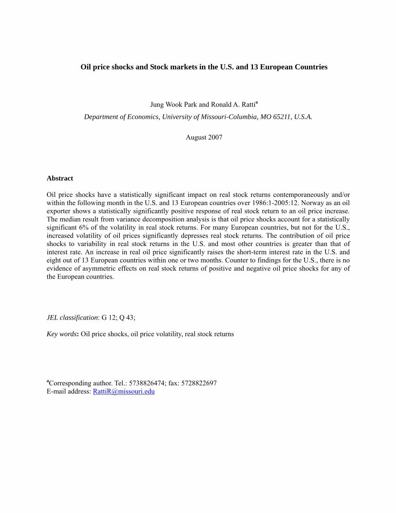
Index for all commodities and is shown in Figure 1. The world real oil price reflects a change in relative

price of oil faced by firms. In the latter half of the sample the pattern of oil price behavior is interesting in

4

that oil price increases are more frequent than oil price decreases. As an alternative to World real oil price

on which to base measurement of oil price shocks, a national real oil price is obtained for each country

using the exchange rate of and CPI of each country to adjust the nominal (dollar) price of oil.

In order to keep notation as simple as possible country suffices will be suppressed. The following

notation will be employed:

r: first log difference of short-term interest rate

ip: first log difference of industrial production

rsr: real stock returns

op : first log difference of real oil price (world or national)

2.2. Time series properties

The outcome of PP (Phillips and Perron (1988)) and KPSS (Kwiatkowski et al. (1992)) unit root

tests of the log levels and first log differences of real oil price, the short-term interest rate, and industrial

production, and of real stock returns are presented in Tables 2 and 3. In Tables 2 and 3 the null hypothesis

that real stock returns has a unit root is rejected at 5% level for the PP and KPSS tests.

In Table 2 for the PP test for the interest rate, real oil price, and industrial production, the null

hypotheses that the log level of each variable, has a unit root is not rejected at 5% level, and the null

hypotheses that the first log difference of each variable has a unit root is rejected at 5% level. In Table 3,

the KPSS test results with lag-truncation parameters of one and four, indicate that the null hypothesis that

variables in log level are level and trend stationary is rejected at the 5% level, and the null hypothesis that

variables in first log difference are level and trend stationary is not rejected at the 5% level. Thus, we

accept that in log levels, the interest rate, real oil price, and industrial production are I(1) processes, and

that real stock returns (rsr) and in first log differences, the interest rate, real oil price, and industrial

production are I(0) processes.

Since the variables the interest rate, oil price, and industrial production in log level each contain a

unit root, we conduct cointegration test (Johansen and Juselius (1990)) for common stochastic trend. The

results reported in Table 4 show that null hypothesis of no cointegration is rejected only for the U.K. (at

5

5% level of significance with world oil price and at 1% level of significance with national oil price), for

Italy (at 5% level of significance with world oil price), and for Finland (at 5% level of significance with

national oil price). In Table 4 the null hypothesis of no cointegration is not rejected in 24 out of 28 cases.

Given this outcome and the findings by Engle and Yoo (1987), Clements and Hendry (1995), and

Hoffman and Rasche (1996) that unrestricted VAR is superior in terms of forecast variance to a restricted

VECM at short horizons when the restriction is true, and by Naka and Tufte (1997) that the performance

of unrestricted VARs and VECMs for impulse response analysis over short-run is nearly identical, we will

run unrestricted VARs for all countries in what follows.

3. Oil price variables and Model

3.1. Non-Linear Oil price variables

Two transformations of oil price data that have been widely used in the literature will be utilized

in addition to first log difference of real oil price, op. These are scaled real oil price change due to Lee et

al. (1995), SOP, and the net oil price increase due to Hamilton (1996), NOPI. Lee et al. (1995) argue that

oil price shocks are more likely to have a significant impact in an environment in which oil prices have

been stable than in an environment where oil price movements have been frequent and erratic.

For the Lee et al. (1995) oil price specification, a GARCH(1,1) model is estimated for world real

oil price and for national real oil price for each country. This model is given by (country and world

suffices suppressed)

top = t

q

iiti

p

iiti zop εβαα +++ ∑∑

=−

=−

00

, ),0(~| 1 ttt hNI −ε , (1)

122

120 −− ++= ttt hh γεγγ ,

where top is first log difference in real oil price, log tε is an error term, and }1:{ 1 ≥− izt denotes an

appropriately chosen vector contained in information set 1−tI . The lags p and q are selected optimally for

world real oil price and national real oil price for each country. Scaled oil price is defined as (world and

6

country suffices are suppressed):

tSOP = tt h/ε , (2)

Net oil price increase, introduced by Hamilton (1996), is designed to capture how unsettling an

increase in the price of oil is likely to be for the spending decisions of consumers and firms. If the current

price of oil is higher than it has been in the recent past, then a positive oil price shock has occurred. Net

oil price increase is defined as:

tNOPI = max (0, tPlog – max ( 1log −tP ………. 6log −tP )), (3)

where tPlog is the log of level of real oil price at time t (world and country suffices are suppressed).

3.2. VAR Model

Our basic model is an unrestricted VAR with the four variables, first log difference of short-term

interest rate (r), real oil price (op), first log difference of industrial production (ip), and real stock returns

(rsr): VAR(r, op, ip, rsr). Here, country suffices are suppressed, and the oil price variable in different

VAR systems will be either first log difference of world real or national real oil prices or non-linear

transformations of real oil price changes defined as either scaled (SOP) or net (NOPI) real oil price

variables (in equations (2) and (3)). The ordering of the variables in the basic VAR implies that monetary

policy shocks are independent of contemporaneous disturbances to the other variables. This is the

ordering in Sadorsky (1999). VAR systems with different ordering and additional variables including oil

price volatility and inflation will also be estimated. The VAR(r, op, ip, rsr) is given by

∑ = − ++=k

i iitiOt uZAAZ1

(4)

where =tZ (r, op, ip, rsr)’, iA is a 4×4 matrix of unknown coefficients, oA is a column vector of

constant terms, tu is a column vector of errors with properties 0)( =tuE , all t, Ω=)( 'ttuuE , s=t, and

0)( ' =ttuuE , s ≠ t. k will be taken to be 6 for all VAR over the full sample.3

3 A check of optimal lag length based on LR, AIC, and BSIC criteria for the various VAR specifications across country and oil price variables yielded a range of results, with some less that 6 and some more than 6.

7

4. Impact of oil price shock on stock market

4.1.1. World real oil price shock

In this section we assess the impact of world real oil price shock on real stock returns by

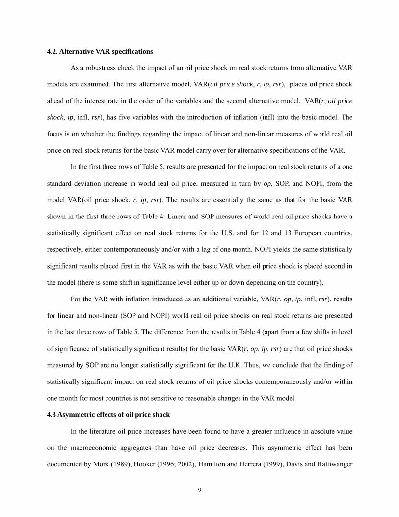
examining impulse response functions. The impulse responses of real stock returns from a one standard

deviation shock to oil price measured by the log first difference in real world oil price from the VAR(r, op,

ip, rsr) are shown in Figure 3. Results for 14 countries and 95% confidence bounds around each impulse

response appear in Figure 3.

For the U.S. and for ten of thirteen European countries (the exceptions are Norway, Finland, and

the U.K.) an oil price shock has a negative and statistically significant impact on real stock returns at the

5% level in the same month and/or within one month. In later months the impulse responses vary between

being negative and positive, with some statistically significant effects in some months for some countries.

Given that the effect being observed is for variable that is a (real) rate of return the impulse responses

revert to zero (usually well within 12 months). A transitory effect on the real rate of return on stocks is

expected. For Norway, an oil exporting country, oil price shock has a positive and statistically significant

impact on real stock returns at the 5% level in the same month and a positive but statistically insignificant

effect with a lag of one month.4 For Finland, a negative and statistically significant impact on real stock

returns with a lag of one month is obtained at the 10% level.

The first row of Table 4 summarizes the results in Figure 3. In Table 4 an n (p) indicates negative

(positive) statistically significant impulse response at 5% level of real stock return to oil price shock

contemporaneously and/or at lag of one month. The superscript # indicates that statistical significance is at

10% level. A summary of impulse response results for the impacts on real stock returns of shocks to the

non-linear transformations of world real oil price, SOP and NOPI, from the models VAR(r, SOP, ip, rsr)

and VAR(r, NOPI, ip, rsr), appear on lines 2 and 3 of Table 4. To economize on space, figures showing

the impulse responses are not reported, but for the oil price shock measure SOP they are similar to those

4 Oil prices increases are beneficial to Norwegian firms given the dependence of the economy on oil exports. Gjerde and Saettem (1999) also report a positive association between oil prices and Norwegian listed firm stock price and note that in the 1990s Norway exports were over 40% of GDP and dominated by exports of oil and natural gas.

8

in Figure 3 for the oil price shock measure op.

The second row of Table 4 shows that a one standard deviation increase in scaled world real oil

price (SOP) significantly impacts real stock returns in all countries contemporaneously and/or with a one

month lag. The results are negative with the exception of Norway, for which an oil price shock (SOP)

significantly raises real stock returns contemporaneously or within one month. Now, in contrast to the

result for a shock to op, a positive shock to scaled world real oil price reduces U.K. real stock returns

contemporaneously or within one month at the 10% level.5

In the third row of Table 4 results for the impact of net world real oil price (NOPI) on real stock

return are summarized. Net world real oil price has a statistically significant impact on real stock returns

for the U.S. and for 7 out of 13 of the European countries. The smaller number of statistically significant

results with NOPI compared to linear or scaled world real oil price shocks may be due to the pattern of oil

price increases and decreases in the period of study.

4.1.2. National real oil price shock

In rows four through six of Table 4 results are reported on the statistical significance of linear and

non-linear measures of national real oil price shocks on real stock returns. Linear and SOP measures of

national real oil price shocks have a statistically significant effect on real stock returns for the U.S. and for

10 and 9 European countries, respectively. NOPI national real oil price does not have a statistically

significant impact on real stock returns in as many countries as does linear or scaled national real oil price.

Generally, linear and non-linear measures of real oil price shocks measured as real world oil price yield

more cases of statistically significant impacts on real stock returns than do real oil price shocks measured

as national real oil price. For this reason, in what follows we will confine our attention to the impacts of

linear and non-linear measures of world real oil price.

5An outcome for the U.K. intermediate between that for Norway and the other European countries is not surprising. The U.K. is a net oil exporter over 1980 to 2004 since oil production minus domestic consumption is positive over this period, but negative starting in 2005 (http://europe.theoildrum.com/story/2006/9/17/135527/399). The value of net oil exports never achieved the relative importance for the U.K. economy as that achieved in the Norwegian economy. Jimenez-Rodriguez and Sanchez (2005) also report a difference between results for the U.K. and Norway, in that a positive oil price shock significantly reduces output in the U.K. and increases output in Norway.

9

4.2. Alternative VAR specifications

As a robustness check the impact of an oil price shock on real stock returns from alternative VAR

models are examined. The first alternative model, VAR(oil price shock, r, ip, rsr), places oil price shock

ahead of the interest rate in the order of the variables and the second alternative model, VAR(r, oil price

shock, ip, infl, rsr), has five variables with the introduction of inflation (infl) into the basic model. The

focus is on whether the findings regarding the impact of linear and non-linear measures of world real oil

price on real stock returns for the basic VAR model carry over for alternative specifications of the VAR.

In the first three rows of Table 5, results are presented for the impact on real stock returns of a one

standard deviation increase in world real oil price, measured in turn by op, SOP, and NOPI, from the

model VAR(oil price shock, r, ip, rsr). The results are essentially the same as that for the basic VAR

shown in the first three rows of Table 4. Linear and SOP measures of world real oil price shocks have a

statistically significant effect on real stock returns for the U.S. and for 12 and 13 European countries,

respectively, either contemporaneously and/or with a lag of one month. NOPI yields the same statistically

significant results placed first in the VAR as with the basic VAR when oil price shock is placed second in

the model (there is some shift in significance level either up or down depending on the country).

For the VAR with inflation introduced as an additional variable, VAR(r, op, ip, infl, rsr), results

for linear and non-linear (SOP and NOPI) world real oil price shocks on real stock returns are presented

in the last three rows of Table 5. The difference from the results in Table 4 (apart from a few shifts in level

of significance of statistically significant results) for the basic VAR(r, op, ip, rsr) are that oil price shocks

measured by SOP are no longer statistically significant for the U.K. Thus, we conclude that the finding of

statistically significant impact on real stock returns of oil price shocks contemporaneously and/or within

one month for most countries is not sensitive to reasonable changes in the VAR model.

4.3 Asymmetric effects of oil price shock

In the literature oil price increases have been found to have a greater influence in absolute value

on the macroeconomic aggregates than have oil price decreases. This asymmetric effect has been

documented by Mork (1989), Hooker (1996; 2002), Hamilton and Herrera (1999), Davis and Haltiwanger

10

(2001), and Balke et al. (2002), amongst others for the U.S., by Lee et al. (2001) for Japan, by Huang et

al. (2005) for Canada, Japan, and the U.S., and by Cunado and Perez de Garcia (2003) for most European

countries. An asymmetric effect is reported as a basic finding by Jones (2004) in their survey of the

literature on oil and the macreconomy.6 However, counter to this evidence Kilian (2007) reports that for

component expenditures of consumption and investment there is little evidence suggesting asymmetric

responses to positive and negative oil price shocks.

The issue of asymmetric effect of positive and negative oil price shocks on real stock returns will

be briefly examined here. In order to check for asymmetric effects of real oil price change, the first log

difference in world real oil price, top , will be separated into positive and negative real oil price changes

as in Mork (1989). The positive and negative real oil price changes in linear and scaled oil price shocks

are defined as:

topp = max (0, top ) and topn = min (0, top ) (5)

tSOPP = max (0, tSOP ), and tSOPN = min (0, tSOP ). (6)

In equations (5) and (6) op is first log difference in world real oil price and SOP is world scaled

oil price defined in equation (2). A 5 variable VAR will be estimated for each measure of oil price shock

by splitting oil price changes into oil price increases and oil price decreases: i.e. VAR(r, topp , topn , ip,

rsr) and VAR(r, tSOPP , tSOPN , ip, rsr) will be estimated. The test for asymmetry is a conventional Chi-

square ( 2χ ) test of the null hypothesis that the coefficients of positive and negative oil price shocks in the

VAR are equal to each other at each lag. For the sake of brevity results are summarized and not formally

presented here

The results obtained by carrying out this test of pair-wise of equality of the coefficients on

positive and negative oil price shocks are the following: the null hypothesis of symmetry cannot be

6 A number of explanations for asymmetric effects of oil price increases and decreases on aggregate activity have been advanced in literature, including adjustment costs and financial stress, but a consensus explanation does not seem to have emerged.

11

rejected for the European countries for linear and scaled oil price shocks, and cannot be rejected for the

U.S. for linear oil price shocks; for the U.S. the null hypothesis is rejected (at the 5% level of confidence)

for asymmetric effects on real stock returns of positive and negative scaled oil price shocks.7 Thus, we

conclude that there is no evidence for asymmetric effects of oil price shocks on European stock returns.

5. Oil Price Volatility

5.1. Definition of volatility

Increased volatility in energy prices can affect the present value of the discounted stream of

dividend payments, through increasing uncertainty about product demand and by increasing uncertainty

about the future return on investment. Bernanke (1983) and Pindyck (1991) argue that a firm faced with

increased uncertainty may delay implementing investment in capital equipment. We will construct an

indicator of uncertainty on the basis of daily data on oil prices. Measurement of monthly oil price

volatility (following Merton 1980 and Andersen et al. 2003) will be given by the sum of squared first log

differences in daily spot crude oil price:

∑=

+=ts

dtdtdtt sPPLogVol

1

2,1, )/)/(( , (7)

where dtP , is the spot price crude oil on day d of month t (obtained from NYMEX), and ts is the number

of trading days in month t. An alternative measure of oil price volatility could be given by the sum of

squared first log differences in daily futures (1 month) crude oil price

∑=

+=ts

dtdtdtt sFFLogVolf

1

2,1, )/)/(( , (8)

where dtF , is the futures crude oil price in day d of month t (obtained from NYMEX). However, since the

7 Although the null hypothesis of symmetric effects of oil price shocks on real stock returns is not rejected for the European countries for the full sample, the null hypothesis is rejected in a few cases for sub-samples. The question of sub-samples is of some interest in that the pattern of oil price fluctuation changed in the mid 1990’s, in that after this point oil price increases are more frequent than the oil price decreases and the magnitude of oil price increases is smaller than that of oil price decreases. For example, the null hypothesis of symmetry in effects of positive and negative oil price shocks on real stock returns is rejected for Spain and Germany over 1996:6-2005:12.

12

correlation of tVol and tVolf is 0.9586 and both measures yield very similar results we will present work

using tVol only.

tVol is represented in Figure 2. tVol is elevated at the time of the First Gulf War. The sharpest

spike is in January 1991. On January 12, 1991 the Congress of the U.S. authorized military force to

liberate Kuwait, on January 16, 1991 air strikes began against Iraq, and on January 17, 1991, Iraq fired

scud missiles against Israel.8 Volatility in oil price apparent over several months in 1986 may be due to

the switch by Saudi Arabia in early 1986 from selling its oil at official prices to a market-based pricing

system and thus changed from being a swing producer (with fluctuation in market share). As a result of

this shift, Saudi Arabia recaptured market share from the rest of OPEC and spot prices fell from $28 per

barrel in 1985 to $14 per barrel in 1986. The high level of volatility in oil price in March 2003 shown in

Figure 2 is presumably associated with the ongoing Iraqi disarmament crisis in early 2003 and the

invasion of Iraq on March 20, 2003 by U.S. and other forces.9

5.2. Effect of oil price volatility

Several VAR models will be estimated with tVol included as a variable. In the first model

volatility of oil price replaced oil price shock in the basic VAR model. Impulse response results of the

response of real stock returns to a one standard deviation shock to tVol in the model VAR(r, Vol, ip, rsr)

appears on the first line in Table 6. Oil price volatility has a significantly negative impact on the real stock

returns in 9 out of 14 countries. In particular, for the U.K., where impact of oil price shocks except for the

scaled oil price shock variable on real stock returns is not significant, volatility of oil prices depressed the

stock market. Volatility does not significantly affect real stock returns for the U.S..

Volatility is now included in the basic model along with oil price shocks. Impulse response results

of the response of real stock returns to a one standard deviation shock to tVol in the model VAR(r, op, Vol, 8 Iraq invaded Kuwait on August 2, 1990 (August 1990 is a spike in data on oil price volatility). A spike in oil price volatility in October 1990 might be associated, against the back drop of the Iraqi occupation of Kuwait, with an escalation in the Israeli-Palestinian conflict involving the Temple Mount in Jerusalem on October 8, 1990, and Syrian occupation of Mount Lebanon and ousting of the Lebanese government on October 13, 1990. 9 Huntington (2005) has an interesting discussion of historic oil supply disruptions. The measure of volatility in this paper might be a proxy variable for market expectations of future supply disruptions.

13

ip, rsr), where op is linear oil price shock (real oil price shock in first difference), appears on the second

line in Table 6 Impulse response results of the response of real stock returns to a one standard deviation

shock to linear oil price shock in the same five variable model appears on line 3 of Table 6. The result for

impact of linear oil price is essentially the same in this model as that found for the basic VAR(r, op, ip,

rsr) and reported on line 1 in Table 4 with statistically significant impulse responses contemporaneously

and/or with lag of one month for all countries except the U.K. Now however, real stock returns in the U.K

respond significantly and negatively to tVol even with op in the model. For the other countries, inclusion

of both op and tVol in the model only results in a significant and negative response to tVol in six cases.

The accumulated results of this section are that the effects of a shock to real world oil price on

real stock returns are robust to the inclusion of a measure of oil price uncertainty in the model. Oil price

shock is negatively related to real stock returns either contemporaneously or with a lag of one month. An

increase in the volatility of oil prices is also negative related to real stock returns either

contemporaneously or with a lag of one month in just over half the countries considered.

6. Oil price and interest rate shocks

6.1. Variance decomposition

Table 7 presents the forecast cast error variance decomposition of real stock returns due to the

interest rate and oil price shocks. Each percentage shows how much of the unanticipated changes of real

stock returns are explained by the variable indicated over a 24 month horizon. Results are presented based

on four models for world real oil price; linear and scaled (SOP) oil price shock specifications and the

basic VAR(r, oil price shock, ip, rsr) and alternative VAR(oil price shock, r, ip, rsr)).

The contribution of oil price shock to the real stock returns over a 24 month horizon ranges from

3.0% for the U.K. to 10.3% for Sweden in case of linear oil price shock and basic VAR specification in

column 2 of Table 7, with results being statistically significant in 12 out of 14 cases. The median result is

that oil price shocks account for about 6% of the volatility in real stock returns. Results for the

14

contribution of oil price shocks to variability in real stock returns are similar across the four models

reported in columns 2, 4, 6, and 8 of Table 7.10 Thus, variance decomposition suggests that oil price

shocks are a significant source of monthly volatility in real stock returns and are a prime factor when

considering real stock returns.11

The interest rate employed in the analysis is a short-term inter-bank rate that can be interpreted as

change in monetary policy. We find that the contribution of oil price shocks to variability in real stock

returns in the U.S. is greater than that of interest rate in all models. This result is consistent with the

finding by Sadorsky (1999) for the U.S. after 1986 that the contribution of oil price shock is greater than

that of interest rates on real stock returns. It is also consistent with finding by Davis and Haltiwanger

(2001) that oil price shocks account for about twice the variation in plant level employment as interest

rates.

These findings for the U.S. that oil price shocks have greater impact shocks to the interest are

similar are also found for Austria, Belgium, Finland, France, Germany, Greece, and Netherlands.

However, the interest rate contributes more to variability in real stock returns than oil price shocks for

Denmark, Italy, Norway, and Sweden. For Spain the contribution of the interest rate and oil price shocks

to variability in real stock returns are statistically significant and of about the same magnitude. Thus, for

somewhat less than half the European countries considered the relative magnitude of oil price shocks and

interest rate shocks as contributors to variability in real stock returns is different from that found for the

U.S. and serves to reinforce the need to examine behavior in many countries.

10 In results not reported models with variance compositions of real stock returns to oil price shocks at horizons of 6 and 12 months are very similar to those for the 24 month horizon in Table 8. Also not reported, we find that models with linear and SOP oil price specification show a bigger contribution of oil price shock to the real stock returns than models with NOPI oil price specification. 11 In some cases it is possible to make a comparison with results obtained by other researchers. For example, for Norway, Gjerde and Saettem (1999) report 24 month horizon variance decomposition for real stock returns of 6.2% and 5.0% from oil price and interest rate shocks over 1974 to 1994, quite similar to results in Table 7 for 1986 to 2005. Papapetrou (2001) in a study for Greece over 1989:1 to 1999:6 report 24 month horizon variance decomposition for real stock returns of 12.5% and 5.2% from shocks to consumer price index for fuels deflated by the consumer price index and the interest rate, respectively, that are larger than effects for related variables in Table 7. The relatively small number of observations in the latter study may be part of the explanation for the difference in results.

15

6.2 Impact of oil price shocks on interest rate

A number of papers investigate the connection between monetary policy and oil price shocks.

Bernanke et al. (1997) attribute the perceived association of oil price shocks and real growth to monetary

authority behavior, a view recently qualified by Hamilton and Herrera (2004). A rise in the interest rate

following oil price increases is interpreted as monetary policy tightening in anticipation of inflation

caused by oil price shock. The impact of oil price shock on the interest rate in the basic VAR is reported in

Table 8. Given the order of the VAR (r, oil price shock, ip, rsr) a one standard deviation oil price shock

can only affect the interest rate with a lag. In Table 8 a positive (negative) statistically significant impulse

response at 5% level of interest rate to oil price shock at a lag of one and/or two months is indicated by

the letter p (n). The superscript # indicates that statistic significance is at 10% level. The first row of Table

8 indicates that a one standard deviation increase in the world real oil price significantly raises the short-

term interest rate in the U.S. and eight out of 13 European countries with a lag of one or two months.12

The second row of Table 8 indicates that an increase in scaled oil price significantly raises the

short-term interest rate in seven and lowers the interest rate in two of the European countries with a lag of

one or two months. The negative response of the interest rate to SOP in two cases could be due to the fact

that SOP captures not just oil price change but also uncertainty about oil prices. The last row of Table 8

indicates that an increase in net oil price significantly raises the short-term interest rate in the U.S. and in

eight European countries.

7. Conclusion

The vast literature establishing robust results across many countries on the connection between

oil price shocks and aggregate activity implies that connections should also hold between oil price shocks

and stock markets. This study estimates the effects of oil price shocks and oil price volatility on the real

12 A review of the literature on monetary policy and oil price shocks is provided by Cologni and Manera (2007). The finding of no significant connection between interest rates and oil prices has been reported for some countries and sample periods. Cologni and Manera (2007) report, on the basis of quarterly data over 1980Q1-2003Q3, that among the G-7 there is a monetary policy reaction of rising interest rates in response to higher oil prices for the U.S., but a tendency to the reverse for Canada, France and Italy. In this analysis stock price play no role.

16

stock returns of the U.S. and 13 European countries over 1986:1-2005:12 using a multivariate VAR

analysis. We find that oil price shocks have a statistically significant impact on real stock returns in the

same month or within one month and that this result is robust to reasonable changes in the VAR model of

variable order and inclusion of additional variables. Linear and scaled measures of real oil price shocks

calculated as world real oil price rather than national real oil price yield most cases of statistically

significant impacts on real stock returns. The median result from variance decomposition analysis is that

oil price shocks account for a statistically significant 6% of the volatility in real stock returns.

Other results for the effect of oil price shocks on stock prices vary between countries, with the

U.S. pattern varying between being an outlier and representing the majority outcome depending on issue

addressed. For many European countries, but not for the U.S., increase in the volatility of oil prices

significantly depresses real stock returns contemporaneously or within one month. For the U.S. and about

half the European countries the contribution of oil price shocks to variability in real stock returns is

greater than that of the interest rate. A one standard deviation increase in the world real oil price

significantly raises the short-term interest rate in the U.S. and eight out of 13 European countries at a lag

of one or two months. Finally, while there is some evidence of asymmetric effects on real stock returns of

positive and negative oil price shocks for the U.S. there is none for any of the European countries.

Additional research should be directed to investigating the mechanisms by which oil price and energy

prices affect firm behavior and stock price.

17

Appendix- Data Sources

Monthly data over 1986.1 to 2005.12.

Countries: Austria, Belgium, Denmark, Finland, France, Germany, Greece, Italy, Netherlands, Norway, Spain,

Sweden, U.K., U.S.

Nominal oil price: IMF data from IFS. U.K. Brent (11276AADZF)

Real oil price of World: Nominal oil price deflated by the U.S. PPI

Real oil price of each country: Product of nominal oil price and exchange rate (#/U.S. $)deflated by the CPI of each

country

U.S.

Consumer Price Index: FRED (Federal Reserve Economic Data). Consumer Price Index for All Urban Consumers

All Items (CPIAUCSL), seasonally adjusted.

Industrial Production: FRED. Industrial Production Index (INDPRO, 2002 = 100), seasonally adjusted.

Share Prices: S&P 500 Index From COMPUSTAT NORTH AMERICA (I0002-S&P 500 comp-Ltd).

Short-term interest rate: FRED. 3 month Treasury-bill (TB3MS).

Producer Prices Index: FRED. Producer Price Indexes All commodities (PPIACO)

European countries

Exchange Rate: FRED. Number of units of currency per U.S. dollar.

Consumer Price Index: OECD. Data from Main Economic Indicators (2000 = 100), seasonally adjusted with X-11

procedure.

Industrial Production: OECD. Data from Main Economic Indicator (seasonally adjusted).

Share Price: OECD. Data from Main Economic Indicators, except for Finland from IMF (17262...ZF. industrial).

Short-term interest rate: IMF data from IFS for Germany, Belgium, Spain, Greece, Sweden, U.K. (Treasury bill rate

- line 60c), for Finland, Italy, Denmark, Norway (Money market rate – line 60 b). For Austria data are from OECD

data from Main Economic Indicators. For Netherlands, data are call money rate from Bank of Netherlands. For

France, data are money market rate from INSEE (National Institute for Statistics and Economic Studies).

18

References Andersen, T. G.., Bollerslev, T., Diebold, F. X., Labys, P., 2003. Modeling and Forecasting Realized Volatility. Econometrica 71 (2), 579-625. Balaz, P., Londarev, A., 2006. Oil and its position in the process of globalization of the world economy. Politicka Ekonomie 54 (4), 508-528. Balke, N. S., Brown, S. P. A., Yucel, M. K., 2002. “Oil price shocks and the U.S. Economy: where does the asymmetry originate ?” Energy Journal 23(3), 27-52. Barsky, R.B., Kilian L., 2004. “Oil and the Macroeconomy since the 1970s.” Journal of Economic Perspectives 18, 115-134. Bernanke, B. S., 1983. “Irreversibility, Uncertainty, and Cyclical Investment.” Quarterly Journal of Economics 98, 85-106. Bernanke, B. S., Gertler, M., Watson, M., 1997. “Systemic monetary policy and the effects of oil price shocks.” Brookings papers on economic activity 1, 91-157. Ciner, C., 2001. “Energy shocks and financial markets: Nonlinear linkages.” Studies in Non-Linear Dynamics and Econometrics 5, 203-212. Clements, M. P., Hendry, D. F., 1995. “Forecasting in Cointegrated System.” Journal of Applied Econometrics 10, 127-146. Cologni, A., Manera, M., 2007. “Oil prices, inflation and interest rates in a structural cointegrated VAR model for the G-7 countries.” Forthcoming in Energy Economics. Cunado, J., Perez de Garcia, F., 2003. “Do oil price shocks matter? Evidence for some European countries.” Energy Economics 25, 137-154 Cunado, J., Perez de Garcia, F., 2005. “Oil prices, economic activity and inflation: evidence for some Asian countries.” The Quarterly Review of Economics and Finance 45 (1), 65-83. Davis, S. J., Haltiwanger, J., 2001. “Sectoral job creation and destruction response to oil price changes.” Journal of Monetary Economics 48, 465-512. Engle, R. F., Yoo, B. S., 1987. “Forecasting and Testing in cointegrated system.” Journal of Econometrics 35, 143-159. Gjerde, O., Saettem, F., 1999. “Causal relations among stock returns and macroeconomic variables in a small, open economy.” Journal of International financial market, Institutions and Money 9, 61-74. Hamilton, J. D., 1983. “Oil and the Macroeconomy since World War II.” Journal of Political Economy 91:228-248. Hamilton, J. D., 1996. “This is what happened to the Oil price-Macroeconomy Relationship.” Journal of Monetary Economics 38, 215-220. Hamilton, J. D., 2005. “Oil and the Macroeconomy.” Forthcoming in Durlauf, S., Blume, L. (Eds), The

19

New Palgrave Dictionary of Economics, 2nd ed., Palgrave MacMillan Ltd. Hamilton, J. D., Herrera, A. M., 2004. “Oil shocks and aggregate macroeconomic behavior: the role of monetary policy.” Journal of Money, Credit, and Banking 36(2), 265-286. Hoffman, D. L., Rasche, R. H., 1996. “Assessing Forecast performance in a Cointegrated system.” Journal of Applied Econometrics 11, 495-517. Hooker, M. A., 1996. “What happened to the Oil price-Macroeconomy Relationship.” Journal of Monetary Economics 38, 195-213. Hooker, M. A., 2002. “Are Oil Shocks Inflationary? Asymmetric and Nonlinear Specifications versus Changes in Regime.” Journal of Money, Credit and Banking 34, 540-561. Huang, B.-N., Hwang, M. J., Peng, H.-P., 2005. “The asymmetry of the impact of oil price shocks on economic activities: An application of the multivariate threshold model.” Energy Economics 27, 445-476 Huang, R. D., Masulis, R. W., Stoll, H. R., 1996. “Energy shocks and financial markets.” Journal of Futures Markets 16, 1-27. Huntington, H. G., 2005. “The economic consequences of higher crude oil prices.” Energy Modeling Forum. Final Report EMF SR9. Stanford University. Jimenez-Rodriguez, R., Sanchez, M., 2005. “Oil price shocks and real GDP growth: empirical evidence for some OECD countries.” Applied Economics 37 (2), 201-228. Johansen, S., Juselius, K., 1990. “Maximum likelihood estimation and inference on Cointegration -with applications to demand for money.” Oxford Bulletin of Economics and Statistics 52, 169-210. Jones, C. M., Kaul, G., 1996. “Oil and the Stock Market.” Journal of Finance 51, 463-491. Jones, D. W., Leiby, P. N., Paik, I. K., 2004. “Oil price shocks and the Macroeconomy: what has been learned since 1996.” The Energy Journal 25, 1-32. Kilian, L., 2007. “The Economic Effects of Energy Price Shocks.” Forthcoming in Journal of Economic Literature. Kwiatkowski, D., Phillips, P. C. B., Schmidt, P., Shin, Y., 1992. “Testing the null hypothesis of stationarity against the alternative of a unit root.” Journal of Econometrics 54, 159-178. Lee, B. R., Lee, K., Ratti, R. A., 2001. “Monetary Policy, Oil Price Shocks, and Japanese Economy.” Japan and the World Economy 13, 321-349. Lee, C.-C., Chang, C.-P., 2007. “Energy consumption and GDP revisited : A panel analysis of developed and developing countries.” Forthcoming in Energy Economics. Lee, K., Ni, S., Ratti. R. A., 1995. “Oil shocks and the Macroeconomy: The role of Price Variability.” Energy Journal 16(4), 39-56. Merton, R. C., 1980. “On Estimating the Expected Return on the Market: An Explanatory Investigation,” Journal of Financial Economics.” 8(4), 323-61.

20

Mork, K. A., 1989. “Oil and the Macroeconomy when Prices Go Up and Down: An Extension of Hamilton’s Results.” Journal of Political Economy 97, 740-744 Naka, A., Tufte, D., 1997. “Examining Impluse Response Functions in Cointegrated system.” Applied Economics 29, 1593-1603. Papapetrou, E., 2001. “Oil price Shocks, Stock Market, Economic Activity and Employment In Greece.” Energy Economics 23, 511-532. Phillips, P.C.B., Perron, P., 1988. “Testing for a unit root in time series regression.” Biometrika 75, 335-346. Pindyck, R., 1991. “Irreversibility, uncertainty and investment.” Journal of Economic Literature. 29(3), 1110-1148. Sadorsky, P., 1999. “Oil Price Shocks and Stock Market Activity.” Energy Economics 21, 449-469. Sadorsky, P., 2006. “Modeling and Forecasting Petroleum Futures Volatility.” Energy Economics 28, 467-488.

21

Figure 1. World real oil price (Dollar index of U.K. Brent/PPI for all commodities)

Figure 2. Monthly oil price volatility (Normalized sum of squared first log difference in daily spot crude oil price)

0

50

100

150

World real oil price

1985 1990 1995 2000 2005

0

2

4

6

8

10

Volatility

1985 1990 1995 2000 2005

Figure 3. World real oil price shocks: Impulse response function of real stock returns to linear oil price shocks in VAR(r, op, ip, rsr)

-.01

0

.01

0 10 20 30

us, dlroil, rsr

95% CI orthogonalized irf

step

Graphs by irfname, impulse variable, and response variable

-.02

-.01

0

.01

0 10 20 30

austria, dlroil, rsr


step


-.02

-.01

0

.01

0 10 20 30

belgium, dlroil, rsr


step


-.01

-.005

0

.005

0 10 20 30

denmark, dlroil, rsr


step


-.02

-.01

0

.01

.02

0 10 20 30

finland, dlroil, rsr


step


-.02

-.01

0

.01

0 10 20 30

france, dlroil, rsr


step


-.02

-.01

0

.01

0 10 20 30

germany, dlroil, rsr


step


-.04

-.02

0

.02

0 10 20 30

greece, dlroil, rsr


step


-.02

-.01

0

.01

0 10 20 30

ital, dlroil, rsr


step


-.02

-.01

0

.01

0 10 20 30

netherlands, dlroil, rsr


step


-.02

-.01

0

.01

.02

0 10 20 30

norway, dlroil, rsr


step


-.02

-.01

0

.01

0 10 20 30

spain, dlroil, rsr


step


-.02

-.01

0

.01

.02

0 10 20 30

sweden, dlroil, rsr


step


-.01

-.005

0

.005

.01

0 10 20 30

uk, dlroil, rsr


step

Graphs by irfname, impulse variable, and response variable Notes : Figures are: first row - U.S., Austria, Belgium, Denmark; second row - Finland, France, Germany, Greece; third row - Italy, Netherlands, Norway, Spain; fourth row – Sweden, U.K. In VAR(r, op, ip, rsr), r, op, and ip, are the short-term interest rate, world real oil price, and industrial production in first log difference, and rsr is real stock return.

23

Table 1. PP Unit Root Test Results Real oil price Interest rates log level first log difference log level first log difference Country C C&T C C&T C C&T C C&T World -2.186 -2.995 -13.152a -13.155a U.S. -2.392 -2.711 -12.998a -13.012a -1.394 -1.273 -8.982a -9.000a Austria -2.183 -2.938 -12.921a -12.926a -0.279 -1.582 -11.073a -11.137a Belgium -2.189 -3.003 -13.102a -13.139a -0.879 -1.924 -11.135a -11.111a Denmark -2.646c -3.250c -13.062a -13.092a -0.730 -2.525 -12.483a -12.419a Finland -2.030 -3.528b -13.202a -13.230a -0.787 2.040 -10.372a -10.348a France -2.303 -3.078 -12.920a -12.927a -0.672 -2.087 -13.099a -13.074a Germany -2.093 -2.848 -12.920a -12.927a -0.920 -1.765 -14.078a -14.077a Greece -2.867b -3.011 -13.013a -13.051a 0.536 -1.957 -11.629a -11.716a Italy -2.559 -3.625b -12.992a -13.017a -0.597 -2.060 -11.125a -11.097a Netherlands -2.560 -3.145c -13.057a -13.083a -0.679 -1.791 -16.980a -16.970a Norway -2.422 -3.311c -13.347a -13.376a -1.326 -2.690 -16.528a -16.496a Spain -2.723c -3.507b -13.049a -13.084a -0.519 -2.527 -12.979a -12.986a Sweden -1.885 -3.194c -12.979a -13.020a -0.076 -2.026 -12.453a -12.467a U.K. -2.974b -3.171c -13.421a -13.453a -1.369 -1.968 -9.188a -9.181a

Industrial production Real stock returns log level first log difference (rsr) Country C C&T C C&T C C&T U.S. -0.439 -1.170 -14.286a -14.260a -15.427a -15.42a Austria -0.204 -2.893 -27.118a -27.218a -13.645a -13.674a Belgium -0.963 -4.755a -29.321a -29.253a -9.872a -9.840a Denmark -1.149 -6.383a -19.804a -19.760a -12.580a -12.605a Finland -0.093 -2.141 -23.928a -23.894a -10.631a -10.616a France -0.837 -2.086 -23.965a -23.936a -12.801a -12.775a Germany -0.634 -2.060 -22.957a -22.919a -14.537a -14.510a Greece -1.406 -3.959b -30.979a -30.956a -1.892a -10.906a Italy -2.206 -2.245 -18.951a -19.095a -12.118a -12.095a Netherlands -1.631 -9.042a -35.235a -35.144a -10.445a -10.423a Norway -1.929 -3.643b -31.645a -32.232a -13.038a -13.044a Spain -0.865 -2.522 -28.484a -28.427a -12.882a -12.849a Sweden -0.423 -2.311 -18.812a -18.769a -10.404a -1.383a U.K. -2.885b -1.735 -22.986a -23.852a -12.151a -12.137a

Notes: PP – Phillips and Perron (1988); C – constant; T – trend. World refers to the world real price of oil. Superscripts a, b, and c, denote rejection of the null hypothesis of a unit root at the 1%, 5%, and 10%, level of significance, respectively.

24

Table 2. KPSS Unit Root Test Results

Real oil price in log level Real oil price in first log difference lag = 1 lag = 4 lag = 1 lag = 4 Country L T L T L T L T World 3.16a 1.39a 1.37a 0.613a 0.132 0.0213 0.135 0.0220 U.S. 1.77a 1.45a 0.77a 0.632a 0.162 0.0242 0.162 0.0245 Austria 3.18a 1.39a 1.37a 0.605a 0.154 0.0249 0.151 0.0247 Belgium 3.36a 1.36a 1.44a 0.591a 0.151 0.0247 0.147 0.0244 Denmark 2.54a 1.56a 1.11a 0.683a 0.220 0.0271 0.217 0.0273 Finland 4.95a 1.33a 2.13a 0.591a 0.201 0.0269 0.202 0.0274 France 3.11a 1.61a 1.34a 0.702a 0.205 0.0256 0.205 0.0261 Germany 3.23a 1.44a 1.39a 0.623a 0.156 0.0252 0.153 0.0248 Greece 1.84a 1.74a 0.80a 0.756a 0.229 0.0260 0.230 0.0267 Italy 3.64a 1.34a 1.59a 0.597a 0.196 0.0269 0.197 0.0275 Netherlands 2.5a 1.50a 1.02a 0.658a 0.199 0.0268 0.197 0.0269 Norway 3.22a 1.44a 1.40a 0.636a 0.194 0.0245 0.203 0.0261 Spain 3.10a 1.56a 1.35a 0.689a 0.216 0.0266 0.217 0.0271 Sweden 4.67a 1.68a 2.00a 0.739a 0.226 0.0238 0.228 0.0244 U.K. 1.54a 1.39a 0.68b 0.615a 0.188 0.0234 0.193 0.0244 Interest rate in log level Interest rate in first log difference lag = 1 lag = 4 lag = 1 lag = 4 Country L T L T L T L T U.S. 5.99a 0.766a 2.42a 0.314a 0.270 0.247a 0.158 0.145c Austria 6.98a 1.180a 2.83a 0.483a 0.360c 0.140c 0.259 0.102 Belgium 9.89a 0.800a 4.02a 0.330a 0.088 0.087 0.071 0.070 Denmark 10.00a 0.732a 4.09a 0.310a 0.083 0.059 0.079 0.057 Finland 10.40a 0.741a 4.23a 0.308a 0.097 0.096 0.081 0.081 France 10.00a 0.853a 4.06a 0.354a 0.092 0.075 0.085 0.069 Germany 6.27a 1.360a 2.54a 0.556a 0.198 0.118 0.167 0.101 Greece 10.50a 2.680a 4.26a 1.090a 0.603 0.193b 0.045 0.148b Italy 10.80a 1.560a 4.37a 0.645a 0.101 0.084 0.075 0.063 Netherlands 7.85a 0.895a 3.19a 0.366a 0.168 0.119c 0.139 0.099 Norway 7.90 a 0.644a 3.23a 0.269a 0.056 0.056 0.048 0.048 Spain 10.50a 1.340a 4.26a 0.559a 0.186 0.113 0.135 0.083 Sweden 10.50a 1.060a 4.27a 0.443a 0.135 0.050 0.120 0.045 U.K. 9.02a 0.485a 3.67a 0.201b 0.106 0.090 0.074 0.063

Notes: KPSS – Kwiatkowski et al. (1992); L - level stationarity; T - trend stationarity. World refers to the world real price of oil. Superscripts a, b, and c, denote rejection of the null hypothesis at the 1%, 5%, and 10%, level of significance, respectively.

25

Table 2-continued. KPSS Unit Root Test Results Industrial production in log level Industrial production in first log difference lag = 1 lag = 4 lag = 1 lag = 4 Country L T L T L T L T U.S. 11.9a 1.21a 4.81a 0.491a 0.290 0.284a 0.190 0.186 b Austria 11.7a 1.55a 4.74a 0.652a 0.0508 0.025 0.0994 0.0493 Belgium 10.8a 1.04a 4.42a 0.459a 0.0219 0.0191 0.0392 0.0341 Denmark 11.5a 0.64a 4.75a 0.357a 0.0133 0.0096 0.0261 0.0187 Finland 11.6a 1.65a 4.69a 0.684a 0.0872 0.0651 0.1370 0.1020 France 10.9a 0.933a 4.42a 0.385a 0.064 0.0639 0.0801 0.0796 Germany 9.45a 0.78a 3.87a 0.323a 0.0070 0.0698 0.0881 0.0825 Greece 9.56a 1.84a 3.93a 0.795a 0.026 0.0193 0.0579 0.0431 Italy 10.1a 0.999a 4.11a 0.420a 0.204 0.046 0.2210 0.0512 Netherlands 11.6a 0.799a 4.75a 0.405a 0.0179 0.0072 0.0387 0.0157 Norway 10.6a 2.49a 4.35a 1.090a 0.0618 0.0076 0.165 0.0208 Spain 11.0a 1.05a 4.46a 0.436a 0.0492 0.0498 0.0726 0.0735 Sweden 11.9a 0.98a 4.81a 0.412a 0.0607 0.0608 0.0816 0.0818 U.K. 10.0a 1.33a 4.09a 0.557a 0.389c 0.0595 0.566b 0.0943

Real stock returns (rsr) lag = 1 lag = 4 Country L T L T U.S. 0.143 0.081 0.160 0.091 Austria 0.225 0.125c 0.187 0.105 Belgium 0.098 0.091 0.092 0.085 Denmark 0.128 0.071 0.103 0.058 Finland 0.112 0.099 0.098 0.087 France 0.082 0.068 0.071 0.059 Germany 0.078 0.075 0.072 0.069 Greece 0.199 0.093 0.166 0.079 Italy 0.096 0.082 0.081 0.071 Netherlands 0.164 0.156b 0.141 0.134c Norway 0.109 0.058 0.097 0.052 Spain 0.098 0.090 0.106 0.097 Sweden 0.091 0.086 0.075 0.071 U.K. 0.127 0.065 0.122 0.063

Notes: KPSS – Kwiatkowski et al. (1992); L - level stationarity; T - trend stationarity. Superscripts a, b, and c, denote rejection of the null hypothesis at the 1%, 5%, and 10%, level of significance, respectively.

26

Table 3. Cointegration test results for 14 countries (Variables: interest rate, real oil price, and industrial production in log levels)

World real oil price

Country Hypothesis r=0 r =< 1 r=<2 Country Hypothesis r=0 r =< 1 r=<2

U.S. Trace test 14.619 6.859 1.104 Greece Trace test 28.273 6.032 0.025

λ max test 7.760 5.754 1.104 λ max test 22.241b 6.007 0.025

Austria Trace test 27.783 5.557 0.243 Italy Trace test 30.902b 7.501 1.663


Belgium Trace test 24.673 6.225 0.243 Neth. Trace test 17.129 7.814 2.186

λ max test 18.449 5.982 0.243 λ max test 9.315 5.627 2.186

Denmark Trace test 16.362 5.054 0.04 Norway Trace test 26.353 7.527 1.683


Finland Trace test 27.601 8.682 0.404 Spain Trace test 24.064 6.730 0.806


France Trace test 27.922 5.930 0.246 Sweden Trace test 15.379 4.027 0.0004

λ max test 21.992b 5.684 0.246 λ max test 11.352 4.020 0.0004

Germany Trace test 16.477 6.850 0 U.K. Trace test 41.936b 4.330 1.891


National real oil price

Country Hypothesis r=0 r =< 1 r=<2 Country Hypothesis r=0 r =< 1 r=<2

U.S. Trace test 14.469 7.070 1.201 Greece Trace test 27.708 5.215 0.051

λ max test 7.399

5.869 1.201 λ max test 20.494 5.164 0.051

Austria Trace test 25.783 5.557 0.243 Italy Trace test 27.404 8.794 1.155


Belgium Trace test 28.609 9.670 0.467 Neth. Trace test 18.388 9.714 3.355


Denmark Trace test 17.747 5.503 0.1 Norway Trace test 24.520 8.517 2.152


Finland Trace test 29.819b 6.985 0.172 Spain Trace test 23.654 7.848 0.316

λ max test 22.839b 6.813 0.172 λ max test 15.806 7.532 0.316

France Trace test 28.714 7.984 0.486 Sweden Trace test 16.028 5.458 0.139


Germany Trace test 17.861 7.356 0.0001 U.K. Trace test 38.322a 5.778 2.189

λ max test 10.505 7.356 0.0001 λ max test 32.544a 3.589 2.189 Notes: Johansen and Juselius (1990) test statistic for cointegration. World real oil price - dollar index of U.K. Brent/PPI in log level, National real oil price - dollar index of U.K. Brent/[(dollar price national currency)(national CPI)] in log level. The number of cointegrating vectors is indicated by r. Superscripts a and b denote rejection of the null hypothesis at the 1% and 5% levels of significance, respectively.

27

Table 4. Statistically Significant Impulse Response of Real Stock Return to Real Oil Price Shock: VAR(r, oil price shock, ip, rsr). (Contemporaneously and/or with lag of one month)

Notes: n (p) indicates negative (positive) statistically significant impulse response at 5% level of real stock return to oil price shock contemporaneously and/or a lag of one month. The superscript # indicates that statistic significance is at 10% level. In VAR(r, oil price shock, ip, rsr), r and ip are the short-term interest rate and industrial production in first log difference and rsr is real stock return. Oil price shock is measured as first log difference in world real oil price or in national real oil price or as non-linear transformations of these variables. SOP denotes scaled oil price change and NOPI indicates net oil price change. World real oil price - (U.S. dollar index for U.K. Brent crude oil)/(U.S. PPI for all commodities). National real oil price for country i – [(U.S. dollar index for U.K. Brent crude oil)(units of currency country i per U.S. dollar)]/(CPI for country i).

U.S. AUS BEL DEN FIN FRA GER GRE ITA NET NOR SPA SWE U.K.

World real Oil price Sign of statistically significant effect on real stock returns of shock to World real oil price

Shock to op n n n n n# n n n n n p n n

Shock to SOP n n n n n# n n n n n p n n n#

Shock to NOPI n# n# n# n n n n# n#

National real

Oil price Sign of statistically significant effect on real stock returns of shock to National real oil price

Shock to op n n n n n n n n n# p n

Shock to SOP n n n n n n n n# p n

Shock to NOPI n n# n n n# n

28

Table 5. Statistically Significant Impulse Response of Real Stock Return to Real World Oil Price Shock: Alternative VARs (Contemporaneously and/or with lag of one month)

Notes: n (p) indicates negative (positive) statistically significant impulse response at 5% level of real stock return to oil price shock contemporaneously and/or a lag of one month. The superscript # indicates that statistic significance is at 10% level. infl, r, and ip are the consumer price index, short-term interest rate and industrial production in first log difference and rsr is real stock return. Oil price shock is measured as first log difference in world real oil price or as non-linear transformations of this variable. SOP denotes scaled oil price change and NOPI indicates net oil price change. World real oil price - (U.S. dollar index for U.K. Brent crude oil)/(U.S. PPI for all commodities).


Sign of statistically significant effect on real stock returns in VAR(oil price shock, r, ip, rsr)


Shock to SOP n n n n n# n n n n n p n n n#

Shock to NOPI n# n# n n n n# n# n

Sign of statistically significant effect on real stock returns in VAR(r, oil price shock, ip, infl, rsr).


Shock to SOP n n n n n n n n n n p n n

Shock to NOPI n n n n# n n n n n

29

Table 6. Statistically Significant Impulse Response of Real Stock Return to Oil Price Volatility and/or World Real Oil Price (Contemporaneously and/or with lag of one month)

Notes: n (p) indicates negative (positive) statistically significant impulse response at 5% level of real stock return to Vol and/or oil price shock contemporaneously and/or a lag of one month. The superscript # indicates that statistic significance is at 10% level. Vol is oil price volatility – normalized sum of squares of first log difference in daily spot oil price. Oil price shock, op, is measured as first log difference in world real oil price. r and ip are the short-term interest rate and industrial production in first log difference and rsr is real stock return. World real oil price - (U.S. dollar index for U.K. Brent crude oil)/(U.S. PPI for all commodities).


Sign of statistically significant effect on real stock returns in VAR(Vol, r, ip, rsr)

Shock to Volatility n n n n# n n n n n

Sign of statistically significant effect on real stock returns in VAR(r, op, Vol, ip, rsr)

Shock to Volatility n n# n n n n n


30

Table 7. Variance decomposition of variance in real stock returns due to world real oil price and interest rate shocks

Percentage of Variation in real stock returns due to shocks interest rate or oil price (24 month horizon)

VAR model: VAR(r, op, ip, rsr) VAR(r, SOP, ip, rsr) VAR(op, r, ip, rsr) VAR(SOP, r, ip, rsr)

Shock to: 1

Due to r 2

Due to op 3

Due to r 4

Due to SOP 5

Due to r 6

Due to op 7

Due to r 8

Due to SOP

U.S. 1.11 5.86b 1.17 4.41c 0.98 5.96b 1.14 4.44c

Austria 2.98 4.03c 2.93 3.31 2.95 4.06c 2.94 3.31

Belgium 2.33 8.50b 2.49 7.00c 2.01 8.79b 2.20 7.27c

Denmark 4.22c 2.92 4.28 c 2.82 4.42c 2.72 4.43c 2.67

Finland 2.87 5.61b 2.74 4.66b 2.99 5.49b 2.75 4.65c

France 1.08 5.86b 1.21 4.80c 1.05 5.89b 1.20 4.81c

Germany 3.02 7.54b 2.63 6.90b 3.03 7.53b 2.61 6.91b

Greece 2.34 8.34b 2.14 8.70b 2.44 8.24b 2.27 8.57b

Italy 13.72a 9.69a 14.06a 9.38a 13.61a 9.81a 13.88a 9.56a

Netherlands 1.45 7.34b 1.49 6.56b 1.26 7.53b 1.26 6.79b

Norway 8.92b 5.96b 9.27b 5.09c 8.95b 5.93b 9.33b 5.03c

Spain 4.84b 4.67c 4.18c 4.75c 4.84c 4.67c 4.18c 4.75c

Sweden 9.91b 10.28a 9.57b 8.84b 9.91b 10.28a 9.62b 8.79b

U.K. 3.86 3.01 4.36 2.95 4.06 2.81 4.52c 2.79 Notes: Oil price shock is measured as first log difference in world real oil price, op, or as non-linear transformation real world oil price, scaled oil price (SOP). r and ip are the short-term interest rate and industrial production in first log difference and rsr is real stock return. World real oil price - (U.S. dollar index for U.K. Brent crude oil)/(U.S. PPI for all commodities). Superscripts a, b, c, denote statistical significance at the 1%, 5%, 10% levels.

31

Table 8. Statistically Significant Impulse Response of Interest Rate to World Real Oil Price (Statistically significant effect of oil price shock at first and/or second lag)

Notes: n (p) indicates negative (positive) statistically significant impulse response at 5% level of real stock return to oil price shock at first and/or second lag. The superscript # indicates that statistic significance is at 10% level. Oil price shock is measured as first log difference in world real oil price, op, or as non-linear transformation real world oil price, scaled oil price (SOP) or net oil price change (NOPI). r and ip are the short-term interest rate and industrial production in first log difference and rsr is real stock return. World real oil price - (U.S. dollar index for U.K. Brent crude oil)/(U.S. PPI for all commodities).

Sign of statistically significant effect on interest rate of world oil price in VAR(r, oil price shock, ip, rsr)

World real Oil price U.S. AUS BEL DEN FIN FRA GER GRE ITA NET NOR SPA SWE U.K.

Shock to op p# p p p p p p p p

Shock to SOP p n p p p p n# p p

Shock to NOPI p# p p p p p p p p

Documents

Oil price shocks and Stock markets in the U.S. and 13 European