Oil Shocks and Stock Return Volatility ∗

Lance J. Bachmeier a Soheil R. Nadimi b

Department of Economics, Kansas State University

Abstract

Asset return volatility is important to the macroeconomy. This paper asks whetheroil price volatility can be used as a predictor of stock return volatility. In contrastwith previous research, we focus on the out-of-sample predictive power of oil pricevolatility rather than on in-sample inference. Formal tests of out-of-sample predictiveability find no evidence supporting the use of oil price volatility as a predictor offuture stock return volatility. Further analysis using rolling window estimationand structural break tests shows that the coefficients of this relationship are veryunstable. The coefficients can be positive, negative, or close to zero depending onthe sample that is chosen. We discuss the implications of this finding for monetarypolicy.

JEL classification: G17; Q41

Keywords: Oil price; Stock return; Volatility; Prediction

Declarations of interest: none

∗This research did not receive any specific grant from funding agencies in the public, commercial, ornot-for-profit sectors.

a327 Waters Hall, Department of Economics, Kansas State University, Manhattan, KS 66506, USA.Tel: +1 (785) 532-4578. E-mail: lanceb@ksu.edu.

bCorresponding Author. 327 Waters Hall, Department of Economics, Kansas State University,Manhattan, KS 66506, USA. Tel: +1 (785) 317-3032. E-mail: soheil@ksu.edu.

1

1 Introduction

The volatility of asset prices is believed by many to have important effects on the

macroeconomy (see e.g. Phelps, 1999). This suggests that monetary and fiscal policy

should be made taking into account the volatility of asset prices, and in particular, the

volatility of stock prices. Farmer (2012) has advocated a policy of direct government

intervention to reduce the volatility of the stock prices. If these views are correct, and

the government should be offsetting or even preventing volatility of stock prices, it is

important to find good predictors of stock price volatility. An obvious candidate is oil price

volatility. There are many published estimates of the effect of oil shocks on macroeconomic

variables.1 A growing literature has found evidence that oil price shocks have an effect on

stock prices,2 with most authors finding that higher oil prices have a negative effect on

stock returns.

A natural question is whether oil price volatility is a useful predictor of stock market

volatility. Several papers have considered this question and concluded that oil price

volatility can be used to improve upon forecasts of stock return volatility. Elyasiani,

Mansur, and Odusami (2011) estimated GARCH(1,1) models of industry stock returns

that allowed the variance of the error term to depend on the previous day’s oil price

volatility. For the period from December 1998 to December 2006, they were able to

reject the null hypothesis of a zero coefficient in the variance equation for five of thirteen

industries. Sadorsky (1999) reported impulse response functions and forecast error variance

decompositions for real stock returns following shocks to the price of oil and oil price

volatility. Papers with a more specialized focus include Sadorsky (2003), which investigated

the effect of oil price volatility on the volatility of technology stocks, and Hammoudeh,1Some recent papers include Atems, Kapper, and Lam (2015); Edelstein and Kilian (2009); Hamilton

(2011); Herrera and Pesavento (2009); Herrera, Lagalo, and Wada (2011); Kilian (2009); Kilian and Lewis(2010); Kilian and Vigfusson (2011); Melichar (2016).

2See e.g. Alsalman and Herrera (2015); Apergis and Miller (2009); Basher, Haug, and Sadorsky (2012);Chen (2010); Cunado and De Gracia (2014); Jones and Kaul (1996); Kilian and Park (2009).

2

Dibooglu, and Aleisa (2004), which estimated the effect of oil price volatility on the

volatility of oil industry stock prices. The conclusion of all of these papers is that there

is a useful forecasting relationship between lagged oil price volatility and stock return

volatility.

This paper differs from the others by focusing on the out-of-sample forecast power of oil

price volatility.3 As emphasized by Clark and McCracken (2013), “Forecasts need to be

good to be useful for decision making. Determining if forecasts are good involves formal

evaluation of the forecasts.” One reason in particular that a correlation identified in the

full sample might not translate into good forecasts is parameter instability (Pettenuzzo &

Timmerman, 2011). We build on the work done in the papers cited above by evaluating

the out-of-sample forecast accuracy of stock return volatility models with and without

oil price volatility. We investigate the stability of the parameters of the relationship

through time. Full-sample Granger causality test results, along with the other in-sample

evaluation techniques applied in the previous literature, can be misleading in the presence

of parameter instability, and we find that to be the case.

The most important result to emerge from our analysis is that the relationship between oil

price volatility and stock return volatility is unstable. Rolling window regression estimates

show that the coefficients vary substantially over time. The variation in the parameter

estimates is so substantial that it is possible to find any desired correlation between the

variables - positive, negative, or zero - simply by choosing an appropriate subsample of the

data. Structural break tests reject the null hypothesis of parameter stability for the S&P

500, the CRSP value-weighted index, and industry-level returns for 49 sectors that cover

nearly all of the economy. Formal tests of out-of-sample predictive ability that exclude3It is important to stress that the goal of this paper is not to estimate a model of stock return

volatility. That has been done in many previous papers, and it would be straightforward to do so using aGARCH model or one of its many variants, but that would not by itself provide any information aboutout-of-sample stock return volatility prediction. Hypothesis testing and characterizing the dynamics ofthe process are important but distinct from forecast evaluation.

3

the 2008-2009 financial crisis period find no support for the use of oil price volatility as a

predictor of stock return volatility. On the basis of our findings of parameter instability

and the failure of models with oil price volatility to consistently improve out-of-sample

forecasts of stock return volatility in the past, and in contrast to the existing literature,

we conclude that there is no basis for using oil price volatility as a predictor of stock

return volatility.

2 Data

Daily data on West Texas Intermediate (WTI) spot prices were downloaded from the

Federal Reserve Economic Database (FRED) provided by the Federal Reserve Bank of

St. Louis. We use two stock indexes. Data on the S&P 500 closing price were downloaded

from Yahoo! Finance. The CRSP value-weighted index and industry-level value-weighted

returns for 49 sectors were downloaded from the website of professor Kenneth French.4 In

Table 1 are the complete names of all industry sectors and their shortened names that are

used in the text. All data cover the period January 2, 1986 (the earliest available date for

daily oil prices) to April 30, 2015. We use the natural log return of all variables.

Table 1: List of Industry Sectors

Name Used in the Text Complete NameAgriculture AgricultureFood Prod Food ProductsCandy Soda Candy & SodaBeer Beer & LiquorTobacco Tobacco ProductsRecreation RecreationEntertain EntertainmentPrinting Printing and PublishingCons Goods Consumer Goods

4http://mba.tuck.dartmouth.edu/pages/faculty/ken.french/data_library.html.

4

Name Used in the Text Complete NameApparel ApparelHealthcare HealthcareMed Equip Medical EquipmentPharma Prod Pharmaceutical ProductsChemicals ChemicalsRubber Plas Rubber and Plastic ProductsTextiles TextilesConstr Mat Construction MaterialsConstruct ConstructionSteel Works Steel Works EtcFabric Prod Fabricated ProductsMachinery MachineryElectric Equip Electrical EquipmentAutos Automobiles and TrucksAircraft AircraftShipbuild Shipbuilding, Railroad EquipmentDefense DefensePrec Metals Precious MetalsMining Non-Metallic and Industrial Metal MiningCoal CoalPetroleum Petroleum and Natural GasUtilities UtilitiesCommunic CommunicationPers Serv Personal ServicesBus Serv Business ServicesComputers ComputersComp Soft Computer SoftwareElectro Equip Electronic EquipmentMeas Control Measuring and Control EquipmentBus Suppl Business SuppliesShip Cont Shipping ContainersTransport TransportationWholesale WholesaleRetail RetailRest Hotels Restaurants, Hotels, MotelsBanking BankingInsurance InsuranceReal Estate Real EstateTrading TradingOthers Others

5

Volatility of the oil price and stock return data are measured as the realized volatility of

those series. The realized volatility of each series was calculated as the sample standard

deviation for each month. Figure 1 plots the realized volatility series of WTI price change

as well as the S&P 500 and the CRSP returns for the period January 1986 to April 2015.

Realized volatility has been used as a measure of volatility in the existing literature (see

e.g. Andersen, Bollerslev, Diebold, & Labys, 2003; Schwert, 1989.).

One might question the decision to use realized volatily measures rather than the popular

GARCH family of volatility models. There is no obvious reason to prefer a GARCH

model. The advantage of using a realized volatily measure is that it is consistent with the

real-time nature of an actual forecasting exercise. That can be done with GARCH models,

but only if one sacrifices efficiency, and it is unclear what would be gained from doing

so. Second, even if one were willing to estimate a GARCH model using small subsamples

of the data, the realized volatility measures would be able to take full advantage of the

rich information available in the daily data, while the GARCH model would discard all

intramonthly data. This was one of the motivations for introducing realized volatility

(Andersen et al., 2003). If the goal of our paper were instead to estimate a volatility model

using the full sample of data, a GARCH model would be a natural starting point.

6

a: WTI

Date

Vol

atili

ty

1985 1990 1995 2000 2005 2010 2015

0.02

0.06

0.10

b: S&P 500

Date

Vol

atili

ty

1985 1990 1995 2000 2005 2010 2015

0.01

0.03

0.05

c: CRSP

Date

Vol

atili

ty

1985 1990 1995 2000 2005 2010 2015

0.01

0.03

0.05

Figure 1: Oil Price and Stock Return Volatility

7

3 Full-Sample Results

3.1 Contemporaneous Relationship

Following Den Haan (2000), we measure the comovement between stock return volatility

and oil price volatility as the correlation of the residuals of a vector autoregressive (VAR)

model:5

st = α0 + α1st−1 + α2wt−1 + εst (1)

wt = β0 + β1st−1 + β2wt−1 + εwt (2)

where st and wt are the realized volatility of the S&P 500 return and change in the price

of WTI, respectively, in month t. Figure 2 is a plot of εst against εwt for the period

January 1986 to April 2015.

−0.02 0.00 0.02 0.04 0.06 0.08

−0.

020.

000.

020.

04

Oil Price Volatility

Sto

ck R

etur

n V

olat

ility

Figure 2: VAR Model Residuals5The results presented here are robust to the use of longer lag lengths.

8

Overlaying the plot is the fitted regression line

ε̂st = −0.00(−0.71)

+ 0.13(5.93)

ε̂wt + 0.05(13.40)

I(1987:10) + νt (3)

where I(1987:10) is a dummy variable equal to 1 in October 1987 (the month of Black

Monday) and 0 otherwise. t-statistics are in parenthesis below the coefficient estimates.6

There is a positive, statistically significant correlation between the two series, with an

adjusted R-squared of 0.37. We can offer no interpretation beyond that without imposing

additional assumptions; the correlation could be due to the effect of oil price volatility on

the stock market, changes in the macroeconomy causing the two series to move together, or

some combination of the two. The relationship in Figure 2 is consistent with the negative

effect of oil price shocks on stock returns that has been documented in the literature.

We have estimated the same regressions for the CRSP value-weighted index return and

the 49 industry portfolio returns. Table 2 contains the estimated coefficients and adjusted

R-squared values for all industries. The results for the CRSP value-weighted index are

virtually identical to those for the S&P 500. All estimates of β reported in Table 2 are

positive, covering a range from 0.05 to 0.18, and the t-statistics are less than 1.96 for

only two industries. The largest adjusted R-squared, for the consumer goods portfolio,

is 0.40. It is not surprising that oil price volatility explains so much of the volatility

of the consumer goods sector, as higher energy prices often crowd out other forms of

discretionary spending (see e.g. Gicheva, Hastings, & Villas-Boas, 2010).6Estimating equation (3) with GARCH(1,1) estimates of the monthly volatility of the S&P 500 and

WTI instead of the realized volatility measures yields a coefficient of 0.14, nearly identical to the reportedestimate of 0.13.

9

Table 2: Correlations of Industry Stock Return Volatilityand Oil Price Volatility

Sector Correlation t-stat R2 Sector Correlation t-stat R

2

CRSP 0.12 (5.89) 0.32 Shipbuild 0.05 (1.68) 0.07Agriculture 0.05 (1.58) 0.03 Defense 0.15 (5.88) 0.29Food Prod 0.09 (5.06) 0.32 Prec Metals 0.11 (2.91) 0.17Candy Soda 0.11 (3.73) 0.24 Mining 0.09 (2.94) 0.19Beer 0.10 (4.83) 0.26 Coal 0.12 (2.65) 0.04Tobacco 0.12 (3.99) 0.12 Petroleum 0.11 (3.96) 0.24Recreation 0.13 (4.76) 0.27 Utilities 0.06 (2.70) 0.16Entertain 0.15 (4.35) 0.27 Communic 0.14 (6.18) 0.28Printing 0.13 (4.72) 0.23 Pers Serv 0.11 (4.69) 0.25Cons Goods 0.11 (5.14) 0.40 Bus Serv 0.12 (5.31) 0.29Apparel 0.11 (4.45) 0.25 Computers 0.11 (3.46) 0.19Healthcare 0.10 (4.09) 0.20 Comp Soft 0.14 (4.64) 0.30Med Equip 0.11 (5.12) 0.24 Electro Equip 0.11 (3.70) 0.19Pharma Prod 0.10 (4.66) 0.33 Meas Control 0.09 (3.69) 0.25Chemicals 0.14 (5.79) 0.28 Bus Suppl 0.10 (4.93) 0.35Rubber Plas 0.11 (5.33) 0.31 Ship Cont 0.10 (3.91) 0.26Textiles 0.14 (4.61) 0.22 Transport 0.14 (5.75) 0.28Constr Mat 0.13 (5.40) 0.27 Wholesale 0.09 (4.46) 0.23Construct 0.16 (5.12) 0.21 Retail 0.12 (5.35) 0.32Steel Works 0.15 (4.53) 0.26 Rest Hotels 0.10 (5.01) 0.33Fabric Prod 0.14 (5.01) 0.17 Banking 0.15 (4.40) 0.14Machinery 0.13 (4.82) 0.26 Insurance 0.13 (5.12) 0.19Electric Equip 0.14 (5.69) 0.30 Real Estate 0.10 (3.51) 0.22Autos 0.15 (5.41) 0.23 Trading 0.18 (5.61) 0.16Aircraft 0.16 (5.62) 0.20 Others 0.18 (6.05) 0.22

3.2 Granger Causality Tests

The previous section established a strong contemporaneous relationship between oil price

volatility and stock return volatility. We now turn to the question of whether there is

a forecasting relationship between the two variables. We begin by testing for Granger

causality from oil price volatility (σoil) to stock return volatility (σstock). We estimate

regressions of the form

10

σstock,t = α + βσstock,t−1 + γσoil,t−1 + εt (4)

and test H0 : γ = 0.7

Intuitively, we expect oil price volatility to be useful as a predictor of stock return

volatility (γ 6= 0) if (i) oil price volatility at time t has an effect on future observations

of macroeconomic variables, interest rates, or other fundamental determinants of stock

returns, and (ii) lagged stock return volatility does not adequately capture that information.

A non-zero value of γ does not violate common definitions of market efficiency, which may

rule out predictability of stock returns, but not stock return volatility.

Testing for predictability using a Granger causality test is a standard approach in the econo-

metrics literature (see e.g. Hamilton, 1994). Alternatively, we could test for predictability

by regressing the stock return volatility on only lagged oil price volatility:

σstock,t = αA + γAσoil,t−1 + εt (5)

This is similar to the model Driesprong, Jacobsen, and Maat (2008) used to evaluate

predictability of stock returns after an oil price shock. The difficulty with interpreting the

estimates of such a model is that it is possible to have γA 6= 0 but γ = 0 if lagged values

of σstock capture the information in lagged values of σoil that is useful for predicting future

stock return volatility. This situation could occur if σstock and σoil both reflect shocks

to the macroeconomy, as in late 2008 and early 2009. Although the two volatility series

would be strongly correlated across time, there is no reason to expect that to translate

into a forecasting relationship, because lagged stock return volatility could fully account

for macroeconomic volatility.7The lag length was selected by the Schwarz information criterion.

11

In practice, it is almost certain that γA will be different from zero regardless of the

usefulness of oil price volatility as a predictor of stock return volatility. We have shown

above that oil price volatility is strongly contemporaneously correlated with stock return

volatility, and it is well-known (see below for additional evidence) that stock return

volatility is a serially correlated process, so we expect rejection of γA = 0 no matter the

value of γ. γ̂A will be picking up the predictive power of lagged stock return volatility

even when lagged oil price volatility reveals nothing about future stock return volatility.

Table 3: Granger Causality Regressions

β̂ t(β̂) γ̂ t(γ̂) γ̂A t(γ̂A)S&P 500 0.60 13.43 0.04 1.58S&P 500 0.15 5.54

CRSP 0.63 14.36 0.03 1.38CRSP 0.14 5.56

In Table 3 are the estimates of equations (4) and (5) for the S&P 500 and CRSP. In both

cases, γ̂A is significant at a 5% level, with t-statistics greater than 5, but γ̂ is not. The

point estimates of γA are several times larger than the point estimates of γ in both cases.

As explained above, it is not surprising to see significant estimates of γA, given estimates

of β that show the importance of the autoregressive term in (4), and given the strong

contemporaneous correlation of σstock and σoil.

It is possible that the aggregate results are masking predictability at the industry level.

Table 4 presents results for all 49 industries. We are able to reject the null hypothesis

of no Granger causality for six industries, with a positive coefficient in all cases, as

expected, including several which are heavily energy-dependent or related to transportation:

recreation, shipbuilding and railroad equipment, and shipping containers. This is broadly

consistent with the findings of previous studies.

12

Table 4: Granger Causality Tests

Sector β̂ t(β̂) γ̂ t(γ̂) Sector β̂ t(β̂) γ̂ t(γ̂)Agriculture 0.65 15.94 0.05 1.86 Defense 0.55 11.67 0.04 1.58Food Prod 0.44 8.83 0.04 1.88 Prec Metals 0.63 14.82 0.02 0.50Candy Soda 0.40 8.08 0.11 3.91 Mining 0.79 23.11 0.01 0.18Beer 0.55 11.86 0.03 1.67 Coal 0.81 25.25 0.02 0.64Tobacco 0.56 12.45 0.04 1.61 Petroleum 0.66 15.86 0.03 1.31Recreation 0.45 9.11 0.07 2.38 Utilities 0.60 13.67 0.04 1.84Entertain 0.63 14.59 0.06 1.84 Communic 0.65 14.94 0.03 1.31Printing 0.66 15.68 0.04 1.41 Pers Serv 0.52 11.05 0.04 1.75Cons Goods 0.47 9.61 0.04 1.69 Bus Serv 0.62 14.06 0.03 1.44Apparel 0.63 14.69 0.05 2.13 Computers 0.71 18.31 0.02 0.71Healthcare 0.49 10.18 0.04 1.54 Comp Soft 0.58 12.81 0.03 1.07Med Equip 0.51 10.55 0.03 1.20 Electro Equip 0.74 19.91 0.02 0.78Pharma Prod 0.48 10.06 0.02 1.03 Meas Control 0.74 19.87 0.03 1.19Chemicals 0.66 15.72 0.03 1.28 Bus Suppl 0.58 12.98 0.03 1.51Rubber Plas 0.62 14.35 0.03 1.15 Ship Cont 0.50 10.70 0.06 2.25Textiles 0.68 16.86 0.04 1.43 Transport 0.54 11.40 0.04 1.64Constr Mat 0.66 15.74 0.03 1.12 Wholesale 0.59 13.37 0.04 1.87Construct 0.69 17.26 0.04 1.17 Retail 0.60 13.28 0.03 1.38Steel Works 0.73 19.57 0.04 1.17 Rest Hotels 0.51 10.75 0.05 2.57Fabric Prod 0.66 15.97 0.02 0.66 Banking 0.76 21.04 0.05 1.65Machinery 0.68 16.81 0.04 1.66 Insurance 0.73 18.63 0.03 1.35Electric Equip 0.63 14.76 0.05 1.95 Real Estate 0.77 22.18 0.04 1.31Autos 0.64 15.11 0.04 1.54 Trading 0.79 22.50 0.02 0.68Aircraft 0.54 11.42 0.05 1.93 Others 0.57 12.32 0.05 1.58Shipbuild 0.55 12.29 0.07 2.98

One drawback of the results reported in Table 4 is that it treats all oil price movements

the same. Following the pioneering work of Kilian (2009) and Kilian and Park (2009), it

has been common for researchers to allow shocks to oil supply and oil demand to have

different effects on the macroeconomy and on stock returns. There is no reason to believe

that oil price volatility due to oil demand shocks (which reflect shocks to world economic

activity) will have the same effect on stock return volatility as oil price volatility due

to concerns about present and future oil supplies. We have reestimated equation (4)

including a measure of the volatility of oil demand:

13

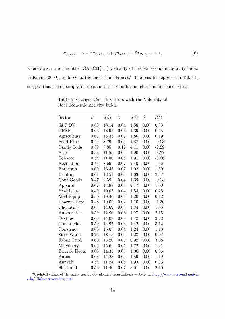
σstock,t = α + βσstock,t−1 + γσoil,t−1 + δσREA,t−1 + εt (6)

where σREA,t−1 is the fitted GARCH(1,1) volatility of the real economic activity index

in Kilian (2009), updated to the end of our dataset.8 The results, reported in Table 5,

suggest that the oil supply/oil demand distinction has no effect on our conclusions.

Table 5: Granger Causality Tests with the Volatility ofReal Economic Activity Index

Sector β̂ t(β̂) γ̂ t(γ̂) δ̂ t(δ̂)S&P 500 0.60 13.14 0.04 1.58 0.00 0.33CRSP 0.62 13.91 0.03 1.39 0.00 0.55Agriculture 0.65 15.43 0.05 1.86 0.00 0.19Food Prod 0.44 8.79 0.04 1.88 0.00 -0.03Candy Soda 0.39 7.85 0.12 4.11 0.00 -2.29Beer 0.53 11.55 0.04 1.90 0.00 -2.37Tobacco 0.54 11.80 0.05 1.91 0.00 -2.66Recreation 0.43 8.69 0.07 2.40 0.00 1.36Entertain 0.60 13.45 0.07 1.92 0.00 1.69Printing 0.61 13.51 0.04 1.63 0.00 2.47Cons Goods 0.47 9.59 0.04 1.69 0.00 -0.13Apparel 0.62 13.93 0.05 2.17 0.00 1.00Healthcare 0.49 10.07 0.04 1.54 0.00 0.25Med Equip 0.50 10.46 0.03 1.20 0.00 0.12Pharma Prod 0.48 10.02 0.02 1.10 0.00 -1.30Chemicals 0.65 14.69 0.03 1.34 0.00 1.05Rubber Plas 0.59 12.96 0.03 1.27 0.00 2.15Textiles 0.62 14.08 0.05 1.72 0.00 3.22Constr Mat 0.59 12.97 0.03 1.42 0.00 3.12Construct 0.68 16.07 0.04 1.24 0.00 1.13Steel Works 0.72 18.15 0.04 1.23 0.00 0.97Fabric Prod 0.60 13.20 0.02 0.92 0.00 3.08Machinery 0.66 15.69 0.05 1.72 0.00 1.21Electric Equip 0.63 14.35 0.05 1.96 0.00 0.56Autos 0.63 14.23 0.04 1.59 0.00 1.19Aircraft 0.54 11.24 0.05 1.93 0.00 0.35Shipbuild 0.52 11.40 0.07 3.01 0.00 2.10

8Updated values of the index can be downloaded from Kilian’s website at http://www-personal.umich.edu/~lkilian/reaupdate.txt.

14

Sector β̂ t(β̂) γ̂ t(γ̂) δ̂ t(δ̂)Defense 0.55 11.66 0.04 1.59 0.00 -0.40Prec Metals 0.63 14.54 0.02 0.50 0.00 0.10Mining 0.77 20.25 0.01 0.26 0.00 1.03Coal 0.81 23.33 0.02 0.67 0.00 0.40Petroleum 0.66 15.27 0.03 1.32 0.00 0.21Utilities 0.59 13.23 0.04 1.84 0.00 0.32Communic 0.65 14.92 0.03 1.32 0.00 -0.59Pers Serv 0.50 10.20 0.04 1.81 0.00 1.71Bus Serv 0.61 13.53 0.03 1.46 0.00 0.91Computers 0.70 18.14 0.02 0.82 0.00 -1.40Comp Soft 0.56 12.40 0.04 1.28 0.00 -2.19Electro Equip 0.73 19.69 0.03 0.90 0.00 -1.62Meas Control 0.74 19.80 0.03 1.20 0.00 -0.42Bus Suppl 0.57 12.33 0.03 1.53 0.00 1.30Ship Cont 0.50 10.64 0.06 2.24 0.00 -0.08Transport 0.51 10.59 0.04 1.71 0.00 1.76Wholesale 0.58 12.49 0.04 1.93 0.00 1.40Retail 0.59 13.26 0.03 1.45 0.00 -1.21Rest Hotels 0.51 10.72 0.05 2.57 0.00 -0.26Banking 0.75 19.37 0.06 1.75 0.00 1.16Insurance 0.71 17.08 0.04 1.44 0.00 1.02Real Estate 0.74 19.30 0.04 1.45 0.00 1.73Trading 0.79 21.87 0.02 0.67 0.00 -0.08Others 0.57 12.30 0.05 1.58 0.00 -0.05

4 Parameter Stability

A central concern when forecasting is that the parameters of the model should be stable

over time (see e.g. Clark & McCracken, 2013). There are two reasons to be concerned

about parameter instability with the stock return volatility-oil price volatility relationship

in particular. First, a one-time event like the U.S. financial crisis could make it harder

to find evidence of predictability in the full sample (due to outlier behavior) or easier

(if there was a strong correlation between the variables only during the crisis). Second,

the price of oil is driven by multiple shocks, including oil supply and aggregate demand

15

shocks, and the relative importance of those shocks will change over time. A Granger

causality test using the full sample might reject γ = 0 in equation (4), even though oil

price volatility is not useful as a predictor of stock return volatility, or vice versa.

To get an overview of the degree of stability of the coefficient estimates, Figure 3 presents

plots of 10-year rolling window estimates of γ in equation (4) for the S&P 500 and CRSP.

The estimates of γ follow similar patterns for the two indices. For the subsamples that

end before 2001, γ̂ is about zero. γ̂ is negative and falling for the samples ending in the

period 2003-2005. In 2008, after the fall of Lehmann Brothers, and at a time of extreme

volatility of oil prices and stock returns, γ̂ jumped sharply. The variation in the parameter

estimates over time is so great that it is possible to find evidence for any desired correlation

- positive, negative, or zero - by simply choosing an appropriate window of data. This

calls into question the reliability of Granger causality tests as a tool for evaluating the

usefulness of oil price volatility as a predictor of stock return volatility.

We repeated the above exercise for each of the 49 industry portfolios. The results are

summarized in Table 6, with the S&P 500 and CRSP included for comparison purposes.

For each industry portfolio, we report the smallest γ̂, the largest γ̂, and the p-value for the

sup-F test of Andrews (1993) for a structural break at an unknown date. Our findings for

the S&P 500 and CRSP indices carry through to all of the sectors, with γ̂ changing signs

in all but four cases, and even for those four industries, the estimates of γ cover a range

of similar width to the estimates for the S&P 500. The null hypothesis of no structural

break is rejected for every return volatility series. This is further evidence that Granger

causality test results for the full sample are not a reliable way to assess the usefulness of

oil price volatility as a predictor of stock return volatility.

16

a: S&P 500

Sample End Date

2000 2005 2010 2015

−0.

050.

000.

050.

10

Est

imat

e of

γ

b: CRSP

Sample End Date

2000 2005 2010 2015

−0.

050.

000.

050.

100.

15

Est

imat

e of

γ

Figure 3: Rolling Window Estimates

17

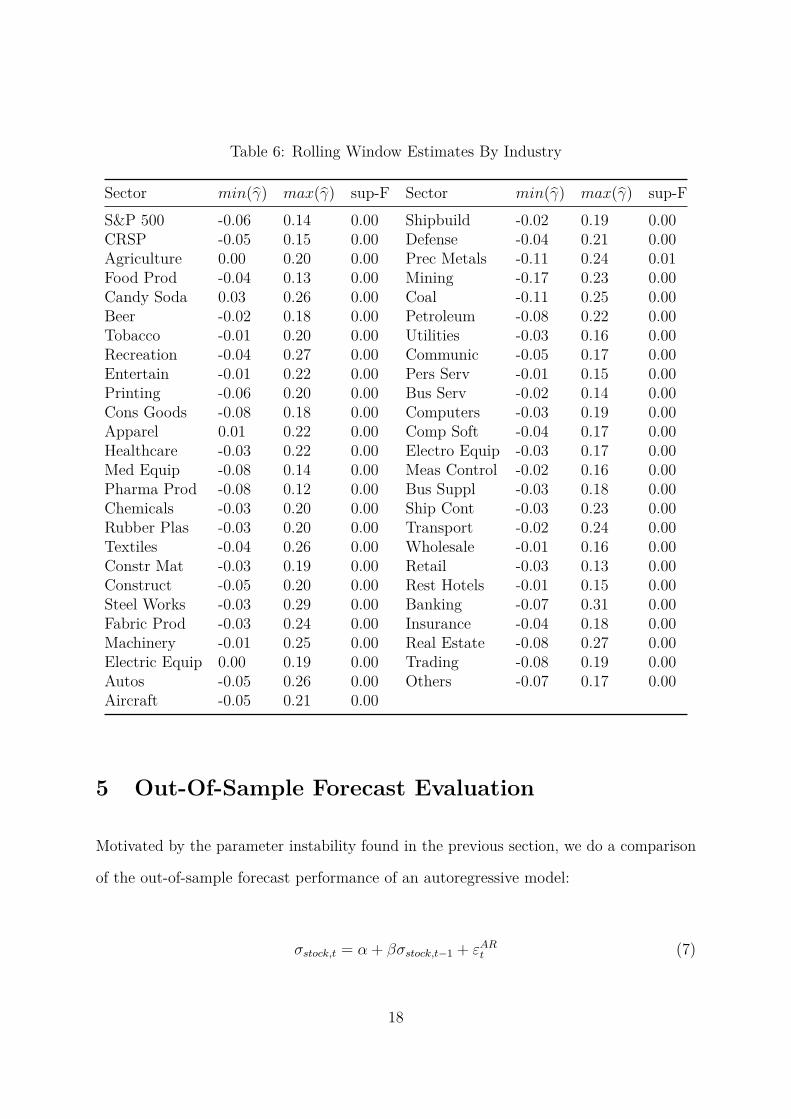
Table 6: Rolling Window Estimates By Industry

Sector min(γ̂) max(γ̂) sup-F Sector min(γ̂) max(γ̂) sup-FS&P 500 -0.06 0.14 0.00 Shipbuild -0.02 0.19 0.00CRSP -0.05 0.15 0.00 Defense -0.04 0.21 0.00Agriculture 0.00 0.20 0.00 Prec Metals -0.11 0.24 0.01Food Prod -0.04 0.13 0.00 Mining -0.17 0.23 0.00Candy Soda 0.03 0.26 0.00 Coal -0.11 0.25 0.00Beer -0.02 0.18 0.00 Petroleum -0.08 0.22 0.00Tobacco -0.01 0.20 0.00 Utilities -0.03 0.16 0.00Recreation -0.04 0.27 0.00 Communic -0.05 0.17 0.00Entertain -0.01 0.22 0.00 Pers Serv -0.01 0.15 0.00Printing -0.06 0.20 0.00 Bus Serv -0.02 0.14 0.00Cons Goods -0.08 0.18 0.00 Computers -0.03 0.19 0.00Apparel 0.01 0.22 0.00 Comp Soft -0.04 0.17 0.00Healthcare -0.03 0.22 0.00 Electro Equip -0.03 0.17 0.00Med Equip -0.08 0.14 0.00 Meas Control -0.02 0.16 0.00Pharma Prod -0.08 0.12 0.00 Bus Suppl -0.03 0.18 0.00Chemicals -0.03 0.20 0.00 Ship Cont -0.03 0.23 0.00Rubber Plas -0.03 0.20 0.00 Transport -0.02 0.24 0.00Textiles -0.04 0.26 0.00 Wholesale -0.01 0.16 0.00Constr Mat -0.03 0.19 0.00 Retail -0.03 0.13 0.00Construct -0.05 0.20 0.00 Rest Hotels -0.01 0.15 0.00Steel Works -0.03 0.29 0.00 Banking -0.07 0.31 0.00Fabric Prod -0.03 0.24 0.00 Insurance -0.04 0.18 0.00Machinery -0.01 0.25 0.00 Real Estate -0.08 0.27 0.00Electric Equip 0.00 0.19 0.00 Trading -0.08 0.19 0.00Autos -0.05 0.26 0.00 Others -0.07 0.17 0.00Aircraft -0.05 0.21 0.00

5 Out-Of-Sample Forecast Evaluation

Motivated by the parameter instability found in the previous section, we do a comparison

of the out-of-sample forecast performance of an autoregressive model:

σstock,t = α + βσstock,t−1 + εARt (7)

18

against that of an ARX model that includes lagged oil price volatility:9

σstock,t = α + βσstock,t−1 + γσoil,t−1 + εARXt (8)

We split the sample into an initial estimation period of January 1986 to December 1999,

and a validation period of January 2000 to April 2015. The two models were estimated

recursively, using all data that would have been available at the time a forecast was made.

To make the initial forecasts, both models were estimated using data from January 1986 to

December 1999, and the estimated models were used to make forecasts of σstock in January

2000. The dataset was updated to include data through January 2000, the two models

were reestimated, and forecasts were made of σstock in February 2000. The process was

repeated until forecasts of σstock were produced for all 184 observations in the validation

period.

5.1 How Different Are In-Sample and Out-Of-Sample Fore-

casts?

We begin by asking how different the in-sample and out-of-sample stock return volatility

forecasts are. On one hand, it is more convenient to do inference on in-sample predictions.

In practice, however, all stock return forecasts are by definition made in an out-of-sample

fashion, so it is only reasonable to draw conclusions from in-sample analysis if the two

methods produce forecasts that are about the same. One metric for measuring the

quality of approximation provided by in-sample forecasts is the mean absolute percentage

difference in the forecasts:9This is equivalent to a vector autoregressive forecast of stock return volatility.

19

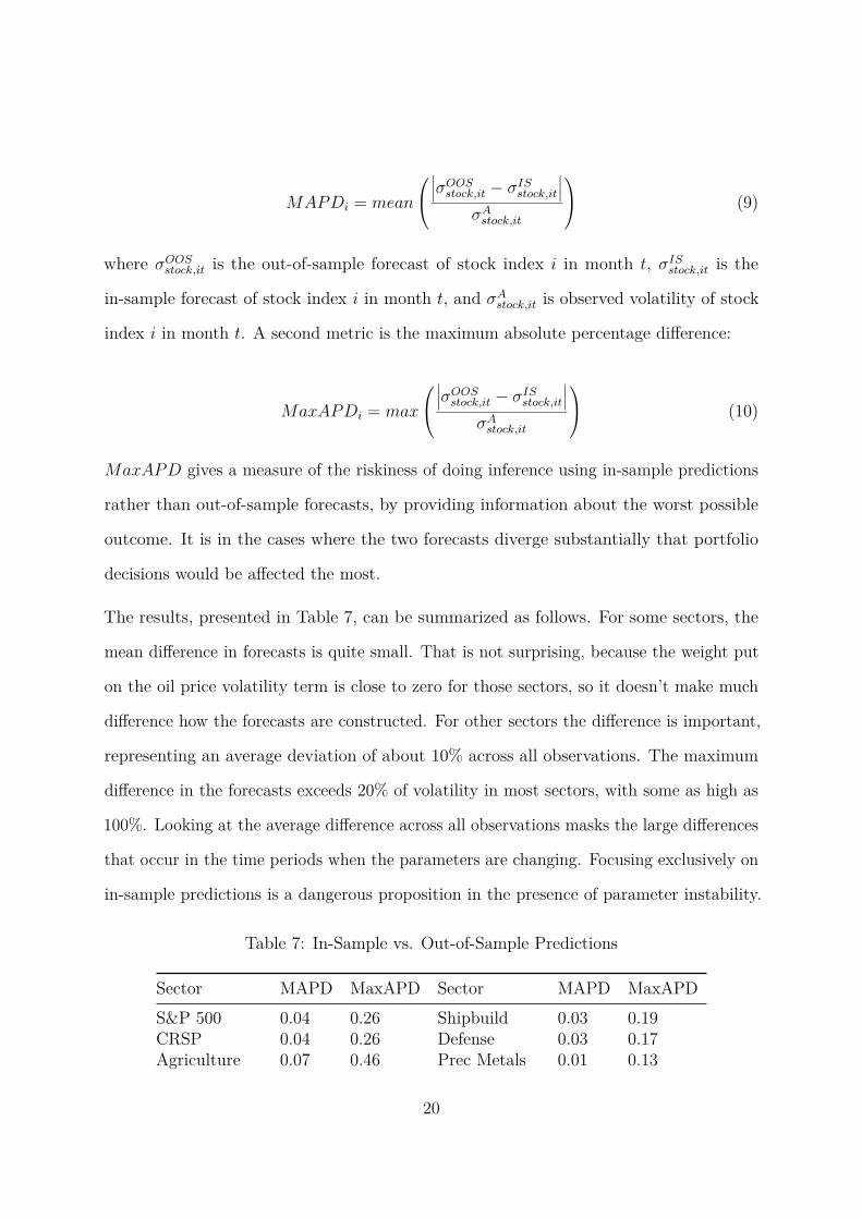
MAPDi = mean

∣∣∣σOOS

stock,it − σISstock,it

∣∣∣σA

stock,it

(9)

where σOOSstock,it is the out-of-sample forecast of stock index i in month t, σIS

stock,it is the

in-sample forecast of stock index i in month t, and σAstock,it is observed volatility of stock

index i in month t. A second metric is the maximum absolute percentage difference:

MaxAPDi = max

∣∣∣σOOS

stock,it − σISstock,it

∣∣∣σA

stock,it

(10)

MaxAPD gives a measure of the riskiness of doing inference using in-sample predictions

rather than out-of-sample forecasts, by providing information about the worst possible

outcome. It is in the cases where the two forecasts diverge substantially that portfolio

decisions would be affected the most.

The results, presented in Table 7, can be summarized as follows. For some sectors, the

mean difference in forecasts is quite small. That is not surprising, because the weight put

on the oil price volatility term is close to zero for those sectors, so it doesn’t make much

difference how the forecasts are constructed. For other sectors the difference is important,

representing an average deviation of about 10% across all observations. The maximum

difference in the forecasts exceeds 20% of volatility in most sectors, with some as high as

100%. Looking at the average difference across all observations masks the large differences

that occur in the time periods when the parameters are changing. Focusing exclusively on

in-sample predictions is a dangerous proposition in the presence of parameter instability.

Table 7: In-Sample vs. Out-of-Sample Predictions

Sector MAPD MaxAPD Sector MAPD MaxAPDS&P 500 0.04 0.26 Shipbuild 0.03 0.19CRSP 0.04 0.26 Defense 0.03 0.17Agriculture 0.07 0.46 Prec Metals 0.01 0.13

20

Sector MAPD MaxAPD Sector MAPD MaxAPDFood Prod 0.04 0.17 Mining 0.09 0.40Candy Soda 0.07 0.41 Coal 0.03 0.14Beer 0.08 0.38 Petroleum 0.04 0.21Tobacco 0.06 0.25 Utilities 0.06 0.61Recreation 0.03 0.21 Communic 0.05 0.31Entertain 0.05 0.42 Pers Serv 0.04 0.21Printing 0.05 0.52 Bus Serv 0.04 0.27Cons Goods 0.04 0.22 Computers 0.03 0.24Apparel 0.03 0.21 Comp Soft 0.07 0.33Healthcare 0.04 0.22 Electro Equip 0.03 0.29Med Equip 0.04 0.18 Meas Control 0.02 0.24Pharma Prod 0.05 0.18 Bus Suppl 0.04 0.24Chemicals 0.05 0.35 Ship Cont 0.04 0.25Rubber Plas 0.06 0.37 Transport 0.06 0.58Textiles 0.09 1.01 Wholesale 0.04 0.35Constr Mat 0.06 0.55 Retail 0.03 0.13Construct 0.06 0.28 Rest Hotels 0.03 0.22Steel Works 0.06 0.47 Banking 0.06 0.31Fabric Prod 0.07 0.46 Insurance 0.07 0.46Machinery 0.05 0.29 Real Estate 0.09 0.57Electric Equip 0.03 0.17 Trading 0.03 0.14Autos 0.06 0.57 Others 0.06 0.33Aircraft 0.03 0.21

5.2 Forecast Evaluation Results

Letting σ̂stock,it be the out-of-sample forecast of stock return volatility from model i in

month t, the out-of-sample forecast error for model i in month t, eit, can be calculated as

eit = σstock,t − σ̂stock,it (11)

The forecast errors for the two models (scaled by 1000 for readability) can be found in

Figure 4. The two series are so similar as to be almost indistinguishable. There is no

21

obvious advantage to using one or the other of the models based on Figure 4.

For

ecas

t Err

or

2000 2005 2010 2015

010

20

Figure 4: Out-of-Sample Forecast Errors

Following Diebold and Mariano (1995), a common approach to comparing forecasting

models is to calculate the loss differential series. For our models, assuming MSE loss, the

loss differential series is

dt = e2AR,t − e2

ARX,t (12)

A positive value of dt indicates that the forecast loss associated with the month t AR

model forecast was greater, a negative value indicates that the ARX model forecast loss

was greater, and a value of zero indicates that the models forecast equally well. Figure 5

is a plot of the loss differential series. It is in most cases small relative to the squared

forecast errors and there is no obvious tendency for it to be positive.10 The pattern of

the loss differential series in Figure 5 suggests that the financial crisis and the period10The loss differential series is positive (a smaller loss associated with the ARX model forecast) 55% of

the time. The MSE for the ARX model is 23.2, the MSE for the AR model is 23.4, and the MSE ratiofor the two models is 0.99.

22

that followed may have been different from the rest of the sample. We accommodate this

by using dummies to allow the relative forecast performance of the two models to be

different during the crisis period.

Diff

eren

ce In

For

ecas

t Los

s

2000 2005 2010 2015

−10

−5

05

1015

Figure 5: Forecast Loss Differential Series

In Table 8 are estimates of the regressions

dt = α + εt (13)

dt = α + β1I1t + εt (14)

dt = α + β1I1t + β2I2t + εt (15)

where I1t = 1 in the period 2008-2009 and zero otherwise, and I2t = 1 in the period

2010-2011 and zero otherwise.

23

Table 8: Loss Differential Across Subsamples

Eq. 13 Eq. 14 Eq. 15α 0.19 0.07 0.13t(α) 1.49 0.51 0.88

β1 0.95 0.89t(β1) 2.51 2.32

β2 -0.41t(β2) -1.06

The estimates in column 1 of Table 8 confirm that the AR model has a larger MSE for the

full out-of-sample period. The estimates in columns 2 and 3 suggest that the difference in

MSE is driven largely by the 2008-2009 time period, in the immediate aftermath of the

financial crisis, when stock returns and oil prices were experiencing high volatility.

A Diebold and Mariano (DM: 1995) comparison of the models could be done using the

estimates of α in Table 8. The downside of that approach is that the distribution of

the DM statistic is nonstandard when the models are nested. We instead apply the

ENC-NEW test of Clark and McCracken (2001) to test the null hypothesis that the two

models forecast equally well against the alternative that the ARX model forecasts have a

lower MSE. We do the test for the S&P 500, CRSP, and each of the 49 industry portfolios.

The AIC and SIC select a lag length of one, but to confirm that our results are not

sensitive to this choice, we also report results for a lag length of two. The tabulated 95%

critical values provided in Clark and McCracken (2001) are 2.234 for one lag and 2.709

for two lags.

The ENC-NEW test statistics can be found in Table 9. The columns titled “Full Sample”

report the ENC-NEW statistic calculated using the full out-of-sample period. Five

industries have test statistics greater than the critical value of 2.234: Candy and Soda,

Recreation, Shipbuilding, Shipping Containers, and Restaurants and Hotels. As shown in

24

the previous section, however, the 2008-2009 time period was one in which both volatility

series were larger than normal due to the U.S. financial crisis, and there is evidence of

parameter instability as a result. Therefore, the evidence that oil price volatility is useful

as a predictor of stock return volatility for these industries can be called into question.

The columns titled “1 Lag” and “2 Lag” are the ENC-NEW statistics calculated by

dropping the forecasts for the 2008-2009 time period. Dropping those observations causes

the ENC-NEW test statistics to drop in nearly all cases. The only industry for which we

can reject the null hypothesis is Candy and Soda. Our results cannot be attributed to the

use of an overly parsimonious model, as we are not able to reject the null hypothesis for

any of the industries when using a longer lag length.

Except for the Candy and Soda industry, stock return volatility forecasts cannot be

improved by accounting for oil price volatility. The relationship is plagued by instabilities

following from the greater volatility of the financial crisis period.

25

Table 9: ENC-NEW Test Statistics By Industry

Sector Full Sample 1 Lag 2 Lags Sector Full Sample 1 Lag 2 LagsS&P 500 0.93 0.52 0.20 Shipbuild 3.44 -1.28 -0.78CRSP 0.51 0.21 -0.06 Defense 0.80 0.42 0.54Agriculture 0.56 -0.50 -0.31 Prec Metals -1.94 -0.89 -0.15Food Prod 1.48 1.02 0.72 Mining -0.86 0.20 0.14Candy Soda 7.33 3.12 1.35 Coal -0.28 -0.11 -0.15Beer 0.81 0.88 0.61 Petroleum -0.14 -0.16 0.06Tobacco 1.09 0.89 0.38 Utilities 0.33 0.17 0.11Recreation 3.20 1.28 1.84 Communic 0.12 0.29 0.02Entertain 1.18 -0.21 -0.35 Pers Serv 1.20 -0.11 -0.39Printing 0.32 0.01 -0.27 Bus Serv 0.60 0.09 -0.14Cons Goods 1.10 0.76 0.65 Computers -0.39 -0.36 0.04Apparel 1.65 0.40 -0.39 Comp Soft -0.29 -0.21 0.17Healthcare -0.09 -0.69 0.46 Electro Equip -0.23 -0.18 -0.01Med Equip -0.25 0.45 1.05 Meas Control 0.16 0.08 0.01Pharma Prod -0.13 0.54 0.53 Bus Suppl 0.39 0.22 0.18Chemicals 0.22 -0.25 -0.37 Ship Cont 2.26 0.92 0.55Rubber Plas 0.00 -0.24 -0.29 Transport 0.56 -0.05 0.20Textiles 0.53 -0.72 -1.00 Wholesale 1.02 -0.05 -0.40Constr Mat 0.26 -0.87 -1.05 Retail 0.63 0.48 -0.05Construct 0.27 -0.57 -0.34 Rest Hotels 3.12 1.29 0.81Steel Works -0.12 -0.39 -0.07 Banking 0.64 -0.30 -0.25Fabric Prod -0.42 -0.59 -0.42 Insurance 0.42 0.01 -0.06Machinery 0.74 -0.18 -0.23 Real Estate 0.13 -0.19 0.34Electric Equip 1.44 0.42 0.07 Trading -0.03 -0.10 -0.32Autos 0.52 -0.04 -0.01 Others 0.97 0.31 0.39Aircraft 1.00 0.26 0.27

6 Conclusions

This paper has revisited the question of whether oil price volatility is useful as a predictor

of stock price volatility. There is a strong, positive contemporaneous relationship between

the two volatility series. Consistent with previous studies, there is clear evidence of a

predictive relationship when doing inference on the full sample.

The results are different when we evaluate of the ability of oil price volatility to improve

26

out-of-sample forecasts of stock return volatility. Formal out-of-sample predictive ability

tests find no evidence that oil price volatility can be used to improve forecasts of stock

return volatility.11 Further investigation reveals that the relationship between the two

volatility series fluctuates wildly through time.12 The changes in the relationship are

not just in magnitude, but also in sign. One could find a strong positive relationship, a

strong negative relationship, or no relationship at all, simply by choosing an appropriate

subsample. Therefore, in spite of the reasonableness of the argument that there should

be a link between stock market volatility and oil market volatility, we conclude that it

cannot be exploited in practice.13

Our results provide no support for the hypothesis that oil price volatility should be used

as a predictor of stock return volatility. Thus, monetary and fiscal policy authorities

should not adjust policy in response to high oil price volatility, unless there are other

concerns about oil price volatility beyond the effects on stock price volatility.

Acknowledgments

We thank the anonymous reviewer for the insightful comments and suggestions.

References

Alsalman, Z., & Herrera, A. M. (2015). Oil Price Shocks and the U.S. Stock Market: Do

Sign and Size Matter? The Energy Journal, 36 (3), 171–188.

Andersen, T. G., Bollerslev, T., Diebold, F. X., & Labys, P. (2003). Modeling and11Further analysis (results are available upon request) showed that our out-of-sample forecast findings

are not sensitive to the choice of time period.12Note that we are referring here to a forecasting relationship, not a conditional correlation.13We repeated the analysis using Brent spot prices. The results, available upon request, do not change

any of our conclusions.

27

Forecasting Realized Volatility. Econometrica, 71 (2), 579–625.

Andrews, D. W. K. (1993). Tests for Parameter Instability and Structural Change with

Unknown Change Point. Econometrica, 61 (4), 821–856.

Apergis, N., & Miller, S. M. (2009). Do Structural Oil-Market Shocks Affect Stock Prices?

Energy Economics, 31 (4), 569–575.

Atems, B., Kapper, D., & Lam, E. (2015). Do Exchange Rates Respond Asymmetrically

to Shocks in the Crude Oil Market? Energy Economics, 49, 227–238.

Basher, S. A., Haug, A. A., & Sadorsky, P. (2012). Oil Prices, Exchange Rates and

Emerging Stock Markets. Energy Economics, 34 (1), 227–240.

Chen, S. (2010). Do Higher Oil Prices Push the Stock Market into Bear Territory? Energy

Economics, 32 (2), 490–495.

Clark, T. E., & McCracken, M. W. (2001). Tests of Equal Forecast Accuracy and

Encompassing for Nested Models. Journal of Econometrics, 105, 85–110.

Clark, T. E., & McCracken, M. W. (2013). Advances in Forecast Evaluation. Handbook

of Economic Forecasting (Vol. 2). Amsterdam: North Holland.

Cunado, J., & De Gracia, F. P. (2014). Oil Price Shocks and Stock Market Returns:

Evidence for Some European Countries. Energy Economics, 42, 365–377.

Den Haan, W. J. (2000). The Comovement Between Output and Prices. Journal of

Monetary Economics, 46 (1), 3–30.

Diebold, F. X., & Mariano, R. S. (1995). Comparing Predictive Accuracy. Journal of

Business and Economic Statistics, 13 (3), 253–263.

Driesprong, G., Jacobsen, B., & Maat, B. (2008). Striking Oil: Another Puzzle? Journal

of Financial Economics, 89 (2), 307–327.

Edelstein, P., & Kilian, L. (2009). How Sensitive are Consumer Expenditures to Retail

28

Energy Prices? Journal of Monetary Economics, 56 (6), 766–779.

Elyasiani, E., Mansur, I., & Odusami, B. (2011). Oil Price Shocks and Industry Stock

Returns. Energy Economics, 33 (5), 966–974.

Farmer, R. E. A. (2012). The Stock Market Crash of 2008 Caused the Great Recession:

Theory and Evidence. Journal of Economic Dynamics and Control, 36 (5), 693–707.

Gicheva, D., Hastings, J., & Villas-Boas, S. (2010). Investigating Income Effects in

Scanner Data: Do Gasoline Prices Affect Grocery Purchases? American Economic Review,

100 (2), 480–484.

Hamilton, J. D. (1994). Time Series Analysis (Vol. 2). Princeton, NJ: Princeton

University Press.

Hamilton, J. D. (2011). Nonlinearities and the Macroeconomic Effects of Oil Prices.

Macroeconomic Dynamics, 15 (S5), 364–378.

Hammoudeh, S., Dibooglu, S., & Aleisa, E. (2004). Relationships Among U.S. Oil Prices

and Oil Industry Equity Indices. International Review of Economics & Finance, 13 (4),

427–453.

Herrera, A. M., & Pesavento, E. (2009). Oil Price Shocks, Systematic Monetary Policy

and the ”Great Moderation”. Macroeconomic Dynamics, 13 (1), 107–137.

Herrera, A. M., Lagalo, L. G., & Wada, T. (2011). Oil Price Shocks and Industrial

Production: Is the Relationship Linear? Macroeconomic Dynamics, 15 (S3), 472–497.

Jones, C. M., & Kaul, G. (1996). Oil and the Stock Markets. Journal of Finance, 51 (2),

463–491.

Kilian, L. (2009). Not All Oil Price Shocks Are Alike: Disentangling Demand and Supply

Shocks in the Crude Oil Market. American Economic Review, 99 (3), 1053–1069.

Kilian, L., & Park, C. (2009). The Impact of Oil Price Shocks on the U.S. Stock Market.

29

International Economic Review, 50 (4), 1267–1287.

Kilian, L., & Lewis, L. T. (2010). Does the Fed Respond to Oil Price Shocks? The

Economic Journal, 121 (555), 1047–1072.

Kilian, L., & Vigfusson, R. J. (2011). Are the Responses of the U.S. Economy Asymmetric

in Energy Price Increases and Decreases? Quantitative Economics, 2 (3), 419–453.

Melichar, M. (2016). Energy Price Shocks and Economic Activity: Which Energy Price

Series Should We Be Using? Energy Economics, 54, 431–443.

Pettenuzzo, D., & Timmerman, A. (2011). Predictability of Stock Returns and Asset

Allocation under Structural Breaks. Journal of Econometrics, 164 (1), 60–78.

Phelps, E. S. (1999). Behind This Structural Boom: The Role of Asset Valuations.

American Economic Review, 89 (2), 63–68.

Sadorsky, P. (1999). Oil Price Shocks and Stock Market Activity. Energy Economics,

21 (5), 449–469.

Sadorsky, P. (2003). The Macroeconomic Determinants of Technology Stock Price Volatil-

ity. Review of Financial Economics, 12 (2), 191–205.

Schwert, W. G. (1989). Why Does Stock Market Volatility Change Over Time? Journal

of Finance, 44 (5), 1115–1153.

30

Not-For-Publication Appendices

Appendix A: Out-Of-Sample Forecast Evaluation

In order to confirm that the out-of-sample forecast evaluation was not driven by the choice

of time period, we repeated the analysis using an initial estimation period of January 1986

to December 2004 and a validation period of January 2005 to April 2015. This sample

split was chosen so that none of the out-of-sample forecasts included the Iraq War.

Table A.1: In-Sample vs. Out-of-Sample Predictions

Sector MAPD MaxAPD Sector MAPD MaxAPDS&P 500 0.03 0.16 Shipbuild 0.02 0.12CRSP 0.02 0.13 Defense 0.02 0.10Agriculture 0.05 0.35 Prec Metals 0.01 0.07Food Prod 0.03 0.17 Mining 0.05 0.34Candy Soda 0.07 0.41 Coal 0.02 0.08Beer 0.06 0.38 Petroleum 0.02 0.19Tobacco 0.06 0.21 Utilities 0.02 0.17Recreation 0.02 0.15 Communic 0.03 0.14Entertain 0.03 0.16 Pers Serv 0.02 0.14Printing 0.03 0.17 Bus Serv 0.01 0.08Cons Goods 0.03 0.18 Computers 0.02 0.05Apparel 0.02 0.15 Comp Soft 0.06 0.33Healthcare 0.03 0.18 Electro Equip 0.02 0.06Med Equip 0.03 0.17 Meas Control 0.01 0.04Pharma Prod 0.04 0.18 Bus Suppl 0.02 0.11Chemicals 0.02 0.17 Ship Cont 0.03 0.16Rubber Plas 0.03 0.16 Transport 0.03 0.19Textiles 0.04 0.34 Wholesale 0.02 0.11Constr Mat 0.04 0.24 Retail 0.02 0.09Construct 0.03 0.17 Rest Hotels 0.02 0.14Steel Works 0.03 0.17 Banking 0.04 0.25Fabric Prod 0.04 0.46 Insurance 0.04 0.26Machinery 0.02 0.13 Real Estate 0.07 0.42Electric Equip 0.02 0.13 Trading 0.02 0.06Autos 0.04 0.20 Others 0.05 0.26Aircraft 0.02 0.07

31

For

ecas

t Err

or

2006 2008 2010 2012 2014

010

20

Figure A.1: Out-of-Sample Forecast Errors

32

Diff

eren

ce In

For

ecas

t Los

s

2006 2008 2010 2012 2014

−10

−5

05

1015

Figure A.2: Forecast Loss Differential Series

Table A.2: Loss Differential Across Subsamples

Eq. 13 Eq. 14 Eq. 15α 0.31 0.14 0.27t(α) 1.65 0.67 1.14

β1 0.88 0.75t(β1) 1.86 1.54

β2 -0.55t(β2) -1.12

33

Table A.3: ENC-NEW Test Statistics By Industry

Sector Full Sample 1 Lag 2 Lags Sector Full Sample 1 Lag 2 LagsS&P 500 0.91 0.72 0.58 Shipbuild 3.07 -1.36 -1.16CRSP 0.55 0.36 0.28 Defense 1.25 1.12 1.36Agriculture 0.28 -0.88 -0.30 Prec Metals -1.39 -0.27 -0.06Food Prod 1.67 1.56 1.50 Mining -0.70 0.12 0.14Candy Soda 8.48 3.42 1.87 Coal -0.22 -0.02 -0.18Beer 0.96 1.37 1.26 Petroleum -0.06 -0.02 0.06Tobacco 1.68 1.84 0.85 Utilities 0.49 0.67 0.27Recreation 3.00 1.54 2.53 Communic 0.19 0.65 0.44Entertain 1.50 -0.31 -0.23 Pers Serv 1.06 -0.11 -0.32Printing 0.39 0.14 0.00 Bus Serv 0.79 0.30 0.24Cons Goods 1.64 1.79 2.10 Computers 0.08 0.18 0.20Apparel 1.44 0.35 -0.20 Comp Soft 0.29 0.58 0.53Healthcare 0.54 -0.19 0.94 Electro Equip 0.15 0.35 0.24Med Equip -0.47 0.23 1.35 Meas Control 0.30 0.26 0.24Pharma Prod -0.36 0.44 0.89 Bus Suppl 0.49 0.44 0.30Chemicals 0.30 -0.13 -0.20 Ship Cont 2.29 1.25 0.81Rubber Plas 0.03 -0.20 -0.25 Transport 0.83 0.39 0.38Textiles 0.63 -0.99 -1.34 Wholesale 1.13 -0.02 -0.39Constr Mat 0.26 -0.82 -0.85 Retail 0.84 0.89 0.72Construct 0.31 -0.43 -0.27 Rest Hotels 3.13 1.58 1.41Steel Works 0.07 -0.15 0.01 Banking 0.64 0.02 -0.03Fabric Prod -0.29 -0.46 -0.27 Insurance 0.44 0.15 0.10Machinery 0.78 -0.16 -0.20 Real Estate 0.10 -0.12 0.15Electric Equip 1.51 0.60 0.30 Trading 0.06 0.04 -0.13Autos 0.57 0.05 0.03 Others 1.46 0.94 1.17Aircraft 1.83 1.15 0.86

Appendix B: Robustness Checks Using Brent Spot Prices

In order to confirm that our results are not specific to the choice of WTI as the oil price

series, we repeated the analysis using daily data on Brent spot prices over the period

June 1, 1987 to April 30, 2015. Brent spot prices are available from the Federal Reserve

Economic Database (FRED).

34

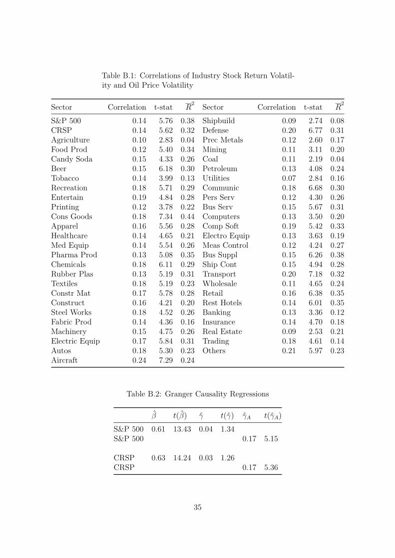
Table B.1: Correlations of Industry Stock Return Volatil-ity and Oil Price Volatility

Sector Correlation t-stat R2 Sector Correlation t-stat R

2

S&P 500 0.14 5.76 0.38 Shipbuild 0.09 2.74 0.08CRSP 0.14 5.62 0.32 Defense 0.20 6.77 0.31Agriculture 0.10 2.83 0.04 Prec Metals 0.12 2.60 0.17Food Prod 0.12 5.40 0.34 Mining 0.11 3.11 0.20Candy Soda 0.15 4.33 0.26 Coal 0.11 2.19 0.04Beer 0.15 6.18 0.30 Petroleum 0.13 4.08 0.24Tobacco 0.14 3.99 0.13 Utilities 0.07 2.84 0.16Recreation 0.18 5.71 0.29 Communic 0.18 6.68 0.30Entertain 0.19 4.84 0.28 Pers Serv 0.12 4.30 0.26Printing 0.12 3.78 0.22 Bus Serv 0.15 5.67 0.31Cons Goods 0.18 7.34 0.44 Computers 0.13 3.50 0.20Apparel 0.16 5.56 0.28 Comp Soft 0.19 5.42 0.33Healthcare 0.14 4.65 0.21 Electro Equip 0.13 3.63 0.19Med Equip 0.14 5.54 0.26 Meas Control 0.12 4.24 0.27Pharma Prod 0.13 5.08 0.35 Bus Suppl 0.15 6.26 0.38Chemicals 0.18 6.11 0.29 Ship Cont 0.15 4.94 0.28Rubber Plas 0.13 5.19 0.31 Transport 0.20 7.18 0.32Textiles 0.18 5.19 0.23 Wholesale 0.11 4.65 0.24Constr Mat 0.17 5.78 0.28 Retail 0.16 6.38 0.35Construct 0.16 4.21 0.20 Rest Hotels 0.14 6.01 0.35Steel Works 0.18 4.52 0.26 Banking 0.13 3.36 0.12Fabric Prod 0.14 4.36 0.16 Insurance 0.14 4.70 0.18Machinery 0.15 4.75 0.26 Real Estate 0.09 2.53 0.21Electric Equip 0.17 5.84 0.31 Trading 0.18 4.61 0.14Autos 0.18 5.30 0.23 Others 0.21 5.97 0.23Aircraft 0.24 7.29 0.24

Table B.2: Granger Causality Regressions

β̂ t(β̂) γ̂ t(γ̂) γ̂A t(γ̂A)S&P 500 0.61 13.43 0.04 1.34S&P 500 0.17 5.15

CRSP 0.63 14.24 0.03 1.26CRSP 0.17 5.36

35

Table B.3: Granger Causality Tests

Sector β̂ t(β̂) γ̂ t(γ̂) Sector β̂ t(β̂) γ̂ t(γ̂)Agriculture 0.67 15.92 0.00 0.07 Defense 0.55 11.19 0.05 1.55Food Prod 0.47 9.26 0.03 1.23 Prec Metals 0.63 14.25 0.04 0.92Candy Soda 0.41 7.99 0.13 3.68 Mining 0.79 22.70 -0.01 -0.31Beer 0.55 11.37 0.04 1.58 Coal 0.80 23.86 0.05 1.01Tobacco 0.58 12.66 0.02 0.67 Petroleum 0.67 15.80 0.02 0.65Recreation 0.45 8.90 0.07 2.09 Utilities 0.61 13.76 0.04 1.53Entertain 0.64 14.69 0.04 1.02 Communic 0.65 14.71 0.03 1.07Printing 0.66 15.65 0.05 1.54 Pers Serv 0.53 11.23 0.05 1.70Cons Goods 0.48 9.51 0.03 0.98 Bus Serv 0.63 14.11 0.03 1.05Apparel 0.65 14.65 0.03 1.06 Computers 0.70 17.34 0.05 1.46Healthcare 0.49 9.88 0.04 1.41 Comp Soft 0.57 12.21 0.06 1.47Med Equip 0.52 10.72 0.02 0.91 Electro Equip 0.72 18.54 0.06 1.72Pharma Prod 0.49 10.08 0.02 0.84 Meas Control 0.74 19.70 0.03 0.97Chemicals 0.68 15.75 0.02 0.49 Bus Suppl 0.59 12.77 0.03 1.03Rubber Plas 0.63 14.32 0.02 0.66 Ship Cont 0.51 10.40 0.06 1.80Textiles 0.68 16.38 0.04 1.08 Transport 0.55 11.10 0.03 0.86Constr Mat 0.67 15.55 0.02 0.69 Wholesale 0.61 13.53 0.04 1.47Construct 0.68 16.37 0.06 1.69 Retail 0.60 12.91 0.03 1.15Steel Works 0.73 18.85 0.04 1.07 Rest Hotels 0.52 10.64 0.05 1.87Fabric Prod 0.66 15.35 0.01 0.32 Banking 0.76 20.47 0.07 1.95Machinery 0.67 16.02 0.06 1.81 Insurance 0.73 18.73 0.03 1.06Electric Equip 0.64 14.40 0.05 1.52 Real Estate 0.77 21.67 0.05 1.44Autos 0.65 14.73 0.04 1.09 Trading 0.78 21.45 0.04 0.99Aircraft 0.55 11.14 0.03 0.82 Others 0.56 11.71 0.07 1.92Shipbuild 0.55 12.01 0.07 2.23

36

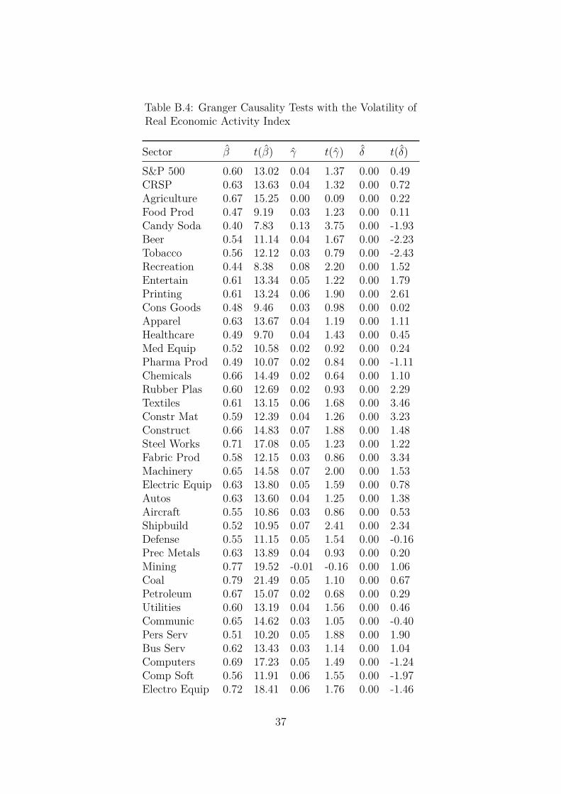
Table B.4: Granger Causality Tests with the Volatility ofReal Economic Activity Index

Sector β̂ t(β̂) γ̂ t(γ̂) δ̂ t(δ̂)S&P 500 0.60 13.02 0.04 1.37 0.00 0.49CRSP 0.63 13.63 0.04 1.32 0.00 0.72Agriculture 0.67 15.25 0.00 0.09 0.00 0.22Food Prod 0.47 9.19 0.03 1.23 0.00 0.11Candy Soda 0.40 7.83 0.13 3.75 0.00 -1.93Beer 0.54 11.14 0.04 1.67 0.00 -2.23Tobacco 0.56 12.12 0.03 0.79 0.00 -2.43Recreation 0.44 8.38 0.08 2.20 0.00 1.52Entertain 0.61 13.34 0.05 1.22 0.00 1.79Printing 0.61 13.24 0.06 1.90 0.00 2.61Cons Goods 0.48 9.46 0.03 0.98 0.00 0.02Apparel 0.63 13.67 0.04 1.19 0.00 1.11Healthcare 0.49 9.70 0.04 1.43 0.00 0.45Med Equip 0.52 10.58 0.02 0.92 0.00 0.24Pharma Prod 0.49 10.07 0.02 0.84 0.00 -1.11Chemicals 0.66 14.49 0.02 0.64 0.00 1.10Rubber Plas 0.60 12.69 0.02 0.93 0.00 2.29Textiles 0.61 13.15 0.06 1.68 0.00 3.46Constr Mat 0.59 12.39 0.04 1.26 0.00 3.23Construct 0.66 14.83 0.07 1.88 0.00 1.48Steel Works 0.71 17.08 0.05 1.23 0.00 1.22Fabric Prod 0.58 12.15 0.03 0.86 0.00 3.34Machinery 0.65 14.58 0.07 2.00 0.00 1.53Electric Equip 0.63 13.80 0.05 1.59 0.00 0.78Autos 0.63 13.60 0.04 1.25 0.00 1.38Aircraft 0.55 10.86 0.03 0.86 0.00 0.53Shipbuild 0.52 10.95 0.07 2.41 0.00 2.34Defense 0.55 11.15 0.05 1.54 0.00 -0.16Prec Metals 0.63 13.89 0.04 0.93 0.00 0.20Mining 0.77 19.52 -0.01 -0.16 0.00 1.06Coal 0.79 21.49 0.05 1.10 0.00 0.67Petroleum 0.67 15.07 0.02 0.68 0.00 0.29Utilities 0.60 13.19 0.04 1.56 0.00 0.46Communic 0.65 14.62 0.03 1.05 0.00 -0.40Pers Serv 0.51 10.20 0.05 1.88 0.00 1.90Bus Serv 0.62 13.43 0.03 1.14 0.00 1.04Computers 0.69 17.23 0.05 1.49 0.00 -1.24Comp Soft 0.56 11.91 0.06 1.55 0.00 -1.97Electro Equip 0.72 18.41 0.06 1.76 0.00 -1.46

37

Sector β̂ t(β̂) γ̂ t(γ̂) δ̂ t(δ̂)Meas Control 0.75 19.58 0.03 0.96 0.00 -0.32Bus Suppl 0.57 11.98 0.03 1.15 0.00 1.42Ship Cont 0.51 10.26 0.06 1.81 0.00 0.21Transport 0.52 10.06 0.03 1.09 0.00 1.95Wholesale 0.59 12.47 0.04 1.63 0.00 1.55Retail 0.60 12.92 0.03 1.15 0.00 -0.98Rest Hotels 0.52 10.56 0.05 1.86 0.00 0.04Banking 0.73 18.40 0.08 2.16 0.00 1.47Insurance 0.72 16.91 0.04 1.22 0.00 1.10Real Estate 0.73 18.34 0.06 1.73 0.00 2.00Trading 0.78 20.54 0.04 1.00 0.00 0.14Others 0.56 11.64 0.07 1.92 0.00 0.16

38

Table B.5: Rolling Window Estimates By Industry

Sector min(γ̂) max(γ̂) sup-F Sector min(γ̂) max(γ̂) sup-FS&P 500 -0.05 0.12 0.00 Shipbuild -0.02 0.13 0.00CRSP -0.03 0.12 0.00 Defense -0.06 0.19 0.00Agriculture -0.08 0.10 0.00 Prec Metals -0.04 0.21 0.01Food Prod -0.06 0.11 0.07 Mining -0.20 0.15 0.00Candy Soda 0.07 0.26 0.00 Coal 0.01 0.22 0.00Beer -0.04 0.14 0.00 Petroleum -0.10 0.12 0.00Tobacco -0.09 0.19 0.00 Utilities -0.01 0.12 0.00Recreation -0.06 0.28 0.03 Communic -0.04 0.14 0.00Entertain -0.06 0.22 0.00 Pers Serv -0.04 0.23 0.00Printing -0.01 0.18 0.00 Bus Serv -0.02 0.11 0.00Cons Goods -0.12 0.12 0.04 Computers -0.04 0.27 0.00Apparel -0.06 0.17 0.00 Comp Soft -0.02 0.19 0.00Healthcare -0.03 0.19 0.00 Electro Equip -0.02 0.25 0.00Med Equip -0.05 0.11 0.06 Meas Control -0.03 0.12 0.00Pharma Prod -0.09 0.10 0.03 Bus Suppl -0.06 0.15 0.00Chemicals -0.11 0.13 0.00 Ship Cont -0.05 0.17 0.00Rubber Plas -0.09 0.18 0.00 Transport -0.09 0.19 0.00Textiles -0.11 0.28 0.00 Wholesale 0.00 0.13 0.00Constr Mat -0.06 0.18 0.00 Retail -0.07 0.12 0.00Construct -0.04 0.22 0.00 Rest Hotels -0.03 0.12 0.00Steel Works -0.02 0.23 0.00 Banking -0.10 0.37 0.00Fabric Prod -0.05 0.18 0.00 Insurance -0.05 0.17 0.00Machinery 0.01 0.21 0.00 Real Estate -0.07 0.26 0.00Electric Equip -0.03 0.15 0.00 Trading -0.09 0.19 0.00Autos -0.13 0.21 0.00 Others -0.09 0.22 0.00Aircraft -0.18 0.16 0.00

39

Table B.6: In-Sample vs. Out-of-Sample Predictions

Sector MAPD MaxAPD Sector MAPD MaxAPDS&P 500 0.04 0.25 Shipbuild 0.03 0.20CRSP 0.04 0.24 Defense 0.03 0.15Agriculture 0.08 0.46 Prec Metals 0.01 0.06Food Prod 0.04 0.16 Mining 0.09 0.38Candy Soda 0.07 0.42 Coal 0.03 0.09Beer 0.08 0.37 Petroleum 0.04 0.21Tobacco 0.06 0.23 Utilities 0.06 0.59Recreation 0.03 0.18 Communic 0.05 0.30Entertain 0.05 0.41 Pers Serv 0.04 0.19Printing 0.05 0.52 Bus Serv 0.04 0.26Cons Goods 0.04 0.16 Computers 0.03 0.24Apparel 0.03 0.20 Comp Soft 0.08 0.32Healthcare 0.04 0.18 Electro Equip 0.03 0.27Med Equip 0.03 0.15 Meas Control 0.02 0.25Pharma Prod 0.04 0.19 Bus Suppl 0.03 0.25Chemicals 0.05 0.33 Ship Cont 0.04 0.21Rubber Plas 0.06 0.37 Transport 0.06 0.58Textiles 0.09 0.98 Wholesale 0.05 0.33Constr Mat 0.06 0.52 Retail 0.03 0.12Construct 0.06 0.28 Rest Hotels 0.04 0.21Steel Works 0.06 0.45 Banking 0.06 0.32Fabric Prod 0.07 0.48 Insurance 0.06 0.46Machinery 0.05 0.29 Real Estate 0.09 0.56Electric Equip 0.03 0.17 Trading 0.03 0.14Autos 0.06 0.57 Others 0.06 0.34Aircraft 0.03 0.22

Table B.7: Loss Differential Across Subsamples

Eq. 13 Eq. 14 Eq. 15α 0.36 0.10 0.17t(α) 2.16 0.57 0.91

β1 2.01 1.94t(β1) 4.26 4.06

β2 -0.47t(β2) -0.99

40

Table B.8: ENC-NEW Test Statistics By Industry

Sector Full Sample 1 Lag 2 Lags Sector Full Sample 1 Lag 2 LagsS&P 500 1.61 0.70 0.96 Shipbuild 2.21 -1.10 -0.47CRSP 1.61 0.78 0.83 Defense 1.29 0.66 1.04Agriculture 0.04 -0.08 -0.50 Prec Metals 0.20 -0.37 0.49Food Prod 2.25 2.02 1.55 Mining 0.37 0.52 0.63Candy Soda 6.97 4.05 3.05 Coal 0.51 0.79 0.61Beer 1.11 1.01 1.34 Petroleum 0.19 -0.17 0.33Tobacco 0.69 0.88 1.51 Utilities 1.63 0.96 1.31Recreation 2.75 1.48 2.52 Communic 0.89 0.71 0.80Entertain 1.40 0.38 0.16 Pers Serv 2.44 -0.04 0.01Printing 1.19 0.01 -0.10 Bus Serv 1.71 0.76 0.37Cons Goods 0.65 0.68 0.70 Computers 1.19 0.78 1.03Apparel 1.25 0.38 0.14 Comp Soft 0.62 0.20 0.13Healthcare 0.87 -0.05 0.33 Electro Equip 1.17 0.78 0.34Med Equip 1.33 1.17 1.34 Meas Control -0.03 -0.26 -0.27Pharma Prod 0.88 1.06 0.63 Bus Suppl 0.77 0.28 0.49Chemicals 0.74 0.06 0.02 Ship Cont 2.31 1.01 1.15Rubber Plas 0.45 0.04 0.23 Transport 0.96 0.69 1.21Textiles 1.46 0.44 0.13 Wholesale 1.97 0.47 0.10Constr Mat 0.99 -0.69 -0.72 Retail 1.51 1.16 0.38Construct 1.26 0.85 1.27 Rest Hotels 2.53 1.61 1.17Steel Works 1.24 1.13 1.05 Banking 1.02 -0.22 0.30Fabric Prod 0.49 0.73 0.66 Insurance 0.82 -0.18 -0.09Machinery 2.03 1.36 0.79 Real Estate 0.81 -0.25 0.00Electric Equip 1.48 0.61 0.76 Trading 0.27 0.15 0.19Autos 0.68 0.44 0.95 Others 1.31 0.30 1.34Aircraft 0.42 0.30 1.04

41