Embed Size (px)
Citation preview

Oil boom, job prospects and schooling decisions : Evidence from
Chad
Mahamat MOUSTAPHA∗
Preliminary version, please do not quote or share
Abstract
This paper examines the effect of oil-induced employment opportunities for natives on secondary
schooling decisions in the oil-rich region of Chad. Using a synthetic control method and a difference-
in-differences approach, I find that these opportunities increased secondary school attendance in
the region. Concerning the mechanism, the results suggest, on the one hand, a decrease in school
dropouts, and on the other hand, that the observed effect does not come from an increase in parental
income but incentives related to employment opportunities. Finally, I find similar results when I use
survey data instead of regional administrative data.
Keywords: Oil boom, Labor market, Education, Economic Development, Africa, Chad.
JEL Classification : I25, J08, N37, Q33
∗PhD Student at Paris Dauphine University-LEDa and UMR Dial, [email protected]
1

1 Introduction
The importance of education in the development process has been widely studied in the economics litera-
ture. It has been shown that a high level of education promotes growth and improves national well-being
(Lucas (1998), Mankiw et al. (1992)). However, despite an increase in the number of children attending
school in recent years, early dropout remains an issue, especially in developing countries (Unesco (2018)).
For instance, secondary school attendance in sub-Saharan Africa was about 38% in 2018, while it turned
around 80% for primary school in the same period. In countries like Niger, the Central African Republic,
and Chad, about 80 percent of children drop out before secondary school. The main obstacles to school
attendance identified in this region are low expected returns to education, social pressure for immediate
income, and lack of educational infrastructure (Unesco (2016)). Therefore, any measures to improve
school infrastructure and the expected education benefits could increase secondary school attendance
and reduce early school dropout. While the role of infrastructure on schooling decisions has been the
subject of numerous articles (Duflo (2001), Akresh et al. (2018)), examining the effects of employment
prospects on demand for education is not straightforward due to the difficulty of identifying differences
in prospects between different individuals. The ideal experiment for estimating the effect of perspective
on the education decision would be to randomly assign the job prospect for some individuals and not for
others and then compare the education decisions between individuals. In the absence of evidence of such
an experience, I exploit the Chadian oil boom, particularly the oil sector employment promotion measures
that provide a quasi-natural experimental setting for estimating the effect of employment opportunities
on education demand.
Chad is an oil-exploiting country since 2004 with the financial support of the World Bank. The
World Bank considers that projects can accelerate poverty reduction and promotes economic development
(Kojucharov (2007)). Nevertheless, the country’s ability to manage oil revenues to achieve this poverty
reduction objective has been a major concern for the Chadian government and its partners involved in
this project. The main fear was that the management of oil revenues would exacerbate existing political
tensions instead of favoring its socio-economic development. To address this concern, a law called law
n o 001/PR/1999 was adopted in 1999. This law aims to ensure greater transparency in the use of
oil revenues. According to this law, the distribution plan for oil revenues (dividends and royalties) is as
follows : 10% goes to future generations, 72% is allocated to capital expenditures, 13.5% to operational
expenses, and the remaining 4.5% is transferred to the oil region. Besides the financial transfer, the oil
region also benefits from labor market-oriented measures, such as employment opportunities in the oil
sector and the priority given to local workers in recruitment.
This article’s identification strategy uses the fact that these labor market-oriented measures only
benefit the oil region. These measures can influence schooling decisions in several ways. First, positively,
as they can increase the demand for education. Indeed, if employment prospects in the petroleum sector
involve skilled workers, the investment returns on education increase, raising the incentive to pursue
education. Second, the prioritization of local workers in hiring can give rise to immediate unskilled job
2

opportunities, making the opportunity costs of staying in school higher. Which one of these two opposing
effects prevails remains an empirical question. In any case, this work-study trade-off is mostly involving
secondary school students. I, therefore, focus on individuals in the 16-18 age group.
This article is closer to both the literature on expected returns and schooling decisions and the
literature on the oil boom and schooling decisions. Studies on the relationship between expected returns
and schooling decisions are not new. The earliest work on this issue dates back to Becker (1964) and his
work on human capital. In this seminal paper, Becker presents education as an investment triggered by
a comparison between current costs and the discounted stream of expected future benefits, primarily in
the form of higher wages. Therefore, individuals may decide to pursue further education if the expected
future gains are more significant than the current opportunity costs. Such a trade-off assumes that the
returns to schooling are known. In most developing countries, however, this is not the case because
of the lack of earnings data and guidance counselors who can provide information on the benefits of
schooling (Manski et al. (1983), Jensen (2010)). As a result, students and their parents are not as well
informed about the benefits of education. The handful of existing studies on developing countries involve
providing information to students or parents and examining the effect of this information on the schooling
decision. These include Nguyen (2008), who conducted a field experiment in Madagascar and showed that
increasing the perceived returns to education strengthens incentives to enroll when agents underestimate
the actual returns. Similarly, using survey data on eighth-grade boys in the Dominican Republic, Jensen
(2010) finds that perceived returns to secondary education are meager, despite high measured returns.
He shows that students in randomly selected schools who received information about actual returns
completed an average of 0.20 to 0.35 more years of schooling over the next four years than those who
did not receive such information. In Mexico, Kaufmann (2014) used data on individuals’ subjective
expectations of returns to understand the huge differences in university enrollment rates between poor
and wealthy individuals. He finds that higher expected returns are required for poor individuals to have
an incentive to attend university, suggesting that they face higher opportunity costs than individuals with
wealthy parents. Finally, Attanasio & Kaufmann (2014) found that expected returns and perceptions of
risk are important determinants of schooling decisions in Mexico. This expected return and the perception
of future risks are essential to consider in Chad. Secondary education remains consistently low in this
country, despite the considerable increase in educational provision(the number of schools increased from
6,104 schools in 2005 to 11,490 schools in 2013). Oil-induced employment opportunities for natives could
change their perception of the future local labor market and hence the expected return to education.
Regarding the relationship between the oil boom and school decisions, very few articles have addressed
this issue. The existing studies are either transnational or focus on the United States and Canada. The
effect of the oil boom on schooling decisions also remains ambiguous. Some articles found a negative
impact, while others found adverse effects. In the first set, for example, Gylfason (2001) in a study of
90 countries showed that the share of natural resources in GDP negatively affects education spending,
expected years of schooling for women, and the gross secondary school enrollment rate. Similarly, Cascio
3

& Narayan (2015) showed that the shale gas boom increased dropout rates among adolescents in several
US states. In the same vein, Kumar (2017) used a synthetic cohort approach to compare cohorts that
attended high school during the pre-and post-boom period in the United States. He showed that the
cohort reaching high school age during the oil boom was about 2 percentage points less likely to have
a college degree by the time they turned 34 to 37 years of age in 2000. Rickman et al. (2017) found
similar results in Montana, North Dakota, and West Virginia, where shale growth has led to considerable
reductions in high school enrollment. More recently, Zuo et al. (2019), using data from 15 US states
with oil and gas production over the period 2000-2013, show that intensive drilling activity hurts student
enrollment in grades 11 and 12. Specifically, they find that one additional oil or gas well drilled per 1,000
core workers results in a 0.24% decline in county-level 11th and 12th-grade enrollment, all else being
equal. Alternatively, other papers argue that oil does not negatively affect schooling and improves school
resources. In this category, we have Emery et al. (2012), which finds, using school-age birth cohorts before,
during, and after the oil boom of the 1970s, that educational attainment did not decline in the Canadian
province of Alberta. In Brazil, Caselli & Michaels (2013) showed that oil revenues increased education
spending, teachers, and classrooms per capita in oil-rich municipalities. Similarly, James (2015), Raimi &
Newell (2014), and Weber et al. (2016) show that the shale oil and gas boom has dramatically increased
spending on education and schooling in some US counties.
This study offers three clear contributions to the literature. First, unlike existing research, which
focuses on the effect of information on actual returns to education on schooling, I assess the impact of
promised jobs on educational decisions in this article. These jobs are more likely to influence education
decisions than information on actual returns to education. Second, to the best of my knowledge, this
study is the first to focus on a country in sub-Saharan Africa. Indeed, the existing literature on the oil
boom and school decisions has focused on countries like the United States or Canada. This article is also
the first to highlight the effect of the Chadian oil project presented as a model for fragile countries rich
in natural resources on education outcomes.
This paper examines how oil-induced employment opportunities for natives have influenced secondary
education decisions in the oil region. I use administrative education data from the Chadian Ministry of
Education. Applying the synthetic control method (SCM) developed by Abadie et al. (2010), I find that
oil-induced employment opportunities for natives have significantly increased the net secondary school
enrollment rate in the oil region compared to its synthetic control. I then perform several placebo tests.
All these tests confirm the robustness of this effect. This result is also robust to the method chosen since
a difference-in-differences (DID) analysis confirms the positive impact found with SCM. The analysis of
transmission mechanisms suggests, on the one hand, a decrease in school dropouts and, on the other
hand, that the observed effect does not come from the increase in parental income but incentives linked
to employment opportunities. I also examined whether the results are linked to a massive migration to
the oil region to take advantage of the oil boom. Population census data show no significant migration to
the oil region from its pre-oil trend. Furthermore, the priority to local workers in the recruitment process
4

mentioned above seems to discourage migration to the oil region. Finally, I obtain similar results using
nationally representative survey data instead of administrative data.
The rest of the paper is organized as follows. Section 2 provides an overview of the program and
education in Chad. The data, the empirical model, and the identification strategy are presented in
Section 3. In section 4, I show the main results. Next, I examine some transmission channels and check
the robustness of the findings in sections 5 and 6 respectively. Finally, section 7 concludes and discusses
the policy implications.
2 Background
I first present the program. Then, I will describe the education system and the educational situation in
Chad.
2.1 The program
2.1.1 Chadian oil project
The Chadian oil story began in 1969 when the Chadian government granted the very first oil exploration
license to the American company Conoco. In 1973, the first oil explorations started in the south of
the country. However, this initial exploration period ended in 1975 with the overthrow of Chad’s first
president, which also marked the departure of Conoco. Another consortium composed of Chevron (20%),
Exxon (40%), and Shell (40%) was set up to continue exploration three years later. However, institutional
instabilities have long disrupted the activities of this consortium.
It was not until 1996 that an oil pipeline project through Cameroon under the aegis of the consortium
mentioned above became possible. The specificity of this new project is the presence of the World Bank
among the main partners of the project. Indeed, at the request of the Chadian government and the oil
consortium, the World Bank provided financial support for the project. Two main reasons explain the
involvement of the World Bank in this project. The first is that the Chadian state does not have the
financial, material, and human resources to exploit its oil alone. Second, there are the fears inherent in
oil exploitation, such as Dutch disease, the resource curse, and conflicts, especially in states with weak
governance, which could generate political instability. In return, the World Bank required guarantees for
transparent management and sound allocation of oil revenues. This request led the Chadian government
to pass a bill (loi no 001/PR/1999) on the governance and distribution of oil resources inspired by the
Norwegian model, the best-known example of rational and beneficial exploitation of oil revenues, January
11, 1999. This law established the distribution of oil revenues (dividends and royalties) as follows : 10%
were to be hoarded on a Citibank account in London for the benefit of future generations. Of the remaining
90%, development expenditures (public health, social infrastructure, education, agriculture, livestock,
etc.) receive 72%, 13.5% goes to operating expenses, and the oil region (Logone Oriental) receives 4.5%.
Subsequently, in June 2000, the World Bank provided the $ 3.7 billion in financial guarantees owed to
5

the Chadian government, representing 13% of the project’s total cost.
On October 10, 2003, Chad officially became an oil-producing country. The Chadian government
expected production to reach 225,000 barrels per day gradually. Reserve estimates are close to one
trillion barrels.
2.1.2 Treatment
The law 001/PR/1999, which constitutes the legal framework guaranteeing transparent management of
the oil rent, includes two significant measures for the benefit of the oil region. The first one is the decision
to allocate 4.5% of oil resources to the oil region mentioned above. Under this law, between 2004 and
2012, the oil region received more than $ 121 million. Although the share attributed to the oil region is
constant, the amount received varies from year to year due to variation in the price on the world market
and the quantity produced annually (Figure 2). The highest and lowest amounts were collected in 2012
($22 million) and 2004 ($4 million), respectively. As expected, most of the resources (80%) were used for
socio-economic infrastructure (Figure 3). The education sector received the largest share(35%), followed
by health (18%), water (17%) and electricity (13%) sectors. The remaining resources were used to finance
a solidarity fund and income-generating projects (GRAMPTC(2013). The second measure in favor of
the oil region concerns the labor market. In addition to benefiting from employment opportunities in the
petroleum sector, the aforementioned law gives priority to local workers in the recruitment process. Thus,
oil companies should prioritize the recruitment of the region’s natives. Native designates the following
ethnolinguistic group: the Ngambay, the Gor, the Mboum, the Gourlay and the Mongo.
In this paper, I consider labor market measures as treatment. More specifically, I focus oil-induced
employment opportunities for natives. These measures apply only to oil-region natives. They are therefore
unlikely to benefit other regions. Moreover, including these measures in Law 001/PR/1999 gives them
an excellent legal basis. It may be tempting to use the amount of rent transferred to the region as the
treatment as Mabali & Mantobaye (2015), but the oil region is not the only one to benefit from the rent.
On the contrary, other regions such as BET, Biltine, Logone occidental received a larger share of rent
per capita than the oil region, as shown in Figure 11.
The oil region is located in the extreme south of Chad and covers an area of 22,951 km2 (Figure 1).
It includes four departments. The region’s population is approximately 800,000, making it one of the
most populous regions in the country (INSEED (2013)). Historically, the main economic activity of this
region is agriculture.
2.1.3 Conceptual Framework
The expected effect of oil-induced employment opportunities for natives on education decisions in the oil
region is ambiguous. It depends on the type of jobs created by the oil boom. First, suppose this oil boom
leads to a significant increase in skilled job opportunities. In that case, there will be more incentive to
extend study time as the expected returns to education become higher. The anticipated effect of this case
6

is an increase in school enrollment, especially at the secondary level in the oil region. Alternatively, if
the oil boom creates immediate opportunities for low-skilled workers, an adverse effect is expected as the
opportunity cost of staying in school may increase. In this case, even a significant increase in education
supply will have little impact on schooling decisions. Which one of these forces drives the net effect of
the oil boom on schooling decisions deserves an empirical investigation.
In addition to these two mechanisms, an income effect can also be expected. If the local population
becomes richer from oil production, they consume more, and if education is a normal good, then higher
income means higher education. But there are two points that are likely to offset this potential income
effect. The first is the one pointed out earlier, the rent did not benefit the oil region more than other
regions. Many other regions even received a larger share. Second, Mabali & Mantobaye (2015), using
survey data and the difference-in-differences approach, found no positive effect of the oil boom on poverty
reduction in the oil region. However, I will conduct several placebo tests to investigate this potential
income effect.
2.2 Education in Chad
This subsection describes the Chadian education system and presents the current situation.
2.2.1 Chadian education system
The Chadian education system has six cycles, five of which are formal. The formal cycles are :
• Preschool (ISCED 0) : this is a non-compulsory 3-year cycle for children aged 3 to 5.
• Primary (ISCED 1): this 6-year cycle is for children aged 6 to 11. It is compulsory for this age
group. At the end of this cycle, students must pass a mandatory exam called CEPET (certificat
d’études primaires élémentaires tchadien). Only students who successfully pass this exam can move
on to the following cycle.
• Middle school (ISCED 2) : it is a 4-year program intended essentially for children aged 12 to15.
• Secondary (ISCED 3) : this cycle welcomes students from 16 to 18 years old who have obtained
their BEF (Brevet d’Etude Fondamentale) at the end of middle school. This 3-year cycle is not
compulsory and ends with the baccalaureate, allowing access to higher education.
• Higher Education (ISCED 5, 6, 7, 8) : this last formal cycle welcomes young people over 18
years of age who have obtained the baccalaureate.
In addition to these formal cycles, the Chadian education system includes an informal cycle consisting
of community schools for out-of-school youth aged 9 to 14 and literacy programs for out-of-school adults.
7

2.2.2 Educational situation
The education sector in Chad has received significant investment since the start of oil exploitation in 2004.
Alas, education in Tchad remains among the worst in the world. In 2010, the net school attendance rate
was only 50.9% in primary and 19.6% in secondary (EDS-MICS (2014)). According to the UNESCO
Institute for Statistics, the completion rate is around 32% in primary and 16% in secondary. Regarding
school life expectancy, it is currently less than six years. In addition to supply-side concerns (educational
infrastructure, etc.), the low returns expected from education (lack of job prospects) are the main factors
explaining the poor educational situation in Chad (Unesco (2015)).
With this discussion in mind, this article explores how changing employment prospects affect school
attendance decisions in Chad’s oil-rich region.
3 Empirical specification
I start with the methodological approach and then describe the data used in this study.
3.1 Methodology
This paper aims to examine the effect of oil-induced employment opportunities for natives on the de-
cision to attend school in the oil-producing region. To achieve this, I need a control that gives me the
counterfactual situation, that is, the situation in the region without oil. In this paper, I use two different
methods to construct this counterfactual : (3.1.1) the Synthetic Control Method (SCM) and (3.1.2) the
Standard Difference-in-Differences Approach.
3.1.1 Implementation of the Synthetic Control Method (SCM)
Given the level of analysis (region) and the nature of the available data (administrative), I first use
the SCM recently developed by Abadie & Gardeazabal (2003) and extended in Abadie et al. (2010) to
investigate the relationship between the job opportunities provided by the oil boom and investment in
education. This method consists of constructing a control unit (synthetic control) from a weighted combi-
nation of untreated units that best reflect the treated unit’s pre-intervention characteristics (predictors).
The basic idea of this approach is that a combination of units often provides a better comparison for the
unit exposed to the intervention than any unit taken alone. The synthetic control then estimates what
would have happened to the treated unit if it had not received treatment. The treatment effect on the
treated unit is the difference in results between this treated unit and its synthetic control.
More formally, suppose that we observe a panel of J+1 regions over T periods and that only the first
region (1) receives the treatment (oil-induced employment opportunities for natives) at time T0 < T . If
we also assume that nothing is happening in the other regions, the treatment effect for region 1 and at
time (t = T0 + 1, ..., T ) can be defined as follows :
8

α1t = Y1t(1)− Y1t(0) (1)
Where Y1t(1) and Y1t(0) represents the potential outcome with and without treatment, respectively.
Since Y1t(1) is observed, we would have to find the counterfactual scenario (Y1t(0)) to estimate the vector
(α1T0+1, ..., α1T ). To estimate the counterfactual situation Abadie et al. (2010) consider the following
factor model :
Y1t(0) = δt + θtZ1 + λtµ1 + ε1t (2)
Where δt is an unobserved common factor (fixed-time effect). Z1 is a vector of observed covariates. µ1 is
a vector of unknown factor loadings and ε1t is zero-mean transitory shocks.
Consider a (J × 1) vector of weights W = (w2,..., wJ+1)′ such that wj ≥ 0 and
∑wj = 1. Each
particular value of the vector W represents a potential synthetic control for region 1. Abadie et al. (2010)
show that as long as we can choose w∗ such that
J+1∑j=2
w∗jYjt = Y1t and
J+1∑j=2
w∗jZj = Z1,∀t ∈ {1, ..., T0)} (3)
an unbiased estimator of α1t; for t > T0 is then given by :
α̂1t = Y1t(1)−J+1∑j=2
w∗jYjt (4)
Note that the vector W ∗ is chosen so as to minimize the distance:
||X1 −X0w||v =√(X1 −X0w)′(X1 −X0w) (5)
where X1 and X0 are vectors of the pre-treatment characteristics of the treated unit and the untreated
units, respectively and v is a (k × k) symmetric and positive semi-definite matrix.1.
This method, described as ”arguably the most important innovation in the policy evaluation literature
in the last 15 years” by Athey & Imbens (2017), has several advantages. The first advantage of this
method is its transparency. In addition to clearly indicating each unit’s relative contribution to the
counterfactual construction, it allows us to observe the similarities between the treated unit and the
weighted combination of untreated units in terms of predictors. Second, this method protects against
extrapolation because the weights are non-negative, and their sum is equal to 1. A final advantage
of SCM is its protection against specification searches and p-hacking since, during the design phase,
post-intervention results are unknown.1see Abadie & Gardeazabal (2003) for more details.
9

However, it is essential to note that the synthetic control method does not test the significance of
effects using conventional (large sample) inference techniques. To test the statistical significance of the
results obtained with this method, I use placebo tests based on permutation techniques, as suggested by
Abadie et al. (2010). More concretely, I start by iteratively applying the synthetic controls method to
each unit in the pool of potential controls to obtain a placebo effect distribution. I then calculate the
root mean square error of prediction (RMSPE) for each pre-and post-treatment period of the placebo.
This RMSPE serves to compute the ratio of post-treatment to pre-treatment RMSPE and rank it in
descending order. Finally, the p-value is given by p = RANKTOTAL , where RANK is the rank of the treated
unit in terms of post and pre-treatment RMSPE ratio and TOTAL is the total number of units.
3.1.2 Difference-in-differences Approach
In addition to the synthetic control method, I implement the standard difference-in-differences approach
as a second specification. The regression model of this approach can be written as follows :
Yit = α+ β1Treatmenti + β2Postt + δ(Treatment ∗ Post)it + ϵit (6)
Where Treatmenti is a dummy whether the unit is in the treatment group or not, Postt is a post-
treatment dummy. The interaction coefficient δ corresponds to the effect of the Treatment. ϵit is the
error term.
The identification hypothesis underlying equation (6) is that the evolution of the outcome variable
(school attendance) over time would have been precisely the same in the control and treatment groups,
in the absence of treatment(oil-induced employment opportunities for natives). This means that, unlike
SCM, which allows the impact of unobservable heterogeneity to vary over time, this model requires it
to be constant over time (parallel trend assumption). If this parallel trend assumption is not verified, a
causal relationship cannot be established.
3.2 Data
I use annual regional-level panel data for the period 1993–2010. However, data does not exist for all of
these years. The years for which data are available are: 1993, 1996, 2000, 2002, 2004, 2005, 2006, 2007,
2008, 2009 and 2010, i.e. 5 pre-oil and 6 post-oil observation points. The limitation of the post-oil period
to 2010 is due to the discovery of oil fields in other parts of the country, which significantly reduced the
number of units in the donor pool.
The outcome variable is the net enrollment rate at the regional level. It is measured in the data set
as the number of boys and girls aged 16-18 enrolled in secondary education, expressed as a percentage
of the total population aged 16-18. I obtained this variable and all education data from the Chadian
Ministry of Education’s annual statistical yearbooks. Figure 4 shows the evolution of our outcome variable
throughout the study period considered in the oil region and the average of the other regions. We note
10

that for the oil region, the net secondary school enrollment rate increased from less than 10% throughout
the pre-oil period to about 27% in 2010. In addition, while the oil region has a lower enrollment rate
than the rest of the country before oil exploitation, it caught up with and even surpassed the rest of the
country from 2004.
As explained above, to construct the synthetic control, in addition to the pre-intervention enrollment
rates, I use a set of pre-oil predictors of schooling decisions. My predictors of the school attendance rate
are: share of the urban population, annual rainfall, area of cultivable land, share of 15-64 year olds, nighttime lights per density, education expenditure per pupil, private tuitionfees per pupil. All of these variables are considered to be significant predictors of schooling in Chad.
First, the proportion of the region’s urban population is a determining factor in school attendance since
barriers to education are more significant in rural areas. Second, since agriculture is the main activity and
source of income in Chad, annual rainfall and the area of cultivable land can significantly influence school
attendance. Likewise, the share of the working population, which can be considered a sign of saturation
of the local labor market, can be decisive in schooling decisions, particularly for secondary students. The
level of development is also a significant determinant of education. However, since regional GDP data are
not available, I use nighttime lights to indicate the level of development of the regions. Several articles
have already used this variable as an indicator of development. (Henderson et al. (2012), Keola et al.
(2015), Pinkovskiy & Sala-i Martin (2016a), Pinkovskiy & Sala-i Martin (2016b)) Finally, I include as
predictors, public expenditure per student and private tuition fees per student, which respectively reflect
public investment in education and barriers to enrollment. Except for data on education spending, taken
from annual statistical yearbooks, all other variables used as predictors come from Goodman et al. (2019).
The means and standard deviation of the main predictors are presented in the Table 1.
In addition to these regional data, I use nationally representative household survey data to ensure the
results’ robustness. More specifically, I use three surveys: the Demographic and Health Surveys (1996,
2004), the Multiple Indicator Cluster Surveys (2000, 2009), and the Chad Household Living Conditions
and Poverty Survey (2010). The sampling frame for all these surveys is the enumeration areas (ZD) of
the central census bureau of the National Institute of Statistics and Economic and Demographic Studies
(INSEED) in Chad.
4 Results
4.1 Synthetic control results
4.1.1 Main results
Let us start by looking at the synthetic control method step by step before presenting the treatment
effect on the treaties. First, as mentioned, I used the pre-oil results and the predictors shown above
to build the synthetic oil region. Table 2 shows the average of these variables for the oil region, the
synthetic oil region, and the rest of the country. This balancing test shows that the oil region is closer
11

to its synthetic control than the rest of Chad on average during the pre-oil period in almost all variables
used as predictors. Figure 5 presents the evolution of secondary school enrollment rates in the oil region
and its synthetic control. We can note that there is no difference between the two before oil exploitation,
unlike what we observed in Figure 4 between the oil region and the rest of the country.
Table 3 displays the weights of each control region used in the construction of the synthetic oil region.
This table shows that the pre-oil trend of secondary education in the oil region is best reproduced by a
combination of ET (7%), Biltine (17%), Lac (29%), Moyen Chari (10%), N’djamena (9%) and Tandjilé
(28%).
Table 2 shows a high degree of equilibrium in all enrollment predictors, and Figure 5 shows a perfect
similarity in the trajectory of this variable in the oil region and the synthetic oil region throughout the
pre-oil period. These two figures suggest that the synthetic oil region provides a reasonable proxy for the
net secondary enrollment rate that would have been observed in the oil region in 2004-2010 without oil.
The effect of employment prospects and pro-native policies on the net secondary education rate in the
oil region is the difference between the net secondary education rate in the oil region and its synthetic
control in the post-oil period. We can see in Figure 5 that immediately after the start of oil exploitation,
the net secondary school enrollment rate begins to diverge considerably. Although secondary school
attendance increases in the synthetic oil region, the increase is much more significant in the oil region.
The magnitude of the estimated impact of oil-induced employment opportunities for natives, shown in
Figure 6 is substantial. Over the period 2004-2010, the net secondary school enrollment rate increased
by around 9% in the oil region compared to its synthetic control.
4.1.2 Placebo test
In this subsection, I perform a series of placebo tests to ensure that the observed effect is indeed the
effect of oil-induced employment opportunities for natives and not a simple error of prediction that could
have been observed even without this treatment. Specifically, I repeat the above exercise for each of the
regions in the control group. The idea is that if the placebo studies create gaps of a magnitude similar to
the one estimated in the oil region, then the treatment considered has no significant effect on secondary
education in the oil region. If, on the contrary, this difference is abnormally greater for the oil region
than for all non-oil placebo regions, then the treatment had a significant effect on secondary education
in the oil region.
I first, follow Abadie et al. (2010) and overlay the oil region with all the placebos with a pre-oil root
mean squared percentage error (RMSPE) similar to this one. The results presented in Figure 7 show
that no other region has experienced such a significant increase in secondary school enrollment than the
oil region. I then evaluated the outcome of the oil region versus the placebo regions by examining the
distribution of post-oil MSPE ratios. The main advantage of examining ratios is that it avoids choosing
an exclusion threshold for unsuitable placebo analyzes. Figure 8 shows the distribution of post-pre-oil
MSPE ratios for the oil region and the 14 control regions. We can see in this figure that the oil region
12

stands out from other regions and has the highest post-pre-oil ratio. Numerically, the post-oil MSPE is
approximately 22 times the MSPE for the pre-oil period (Table 4).
The results of the synthetic control are summarized in Table 4. Panel A shows the adjustment of the
pre-intervention model. When I use synthetic oil to predict the net secondary school enrollment rate in
the oil region from 1993 to 2004, the RMSPE is 0.25, representing less than 4% of the average value of
results before oil. As shown in the last line of Table 4, the oil region is ranked 1st out of 15 regions. This
gives an exact p-value of 1/15 = 0.06, which is below the standard significance level of 10%. This means
that if the intervention were to be randomly assigned, the probability of obtaining a post-pre-oil MSPE
ratio as high as that of the oil region is 0.06. Overall, the synthetic control method shows that the oil
boom increased the net secondary school enrollment rate by about 4.78% in the oil region.
4.2 Difference-in-differences results
In addition to SCM, I use the difference-in-differences method as an alternative approach. As mentioned
above, the identification strategy for this method is based on a parallel trend assumption. Figure 4 shows
that this hypothesis is respected since the evolution of secondary school enrollment rates in the oil region
and the rest of Chad follows a parallel trend to the pre-oil period. Therefore, the difference-in-differences
method can be used to estimate a causal effect of oil-induced employment opportunities for natives on
secondary education.
The results of this estimate are shown in Table 5. In the first column, I present the results of the
standard difference-in-difference approach. In the second column, I control for a set of pre-oil character-
istics. More precisely, I use the means of the pre-oil predictors used for the synthetic control method
as controls. The treatment effect is the coefficient of the interaction term DID (Treatment*Post). The
positive effect previously found with the synthetic control method remains unchanged. However, the
magnitude of the effect is slightly higher (6.28 versus 4.78 with synthetic control). Using pre-oil variables
as controls also does not change the result, as can be seen in column 2 of Table 5. Only the precision
changes compared to the first column. The evolution of the estimated DID coefficient presented in Figure
9 is unequivocal. The effect is practically zero throughout the pre-treatment period. This coefficient only
started to increase from the start of oil exploitation, reaching around 10% in 2010.
5 Mechanisms
The results described in the previous section show a positive and significant effect of employment op-
portunities for natives on secondary education attendance. In this section, I explore some transmission
channels.
13
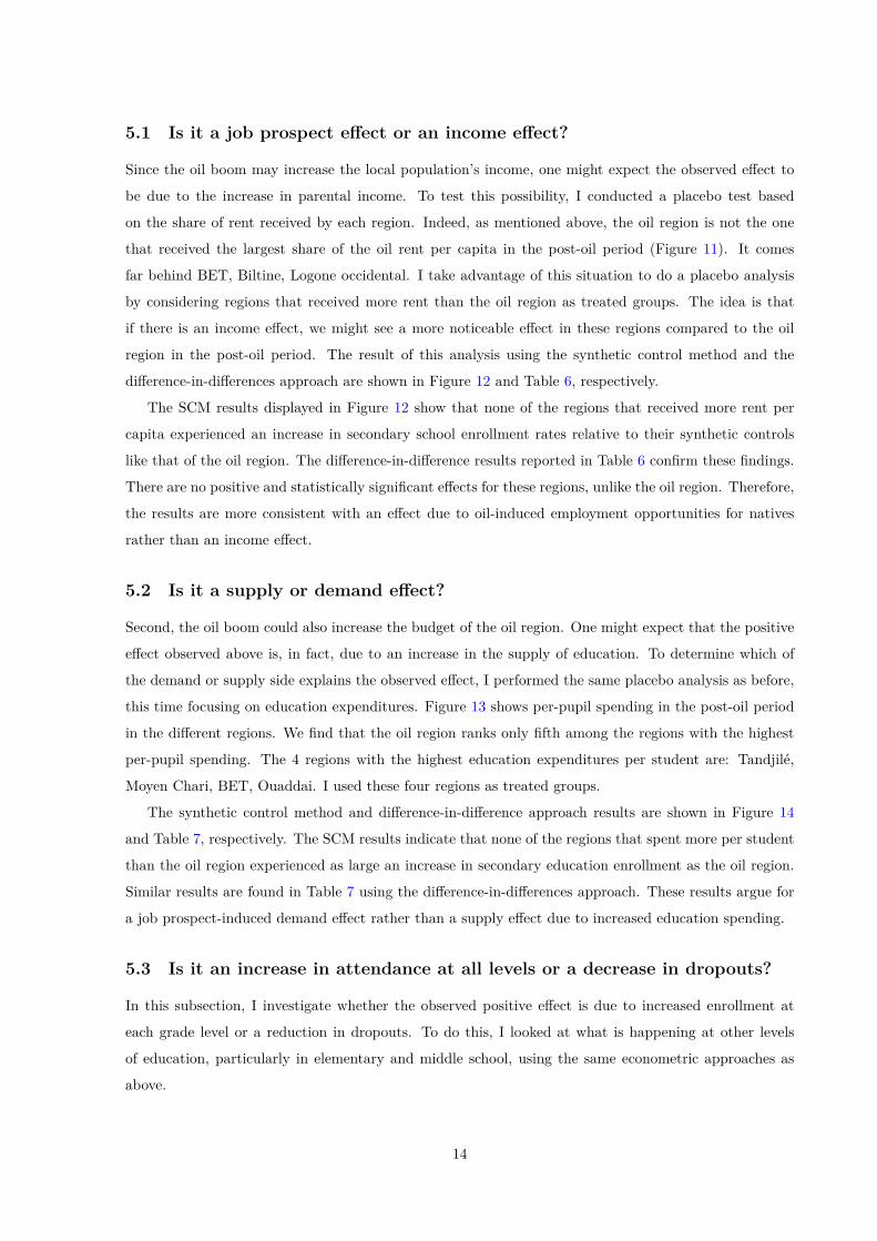
5.1 Is it a job prospect effect or an income effect?
Since the oil boom may increase the local population’s income, one might expect the observed effect to
be due to the increase in parental income. To test this possibility, I conducted a placebo test based
on the share of rent received by each region. Indeed, as mentioned above, the oil region is not the one
that received the largest share of the oil rent per capita in the post-oil period (Figure 11). It comes
far behind BET, Biltine, Logone occidental. I take advantage of this situation to do a placebo analysis
by considering regions that received more rent than the oil region as treated groups. The idea is that
if there is an income effect, we might see a more noticeable effect in these regions compared to the oil
region in the post-oil period. The result of this analysis using the synthetic control method and the
difference-in-differences approach are shown in Figure 12 and Table 6, respectively.
The SCM results displayed in Figure 12 show that none of the regions that received more rent per
capita experienced an increase in secondary school enrollment rates relative to their synthetic controls
like that of the oil region. The difference-in-difference results reported in Table 6 confirm these findings.
There are no positive and statistically significant effects for these regions, unlike the oil region. Therefore,
the results are more consistent with an effect due to oil-induced employment opportunities for natives
rather than an income effect.
5.2 Is it a supply or demand effect?
Second, the oil boom could also increase the budget of the oil region. One might expect that the positive
effect observed above is, in fact, due to an increase in the supply of education. To determine which of
the demand or supply side explains the observed effect, I performed the same placebo analysis as before,
this time focusing on education expenditures. Figure 13 shows per-pupil spending in the post-oil period
in the different regions. We find that the oil region ranks only fifth among the regions with the highest
per-pupil spending. The 4 regions with the highest education expenditures per student are: Tandjilé,
Moyen Chari, BET, Ouaddai. I used these four regions as treated groups.
The synthetic control method and difference-in-difference approach results are shown in Figure 14
and Table 7, respectively. The SCM results indicate that none of the regions that spent more per student
than the oil region experienced as large an increase in secondary education enrollment as the oil region.
Similar results are found in Table 7 using the difference-in-differences approach. These results argue for
a job prospect-induced demand effect rather than a supply effect due to increased education spending.
5.3 Is it an increase in attendance at all levels or a decrease in dropouts?
In this subsection, I investigate whether the observed positive effect is due to increased enrollment at
each grade level or a reduction in dropouts. To do this, I looked at what is happening at other levels
of education, particularly in elementary and middle school, using the same econometric approaches as
above.
14

First of all, we see in Figure 15 that the primary and middle schooling rate is initially higher in the
oil region than in the rest of Chad. In Figure 16, I construct a synthetic oil region as in subsection
4.1 using a number of pre-treatment predictors. The predictor variables are the same as those used for
secondary education, except for the proportion of children aged 6 to 17 and the primary and middle
school enrollment rate before treatment considered in this subsection. We particularly note that the
evolution of the net primary and intermediate schooling rate before the oil is the same in the oil region
and its synthetic control.
In Figure 17, I present the difference in results between the region’s oil and its synthetic control over
the entire period considered. This graph clearly shows that the difference is almost zero even after oil.
Oil-induced employment opportunities for natives do not appear to have positively affected primary and
secondary school enrollment. Placebos tests confirm this absence of a positive and statistically significant
effect. Indeed, in Figure 18, we observe that compared to the non-oil regions used as placebos, the oil
region does not record a significant increase as in the previous section. Furthermore, Table 8 shows
that the oil region is ranked in sixth place in post-pre-oil MSPE ratios. The use of survey data or the
difference-in-differences method does not change the results, as shown in Tables 9 and 12. Regardless
of the specification chosen, these two tables show that the oil-induced employment opportunities and
pro-native policies had no statistically significant effect on primary and middle education.
These results are consistent with the lack of a positive effect noted above. The fact that there is no
effect on elementary and middle school enrollment indicates that the effect observed at the secondary
school level is less likely to be due to increased parental income.
5.4 Migration issues
The other main concern that could challenge the findings is migration. Indeed, if many people migrate
to the oil region to benefit from the oil boom, it may be that the observed effect is due to this migratory
movement and not to a decrease in school dropout, as indicated in the previous subsection. I check this
concern by looking at the evolution of the immigrant population’s share before and after the oil boom.
In figure 19, we successively present the evolution of the total population, the number of immigrants, and
what these immigrants represent in the total population of the oil region. Regarding the total population,
we see that it almost doubled between 1993 and 2009, going from 376,875 to 750,649. At the same time,
the number of immigrants to the region has tripled, from 17,414 in 1993 to 58,856 in 2009. Relative to
the total population, the share of immigrants increased from 5% in 1993 to 8% in 2009. However, most of
this increase occurred before exploitation started in 2004. The share of migrants in the total population
increased by only 1% between 2004 and 2009. Unfortunately, in the regressions, the data do not precisely
identify the immigrant population, but this low increase in the share of immigrants between 2004 and
2009 suggests that no mass migration could significantly affect the results. Moreover, as we will see in
the next section, controlling or not by the household characteristics does not change the results.
15

6 Robustness Checks
Although the placebo tests and the difference-in-differences approach show the robustness of our results,
the small sample size may pose a problem of statistical power. To solve this problem, I re-estimate the
effect of the treatment on schooling using nationally representative survey data. More specifically, I use
the Demographic and Health Surveys (1996, 2004), the Multiple Indicator Cluster Surveys (2000, 2009),
and the Survey on Household Living Conditions and Poverty in Chad (2010). The sampling frame for all
these surveys comprises the enumeration areas (ZD) of the central census office of the National Institute
of Statistics and Economic and Demographic Studies (INSEED) in Chad. The main variables used in
this section are presented in Table 10. This table shows no fundamental difference between the oil region
and the rest of Chad in terms of main household characteristics (head, school-aged children, etc.).
Using the data from this survey, I then applied the difference-in-differences approach to estimate the
effect oil-induced employment opportunities for natives on secondary schooling in the oil region. These
estimates are presented in the Table 11. In the first column, I estimated the effect without any control
variable. In the second, I control for household and head of household characteristics. These control
variables are household size, sex, age, the household’s head level of education, an indicator variable for
the head of household, the share of dependents (child and eldest) in the household, and the sex of the
child. In column 3, I add another variable to these controls, which indicates whether the household
belongs to the first, second, third, fourth, and fifth wealth quintiles. Standard errors are clustered at the
regional level.
First of all, it should be noted that the graph 20 presented in the appendix shows that the parallel trend
assumption necessary to estimate a causal effect using the difference-in-differences method is respected.
Then, the positive and significant effect of the treatment on secondary education in the oil region presented
in the last section remains unchanged. Although the magnitude of the effect is slightly smaller than shown
above, the interaction term shows a positive and significant effect of oil-induced employment opportunities
for natives on secondary education. This finding is robust to all specifications. Therefore, the sample
size issue mentioned above does not appear to alter our results drastically.
7 Concluding Remarks
This article analyzed the effect of oil-induced employment opportunities for natives on secondary school
enrollment decisions in Chad’s oil-rich region. First, I used administrative data and the synthetic control
method to create a synthetic oil region, indicating what would happen in the oil region without these
possibilities. I then compared the results for the synthetic oil region with the actual results for the oil
region. I have found a positive and statistically significant effect of oil-induced employment opportunities
for natives on the secondary school enrollment rate in the oil region. This rate increased by around 5%
in the oil region compared to its synthetic control. Next, I used the difference-in-differences method to
compare the evolution of secondary school enrollment in the oil region before and after the oil boom with
16

that of the control regions over the same period. This second analysis confirms those obtained by the
synthetic control method previously. Specifically, I find that the treatment increased secondary school
enrollment by 6% in the oil region. I obtained similar results when I used nationally representative survey
data rather than administrative data.
In terms of mechanism, the results first show that the observed effect is not an income effect since
none of the regions that received more rent than the oil region experienced an increase in enrollment
equivalent to that of the oil region. Second, I show that the observed increase in enrollment results from
an increase in demand for education rather than an increase in education spending. Indeed, no region
that spent the most per student experienced a similar increase as the oil region. These results confirm the
role of labor market incentives on schooling decisions. Furthermore, I investigated whether this result was
due to a decrease in the dropout rate in the oil region or increased enrollment at all levels of education.
When I analyzed primary and middle school enrollment, I found that the observed effect was more due
to a decrease in dropouts than an overall increase in enrollment at all levels.
This paper raises important questions about human capital investment in developing countries and
has significant policy implications. First, I find that employment prospects are vital determinants of
educational decision-making in Chad. Therefore, programs to increase human capital should incorporate
returns to education into their design. Second, the results suggest that demand appears to be a limiting
factor in the level of education in Chad. This demand effect explains Chad’s low secondary school
attendance and higher early dropout rate despite massive investments in education. Hence, improving
work prospects may be an effective way to combat school dropout in this country. Furthermore, to
increase human capital in Chad and create decent jobs, the authorities should implement awareness
campaigns for parents and children on labor market opportunities and the importance of education for
professional success.
17
ReferencesAbadie, A., Diamond, A. & Hainmueller, J. (2010), ‘Synthetic control methods for comparative case studies: Estimating
the effect of california’s tobacco control program’, Journal of the American statistical Association 105(490), 493–505.
Abadie, A. & Gardeazabal, J. (2003), ‘The economic costs of conflict: A case study of the basque country’, American
economic review 93(1), 113–132.
Akresh, R., Halim, D. & Kleemans, M. (2018), Long-term and intergenerational effects of education: Evidence from school
construction in indonesia, Technical report, National Bureau of Economic Research.
Athey, S. & Imbens, G. W. (2017), ‘The state of applied econometrics: Causality and policy evaluation’, Journal of Economic
Perspectives 31(2), 3–32.
Attanasio, O. & Kaufmann, K. (2014), ‘Education choices and returns to schooling: Intrahousehold decision making, gender
and subjective expectations’, Journal of Development Economics 109, 203–216.
Becker, G. S. (1964), ‘A theoretical and empirical analysis, with special reference to education’.
Cascio, E. U. & Narayan, A. (2015), Who needs a fracking education? the educational response to low-skill biased techno-
logical change, Technical report, National Bureau of Economic Research.
Caselli, F. & Michaels, G. (2013), ‘Do oil windfalls improve living standards? evidence from brazil’, American Economic
Journal: Applied Economics 5(1), 208–38.
Duflo, E. (2001), ‘Schooling and labor market consequences of school construction in indonesia: Evidence from an unusual
policy experiment’, American economic review 91(4), 795–813.
EDS-MICS (2014), ‘Enquête démographique et de santé et à indicateurs multiples au tchad (eds-mics) 2014-2015.’, pp. 655
p., annexes.
Emery, J. H., Ferrer, A. & Green, D. (2012), ‘Long-term consequences of natural resource booms for human capital
accumulation’, ILR Review 65(3), 708–734.
Goodman, S., BenYishay, A., Lv, Z. & Runfola, D. (2019), ‘Geoquery: Integrating hpc systems and public web-based
geospatial data tools’, Computers & geosciences 122, 103–112.
Gylfason, T. (2001), ‘Natural resources, education, and economic development’, European economic review 45(4-6), 847–859.
Henderson, J. V., Storeygard, A. & Weil, D. N. (2012), ‘Measuring economic growth from outer space’, American economic
review 102(2), 994–1028.
INSEED (2013), ‘Profil de pauvreté au tchad en 2011’, Tchad: Institut National de la Statistique et des Etudes Economiques
et Démographiques. .
James, A. (2015), Is education really underfunded in resource-rich economies? evidence from a panel of us states, Technical
report, University of Alaska Anchorage, Department of Economics.
Jensen, R. (2010), ‘The (perceived) returns to education and the demand for schooling’, The Quarterly Journal of Economics
125(2), 515–548.
Kaufmann, K. M. (2014), ‘Understanding the income gradient in college attendance in mexico: The role of heterogeneity
in expected returns’, Quantitative Economics 5(3), 583–630.
Keola, S., Andersson, M. & Hall, O. (2015), ‘Monitoring economic development from space: using nighttime light and land
cover data to measure economic growth’, World Development 66, 322–334.
18

Kojucharov, N. (2007), ‘Poverty, petroleum & policy intervention: Lessons from the chad-cameroon pipeline’, Review of
African Political Economy 34(113), 477–496.
Kumar, A. (2017), ‘Impact of oil booms and busts on human capital investment in the usa’, Empirical Economics
52(3), 1089–1114.
Lucas, R. E. (1998), ‘On the mechanics of economic development’, Econometric Society Monographs 29, 61–70.
Mabali, A. & Mantobaye, M. (2015), Oil and regional development in chad: Impact assessment of doba oil project on the
poverty in host region, Technical report, HAL.
Mankiw, N. G., Romer, D. & Weil, D. N. (1992), ‘A contribution to the empirics of economic growth’, The quarterly journal
of economics 107(2), 407–437.
Manski, C. F., Wise, D. A. & Wise, D. A. (1983), College choice in America, Harvard University Press.
Nguyen, T. (2008), ‘Information, role models and perceived returns to education: Experimental evidence from madagascar’,
Unpublished manuscript 6.
Pinkovskiy, M. & Sala-i Martin, X. (2016a), ‘Lights, camera… income! illuminating the national accounts-household surveys
debate’, The Quarterly Journal of Economics 131(2), 579–631.
Pinkovskiy, M. & Sala-i Martin, X. (2016b), Newer need not be better: evaluating the penn world tables and the world
development indicators using nighttime lights, Technical report, National Bureau of Economic Research.
Raimi, D. & Newell, R. G. (2014), ‘Shale public finance’, Durham, NC: Duke University Energy Initiative .
Rickman, D. S., Wang, H. & Winters, J. V. (2017), ‘Is shale development drilling holes in the human capital pipeline?’,
Energy Economics 62, 283–290.
Unesco (2015), ‘Tchad : rapport d’état sur le système éducatif national : éléments d’analyse pour une refondation de l’école’,
pp. 213 p., annexes.
Unesco (2016), ‘Global education monitoring report summary 2016: education for people and planet: creating sustainable
futures for all’.
Unesco (2018), ‘One in five children, adolescents and youth is out of school’.
Weber, J. G., Burnett, J. W. & Xiarchos, I. M. (2016), ‘Broadening benefits from natural resource extraction: Housing
values and taxation of natural gas wells as property’, Journal of Policy Analysis and Management 35(3), 587–614.
Zuo, N., Schieffer, J. & Buck, S. (2019), ‘The effect of the oil and gas boom on schooling decisions in the us’, Resource and
Energy Economics 55, 1–23.
19

Figure 1: Administrative map (region) of Chad
20

Figure 2: Oil revenues collected by the oil region from 2004 to 2012
21

Figure 3: Investments by sector in the oil region over the period 2005-2012
22

Figure 4: Trends in the net secondary school enrollment rate : oil region vs rest of Chad
23

Table 1: Descriptive statistics of predictors
Mean SdEnrolment (1993) 3.08 3.71Enrolment (1996) 6.61 5.58Enrolment (2000) 6.75 5.54Enrolment (2002) 10.8 11.7Enrolment (2004) 10.1 8.86Share of 15-64(1993) 35.8 2.98Share of 15-64(1996) 34.0 2.70Share of 15-64(2000) 30.9 3.14Share of 15-64(2002) 36.0 3.76Share of 15-64(2004) 32.9 3.21Urbanisation (1993) 2.79 0.75Urbanisation (1996) 3.34 0.54Urbanisation (2000) 3.84 0.36Urbanisation (2002) 3.56 0.45Urbanisation (2004) 3.56 0.45Precipitation (1993) 3.48 0.97Precipitation (1996) 3.60 1.05Precipitation (2000) 3.71 0.74Precipitation (2002) 3.57 0.70Precipitation (2004) 3.68 0.88Cropland (1993) 10.4 1.70Cropland (1996) 10.5 1.69Cropland (2000) 10.5 1.69Cropland (2002) 10.5 1.69Cropland (2004) 10.5 1.69Nighttime lights (1993) 0.080 0.19Nighttime lights (1996) 0.073 0.14Nighttime lights (2000) 0.057 0.10Nighttime lights (2002) 0.055 0.096Nighttime lights (2004) 0.088 0.12Private tuition per pupil(2004) 1409 1834Education expenditure per pupil(2004) 12621 19891
N 75
Note: Share of 15-64 is the percentage of the population aged 15 to 64. Urbanization is the logarithm of the share ofthe urban population in the total population. Cropland represents the logarithm of rain-fed cropland area. Nighttimelights are Nighttime lights per density. Education expenditure per pupil are averaged for the 1993–2004 period.
24

Table 2: Balancing table of predictors of the net secondary school enrollment rate
(1) (2)Oil Region Average of
Real Synthetic control states
Enrolment rate(1993) 2.74 3.06 3.11Enrolment rate(1996) 6.44 6.48 6.63Enrolment rate(2000) 6.18 6.62 6.79Enrolment rate(2002) 9.81 9.77 10.82Enrolment rate(2004) 10.12 10.09 10.1Share of 15-64(1993) 35.56 36.43 35.87Share of 15-64(1996) 35.32 34.89 33.90Share of 15-64(2000) 32.26 31.30 30.85Share of 15-64(2002) 34.76 35.56 36.07Share of 15-64(2004) 33.93 31.58 32.85Urbanisation(1993)) 2.31 2.45 2.83Urbanisation(1996) 3.02 3.12 3.36Urbanisation(2000) 3.69 3.66 3.85Urbanisation(2002) 3.52 3.52 3.56Urbanisation(2004) 3.52 3.52 3.56Precipitation(1993) 4.33 3.28 3.41Precipitation(1996) 4.55 3.39 3.53Precipitation(2000) 4.49 3.59 3.65Precipitation(2002) 4.28 3.42 3.52Precipitation(2004) 4.52 3.47 3.62Cropland(1993) 9.47 9.66 10.51Cropland(1996) 9.62 9.68 10.53Cropland(2000) 9.65 9.71 10.56Cropland(2002) 9.66 9.71 10.56Cropland(2004) 9.67 9.72 10.57Nighttime lights(1993) 0.09 0.09 0.08Nighttime lights(1996) 0.11 0.07 0.07Nighttime lights(2000) 0.08 0.06 0.05Nighttime lights(2002) 0.07 0.08 0.05Nighttime lights(2004) 0.13 0.12 0.09Private tuition per pupil (2004) 1553 1555 1399Public expenditure per pupil(2004) 14943 14980 12455
Note: Share of 15-64 is the percentage of the population aged 15 to 64. Urbanization is the logarithm of the share ofthe urban population in the total population. Cropland represents the logarithm of rain-fed cropland area. Nighttimelights are Nighttime lights per density. Education expenditure per pupil are averaged for the 1993–2004 period.
25

Figure 5: Oil region net secondary school enrollment rate vs Synthetic oil region
26

Figure 6: Gap between actual oil region vs Synthetic oil region in net secondary school enrollment rate
27

Table 3: Region weights in the synthetic Oil Region
Region Weight
Batha 0
BET 0.07
Biltine 0.17
Chari-Baguirmi 0
Guéra 0
Kanem 0
Lac 0.29
Logone Occidental 0
Mayo-Kebbi 0
Moyen-Chari 0.10
Ouaddaï 0
Salamat 0
Tandjilé 0.28
N’Djamena 0.09
Treated Unit : Oil region(Logone Oriental) 1
28

Figure 7: Oil Region and Placebo distribution
29

Figure 8: Ratio of post-oil MSPE and pre-oil MSPE: Oil region and control regions.
30

Table 4: Synthetic control results
Variables Value
Panel A : Model fit pre-intervention
RMPSE 0.25
APE-to-mean ratio 3.54%
Panel B : Placebo test
RMSPE ratio 22.72
P-value∗ 0.06
Panel C : Synthetic control ATT
ATT 4.78*
Treatment rank 1
*** p<0.01, ** p<0.05, * p<0.1. ATT : difference in the mean differences, between enrollment rate in oil region andthat of the synthetic control, in the pre-treatment period from that in the post-treatment period. APE-to-mean ratioindicates the average pre-oil prediction error divided by the average pre-oil outcome value. P-value∗ calculated basedon placebo tests
31
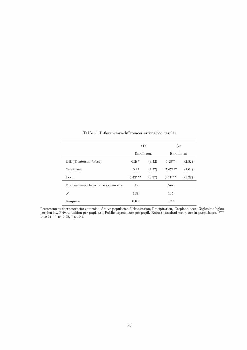
Table 5: Difference-in-differences estimation results
(1) (2)
Enrollment Enrollment
DID(Treatement*Post) 6.28* (3.42) 6.28** (2.82)
Treatment -0.42 (1.57) -7.67*** (2.04)
Post 6.43*** (2.37) 6.43*** (1.27)
Pretreatment characteristics controls No Yes
N 165 165
R-square 0.05 0.77
Pretreatment characteristics controls : Active population Urbanisation, Precipitation, Cropland area, Nighttime lightsper density, Private tuition per pupil and Public expenditure per pupil. Robust standard errors are in parentheses. ***p<0.01, ** p<0.05, * p<0.1.
32

Figure 9: Estimated effect of treatment on the net secondary school enrollment rate using difference-in-differences
33

Figure 10: Share of oil revenues received and demographic weight by region
Figure 11: The ratio of oil revenues received in proportion to the demographic weight by region
34

Figure 12: Oil region vs Regions with the most oil revenue per capita
Table 6: Difference-in-difference estimation results for major rent recipients
(1) (2) (3)
BET Biltine Logone occidental
Coef. se Coef. se Coef. se
DID(Treatement*Post) -6.97 (9.37) -7.16 (9.40) 6.67 (9.38)
Treatment -6.23 (6.92) -5.07 (6.94) 6.41 (6.92)
Post 7.31*** (2.42) 7.32*** (2.43) 6.40*** (2.42)
R-square 0.08 0.07 0.08
*** p<0.01, ** p<0.05, * p<0.1
35

Figure 13: Post-oil public expenditure per student
36

Figure 14: Oil region vs Regions that spent the most on education per student
Table 7: Difference-in-difference estimation results : Regions that spent the most on education per student
(1) (2) (3) (4)
BET Moyen Chari Ouaddai Tandjilé
Coef. se Coef. se Coef. se Coef. se
DID(Treatement*Post) -6.97 (9.37) -1.28 (9.51) -7.76 (9.44) 1.45 (9.52)
Treatment -6.23 (6.92) 3.32 (7.03) -2.56 (6.97) -0.51 (7.03)
Post 7.31*** (2.42) 6.93*** (2.46) 7.36*** (2.44) 6.75*** (2.46)
R-square 0.08 0.05 0.07 0.05
*** p<0.01, ** p<0.05, * p<0.1
37

Figure 15: Trends in the net primary and middle school enrollment rate : oil region vs rest of Chad
38

Figure 16: Oil region net primary and middle school enrollment rate vs Synthetic oil region
39

Figure 17: Gap between actual oil region vs Synthetic oil region in net primary and middle schoolenrollment rate
40

Figure 18: Oil Region and Placebo distribution
41

Table 8: Synthetic control results : Effect of oil on net primary and middle school enrollment rate
Variables Value
Panel A : Model fit pre-intervention
RMPSE 0.27
APE-to-mean ratio 4.86%
Panel B : Placebo test
RMSPE ratio 1.96
p-value∗ : 0.40
Panel C : Synthetic control ATT
ATT 0.011
Treatment rank 6
*** p<0.01, ** p<0.05, * p<0.1. ATT : difference in the mean differences, between enrollment rate in oil region andthat of the synthetic control, in the pre-treatment period from that in the post-treatment period. APE-to-mean ratioindicates the average pre-oil prediction error divided by the average pre-oil outcome value. p-value∗ calculated based onplacebo tests.
42

Table 9: Difference-in-differences estimation results : Effect of oil on net primary and middle schoolenrollment rate
(1) (2)
Enrollment Enrollment
DID(Treatement*Post) 2.25 (5.35) 2.25 (4.89)
Treatment 13.28*** (4.73) 1.27 (5.25)
Post 10.17*** (2.88) 10.17*** (1.63)
Pretreatment characteristics controls No Yes
N 165 165
R-square 0.12 0.73
*** p<0.01, ** p<0.05, * p<0.1. Pre-treatment characteristics controls are the share of population under 15, Urbani-sation, Precipitation, Cropland area, Nighttime lights per density, Private tuition per pupil and Public expenditure perpupil. Standard errors in parentheses are obtained clustering observations at region level.
43

Figure 19: Evolution of the total population, the number of immigrants and the proportion of immigrantsin the oil region
44

Table 10: Descriptive statistics of the main variables in the survey data
(1) (2)
Oil Region Rest of Chad
Mean. Sd Mean. Sd
Enrollment rate 14.96 (35.69) 15.30 (36.00)
household size 7.95 (4.52) 7.85 (5.05)
Age of HH 41.68 (14.67) 44.71 (14.91)
Sex of HH 0.84 (0.37) 0.82 (0.38)
Child of HH 0.39 (0.49) 0.48 (0.50)
Non educated HH 0.37 (0.48) 0.56 (0.50)
Share of women 0.31 (0.19) 0.34 (0.21)
Share of elder 0.02 (0.06) 0.02 (0.07)
Share of child < 6 0.16 (0.15) 0.13 (0.14)
Sex of child 0.49 (0.50) 0.49 (0.50)
Lowest 20% 0.14 (0.35) 0.12 (0.32)
Second 20% 0.20 (0.40) 0.15 (0.36)
Third 20% 0.20 (0.40) 0.17 (0.37)
Fourth 20% 0.23 (0.42) 0.22 (0.42)
Top 20% 0.24 (0.43) 0.34 (0.48)
N 1441 28301
Source : Authors from DHS, MICS and ECOSIT data. *** p<0.01, ** p<0.05, * p<0.1.
45

Figure 20: Parallel trend assumption
46

Table 11: Difference-in-differences estimation results using survey Data
(1) (2) (3)
Enrolment Enrolment Enrolment
DID(Post*Treatement) 3.36* (2.03) 2.87* (1.61) 3.19* (1.64)
Treatement -1.69 (1.38) -4.05 (2.77) -2.20 (1.46)
Post 13.54*** (0.44) 13.92*** (1.67) 14.16*** (1.63)
Household characteristics No Yes Yes
Wealth controls No No Yes
N 26853 26552 26552
R-square 0.04 0.12 0.14
Source : Authors from DHS, MICS and ECOSIT data. Household and head of the household characteristics are thesize of the household, sex, age, education of the head of the household, a dummy for the child of the household, theshare of dependents (child and elder) in the household and the sex of the child. Wealth controls are dummy variables,which indicate whether the household is in the first, second, third, fourth and fifth wealth quintiles. Standard errors inparentheses are obtained clustering observations at region level. *** p<0.01, ** p<0.05, * p<0.1.
47

Table 12: Difference-in-differences estimation results using survey Data : Effect of oil on net primary andmiddle school enrollment rate
(1) (2) (3)
Enrolment Enrolment Enrolment
DID(Post*Treatement) 2.32 (1.75) 1.47 (3.25) 0.49 (2.14)
Treatement 14.14*** (1.26) 5.61 (4.33) 10.23*** (2.76)
Post 14.21*** (0.40) 12.59*** (3.61) 14.86*** (2.37)
Household characteristics No Yes Yes
Wealth controls No No Yes
N 65257 65226 65226
R-square 0.02 0.17 0.20
Source : Authors from DHS, MICS and ECOSIT data. Standard errors in parentheses are obtained clustering observa-tions at region level. *** p<0.01, ** p<0.05, * p<0.1.
48