AD-A258 716

PL-TR-92-2209

SIMULATION AND CALCULATION OF THE APEXATTITUDE

DTICW. J. McNeil _ E VI 2 1992 1

CRadex, Inc.Three Preston CourtBedford, MA 01730

29 July 1992

Scientific Report No. 11

Approved for public release; distribution unlimited 92-29309

PHILLIPS LABORATORYDirectorate of GeophysicsAIR FORCE MATERIEL COMMANDHANSCOM AIR FORCE BASE, MA 01731-5000

"This technical report has been reviewed and is approved for publication"

EDWARD C. ROBINSONContract ManagerData Analysis Division

ROBE!RT E. M~cINENEy•,-D •btor

Data Analysis Division

This report has been reviewed by the ESD Public Affairs Office (PA) and isreleasable to the National Technical Information Service (NTIS).

Qualified requestors may obtain additional copies from the Defense TechnicalInformation Center. All others should apply to the National TechnicalInformation Service.

If your address has changed, or if you wish to be removed from the mailinglist, or if the addressee is no longer employed by your organization, pleasenotify GL/IMA, Hanscom AFB, MA 01731. This will assist us in maintaining acurrent mailing list.

Do not return copies of this report unless contractual obligations ornotices on a specific document requires that it be returned.

Form 4ppro ' r "IREPORT DOCUMENTATION PAGE UMB No c4 CF8

S a and.....~-, Calc-ulatio o.-e 'e 10E A d P 62101F'CA

1. AGENCY USE ONLY ke a .EPORT DATE 3. REPORT TYPE AND DATES COVERED

1 29 July 1992 Scientific Report No. 11

4. TITLE AND SUBTITLE 5. FUNDING NUMBERS

Simulation and Calculation of the APEX Attitude PE 62101FPR 7659 TA 05 WU AB

6. AUTHOR(S)

Contract F 162X89-C-0068

W. J. McNeil

7. PERFORMING ORG-ANiZ:TION NAME(S) AND ADORESS(ES) 8. PERFORMING ORGANIZATIONREPORT NuMBFR

RADEX, Inc.

Three Preston CourtBedford, MA 01730 RXR-92072

9. ZNSORINC ';C?,TCRNG A•GENCY NAME(S) AND ADDRESS(ES) 10. SPONSORINGMONITOR!NG

Phillips Laboratory AGENCY REPORT NUMBER

Hanscom AFB, MA 01731-5000

Contract Manager: Edward C. Robinson/GPD PL-TR-92-2209

2z. :':STR:E'.UT CN AA\' A E ;LTY STATEMENT 12b. DISTFiEUTION CODE

Approved for Public ReleaseDistribution Unlimited

1 ~':~RCT ' .

A simulation of the APEX attitude is carried out for purposes of development andtesting of attitude computation algorithms and for assessment of the accuracy of post-flight attitude determination.It is found that reasonably tractable algorithms give adequate accuracy for determination of attitude control in thevehicle. Sun normal angle will be known to a high precision during sunlit operations. The roll axis in sunlight andthe three axes during eclipse will be somewhat less precise, depending mainly on the degree of magneticcontamination. However, it is estimated that these quantities will be of sufficient accuracy as well.

•. S CT i"'11 115. NUMBER CIF PAGESAttitude SIMulation, Attitude determination, APEX attitude 54

16. PRICE CODE

17. SECURITY CLASSFICALCN 8 SECURITY CLASSIFICATION 19 SECURITY CLASSIFICATION 20. LIMITATION OF ABSTRACTdF FEP06T. OF THIS PAGE OFC ASTRACT

nclassi•ied Unclassified Unclassified Unlimited

:*CB ".2

TABLE OF CONTENTS

Section Page

1.0 INTRODUCTION ....................................................... 1

2.0 DEFINITION OF THE ATTITUDE .......................................... 22.1 CONVERSION TO INERTIAL COORDINATES ......................... 22.2 CONVERSION FROM INERTIAL COORDINATES ...................... 6

3.0 MODELING THE ATTITUDE .............................................. 73.1 EPHEMERIS MODELING .......................................... 73.2 MODELING ENVIRONMENTAL TORQUES ........................... 83.3 MODELING CONTROL LAWS ...................................... 93.4 INCLUDING MAGNETOMETER EFFECTS ........................... 123.5 ECLIPSE CONTROL LAWS ........................................ 133.6 EQUATIONS OF MOTION ........................................ 133.7 SIMULATION RESULTS .......................................... 143.8 SIMULATION OF INSTRUMENTS .................................. 21

4.0 ATTITUDE SOLUTION ALGORITHMS ..................................... 224.1 MAGNETOMETER CALIBRATION ................................. 224.2 ATTITUDE SOLUTIONS IN SUNLIGHT ............................. 234.3 ATTITUDE SOLUTIONS IN ECLIPSE ............................... 32

5.0 EVALUATION OF ON-BOARD ATTITUDE ................................... 41

6.0 CO NCLUSIO N ........................................................ 43

REFERENCES ........................................................... 45

APPENDIX. STATE VECTORS .............................................. A-1

//

! AvXLSObflOtd C~e

Diessr'eles Fo

ii.. Speci ndlorIDist iSpeci~al

W-\

LIST OF FIGURES

Figur Page

1. Pitch, yaw and roll angles defining the APEX Attitude ............................. 3

2. Two possible configurations satisfying the nominal attitude requirements ................ 4

3. Typical aerodynamic and gravity gradient torques for APEX ........................ 10

4. Typical pitch and yaw angles during sunlit operation .............................. 15

5. Values of roll axis attitude with low and high frequency induced fields ................. 16

6. Roll axis attitude with various static induced fields ................................. 18

7. Torque rod com m ands .................................................... 19

8. Pitch and yaw angles for orbits with eclipses .................................... 20

9. Results of magnetometer calibration with Bi=200 and Br= 120 nT .................... 24

10. Same as Figure 9 but with Bi=500 nT ........................................ 25

11. Pitch and yaw angles calculated during sunlit operation ........................... 27

12. Roll axis, actual and calculated with and without calibration ........................ 29

13. Calibrated roll error in sunlight ............................................. 30

14. Errors in roll arising from timing & ephemeris errors ............................ 31

15. Pitch, yaw and roll during eclipse ........................................... 33

16. Best fit solution with constant attitude for data in Figure 15 ........................ 36

17. Attitude and solution for Eclipse 2 of Case 10 .................................. 37

18. Attitude and solution for a non-nominal case ................................... 39

19. Attitude and constant solution for no control during eclipse ........................ 40

20. Same as Figure 19 but with linear term in 4 .................................... 42

21. Case 9 Eclipse 2 solution with fixed derivatives ................................. 44

iv

LIST OF TABLES

Table Page

1. Control Law Coefficients .................................................. 11

V

ACKNOWLEDGEMENTS

We greatly appreciate the efforts of Al Griffin, PIJGPD, DennisDelorey, Boston College, who have assisted in the ground work necessaryfor the understanding of the attitude requirements of this mission and ofthe specifics of the attitude instruments. Rick Barnison, of OrbitalSciences Corp., has been most helpful in regards to the attitude controlsystem and the instruments. The orbit propagator used to generate testel ments was provided by Johnny Kwok of JPL.

vi

1.0 INTRODUCTION

In the design, development and testing of attitude determination and processing algorithms, itis necessary to perform at least a rudimentary simulation of the satellite orbit and data from theattitude instruments. This is especially true for actively controlled satellites, since the attitudecharacteristics depend on the interplay between the environmental torques and controlmechanisms of the satellite. In order to assess the feasibility of computational techniques,realistic data must be generated. Sirmulation is also necessary for the generation of software testdata and it is valuable in that it gives one a sense of the type of behavior to expect, althoughperhaps not in a truly precise manner, before launch. This often dramatically decreases thestart-up time for data processing. This report details the modeling carried out for the AdvancedPhotovoltaic and Electronic Experiment (APEX) satellite (P90-1). It describes the algorithmsselected for the post-flight Orbital Data Processing System for calibration of the magnetometerand for attitude computation. As a by-product, several interesting features that may be presentin the APEX attitude behavior are noted.

The APEX satellite suppor!g three experiments; the Photovoltaic Array Space Power PlusDiagnostics (PASP-Plus) experiment, the Cosmic Ray Upset Experiment/Cosmic RayEnvironment and Dosimeter Experiment (CRUX/CREDO), and the Ferroelectric MemoryExperiment (FERRO). Attitude control requirements are strictest during sunlit operation, whenthe sun must be normal to the solar arrays to within one-half degree. This requires thespacecraft x-axis to be collinear with the sun direction to this precision. A second, less preciserequirement is that the dosimeter (spacecraft y-axis) lie in the ecliptic plane to within 5'. Thereare no set requirements for attitude knowledge, however, knowledge must be sufficient to assessthe level of control. For the APEX satellite, assessment of the degree of attitude control is theprimary purpose of post-flight attitude computation.

The attitude determination instruments aboard the satellite consist of a two-axis sun sensor,which measures the sun normal vector directly, and a magnetometer, which can be used tocalculate the roll angle during sunlit operation and three-axis attitude in eclipse. Knowledge ofthe x-axis relative to the sun is thus readily available when the solar panels are illuminated. Thesecondary requirement for roll axis attitude in sunlight and three-axis attitude in eclipse must beevaluated from magnetometer data alone. Such calculations are unvaryingly quite sensitive tocalibration errors and to spacecraft induced fields, so that calibration of the instrument arndevaluation of the spacecraft cleanliness become synonymous with attitude determination.

The purpose of this work is to investigate the dynamics of the satellite under 'nominal'conditions, to define and assess algorithms for calibration of the magnetometer and for attitudecalculation and ultimately to demonstrate that attitude can be calculated with sufficient accuracyfor determination of the degree of attitude control. It is not the subject of this work to dcterminewhether such control will be possible in flight, however, we would like to be reasonably surethat the attitude is calculated properly should non-nominal situations arise. In the next section,the attitude is defined. Following this, we discuss the modeling of the APEX ephemeris,environmental torques and control laws. Finally, we demonstrate the algorithms chosen for

I

magnetometer calibration and for attitude calculation. In the course of this work, we are ableto arrive at some rough estimates for the accuracy of the calculated attitude.

2.0 DEFINITION OF THE ATTITUDE

Generally speaking, it is possible to define the spacecraft .ttitude in several ways, so long as theprocess of computation and utilization of the attitude solution are based on the same definition.However, because the APEX data stream contains an on-board attitude solution as well as rawsensor data, it is necessary to adopt the same definition for post-flight determination as is usedin the on-board solution.

The APEX attitude is defined by three angles, the values of which are simultaneously zero whenthe spacecraft is in its nominal attitude. This nominal attitude consists of the spacecraft x-axispointed directly toward the sun and the spacecraft y-axis resting in the earth's ecliptic plane.These three angles are further defined by rotations about the three spacecraft axes. These angleswill be called Ox, 0y and 0z in what follows. Figure 1 shows these angles and their relationshipto the defining sun and ecliptic vectors. All three of these angles are defined as the rotationwhich the spacecraft has undergone away from its nominal position. This means that, when thesun is in the quadrant shown in Figure 1, 0, is negative and 0y is positive. (Positive rotations aretaken to be clockwise looking along the axis of rotation.) Thus, 0, is the negative of the firstmeasurement of the sun sensor and 0y is equal to the second sun sensor measurement. 0y and0, are called pitch and yaw respectively by the designers of the APEX Attitude Determinationand Control System.

The roll axis is defined with the same sense as well, if the spacecraft y-axis has rotated in aclockwise manner from the ecliptic plane with respect to the x-axis, the angle is positive. Thereis an ambiguity in the definition, however, depending on whether the spacecraft y-axis pointstoward or away from the earth as the satellite moves toward the sun. These two cases areshown schematically in Figure 2. If the satellite is in configuration 1 and the y-axis is abovethe plane, a negative rotation about the x-axis has taken place. If in configuration 2 and abovethe plane, the rotation was positive. We will allow for both these cases in what follows. Theconfiguration can be easily deduced from the sign of the z-axis magnetic field. 0, is known asroll in the APEX system.

2.1 CONVERSION TO INERTIAL COORDINATES

In order to perform attitude simulation and determination, it is necessary to transform hetweenthe 'natural' system of 0,, 0Y and 0., or equivalently, pitch, roll and yaw, and an inertial framein which the directions of geophysical vectors and the spacecraft position are defined. Oneconvenient frame is Earth Centered Inertial (ECI) coordinates. In this system, the z-axis iscoincident with the Earth's rotation axis and the x-axis points toward the vernal equinox in theecliptic plane. We transform pitch, roll and yaw to ECI as follows:

2

SunX(s/c)

e BY

Z(s/c)-

Ecliptic

Y(s/c)

Figure 1. Pitch, yaw and roll angles defining the APEX attitude. In this example, the sunvector is above the plane of the paper and the spacecraft axes have moved by ox', 0y andOZ•

3

Configuration Configuration2 1

x x

Y Y

z parallel z anti-parallelnorth pole north pole

Figure 2. Two possible configurations satisfying the nominal attitude requirements.

4

The first step taken is to express the components of the reference vectors, the sun and theecliptic vector, in spacecraft coordinates. The sun, denoted (x, y, z) is obtained from Figure1. We see that

Ys = -x'tanOZ Zs = xstanOV (!)

Knowing that x, is a unit vector, we find

x, + y, + z; xI-( 1 + tan-0o + tan-20). (2)

which gives

x, = (I +tan 2oV + tan 2o,)-1/ 2 (3)

without ambiguity since the x-axis is sun pointing and therefore x, > 0. The ecliptic vector isthe intersection of the ecliptic plane and the spacecraft yz-plane and is easily located inspacecraft coordinates. From Figure 1,

xe = 0

Y, = cosox (4)

Ze = -sinO.

The z-component has a reversed sign since the roll angle is measured from the ecliptic vectorby definition. (This angle is negative in Figure 1.) Another useful quantity is the angle betweenthe sun and ecliptic vector

CoSoes = xs Xe (5)

We next need to find the ECI coordinates of the two reference vectors. The sun position,denoted by (u, v, w,), can be found from any of the several solar ephemeris models. The rightascension and declination of the sun are given respectively by

US = tan -1v 6s = sin -1 wI (us

Now, since 0., is the same in both coordinate frames and since the declination of the eclipticvector is zero by definition, we have

cosoes sk[cosescosoe, + sina, sina] (7)= cos5,cos(a5 - a)

in which at is the right ascension of the ecliptic vector. Now, since -7r/2 < K, < -r/2 and sincefor APEX, 0,, = r/2, we must admit to two solutions.

5

W = c T Cos-I(cosOes/cosbs) (8)

A look at Figure 2 shows that the subtractive case corresponds to configuration 1 and theadditive case to configuration 2.

Now, the spacecraft frame basis vectors xs and x. are used to form an orthogonal set as follows

X1 = XS

X2 = XsXxe/I xXxe (9)

x 3 = x 1 Xx 2

and the ECI vectors are used in the same way to form ul, u, and u3. T.ie t',o sets of vectorsdefine a body matrix and a reference matrix

MB = 1[x X:2 X 3J MR =[U1 U2 3U (10)

The attitude matrix A.'., consisting of the components of the spacecraft axes in ECI coordinates,will transform MR into MB

MB = As/cMR (11)

and so the solution can be found.

A U M M (12)S,,C S/: [ S/C ! s/c] = MBMR-

This rather lengthy set of operations completely specifies the attitude of the spacecraft whengiven pitch, roll and yaw. We now turn to the opposite transformation.

2.2 CONVERSION FROM INERTIAL COORDINATES

Given A•/, the pointing directions of the three spacecraft axes in ECI coordinates, we can findthe corresponding pitch, roll and yaw as follows. Using a model for the direction of the sun inl:('I coordinates u,, we calculate the direction of the sun in the hody frame.

xs = ASIC us (13)

Then, quite clearly, from the definition

0 - tan 0. - -tan '11 (14)X .

6

Now, the reference ecliptic vector u, is perpendicular to the spacecraft x-axis us,. and in theecliptic plane.

U, T- (k) x (15)

where k is the ECI unit vector and the ambiguity in sign again refers to coafiguration 1 (-) andconfiguration 2 (+). Then, since the rotation to be made is one around the spacecraft x-axis,to which both the spacecraft y-axis and u, are perpendicular, the angle can be calculated fromthe angular difference between the spacecraft y-axis v./1 and the ecliptic vector u.

0" = cos- I(Vsic. Ue) (16)

"fhe sign of Ox again deserves attention. If we are in -onfiguration I (configuration 2) and y,/,is above (below) the ecliptic plane, the sign is negative.

3.0 MODELING THE ATTITUDE

In order to provide a test data set for development of attitude solution algorithms, it is necessaryto perform some sort of simulation of the environmental forces and control laws that will beused to maintain the attitude. This simulation should provide a test set that is qualitativelysimilar to the actual APEX attitude behavior. However, it is not the purpose of this work toassess the probable degree of attitude control. This is not even possible, since the controldepends to a large extent on the control laws selected. Even at this point, these are subject tochange. In fact, it may be even better if this simulation behaves more erratically than the actualsatellite does, since this presents a greater challenge to the attitude determination algorithms.In this modeling, then, we will attempt to develop a self-consistent data set that might be typicalof the APEX data, based on our present understanding of the control mechanisms.

3.1 EPHEMERIS MODELING

The first step toward modeling of the attitude and sensor data is the definition of an APEX orbit.The actual ephemeris, including satellite position and velocity, sun position and magnetic fieldin ECI coordinates, was generated from test element sets using the APEX EphemerisComputation Program [McNeil, 1992]. The test elements, which are input to the EphemerisComputation Program, were generated using the Artificial Satellite Analysis Program (ASAP)[Kwok, 1987]. Ephemeris files were generated for the first nine days of 1992 using a semi-major axis of 7572.75 km, an eccentricity of 0.1055, an inclination of 700, argument of perigeeand ascending node were set at 166' and 159.4' respecti 'ely. These nine days represent a goodtest of the system since they begin with no eclipses and end with roughly the longest eclipsesthat the satellite will experience. Eclipses that take place in these days occur slightly afterapogee and are over before perigee is obtained. To mal - the test sei more comprehensive, we

7

have added Case 10, which was generated by shifting the epoch of Case 1. During this day,eclipse takes place at perigee.

3.2 MODELING ENVIRONMENTAL TORQUES

The largest torque for the APEX satellite arises from atmospheric drag. In keeping with thesimplicity of this simulation, we model the satellite as a cylinder of radius R and half-length L.Let v be a unit vector in the spacecraft frame in the direction of the velocity and let themagnitude of the velocity be vm. The cylinder has three surfaces. Assuming the center ofgravity to be at the center of the cylinder, the pressure point for the side is

ps = (0 Rcosao Rsina,) (17)

where oi,=tan-i (vz/vy). The force on this surface is

= -2CDp(h)v2 LRF1 -(v.n) 2 v (18)

where CD is the drag coefficient and p is the atmospheric density at altitude h. The torquearising from this surface is

2 (19)= 2CDp(h)v LR2 1 -v sinat, vXJ - cosa v,v k) (9

For the top of the canister, whenever vx > 0, the pressure point is

(L 0 0) =Pt (20)

the force on this surface is

SC(h)R2v2(nv) v (21)

and the torque is given by

r= CDp (h) 7rR 2L Vm Vx (Vj z ) (22)

For the bottom of the canister, when vx < 0, the sign if rt is reversed.

We choose a density model with a simple exponential form

8

, -(23)

p (h) = poeH

Choosing 200 km as the reference altitude, the 1976 US Standard Atmosphere gives p0= 1.0(-10)kg/mr3 and a scale height chosen to be H=54.3 km extrapolates to a good representation of themean neutral density for the APEX altitudes. This model gives a density of about 6(-12) kg/rM3

at perigee.

Although the aerodynamic torque is strongest for APEX near perigee, the eccentricity of theorbit makes this torque insignificant over the greater part of the orbit when the atmosphericdensity drops by several orders of magnitude. The second strongest environmental torque,arising from the gravity gradient, is much more constant throughout the orbit and stronger thanthe aerodynamic torque most of the time. To an adequate approximation [Wertz, 19861, thistorque is given by

TG =L- P X (24)RS

where Rs is the satellite radius vector, r is a unit vector along the radius vector in the spacecraftframe, I is the moment of inertia vector and the gravitational constant J =4(5) km 3/s2.

The magnitude of these torques are shown in Figure 3 for a series of typical APEX orbits.Since the environmental torques are quite small except near perigee, one might expect that thesatellite would obtain near perfect sun-oriented attitude except perhaps during the perigee pass.We will see, however, that the nature of the control system leads to another situation wherecontrol becomes less than optimum.

3.3 MODELING CONTROL LAWS

Control laws are used to calculate commands to the torque rods and momentum wheel that drivethe satellite toward the desired attitude. For APEX, these laws depend on the current values ofpitch, roll and yaw and on the rates of change of these values. The control laws implementedin this work are taken from the 30 April 1992 version of Orbital Sciences' code for attitudedetermination and control. They are a coupled set of laws involving pitch, yaw and roll as wellas momentum wheel speed. The desired torque rod commands are calculated from

rX = -r,,O6 - r12 -.__ - r l3ASw (25)

9

Simulated APEX Environmental 7orqueS

10-

Aero

z 410)

, C, G10-

HN-

"- 'N/i II10-

40.0 42.0 44.0 46.0 48,0 50.0 520 5'4.0 *>-.

Time x 1000 (Sý-C)

Figure 3. Simulated Aerodynamic (Aero) and Gravity Gradient (GG) Torques for theAPEX Satellite.

10

where As, is the deviation of the momentum speed from its desired speed. Commands to they and z (pitch and yaw) torque rods are calculated from linear combinations of pitch and yawrates as follows.

dOy dO.-k 1 Ol -kl2 Y -k 13 0-kl4

Y1d. (26)dO dO..

= --21 -it-d 2 dt

It is not possible, however, to apply precisely these torques, since the actual torque will dependon the direction and magnitude of the external field. The moments to be applied to the torquerods are calculated from

M =(Ib -) xr (27)

where I b is the magnitude of the measured external field. If any of the components of Mexceed the maximum of 30 Amp-tn 2 , the torque is set to the maximum value for this axis. Thetorque rod torques arising from this moment are then

rc = M xb (28)

The command torque to the momentum wheel is calculated from the roll, the roll rate and thewheel speed as follows.

dOx_r21 O - -r d-- _ r 23 AS. (29)

The torque in the x-direction to the vehicle is the negative of this value. For the sake ofsimplicity, we will ignore changes in momentum wheel speed, taking As,, as zero throughout.The purpose of including the wheel speed in the control laws is to unload excess momentum.This is done quite slowly and, for practical purposes, only when the values of pitch, roll andyaw are small, during apogee passes when the aerodynamic torque is minimal. This processwould probably not change the attitude appreciably. The coefficients used in the modeling aregiven in Table 1.

Table 1. Control Law Coefficients

k_ l 0.0810 k12 0.0725 k13 2.9400 k 14 -0.0337

k,_ -0.0723 k, 0.0808 k23 0.0397 k24 2.7030

r__ 2.19(-4) r 1,2 7.19(-2) r2,1 -0.1870 1 r22 -4.5600

11

3.4 INCLUDING MAGNETOMETER EFFECTS

In sunlight, the measured values of pitch and yaw and thus the attitude control of the sun angleis based on the sun sensor measurements alone. The roll angle, 0,, is calculated by comparingmagnetometer data to a model magnetic field. We wish to include the effects of errors in thecalibration of that magnetometer in the simulation, at least in a simple way. Note that the rollangle reported by the satellite will not include errors in calibration. The reported roll reflectsonly the difference between where the spacecraft y-axis ought to be and where the spacecraftthinks the axis is. An error in calculation of the spacecraft magnetic field will displace boththese angles by a factor that depends on the type of calibration error and on the orientation ofthe external magnetic field in the spacecraft frame.

We include a possible calibration error in the simulation by adding to the measured magneticfield a static internal field Bind. It is quite difficult at this poiilt to determine the precise natureor magnitude of Bind in practice but, once chosen, tne additional error in roll can beapproximated as follows. Assuming that the pitch and yaw are accurately calculated from thesun sensor, the measured magnetic field will be

Bmn = Bex + Bind (30)

The induced field is made up of two components, a static part that represents a miscalibrationof the instrument and which could be removed by on-orbit calibration methods, and a timevarying part that arises from operational currents and which will probably not be compensablein the processing. The second of these is modeled by high frequency sine waves that simulaterandom noise. To mimic a random induced field, each axial component is determined from anamplitude and a period according to

Bri = Brsin (2•'fj TIP) (31)

where f1 is taken to be 1.0, 1.1 and 1.2 for x, y and z respectively and where the period P isfixed during a simulation. According to the estimates of Orbital Science Corp. engineers[Barnison, 1992] the magnitude of this field is around 120 nT.

The static component warrants some extra attention and explanation. This represents a less thanperfect knowledge of the 'average' offsets of the magnetometer both in the AttitudeDetermination and Control (ADC) system and in the Attitude and Magnetic Field Processing(AMP) system used to produce attitude and magnetic field data products. Errors in the offsetsin the ADC will affect the attitude itself. We will investigate these errors in what follows, butgenerally we will assume that the magnitude of this miscalibration is on the order of the randomcomponent, perhaps 200 nT. We will not assume a priori knowledge of the offsets in themagnetic field calibration algorithms to be presented later. Thus so far as the AMP processingis concerned, the addition of a static offset does nothing more than change the values resultingfrom the calculation.

12

The effect of these induced fields on attitude control will probably be similar to the following.In the attitude determination and control code, the roll is calculated by projecting the measuredand model magnetic fields into the spacecraft yz-plane and taking the angle between them. Theinduced field will thus lead to an angular error equal to

EX = + BymByexi + BzmBzext (32)' 2 + " 1/1 (B•,x 2 Betl2

(Bi, + _L,". + Bz) 1

with the sign being determined by the cross product of the two. This error in the on-boardattitude solution is simulated by modification of the value of 0, in the control laws

0. = 0x - Ex (33)

3.5 ECLIPSE CONTROL LAWS

During eclipse, when data from the sun sensor is not available, the current attitude of all threeaxes is calculated from magnetometer data alone. The attitude control is no less efficient ineclipse than in sunlight, however, the error in attitude knowledge results in a pointing errordepending on the accuracy of the magnetometer calibration and the specifics of the methods usedto calculate attitude. We will ignore these specifics for simplicity's sake and model the effectby the subtraction of the values

(V = sin- 1 Bindy Ez = sin-' Bindz (34)Bextyz Bext.yz

from the values of 03y and 0, in the control laws during eclipse. byz is the projection of themagnetic field vector onto the spacecraft yz-plane. These are probably 'worst case' expressionsfor the angular error in that the error is taken to be the perpendicular component of the inducedfield and no filtering or complicated attitude calculation techniques are assumed.

3.6 EQUATIONS OF MOTION

The rotation rates about the three spacecraft axes, wi, vary in time according to

dtd ( W * w r n c -7 c on tr o t - ( 4 X 1 U - W X h ( 3 5 )

where h is the angular momentum of the momentum wheel. Assuming that the moment ofinertia tensor is diagonal, the tensor equations reduce to linear ones.

13

dt rx - - )

dt

]z dtw = + (lQ -lx)cxc + h - (36)dto

The moments of inertia used are as follows.

Ix = 49 km-mr2 Iy = 72 km-rn I2 = 61 kg-mr2

The momentum wheel angular momentum, entirely in the spacecraft x-direction, is taken at 4Nms. Beginning with w=O we can follow the evolution of 0 through

dO= dOy _ dO

dt •X d• y -- t 3

These relations are not quite correct since Ox, 0,, and 0z are measured in a system that is notquite inertial. However, since the motion of the sun in the inertial system is quite small on timescales of the attitude changes, this formulation should suffice. These equations are coupled sincethe torques depend upon the 0 angles. They can be solved by any standard technique fordifferential equations. We choose a fourth-order Runge-Kutta for this work. Following theintended scheme in the actual spacecraft, the attitude is sampled for one-fifth second then drivenwith the torque rods and momentum wheel for the remainder of the second.

3.7 SIMULATION RESULTS

In this section, we discuss some of the important features that derive from the model discussedabove. First, in Figure 4, we show pitch and yaw for a series of about three orbits which areentirely sunlit. The attitude angles exhibit their greatest deviation at perigee, and the degree ofthis deviation is to some extent dependent on the direction of the external magnetic field. Thisarises because correction of pitch and yaw errors becomes increasingly more difficult when themagnetic field lies near the spacecraft yz-plane. One sees some substantial deviations even nearapogee when this is the case. The bottom panel gives the ratio of x-axis field to total field. Thelegend in that and the following figures should be interpreted as follows: T, is the controlperiod in seconds, T, is the sampling period in seconds, Bi is the static induced magnetic field,Br is the "random" induced magnetic field and P is the period of the random field in seconds.

In Figure 5, we show the roll axis angle for the same time period with various magnitudes andfrequencies of the time -varying induced fields. The bottom panel shows the case with no

14

Xn-_. Attlitud-Ae Sr-rnulit",r"I Tc---0.80 T• KII,)

.r--12O. P7- 6C.

C-0.0 ~ i q/ l

½ 1

-0.5

T1/ M I' J/

S1000).O.

\ ,\ II

CI 0.1

Cf

(13

'V r), i, \20 0 i.0 ...

Figure 4. Typical pitch and yaw (sun directed) angles during sunlit operation.

15

APEX Attitude SimulatIorCase 1 Tc=O.8O -s-O.2.

Variable Random hyduced F<J',os0.2

0.1 -

S0.0

-0.2

1.0

0.5

OX 0.0 ~ 9 \ /V

-0.5

Br--120, P=600 &-1.0

0.2

0.1

-0.2I40.0 450 50.0.1

Time x 1000 (s-.-D

Figure 5. Values of roll axis attitude with low and high frequency induced fields.

16

induced field. Here, the roll follows a pattern much the same as pitch and yaw with theexception that the deviations from nominal operation (roll equals zero) are less severe. This isbecause roll control is based mainly on momentum wheel speed changes and is thus more easilycontrolled. The second panel, with time varying induced fields of 120 nT with period of 10minutes, show.i deviations from zero that can be thought of as arising mostly from errors in thecalculated attitude (roll) due to the induced field. It is important to keep in mind that themagnitude of the control error is dependent entirely on the magnitude of the induced field and,should induced fields turn out to be larger than expected, errors in control and in calculation ofthe attitude would be larger as well. Another interesting result is seen in the top panel of Figure5, where we have chosen a frequency less than the response time of the attitude control system.In this case, the roll remains nearer the desired value since the induced field has fluctuated inthe other direction before the satellite has had time to respond to the erroneous measured field.

Figure 6 shows the roll attitude for induced fields (calibration errors) of 100, 200 and 500 nT.The magnitude of the error of any particular point is a function of the direction of the externalfield and its magnitude. As a rule of thumb, however, errors can reach sin '(bi/byz) where b,is the induced field and byz the magnitude of the external field in the yz plane of the spacecraft.This relation applies equally well to the time varying fields. The essential difference betweentime varying and static fields is, again, that there is some hope of removing static fields throughcalibration. Time varying fields, on the other hand, will be more or less invisible to the attitudeuser since it will be impossible to distinguish between actual roll errors and errors introducedby dynamic fields. We note that the filtering and weighting techniques employed in the on-boardsolution will almost certainly reduce these errors in practice.

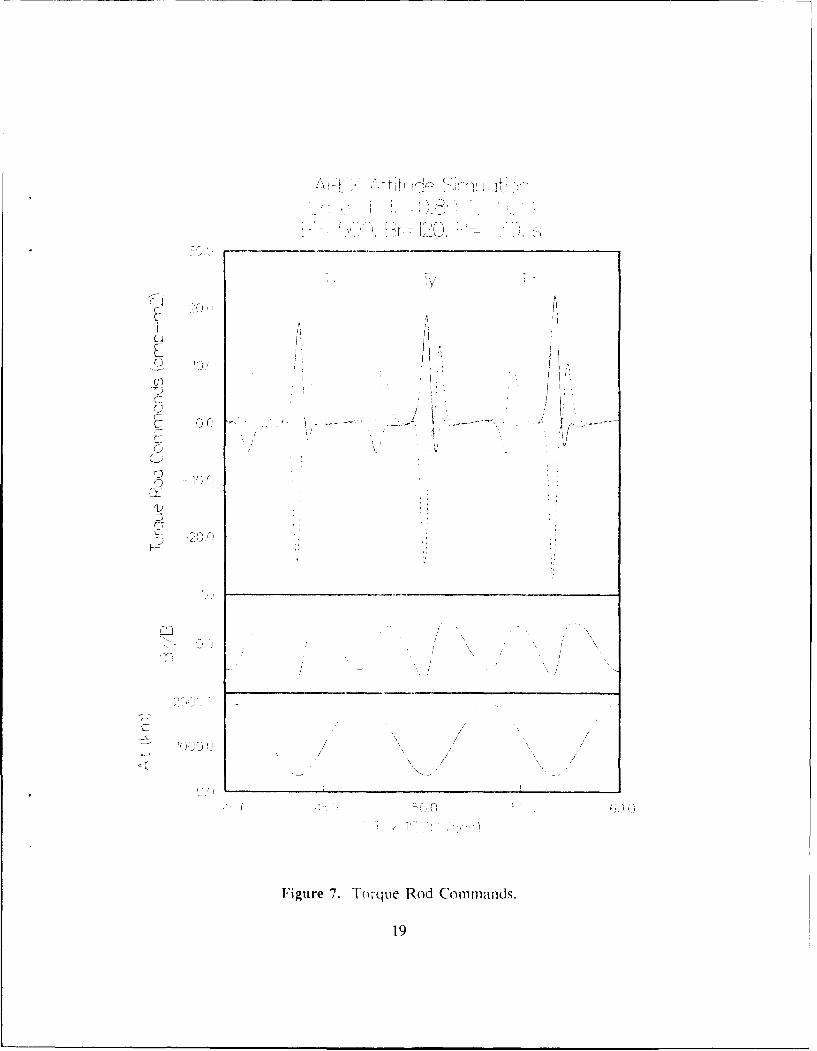
For completeness, we show in Figure 7 the calculated torque rod commands that give rise to theattitude control shown in the previous figures. The torque rods are maximum near apogee andat times when the magnetic field is nearly perpendicular to the spacecraft x-axis, as discussedpreviously. The maximum torques do not exceed the 30 A-mi2 limit imposed by their design.

Finally, in Figure 8 we show the pitch and yaw angles during a series of orbits in which thereis an eclipse. The eclipse period is shown by negative values of the solar depression angle inthe bottom panel. The roll angle in this case is not substantially different from those shownpreviously. This is merely one example of what the attitude behavior might be during eclipse,and substantial variations may be expected due to position of the eclipse within the orbit and themagnitude and time dependance of the induced fields. First, there is a sharp transition fromhigh precision sunlit attitude control to eclipse attitude control. This is reasonable since theattitude is controlled with relatively high precision by the attitude values calculated on-board.These change discontinuously as eclipse is entered due to the errors introduced by induced fields.More importantly perhaps is the realization that the excursions of the attitude from nominalvalues during eclipse is dependent mainly on the induced fields. Since these cannot be wellpredicted at this point, and since attitude determination during eclipse must necessarily involvethe parameterization of the attitude behavior over time, it would seem best to limit a prioriassumptions about the attitude behavior as much as possible. We return to this point when wediscuss the attitude solution in eclipse.

17

APEX Attitude 5"r mulktionr°e 1 TC, -- 0 " 1- -,= " ".:

Variable Static iduced2.5

2.0 Bi=100 Bi=200

1.5 Bi=500

10 -'

0.0

-05

-1.5'

40.0 4, . 440 46.0 4DC 0 ro C ' -_4 . 600Tnrqe 1Qi 00 Wo,-o)"

Figure 6. Roll axis attitude with various static induced fields.

18

_ J A

[ '

c i '

7j

i

I-.

Figure 7. Torque Rod Commands.

19

APEX Attitude SimulatuC,•Case 9 Tc-0.80 Ts-.O29BI= 200. Br•20. P= 3.C S,

A.6

0.2

- 0.0 '/

-0.2(I)

N /,0 -0.4 i -I

c-- I

C-F

Q -0.6

02

-0.8 /K

1.0

2000.0 /,, /

ij /

Figure 8. Pitch and yaw angles for an orbit with eclipses.

20

3.8 SIMULATION OF INSTRUMENTS

The simulation of the data stream from the satellite is quite straightforward, given theassumptions of this model. The times chosen are 60 seconds apart at some arbitrary wholesecond. All measurements are assumed to be coincident in time. The magnetometer values arederived from

Mi = TRUNC([bt,i I bid, i + 60000.0]/g, + 0.5) (38)

where TRUNC reduces the number to the nearest integer of lesser value. gi is the gain factorfor the magnetometer ?ais in nT/count. In this work, we will make the assumption that all gainfactors are equal, but that the gain factor is unknown. As some justification, we cite themagnetometer aboard CRRES. There, gains were matched to approximately .08 nT/count withgains at approximately 22 nT/count. In a field of 30,000 iT, this amounts to approximately onehundred nT maximum, which is near the expected n, ",. level of the system. Should it appearfrom ground test data, however, that the gains of the instrument are substantially mismatched,the calibration algorithms could easily be modified by multiplication of two of the sensors bythe ground measured ratios. The nominal gain of the instrument is 1.831 nT/count.

The sun sensor values are taken directly from the values of pitch and yaw, since these are directmeasurements for APEX. The natural mcasurements of the sun sensors are [Space Sciences,1991] the tangents of the angles

r. -tanO, r, = tanOv (39)

The full scale value of the sun sensor N is 20479 and the digital signal produced is

n = TRUNC( r/ 5 + 10240 + 0.5) (40)

where2 tan~max (1o = - -= 2.002450(-4) (41)

N+l

when 0 max is 640. The sun sensor values are inserted in the simulated telemetry whenever thesolar depression angle is greater than zero. Also produced is a flag which indicates whether thesun sensor can see the sun.

21

4.0 ATTITUDE SOLUTION ALGORITHMS

Having simulated the satellite orbit, attitude and instrument readings, we now turn to algorithmsfor processing these signals. Attitude solutions for APEX come entirely from combinations ofsun sensor and magnetometer readings. In sunlight, the pitch and yaw angles are measureddirectly from the sun sensor data, with roll being calculated from these angles and the magneticfield measurements. In eclipse, all three axes are calculated from magnetometer data alone.Hence, it should be apparent that the calibration of the magnetometer is of critical importancein the enhancement of the accuracy of the attitude calculations. We deal with this issue first.

4.1 MAGNETOMETER CALIBRATION

In our simulation, the magnetometer is assumed to be aligned perfectly with the spacecraft axes,but to have unknown offsets, different for all three axes, and an unknown gain factor, which isequal for all three axes. The measured counts in each axis will be converted to the field in nTalong the axis through the expression

bi = Mi * g - di (42)

We are somewhat limited in the use of on-orbit calibration methods by the fact that the satellitedoes not spin and remains more or less fixed inertially in all three axes. Calibrations can becarried out by comparison of the magnitude of the measured field with a model field. Thismethod involves minimization of the function

F(gd',dydz) = E [b2 - (gMx -dx) 2 - (gMy -dyd)2 - (gM Z -d) 2 ]2 (43)

with respect g and the di's, where bm is the magnitude of a model for the field at the satelliteposition. In principle, a single minimization could be carried out on all four variables, however,the problem is better conditioned if we alternate between minimization of the gain g and theoffsets di. Minimization is carried out by finding the zero of

1dF 2 2 _ (gMy _-d)2)- (gM. -d..) 2d-(44)4 dg f. - (44)

X [ (gMx - dx)M x + (gMy - dy)Ml, + (gMz - dz)M.J

for the gain and

I dF -fx : O --(gM d gM-d) 3

4 ddý, , ) ,(M (45)-E_ (gMý'-d,) (gMy -dy)2-, (gM, -adx)(gM - dz)2

for the offsets. These are quite easily carried out by a Newton-Raphson search technique.

22

In order to test this algorithm, we selected a relatively short portion of data comprising aboutthree orbits. Static induced fields were set at about 200 nT and random high frequency fieldsat 120 nT along each axis. The procedure would most likely be carried out infrequently oversmall portions of a day's data, as was done here. The calculation took initial guesses of g = 1.8nT/count and di=60,000 nT. Figure 9 shows the difference in measured and model field withcalibrated and uncalibrated results. The header shows that the gain is calculated to better than1 part in 2000. The values of di in the header represent 60,000 plus the static induced field (orcalibration error). The twice-per-orbit oscillation in the lower uncalibrated panel is the effecton which the calibration algorithm relies. It is the result of variation in the direction of thebackground field with respect to the induced field, which stays relatively constant in inertialspace.

It is perhaps not too impressive at first glance that calibration has reduced the error from amaximum of 300 nT to 150 nT or so, however, the 150 nT error in the top panel is almostentirely the result of the time varying induced fields, which we were never expecting to remove.Also, it is satisfying to note that the method works when static fields (calibration errors) are notsignificantly larger than the random components. A second example is shown in Figure 10.Here, we have assumed a static component of 500 nT in magnitude. For reference, staticinduced fields on the CRRES satellite were measured at around 200 nT in magnitude. CRRESwas, however, a particularly clean satellite. On the other hand, the magnetometer on APEX issituated 24" from the payload shelf, which reduces magnetic contamination. In practice, thedifferentiation between static and variable fields may not be straightforward. It may well turnout that certain long period events, such as ground transmission, cause large static fields duringthe duration. It is possible that these events could be identified in telemetry, and calibrationcould be carried both with and without, giving an extra set of offsets that could be used duringthe interval to improve the resulting magnetic field and attitude.

We should take note of a couple more things in relation to magnetometer calibration. First,plots like Figure 9 can be very useful in assessing the magnitude and frequency of inducedfields, which we have seen can effect attitude control and which will turn out to be importantin the assessment of the accuracy of the attitude determination. A final point pertains toalignment errors in the instrument. The procedure above does not rely on the alignment of theinstrument with any particular spacecraft axis, but the resulting attitude and measured magneticfield when used to calculate pitch angle certainly do. We do not propose on-orbit calibrationsfor alignments. However, alignment test results should be available with which one can putupper bounds on the errors. Presumably, these will be insignificant. For reference, theengineering magnetometer aboard CRRES was aligned to about one-quarter degree.

4.2 ATTITUDE SOLUTIONS IN SUN LIGHT

When the satellite is in full sun, we have at our disposal two measiired vectors in the spacecraftframe, the sun and the magnetic field. A straightforward and standard technique [Wertz, 19781that can be used for three-axis attitude in this case is as follows:

23

APEX Magnetic Field Calibr-ationG=.830865 Dx=60098 Dy=60038 Dz=59855

400.0

300.0

200.0

o 100.0 A

(9 0.0

-100M0

-200.0

400.0

300.0

200.0 Ao 100.0 A

S0.0 ',

-100.0 "

-200.0

-300.0 I

0.0 2.0 40 6,O 0.0

U I x t )(( (,,

Figure 9. Difference between measured and model field with a 200 nT induced field.

24

APEX Magnetic Field Qalir t or(-010 ' D .f KJ._, Dy 4)111 0 ,

800.0

600.0

400.0

-200.0

-400,0

-6000o

Fie 2 0. Sae

-200.0

-400.0 *jf AJA

-600.0 II

S00. 0 , 10 ./' 1 0

ii 1O) 1•

Figure.0. Sam asFgr u iha 0 Tidcdfed

_,ooo . •25

A triad of vectors is formed from the sun vector s and the magnetic field vector b

a =SS= sxbli x blI (46)

in both the body frame (B) and, using models for sun and magnetic field vectors, in the inertialframe (I). Forming the matrices

Mb = [UB VB WBl M 1 =[U1 VW 1 ] (47)

we can specify the attitude matrix completely by

AM, = MB (48)

and because of orthogonality

TEM (49)A = MBMIt(9

giving a simple and unique solution for the attitude. From there, the results of §2.2 can be usedto obtain pitch, yaw and roll. Since we use the sun vector as a basis vector, the resulting pitchand yaw are identical to the measurements of the sun sensor and the inherent high accuracy ofthese measurements has been preserved by the algorithm.

We should note that the OSC algorithm for calculation of roll angle in sunlight differs slightlyfrom the one presented above [Orbital Sciences, 19921. Their method involves calculating theangle between the magnetic field measured in the yz-plane and the field in a sun and eclipticcoordinate system. The two methods become identical when the satellite x-axis points directlyat the sun and the difference in roll is negligible whenever the values of pitch and yaw are lessthan a few degrees.

To explore the results of this algorithm on the simulated data, we chose a relatively strong staticinduced field of 500 nT and a 120 nT time varying field with frequency high enough so that thefield appears as noise in the magnetometer data. Figure 11 shows the pitch and yaw angles thatresult from the above scheme and the deviations of these results from the actual pitch and yaw.The errors are near the noise level of the sun sensor, since these are direct measurements. Theuncertainty in the values of pitch and yaw during sunlit operation, then, will be limited by theresolution of the sun sensor. In practice, this limitation would also include mounting errors.Judging from measurements of the alignments for the CRRES satellite [Ball Aerospace, 1990]it would appear that typical values for this error are somewhat less than 0.20. Since this is muchgreater than the resolution of the instrument, we will assign a probable uncertainty of pitch andyaw in sunlight to around 0.20.

26

AF0EX Attitude -- Case,-Hr - U /"10. P -

( ) ( )!

,0.005

10

0.8

0.6

0.4

N 0.2

"¢% -0.2 .- ,/ i

-0.4

-0.6

-0.3

10.0-iOii x 1(200 (s-c)

Figure 11. Pitch and yaw angles and errors, computed in sunlit operation.

27

Moving on to the roll axis, we show in Figure 12 the roll angle during the same period.Concentrating first on the actual roll, we sef 'hat the static field of 500 nT has introduced acontrol error of up to four degrees in roll. ., notable aspect, though, is that when roll iscalculated without correction for this static field, the value of roll appears to be substantiallybetter than it actually is. This is because the same erroneous cffsets were used in the controland in the calculation. This result emphasizes the importance of adequate magnetometercalibration for attitude knowledge, and points out the danger inherent in the use of on-boardsolutions without verification. Moving on to the calibrated solution, we see another interestingresult. Although the solution is in agreement with the actual roll on average, it exhibits thesame sort of random jumps as does the uncalibrated solution. This is due to the time varyinginduced field component, which is not removed by calibration. It is interesting that the actualroll does not undergo these oscillations. As discussed before, the control mechanism acts as afilter for high frequency modulations whenever the period is shorter than the time it takes thcsystem to correct for an attitude error. Finally in Figure 13 we show the error in the rollcalculation for this case, using the calibrated magnetic field data. The degree or so error istypical of the maximum effect of a 120 nT field.

It appears, then, that we are able to calculate the roll axis in sunlight to an accuracy limited bythe "unremovable" spacecraft induced fields. It should be kept in mind, though, that themagnitude of these fields are at present unknown. The case presented above is unique to aninduced field of around 100 nT. Repeating the above case with values of Br set at 200 and 500nT leads to maximum errors of 2.50 and 5.0' respectively. The nature of the "unremovable"induced field can be inferred to some degree from compatibility tests as well as on-orbitevaluations by observation of the variation of the measured magnetic field values.

Another issue of importance so far as error analysis is concerned arises from errors in theephemeris and/or timing of the measurements. Whenever a relatively rapidly changing vector,such as the magnetic field, is used for reference, there is an error relating to the difference incalculated position and time and actual position and time. This is quite easy to investigate inthe simulation by substituting the magnetic field calculated for a later time in the attitudedetermination. Figure 14 shows the results of this investigation. Figure 14 was generated withno induced fields at all, so we would expect all the error to be due to timing. This figure alsoserves to demonstrate the integrity of the simulation and calculation, since it shows an extremelysmall deviation due to the 1.8 nT resolution of the magnetometer in the simulation. For I and2 second errors in timing, we see maximum errors of around 0.2 and 0.5 degrees respectively.For reference, the accuracy of the ephemeris will probably exceed 5 km in-track error [McNeil,1992]. This puts the probable error from this source at around 0. 1 degree maximum, since itamounts to about one-half second timing error.

Finally, the issue of the accuracy of the model field is always of importance when dealing withattitude derived from magnetometer measurements. It is our belief that a full IGRF model fieldextrapolated to date yields a field vector that is accurate to about 0. 1 below, say, 4000 km orso. However, there are others who would set this error as high as 1.0'. Attempting to combinethese error sources yields but one unknown, the "unremovable" induced fields. Using CRRES

28

APEX Attitude - Case 2Bi= 500. Br-120. P- 5. s

6.0

Actual Roll Angle5.0

Calbrated Calculated Roll

1t.0

i; 0

S4.60 6.0 &.0 10.0 12.0 14 0 16 0 18.0 20.0

UT Y' 1000 (e'

Figure 12. Roll axis angle, actual and calculated with and without calibration.

29

APEX Attitude - Case 7Bi= 500. Br--120. P=3. s

2.0

1.5 (calibrated Magnetorrieter)

1.0

0.5

0.5

140

-2.00.0 5.0 !.0 Y0

Figure 13. Roll axis error in sunlight with calibrated magnetometer.

30

/-r9L F AttitLde - CB- 0. Br" (. 0. ,

ýj. 4

0. 4

"lcD ,r-r,

-0(.1 I I I I I

, 4.0 6.0 e) 10.0 12, ill IM 1Q) "00

I-f !OOO (e000

Figure 14. Roll axis error arising from errors in timing or ephemeris

31

again as a reference, the fields will be something around 100 nT at the magnetometer. Addingthe ever present mounting error of 0.20 and taking the higher of the estimates for model fielderror, we find that the error in the calculated roll in sunlight may reach as high as 3'.

4.3 ATTITUDE SOLUTIONS IN ECLIPSE

Before describing a solution method for the attitude during eclipse, let us take a closer look atthe attitude behavior. Figure 15 shows pitch, yaw and roll during one typical eclipse andslightly before and after. The eclipse actually begins at around 6200 seconds and ends at about7600 seconds. A rather large static induced field of 500 nT was chosen for this run in order toaccentuate the deviations from nominal operation. As the satellite enters eclipse, we see theeffects of induced field in larger deviations in the pitch and yaw. Of note, however, is the factthat these deviations are relatively smoothly varying in time, depending for the most part on thedirection of the magnetic field relative to the spacecraft. After entering sunlight again, we seethat the control mechanisms require about four minutes to return pitch and yaw to near zero.

One of the most important aspects of the attitude solution during eclipse is that the onlyreference vector available is the measured magnetic field. One reference vector is not enoughto uniquely specify the attitude at any moment. Therefore, a series of measurements must becombined to yield an attitude estimate. There are two popular methods of doing this [Wertz,1986]. These are batch estimators and Kalman filters. In a batch estimator, a model of theobservations, in this case the magnetometer readings taken during a certain period of time, iscreated from a parameterized state vector x(t). These model measurements gi(x(ti)), are thencompared to the actual measurements yi. The loss function

J = Ei [yi - gi(x(ti))]2 (50)

is minimized with respect to the state vector x in its particular parameterization. The model mayvary in complexity from a constant attitude to one which includes derivatives of the state vectorbased on modeled environmental and control torques. The Kalman filter estimates the statevector x(tk) based upon the measurements yi up to and including Yk, and on changes modeledand/or measured in the state vector between measurements.

We have opted for the batch least-squares approach for several reasons, although a Kalman filterwill be used for on-board attitude calculation. First, we have seen that an induced field can leadto a relatively rapid change in attitude at the beginning of eclipses. Since the Kalman filterwould require pre-eclipse data while the least-squares would not, using the later relieves us fromany problems arising from a sudden attitude change. Also, in processing data by APEX periods,which may well begin or end in eclipse, a Kalman filter would require us to save data fromother periods and to process sequentially while a least squares type would not. Finally, sincepost-flight attitude computation is intended mainly for verification of the on-board attitude, itmakes some sense to employ an entirely different method because, as we have seen, attitudecalculation and control are intimately linked.

32

AREX Attitude rc., 9c Tco0.80 . "

9.'5- ,%00. Br- 0. PF 1. s

S1)

(A Ai

' " m'

/

.0 6.0

Li./

7 C

(i-

UT , D!0 O (se,:

Figure 15. Pitch, yaw and roll angles during an eclipse.

33

Another thing to consider is that the complexity of the model g(x) is generally inverselyproportional to the difficulty in obtaining convergence. In the present application, a simplemodel that achieves reasonable accuracy with relative ease is preferable to a more complicatedone of higher accuracy but which is more sensitive to initial guess and requires more carefulconvergence, since the adopted method may have to be run repeatedly in Latch mode. Arecalcitrant model could easily bog down the data processing. The model presented here hasbeen designed with these considerations in mind.

In the simplest possible approach, we can approximate the attitude as a constant over someinterval. The attitude is modeled in ECI coordinates by the right ascension Ot and declination6 of the spacecraft x-axis and by a phase 0 of rotation around this axis. One representation ofthe attitude is [McNeil and Singer, 1986]

cosoecos6 sir "cos6 sin6

A4 = sincosasin+ sinucos,• sin~sincasinc, -coscycosý -cossinoj (51)

_sin~cosoacos - sinusin(ý sin~sincucoso cosusin( - cosbcoso

This parameterization has been chosen so that the nominal vJues of the attitude correspond toU•S= and 6=6., the right ascension and declination of the sun, ,;=0 in configuration 1 and,= 1800 in configuration 2. The function to be minimized is taken to be

I = K (nxi -xbi)2 + Ji (mt, _.-bi)2 + Ei (min 1 - ý'bj)2 (52)

where m, is the i'th component of the measured magnetic field and bi tihe 'th component of thefield in inertial coordinates. The function is minimized by finding the zeros of the threesimultaneous equations, the first of which is

F - T" =E, (m.i - br,,C.C 3 - b, S.iC6 - b-iS3)(bV,1SfC6 - byiCC)

,(, , - ,,C SS - b a.jS ,Co -b aS6S¢, -+ by. C .C O b bz~iC 6S ))x

( .,S 5S) - hXiCCo -h CSS - b S SC)

S- ', SCS, b., h C,,SS h' CSSd C, - +C, j .,CCo)X

Where C stands for cosine and S for sine. The other two equations, F6 and Fo are obtained inthe same way by differentiation of Eq(52) with respect to the appropriate variable. In thealgorithm, the solution is found by a Newton-Raphson search technique, using numericalderivatives of the F,. As a first guess, we assume that the spacecraft x-axis points at the sun andthat the phase angle is zero. This calculation is carried out in a moving window, wth theattitude at the midpoint assigned the v'.lue of the result of the calculation at that window. Inorder to include points at the beginning and end of the eclipse as midpoints of a window, wesimply start a few minutes before Lnd end a feA minutes after the eclipse.

34

In the following paragraphs, we explore the behavior of this solution in the various situationsof the test cases. In the first example, we assume, a 'random' field of 120 nT to test theresponse of the solution to noise. After that, we set the 'random' field to zero to better assessth,." characteristics of the solution without this complication. The static field is taken to be 500nT and results of calibration of the magnetometer, discussed earlier, are used in all calculations.As we recall, 500 nT is probably somewhat excessive and constitutes therefore a 'worst case'insofar as the deviations of satellite operation from nominal.

In Figure 16 we show the solution for the eclipse presented in the previous figure. In one sense,at first glance, it is somewhat disappointing that we see errors of a degree or so in quantities,pitch, yaw, and roll, that are themselves only a few degrees in magnitude. However, we shouldconsider these results in light of the inherent difficulty of specifying a changing attitude throughthe use of a set of single vector measurements. This is never a very happy situation. When theattitude changes, the best solution may not be the average attitude throughout the window. Wehave selected a seven minute window for Figure 16. Reduciig the window would allow for asomewhat better result, but would also increase the noise level due to the random fields. Witha three parameter model, we can use as few as three points. The actual choice in practice willdepend to some extent on the noise level of the instrument. In any case, we can certainlyconclude from Figure 16 that the ,-ellite is operating normally, which is the main issue.

The solution is in error in proportion to the rapidity with which the attitude changes within awindow. If the satellite remains within specified operating range, these changes will be smallas in Figure 16 and the solution obtained will reflect proper operation, with errors of a degreeor two. It is also approximately the same as that expected from the 100 nT or so 'random'induced fields. Improvements to the results of Figure 16 do not come easily. Addingparameters for time varying attitude requires increase in the window size for convergence anduniqueness. This in turn simply means that the attitude changes more within the window, givingresults that are not substantially better. We have opted to stick with a constant parameterizationand a relatively short window. In the following, we investigate the associated errors in severalsituations.

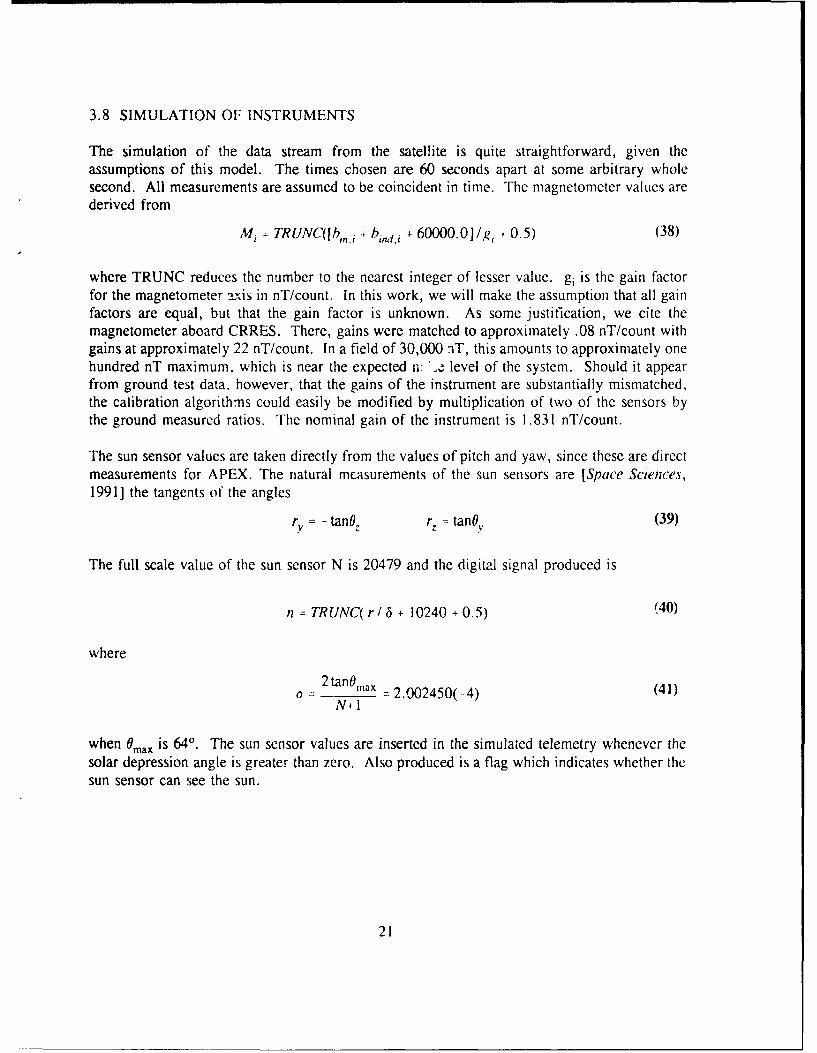
An interesting situation that is in some ways 'worst case' occurs in the second eclipse of Case10. The attitude and the solution provided by the above algorithm are shown in Figure 17. Wehave chosen a three minute window for this calculation, which would be desirable wheneverchanges in attitude are greater than the instrument noise level. The effect is concentrated in theroll axis (0,) which can be seen to change rapidly at around 10,300 seconds UT. The reasonis as follows. At that time, the magnetic field vector becomes nearly parallel to the spacecraftx-axis. This means that the spacecraft induced fields create a disproportionate angular error inthe calculated roll. Even thot gh the inclusion of induced fields in this simulation is somewhatartificial, there seems to be no reason why this effect should not be observed in practice to someextent. As the error increases, first in a positive sense then inflecting to the negative side, thesatellite compensates for the erroneous calculated roll. Compensation and hcnce attitude changein the roll is rapid since the momentum wheel can act somewhat more efficiently than can thetorque rods. Thus this effect would not be observed to so great an extent when the magnetic

35

APEX FEcipse, consstant w/ :;S.Case 9 Eclipse #

1.0

.7

0.5 /

o• 0.0 v //""

0.0

-0.5 ,

"0 •"-- --"I

6.0

4.0

x, 2.0

0.0

-2.0 I

6.0 6.5 7.0 7± S 0

Time x 1000 (sec)

Figure 16. Best fit constant attitude solution with 7 points/fit.

36

APEX Eclipse, constant w/' -ý ps.,se Ec lpse /#

2.0

1.0 / /

Jo./.l /

0' V

V

0.0

» -2.0 //0

-4.0

15.0

10.0

5C~ A

/ ^/

-01.0 I I . C" 1I

Timrn x 100e (sec),

Figure 17. Attitude and solution (dots) for Eclipse 2 of Case 10.

37

field is perpendicular to the spacecraft x-axis instead. Although the solution has pretty muchmissed the rapid roll change, it at least reflects some aberrant behavior in roll.

Although this case gives rise to a rather large angular error in the calculated attitude, it too mustbe considered in light of the possibilities at hand. We believe that there is virtually no way todo substantially better when the attitude changes by 100 or so in the course of a few minutes.At least the solution has produced an attitude that is within a couple of degrees of correct forthe x-axis (0y and O0) and has given us something near the average for the roll. This brings upanother feature of the parameterization worth mentioning. The values of a and 3 are determinedprimarily from the measurement of the spacecraft x-axis magnetic field. Had we solved usingonly these two parameters, that is,

J - (m,,i - (x. bi)) 2 (54)

we would have obtained almost identical results to those in Figure 17. This is nice in that theremay well be motion in roll that is not echoed in pitch and yaw, and vice versa.

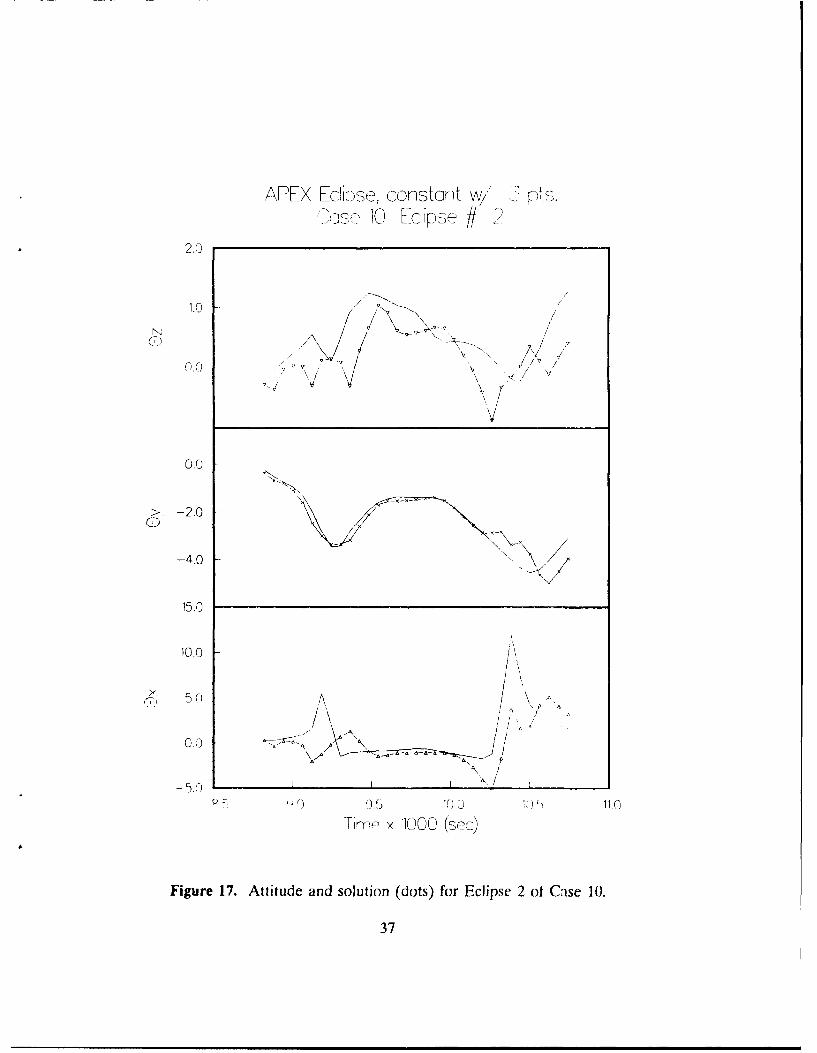
We should also test the solution algorithm on some very anomalous cases, since one of the majorobjectives of post-flight attitude determination is to verify nominal operation. One way tosimulate non-nominal behavior is to increase the value of the static induced field B1 . In Figure18, we show an eclipse for which Bi=2000 nT. Again, since changes in .:ttitude are large, wehave used a short window. In this case, the roll and 0y both exceed the 50 nominal limit.Although the rapid changes in roll cause the roll axis to be calculated with errors of up to about50, we see again that the error does not propagate strongly into the pitch and yaw calculations,where errors are nearer 20. More importantly, the fact that the attitude exceeds the nominallimits in this case is evident from the calculated results. The last four points are, as usual, insubstantially larger error due to the fact that they require post-eclipse points for their calculation.The pitch and yaw change rapidly after eclipse, recovering the sun within about four minutes.

As another test of the method in extremes, we look at the attitude that results from abandoningall attempts at control during eclipse. One such eclipse and the resulting solution is shown inFigure 19. We see that the pitch and yaw are relatively constant throughout and the roll errorincreases about linearly as the momentum wheel transfers the spin of the pitch and yaw axes tothe roll axis. Although this is probably not an actual operational possibility, it is similar to theso called 'safe-hold' mode that will go into operation as a result of numerous anomalousconditions. In this mode, the roll axis is not controlled at all and will drift as in Figure 19.Pitch and yaw are controlled through torque rod operation and should remain small. We see inFigure 19 that the rapid change in roll (or 4) leads to errors of about 20 in the pitch and yawdeterminations.

When in safe-hold mode, or at any other time when variation in roll greatly exceeds variationin pitch and yaw, there is a simple way to increase the accuracy of these solutions. If we letthe variable 4(t) be parameterized by a constant and a linear term,

38

APEX Eclipse, constant w/ 3 pts.Case 10 Eclipse # 3 BI=2000y

6.0

4.0

N 2.0 /,- \N

0.0 /

-2.0 ,

2.0

0.0

-2.0 -

o -4.0-

-6.0 -x

-8.0

20.0

15.0

10.0

xo 5.0 -

0.0 \

-5.0

-10.0 I I

15.0 15.5 16.0 16.5 17.0 17.5Time x 1000 (sec)

Figure 18. Attitude and solution (symbols) for a non-nominal case.

39

APEX Eclipse, constant w/ 7 pts.Case 8 Eclipse # 8

1.0

0.0

N ,.///

oD -1.0

1.0

0.0

o -10

-2.0

5.0

0.0

-10.04/0 47.5 -48.0 48 .

Time x U000 (sec)

Figure 19. Attitude and constant solution for no control during eclipse.

40

0b(t) = •0 + Olt (55)

and minimize with respect to the four variable parameterization, we obtain the results in Figure20. Due to the clean separation of .0 from a and 6 in the problem, this set is also quite easy tominimize without convergence problems. As can be seen, the solution is quite good, until thefinal few points which suffer from the rapid reacquisition of nominal attitude immediately aftereclipse. We will include this option in the solution package for use in safe-hold mode. Sincechanges in roll under normal operating conditions are often no more than those in pitch and yaw,use of this method there would probably not result in substantial improvement.

In summary, it appears that this method is capable of producing results accurate to around 2-3'when the attitude stays within nominal operational constraints. The method will thus be adequatefor verification of nominal operation. Should the attitude stray greatly from nominal duringeclipse, the error inherent in the calculation also will increase, at least with larger rates ofchange of the attitude parameters. However, the resulting attitude appears to be of adequatequality to judge the approximate degree of deviation from nominal. Errors are approximatelythe magnitude of the change in any attitude parameters within the window. In safe-hold mode,the addition of a linear term in roll removes the error due to rapidly changing roll. Thesealgorithms appear as the methods of choice, since they are adequate for control assessment, donot require initial values and are rapidly convergent.

5.0 EVALUATION OF ON-BOARD ATTITUDE

In addition to the verification of nominal operations, we must decide in the course of attitudeprocessing whether the post-flight or the on-board attitude best represents the actual attitude.Discretionally, either one or the other will be included on Agency Tapes for the perusal ofexperimenters. During sunlight operations, this decision presents no great problem since,barring magnetometer calibration problems, the two solutions should be identical. The decisionthen shifts to one of which set of calibration factors are the best. This can be evaluatedindependently by comparison with model fields.

In eclipse, we are faced with a more difficult problem. What, for example, if we plotted theon-board and post-flight solutions and came up with something like Figure 16, with agreementto about 2-3"? There is a way by which we can at least verify the self-consistency of the on-board solution. Accompanying the on-board pitch, yaw and roll data will be rates of change ofpitch, yaw and roll. We can use these to approximate the rates of change in a, 5 and 4) andthereby greatly increase the level of accuracy of our parameterization. These rates of changeare given by

41

APEX Eclipse, w/ dq /dt & 7 pts.Case 8 Eclipse # 8

1.0

0.5

-0.5

1.0

0.5

o 0.0

-0.5

5.0

>< 0.0

-5.0

-10.047.n 47.5 48.0 48.5

Time x 1000 (sec)

Figure 20. Same as Figure 19 but with a linear term in 4

42

dot dt dt dt dt

In the eclipse algorithm, we minimize a0 + act, etc. where a1 remains fixed at the reported rateof change given in telemetry. Should this give rise to a solution more like the on-board solution,assuming that both solutions are comparable, we would be inclined to elect the on-board solutionfor Agency Tape generation. Figure 21 repeats the eclipse of Figure 16 but with fixedderivatives obtained from the attitude simulation. Should the on-board and post-flight attitudecome out markedly different, however, the self-consistency of the on-board attitude and ratesis not a sufficient indication of the better quality of the on-board solution.

6.0 CONCLUSION

We have modeled the APEX ephemeris and attitude over the course of several days,encompassing a variety of situations and have observed the response of the satellite usingrealistic environmental and control torques. Using these results, algorithms have been developedand tested for magnetometer calibration and for attitude solution. Although the results of thismodel may well be substantially different from the actual attitude behavior, we believe that therelative success of the computations on simulated data will be reflected in the experience withreal data. The verification of the sun to solar panel angle during sunlit operations isstraightforward and should be accurate to a few tenths of a degree. It appears to be possible tocalculate the roll angle in sunlight and the three attitude angles during eclipse to a precision ofperhaps a factor of two higher than the nominal allowed deviations of 50 in the attitude.Although, for verification purposes, a larger margin would be preferable, the present situationallows for the determination of attitude control with reasonable confidence.

In closing, we should reiterate the importance of this type of simulation in the development ofattitude determination software. Although it may appear somewhat overly complicated and evenrepetitive, since OSC has also performed these types of simulations, it is altogether necessary.Without simulation of the environmental torques along with the restoring torques commandedby the actual control laws, we would be left with considerable uncertainty in the definition ofthe attitude itself. Without simulation, too, we would have no indication of the degree or rateof attitude change during eclipse, and thus would not be able to evaluate the effectiveness of thechosen solution algorithm. Assuming a constant attitude, for example, would have led to aresult in precise agreement with the attitude. We have seen, however, that errors in practicemay be substantially larger, but still tolerable. The fact that we have tested the proposedalgorithms, along with the general familiarity with the expected attitude and sensor dataconferred by simulation, gives us considerably more confidence of successful and expedientevaluation of the actual attitude data, once it is in hand.

43

APEX Eclipse, w/ deravitives 7 pts.Case 9 Eclipse # 2

1.0

N 0.50

0.0

0.0

-0.5

0 1.

-1.5

6.0

4.0

X(3 2.0

0.0

-2.0 i I

6.0 6.5 7.0 7.5Time x 1000 (sec)

Figure 21. Case 9 Eclipse 2 solution, calculated with 'known' rates of change.

44

REFERENCES

Ball Aerospace, "Verification Test Report for Alignment Measurements of CRRES", CRRES-915, Ball Space Systems Division, Boulder, Co., 9 March 1990.

Barnison, R., private communication, 1992.

Kwok, J. H., "The Artificial Satellite Analysis Program (ASAP)", Jet Propulsion Laboratory,Pasadena, Calif., April 1987.

McNeil, W. and H. J. Singer, "Fluxgate Magnetometer Analysis and Simulation Software forCRRES", AFGL-TR-86-0222, 1 October 1986, ADA176353.

McNeil, W., "Software Detailed Design Document for the APEX Orbit~i Dati PioccssingSystem Ephemeris Computation Function", Radex, Inc., Bedford, Mass. (APEX-EPH-02) 20 April 1992.

Orbital Sciences Corp., "APEX ACS Code Walkthrough", Fairfax, Va., 30 April 1992.

Space Sciences Corp., private communication, 1991.

Stoltz, P., "APEX Critical Design Review: Attitude Determination and Control Subsystem",Fairfax, Va., 5-8 November 1991.

Wertz, J. R., ed., "Spacecraft Attitude Determination and Control", D. Reidel PublishingCompany, Boston, 1986.

45

Appendix - State Vectors

The following state vectors were used to generate the ephemeris for this study. Thecoordinate system is true-of-date Earth Centered Inertial.

Year Day Second Rev IX(km) Y(km) Z(km) Vx(km/s) Vy(km/s) Vz(km/s)

91 0 0.000 1 0.00005922.681152 -2312.936035 2227.808838 3.38994217 1.82176983 -7.11462641

91 1 0.000 14 0.0000333.102753 2673.440674 -7309.891602 -6.71503830 2.03565097 -0.30837882

91 2 n.000 27 0.0000-7843.144043 2569.690186 -104.129593 -0.50028402 -2.21145177 6.20766211

91 3 0.000 41 0.0000-34.582718 -2538.974121 6590.689941 7.30961275 -2.06632018 -1.46704304

91 4 0.000 54 0.00005658.311035 -571.851929 -4303.395020 -3.25924301 3.62198353 -5.92411470

91 5 0.000 67 0.0000-4664.481445 4196.505859 -5401.880859 -4.96536970 0.47305381 4.29641962

91 6 0.000 81 0.0000-5845.307617 798.506714 4966.917480 4.15876436 -3.75541592 4.36136055

91 7 0.000 94 0.00005229.038086 -3639.860840 2209.513184 3.78598666 0.92756629 -7.07966566

91 8 0.000 107 0.00001119.718994 2464.516357 -7403.245117 -5.94886065 3.54509449 -0.41860914

91 9 0.000 120 0.0000-6939.483398 4365.214844 -279.218292 -1.07204473 -2.01031303 6.25145912

91 10 0.000 134 0.0000-394.175568 -2558.539063 6460.285645 6.71218014 -3.69477177 -1.67764628

91 11 0.000 147 0.00005339.558594 -1731.985596 -4604.779297 -2.48622346 4.29536104 -5.67568588

47