Embed Size (px)
Citation preview

Auburn University
Department of Economics
Working Paper Series
Forecasting Net Charge‐Off Rates of
Banks: A PLS Approach
James Barth†, Sunghoon Joo†, Hyeongwoo Kim†,
Kang Bok Lee†, Stevan Maglic, and Xuan Shen
†Auburn University; Regions Bank
AUWP 2018‐03
This paper can be downloaded without charge from:
http://cla.auburn.edu/econwp/
http://econpapers.repec.org/paper/abnwpaper/

1
Forecasting Net Charge-Off Rates of Banks: A PLS Approach *
April 2018
* The authors are grateful to the editors for helpful comments that substantially improved the chapter.
James R. Barth Lowder Eminent Scholar in Finance
Raymond J. Harbert College of Business 316 Lowder Hall
Auburn University Auburn, AL 36849
Phone: (334) 844-2469 E-mail: [email protected]
Sunghoon Joo
Ph.D. Student in Finance Raymond J. Harbert College of Business
306 Lowder Hall Auburn University Auburn, AL 36849
Phone: (334) 524-8011 E-mail: [email protected]
Hyeongwoo Kim
Professor in Economics 217 Miller Hall
Auburn University Auburn, AL 36849
Phone: (334) 844-2928 E-mail: [email protected]
Kang Bok Lee
Assistant Professor in Business Analytics Raymond J. Harbert College of Business
424 Lowder Hall Auburn University Auburn, AL 36849
Phone: (334) 844-6512 E-mail: [email protected]
Stevan Maglic
Senior Vice President and Head of Quantitative Risk Analytics Regions Bank
1900 5th Avenue North Birmingham, AL 35203 Phone: (205) 264-7547
E-mail: [email protected]
Xuan Shen Vice President and Risk Quantitative Analyst
Regions Bank 1900 5th Avenue North Birmingham, AL 35203 Phone: (205) 264-7750
E-mail: [email protected]

2
Abstract
This chapter relies on a factor-based forecasting model for net charge-off rates of banks in a data-
rich environment. More specifically, we employ a partial least squares (PLS) method to extract
target-specific factors and find that it outperforms the principal component approach in-sample by
construction. Further, we apply PLS to out-of-sample forecasting exercises for aggregate bank net
charge-off rates on various loans as well as for similar individual bank rates using over 250
quarterly macroeconomic data from 1987Q1 to 2016Q4. Our empirical results demonstrate
superior performance of PLS over benchmark models, including both a stationary autoregressive
type model and a nonstationary random walk model. Our approach can help banks identify
important variables that contribute to bank losses so that they are better able to contain losses to
manageable levels.
Keywords: Net Charge-Off Rates; Partial Least Squares; Principal Component Analysis; Dynamic
Factors; Out-of-Sample Forecasts
JEL Classification: C38; C53; G17; G32

3
1. Introduction
Banks provide important products and services to individuals and firms in countries
throughout the world. Their goal is to serve their customers while at the same time earn profits that
are acceptable to the shareholders. As banks attempt to accomplish these tasks on an ongoing basis,
they must necessarily balance risk and return. Too much risk can lead to failure, while too little
return can disappoint shareholders. This means that banks are constantly engaging in a balancing
act as they try to achieve an acceptable tradeoff.
Banks, however, do not choose the tradeoff between risk and return by themselves. Instead,
various bank regulatory and supervisory authorities assist, and sometimes quite forcibly, in this
effort. More to the point, banks in countries everywhere are highly regulated with respect to many
of their business practices to promote safer and sounder banking systems. Serious trouble arises
when a bank incurs losses that deplete its capital. When such a situation is widespread throughout
the banking sector, as occurred in the U.S. in 2007-2008, the result is a banking crisis, which can
lead to bank bailouts, which actually happened in the U.S. in the Fall of 2008. Worse yet, this can
lead to a severe recession, as also occurred in the U.S. from late 2009 to the summer of 2009.
To avoid individual and widespread bank losses, and associated failures, banks try to
identify those variables that are most likely to contribute to the most losses, which better enables
them to contain the losses to manageable levels. They have every incentive to do so otherwise the
outcome may be their eventual closure, or even seizure by the regulatory authorities, with adverse
outcomes to shareholders. In addition, the authorities and accounting guidelines require that a
procedure be in place for forecasting losses. In particular, banks will provision for anticipated
losses on loans and thereby build up a reserve for loan losses. Regulators and auditing firms can

4
then evaluate whether the allowances made for such losses are adequate for likely future financial
and economic developments.
The purpose of our paper is to evaluate the forecasting accuracy with respect to bank losses
of a partial least squares (PLS) model as compared to two simpler benchmark models. Although
there may be other approaches, the advantage of the PLS model is that it allows one to include
more predictor variables than observations in forecasting a target variable. This is clearly likely to
be the case in the banking industry, with local, national, and in some cases international, factors
affecting the performance of individual banks as well as the entire banking system. Our specific
focus is on forecasting bank losses, or net charge-offs, using a PLS model and comparing its
performance to the benchmark models. Typically, when one tries to identify predictor variables,
the number is restricted to be less than the number of observations. However, in reality, as already
noted, there are generally far more variables that can affect the net charge-off rates of banks than
the number of available observations in any forecasting exercise. We therefore use a PLS model
to obtain forecasts for net charge-off rates for all banks and two very big banks based on more than
two hundred predictor variables, as discussed in more detail below.
The remainder of the paper proceeds as follows. In the next section, we review thirteen
articles in several business disciplines that use partial least squares in an empirical analysis. As
will be seen, there is a relative paucity of studies using this technique in the banking literature. The
third section describes and explains factor-based forecasting models with partial least squares,
including those used in this article. It also contains our basis for choosing the best forecasting
model for net charge-offs of banks. The fourth section contains our empirical findings regarding
forecasts over various horizons and an evaluation of forecast accuracy based on a comparison of
the PLS model to the benchmark models. The last section contains a summary and conclusions.

5
2. Literature Review
Based upon a check of relatively recent articles, we were able to identify thirteen papers that use
PLS in an empirical examination involving several business disciplines. In particular, we found
three articles focusing on accounting issues, one article addressing retailing branding, four articles
that deal with more general finance topics, and five articles that are in the banking industry and
therefore more closely related to our paper. Admittedly, there no doubt are other papers in various
business disciplines that also use PLS, especially in the accounting field, as noted in a few of the
papers we review.
Of the three accounting articles, Lee et al. (2011) explains the benefits of using PLS as well
as compares and contrasts it with both ordinary least squares and covariance-based structural
equation modeling. Moreover, general guidelines are provided for the usage of PLS and its use in
the accounting literature is discussed. The authors point out that the usage in accounting has been
limited, though much of the usage has conformed to best practice guidelines. In a related vein, Goh
et al. (2014) discuss how partial least squares-structural equation modelling can be used in archival
financial accounting research. They also point out that PLS is a non-parametric method that is
suitable for non-normally distributed data in an analysis, which prior empirical studies find is often
the case. The third accounting article by Larson and Kenny (1995) was published nearly thirty
years ago and empirically examines the relationship between developing countries’ equity market
development and economic growth due to the adoption of International Accounting Standards.
Based on PLS, they find that the mere adoption of such standards does not guarantee greater equity
market development or economic growth. In the fourth accounting article, Nitzl (2016) emphasizes
the importance of PLS in situations in which only a weak theory exists and therefore a set of
different possible influences have to be tested. In this respect, it is noted that management

6
accounting research frequently has exploratory elements because the theoretical basis is often
weak. The author concludes that PLS should not be neglected by management accounting
researchers in the future.
Turning to the article on retail branding, or “retail equity”, Arnett et al. (2003) use PLS to
develop parsimonious measures for retail equity. More specifically, they find it to be a useful tool
that can be used to construct an index for assessing the success (failure) of marketing strategies
and tactics, among other uses. The conclusion is that PLS provides a method that yields an easy to
use index that can be employed by both marketing managers and researchers.
The four papers that focus on more mainstream financial issues are relatively recent, all
released or published in 2013 or later, with the exception of one paper published in 2006. The
article by Kelly and Pruitt (2013) is quite important because it tackles a challenging problem in
empirical asset pricing, which is to exploit the information contained in a large number of predictor
variables but limited by a relatively short time series. As they explain, a solution is provided by
PLS, which has the properties in a factor model setting that apply to the asset pricing model
considered by them. The authors note that principal components (PCs) can also be used to
condense information from a large number of predictor variables into a small number of predictive
factors. However, PLS condenses the predictors according to covariance with the forecast target
and chooses a liner combination of predictors that is optimal for forecasting. In contrast, the PC
approach condenses the predictors according to covariance within the predictors. Based on this
difference in approaches, Kelly and Pruitt (2013) point out that the components that best describe
predictor variation are not necessarily the factors most useful for forecasting, and therefore PCs
can produce suboptimal forecasts. They conclude that their empirical results obtained from PLS
“stand in contrast” to those implied by standard models of asset prices.

7
The paper by Huang et al. (2015) develops a new investor sentiment index aligned for
predicting the aggregate stock market return. They use PLs in their empirical work, noting that the
method was recently introduced to the finance literature by Kelly and Pruett (2013), which is the
paper just discussed. Huang and coauthors find that their new index performs much better than
most of the commonly used macroeconomic variables do and improves substantially the
forecasting power for a cross-section of stock returns formed on industry, size, value, and
momentum. Moreover, they attribute the success of the investor sentiment index to the use of the
PLS approach that exploits more efficiently the information in proxies than existing procedures
do. This provides further motivation for the use of PLS in our empirical work.
The paper by Lie et al. (2017) also focuses on stock returns, but more specifically on
predicting the stock market risk premium. They point out that Cochrane (2008) emphasized that
understanding the variation in the market risk-premium has important implications in all areas of
finance. The authors new approach is to construct a comprehensive index of corporate activities
that is used to predict the stock market return, but one that is constructed using the PLS approach.
They find that ignoring the information in corporate activities when using PLS clearly impedes the
ability of the asset pricing models in explaining asset returns.
In a more narrowly focused finance paper, Laitinen (2006) demonstrates the use of PLS in
predicting payment default based upon data for Finland. The results indicate that when using only
two PLS-factors as predictors one obtains an equal classification accuracy nearly the same as when
an original eight variables are used. The conclusion is that PLS provides a powerful method to
reduce dimensions in default prediction, particularly when there are many predictors and they are
highly collinear.

8
Given that our paper relies on PLS as the method chosen to forecast net charge-off rates in
the banking sector, we now discuss the use of this technique in the banking literature. In this regard,
five papers have been identified that use PLS. Perhaps the limited number of papers is not
surprising insofar as one of the papers points out that the advantages of this technique have hardly
been exploited in the banking discipline. The author of the paper that makes this point, Avkiran
(2018), provides a discussion of the use of PLS in structural equation modelling as an introduction
to a book entitled “Rise of the Partial Least Squares Structural Equation Modelling: an Application
in Banking”. In contrast, Ayadurai and Eskadurai (2018) actually apply PLS to examine the drivers
of bank soundness in the G7 countries during the period 2003-2013. The empirical results indicate
that based on 17 manifest variables there are six constructs that are a direct cause and eight
constructs that are an indirect cause of bank soundness. In particular, it is found that banks placed
high importance on off-balance sheet and capital activities, and thereby taking on more risk.
An interesting and timely article is by Avkiran et al. (forthcoming). They provide the first
application of PLS in financial stress testing, as far as we know. The specific focus is on the
transmission of systemic risk from the shadow-banking sector to the regulated banking sector. The
empirical results indicate that a substantial degree of the variation in systemic risk in the regulated
banking sector is explained by micro-level and macro-level linkages that can be traced to shadow
banking. They conclude that this is an insight due to the use of PLS.
The last two banking papers addresses issues mainly related to customers. The paper by
Poolthong and Mandhachitara (2009) examine the way in which social responsibility initiatives
can influence perceived service quality and brand effect from the perspective of retail banking
customers. Based on an analysis of the responses of 275 bank customers to a questionnaire using
PLS, the results indicate that perceived service quality is positively associated with brand effect

9
mediated by trust. In the other paper, Bontis et al. (2007) also use survey data based on 8,098
respondents to study the mediating effect of organizational reputation on service recommendation
and customer loyalty. The results obtained using PLS indicate that the relationship between
corporate reputation and profitability may reside in reputation’s influence on customer loyalty, and
that reputation plays an important role as regards customer satisfaction.
In summary, it is clear form these thirteen papers that PLS was the method used to obtain
new and interesting results. The different papers, moreover, identified the advantages gained by
using PLS as compared to the more traditional procedures used in the respective business
disciplines. It was also clear that even though PLS might have considerable advantages it is still a
relatively under-employed method in most of these disciplines, especially banking.
We now turn to an application of PLS in an important issue in banking, namely, forecasting
losses incurred by banks in their normal course of operation accurately to avoid losses sizeable
enough to jeopardize their very ongoing existence.
3. Factor-Based Forecasting Models with Partial Least Squares
3.1. Partial Least Squares Factors
We employ the Partial Least Squares (PLS) approach in an analysis of the net charge-off rates for
banks to extract the target-specific factors from a wide range of variables that influence the
performance of banks for our out-of-sample forecasting exercises. For PLS, consider the following
linear regression model. Abstracting from deterministic terms,
, 1, 2, … , , (1)
where is the target variable, net charge-off rate, , , , , … , , ′ is an 1 vector of
predictor variables, bank-specific and macroeconomic variables, is an 1 vector of
coefficients, and is the random error term.

10
The PLS method is a useful tool, especially when . The reason is when the number
of observations ( ) is less than the number of predictors ( ), the ordinary least squares estimator
is not well-defined. Instead of estimating a full regression with all the predictors given by equation
(1), PLS employs a data dimensionality reduction method via the following regression model.
, (2)
where , , , , … , , ′ is an 1 , vector of PLS components or factors and
is an 1 vector of coefficients. PLS factors are linear combinations of predictors. That is,
′ , (3)
where , , … , ′ is an weighting matrix and its column vector
, , , , … , , ′ is an 1 vector of weights on predictor variables for the factor (
1,… , ).
The PLS estimator chooses that minimizes the sum of squared residuals from equation
(2) instead of choosing to do the same in equation (1). As Andersson (2009) shows, there are
many available PLS algorithms that work well. We use Helland’s (1990) algorithm that is
intuitively appealing to obtain PLS factors for the -period ahead target variable, ,
1,2, . . . , , as described in the following steps.
First, the first PLS factor , is determined by the following linear combinations of the
predictor variables .
, ∑ , , , (4)
where , , , is the loading parameter that is the covariance between the target and
each predictor.
Second, we regress and , on , then obtain the residuals, and ,
, , then repeat the process described by equation (4) to obtain the second PLS factor , . Note

11
that , is orthogonal to , , that is, , contains new predictive content that is not contained in
, .
Repeat the steps described until one obtains all factors, , , , , … , , that are
orthogonal to one another.
3.2. PLS Factor Forecasting Models
We employ two PLS factor-based forecasting models (Kim and Ko, 2017) based on two
benchmark models, the nonstationary random walk model and a stationary autoregressive model.
For notational simplicity, we abstract from all deterministic terms, although all estimations are
implemented with an intercept.
The first model augments the following random walk (RW) model,
, 1, 2, … , , (5)
where ∑ and is a white noise process. The PLSRW model extends the RW
model given by equation (5) by adding the PLS factors as follows.
, (6)
Note that the ordinary least squares (OLS) estimation for equation (6) is not feasible
because the coefficient on is predetermined. To deal with this problem, we regress
on to get the OLS estimate for , . Adding back to both sides, we obtain the -period
ahead forecast from the PLSRW model as follows.
, (7)
while the forecast from the benchmark RW model is,
, (8)
which is nested by equation (7) when 0.

12
The second model uses the following autoregressive (AR) model,
, (9)
where is less than one in absolute value. Note that equation (9) coincides with an AR (1) model
with the persistence parameter when and ∑ and is a white noise
process. The PLSAR model extends the AR model given by equation (9) by adding the PLS factors
as follows.
, (10)
Using the OLS estimates of the coefficients for equation (10), we obtain the -period ahead
forecast from the PLSAR model as follows.
, (11)
while the forecast from the benchmark AR model is,
, (12)
which is again nested by equation (11) when 0.
3.3. Out-of-Sample Forecasting Evaluations
We evaluate the out-of-sample predictability of the target variable using the following two forecast
exercise schemes:
1. We first employ an expanding window (recursive) scheme. Using the initial
observations, we estimate the PLS factors from , . Using the factor estimates, we
obtain the -period ahead out-of-sample forecast for the target variable by equations (7), (8),
(11), and (12). Then, we obtain the prediction errors for each model.
2. Then, we expand the data by adding one more observation and re-estimate the factors
from , , which are used to formulate the next forecast, , which gives another set

13
of prediction errors. We repeat the process until we obtain the last forecast using the last set of
factor estimates obtained from , .
We also employ a fixed-size rolling window method, which may perform better than the
recursive method when structural breaks are present. After the first step in obtaining , we add
one observation but remove the earliest observation in the next step in obtaining , which
maintains the same number of observations (fixed-size window). That is, we re-estimate the PLS
factors utilizing the data , instead of , as in the recursive scheme. Again, we
repeat until we forecast the last observation using the last set of factor estimates obtained from
, .
We employ the ratio of the root mean square prediction error (RRMSPE) to evaluate the
out-of-sample prediction accuracy of our PLS factor forecasting models. RRMSPE is calculated
as follows.
∑ |
∑ |
, (13)
where | denotes the forecasting error from the model which refers to either of the two
benchmark (BM) models (RW or AR) or one of the three competing models (PLS, PLSRW, or
PLSAR). We employ the squared error loss function in equation (13), although the absolute error
loss function could be used. Our PLS models outperform the benchmark models when RRMSPE
is greater than 1.
4. Applications
4.1. Data Description and In-Sample Analysis
4.1.1. Data Description

14
We obtained quarterly data on the net charge-off rates for all banks from FRED Economic Data at
the Federal Reserve Bank of St. Louis website for 1987 Q1 to 2016 Q4. Figure 1 shows the net
charge-off rates on seven different types of loans as well as all loans. Note that there is a substantial
heterogeneity in the rates for the different types of loans over the nearly 30-year period. All charge-
off rates except for loans to finance agricultural production tend to experience relatively high
charge-off rates for several quarters following the banking crisis of 2007-2008 and the severe
recession from late 2007 to the summer of 2009. Note also that commercial and industrial loans
tend to have three relatively high peaks as compared to the other types of loans, which indicates
that such loans are among the riskiest loans.
Figure 1 around here
We also obtained data on 249 macroeconomic variables for the same sample period noted
above from a beta version Fred-QD (https://research.stlouisfed.org/econ/mccracken/fred-
databases/). As Table 1 shows, the macroeconomic variables are grouped into 14 categories. More
specifically, Group 1 includes 23 national income and product account variables, Group 2 includes
18 industrial production variables, Group 3 includes 49 employment and unemployment variables,
Group 4 includes 13 housing variables, Group 5 includes 11 inventories, orders, and sales variables,
Group 6 includes 47 prices variables, Group 7 includes 14 earnings and productivity variables,
Group 8 includes 22 interest rates variables, Group 9 includes 17 money and credit variables,
Group 10 includes 9 household balance sheets variables, Group 11 includes 5 exchange rates
variables, Group 12 includes 2 other variables, Group 13 includes 5 stock market variables, and
Group 14 includes 13 non-household balance sheets variables. The list of all the variables
employed in our study is provided in an Appendix. It is important to note that all of these variables
can influence the performance of banks, including the losses incurred on loans to support various

15
purchases by both individuals and businesses. This means that PLS is an appropriate method to
take into account such a large number of variables given the limited number of observations.
Table 1 around here
It should be noted that most macroeconomic variables are better approximated by
nonstationary stochastic processes. To obtain the PLS factors consistently, we therefore first
difference the macroeconomic variables to estimate the factors. In what follows, we denote ∆ as
the PLS factors from these differenced predictor variables, ∆ , whereas is the level PLS factors
that are obtained by re-integrating ∆ , that is, ∑ ∆ .
4.1.2. In-Sample Analysis
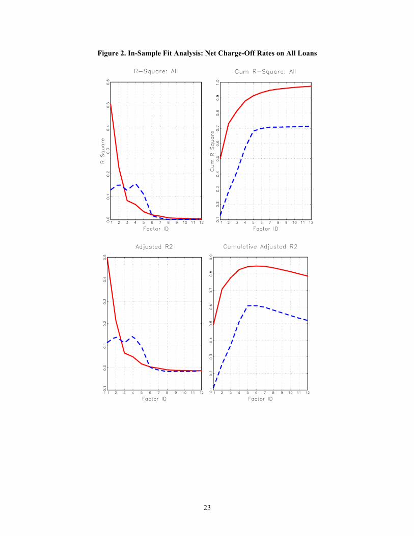
In Figure 2, we plot both the and adjusted obtained from least squares regressions of the
target variable on the estimated PLS factors (red line) and PC factors (blue line) for up to 12
factors ( 12) as well as their cumulative for the charge-off rates on all loans for all banks.
Note that the factors are orthogonal to each other, thus the cumulative or cumulative adjusted
indicate how much variation of the net charge-off rates is explained by the bank-specific and
macroeconomic variables jointly. It should be also noted that PLS models outperform one of the
popularly used alternative models based on a principal component (PC) analysis (e.g., see Stock
and Watson, 2002). That is, PLS factors provide much better in-sample fit performance than PC
factors. For example, the from PLS factors (R=1) exceeds 0.5, whereas that from PC factors
(R=1) slightly exceeds 0.1 for the net charge-off rate for all loans. Given ∆ is estimated using
the covariance between the target and the predictor variables, this result is not surprising as well
as the finding that the adjusted plot shows almost identical in-sample fit as that of the .
One notable point to be made is that unlike the PLS factors, the contribution of the PC
factors do not necessarily diminish when the number of factors increases. This is because the PC

16
factors are estimated solely from the variance-covariance matrix of the predictor variables, while
the PLS factors are formulated to obtain the most predictive content of the target variable from the
predictors. Note that the from the PC factors is the highest for the fourth factor estimate,
whereas the contribution of the PLS factors to are the highest for the first factor estimate. That
is, the marginal decreases when we regress the net charge-off rates on subsequent PLS factors.
In contrast, the PC approach considers covariance within the predictors, so that the marginal
does not necessarily decrease as the number of factors increases.
Figure 2 around here
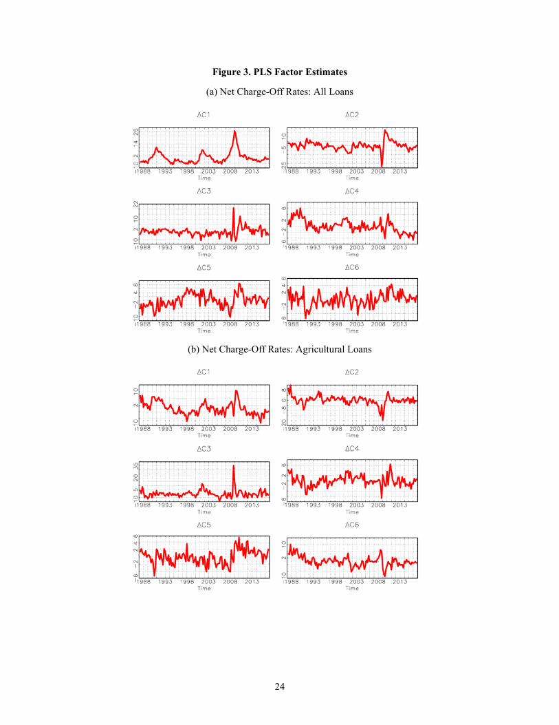
Figure 3 reports estimated PLS factors, ∆ , for up to 6 factors in panel (a) for all bank
charge-off rates on all loans and in panel (b) for all bank charge-off rates on agricultural loans,
respectively. As can be seen in Figure 1, agricultural loans show a high degree of heterogeneity in
comparison with other types of charge-off rates. It should be noted that the PLS factors of all loans
are quite different from those of agricultural loans. Such distinct factor estimates form the PLS
implies that the performance for all bank charge-off rates on all loans and for all bank charge-off
rates on agricultural loans will differ in the out-of-sample forecasting exercises we report in next
section.
Furthermore, Figure 4 shows their associated factor loading coefficient estimates. These
two series show very different estimated PLS weighting matrices. For example, Group 1 (National
Income and Product Account by the BEA) and Group 3 (Employment and Unemployment)
contribute more to the first PLS factor estimate for the all bank charge-off rates on all loans, while
Group 6 (Prices) contributes more to that for all bank charge-off rates on agricultural loans. The
weights on other predictor variables for the other five PLS factor estimates show substantial
heterogeneity across all 14 categorized predictor groups. However, since we are mainly interested

17
in the out-of-sample forecasting performance of the PLS model compared to other competing
models, we do not attempt to trace individual bank-specific and macroeconomic variables
incorporated in these factors.
Figures 3 and 4 around here
4.2. Forecasting Charge-Off Rates
4.2.1. All Bank Charge-Off Rates
Out-of-sample predictability evaluations for the all banks charge-off rate on all loans are reported
in Figures 5 and 6 for the recursive and the rolling window scheme, respectively. We use % for
the sample split point, that is, the initial 50 percent of observations are used as a training set to
formulate the first out-of-sample forecast in implementing forecasting exercises via the recursive
scheme as well as the rolling window scheme. We report results with the PLSAR for up to 12
forecast horizons (3 years) with up to 12 estimated common factors. That is, we report 144
RRMSPE’s in each graph. Darker areas indicate the cases in which the PLSAR model outperforms
both benchmark models, RW and AR models.
In Figure 5, we use the recursive scheme to calculate RRMSPE of the PLSAR relative to
that of the RW or AR benchmark models. The PLSAR model overall dominates the two benchmark
models. When comparted to the AR benchmark model, however, the AR benchmark model
outperforms the PLSAR model over most horizons with a small number of factors. As the forecast
horizons and the number of factors employed in forecasting increase, the PLSAR model
outperforms the AR benchmark model.
In Figure 6, we implement the rolling window scheme to calculate RRMSPE of the PLSAR
relative to that of the RW and AR benchmark models. Similar to the results from the recursive
scheme, the PLSAR model outperforms the two benchmark models, especially when the number

18
of forecast horizons increases and when more factors are employed in forecasting. Of course, as
noted earlier, more factors are appropriate insofar as losses on loans are determined by many
variables, including both bank-specific and macroeconomic variables. However, the two
benchmark models provide more accurate forecasts over some horizons than the PLSAR model,
depending on the number of factors employed in forecasting. In particular, the RW and AR
benchmark models outperform the PLSAR model over most horizons with a small number of
factors. Similar to the findings from the recursive scheme, as the forecast horizons and the number
of factors employed in forecasting increases, the PLSAR model outperforms the RW and AR
benchmark models. Instead of the PLSAR model, when using the PLSRW as our suggested model,
we find similar results.
In summary, we do not find any advantages associated with using the rolling window
method as compared to the recursive method, since more observations help enhance the out-of-
sample predictability of the PLS factor forecasting models.
Figures 5 and 6 around here
4.2.2. Individual Bank Charge-Off Rates
In the previous section, we are able to determine which of the two forecast schemes, recursive or
rolling window, provides the better forecast of the net charge-off rates on all loans. As also noted,
since the recursive scheme helps enhance out-of-sample predictability of the PLS factor
forecasting models, we report our findings for the net charge-off rates on all loans of two big and
important banks, Bank of America and JPMorgan Chase, using the recursive forecast scheme.
The sample period covers 1991:Q1 to 2016:Q4. We obtain the net charge-off rates for the
two banks from the Consolidated Financial Statements for Bank Holding Companies (the FR Y-
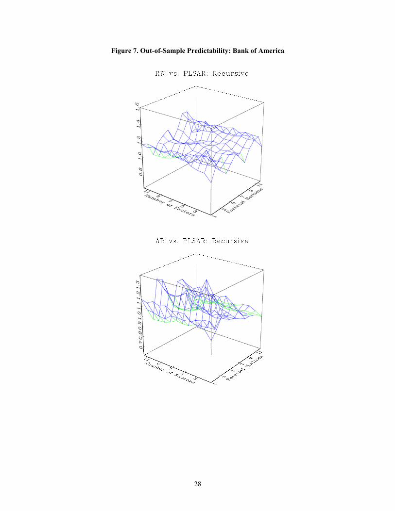
9C form) from the Federal Reserve Bank of Chicago website. Figure 7 shows similar out-of-

19
sample forecast results for the net charge-off rates on all loans for Bank of America. In general,
the PLSAR model outperforms the two benchmark models for most forecast horizons. However,
the two benchmark models provide better forecasting accuracy over some horizons than the
PLSAR model. In particular, the AR benchmark outperforms the PLSAR model over different
horizons more often compared to the RW benchmark.
Figures 7 around here
Figure 8 shows out-of-sample forecast results for the net charge-off rates on all loans for
JPMorgan Chase. Consistent with the previous results, the PLSAR model outperforms the two
benchmark models for most forecast horizons. For this bank, the PLSAR dominates the RW
benchmark model no matter how many forecast horizons are used and the number of factors
employed in forecasting. However, the AR benchmark model still provides a more accurate
forecast over some horizons than the PLSAR model when the number of factors employed in
forecasting is relatively small, which has the downside of omitting important variables that
influence losses on loans. Unlike out-of-sample predictability evaluations for the all banks charge-
off rates on all loans, we do not find a similar pattern for the two individual banks. In other words,
as the forecast horizons and the number of factors employed in forecasting increase, the PLSAR
model outperforms the RW and AR benchmark models.
Figures 8 around here
5. Conclusions
We have evaluated the forecasting accuracy of a partial least squares (PLS) model as
compared to two simpler benchmark models because it allows one to include more predictor
variables than observations in forecasting bank losses, or net charge-offs. This is important insofar
as there are generally far more variables that can affect the net charge-off rates of banks than the

20
number of available observations in any forecasting exercise. We therefore used a PLS model to
obtain forecasts for net charge-off rates for all banks and two very big banks based on more than
two hundred predictor variables for the period1991:Q1 to 2016:Q4.
Based on both a rolling window scheme and a recursive scheme, we find that the PLSAR
model outperforms the two benchmark models for forecasting the net charge-off rate for all banks,
especially when the number of forecast horizons increases and when more factors are employed
in forecasting. In general, the PLSAR model outperforms the benchmark models for most forecast
horizons in the case of the net charge-off rate on all loans for Bank of America. When forecasting
the net charge-off rates on all loans for JPMorgan Chase, we also find that the PLSAR model
outperforms the benchmark models for most forecast horizons. Moreover, for this bank, the
PLSAR dominates the RW benchmark model no matter how many forecast horizons are used and
the number of factors employed in forecasting.
In summary, given the importance of forecasting a variety of bank variables, including net
charge-offs, that are affected by numerous factors, the PLS model has the key advantage that it
does not constrain the number of predictors to be less than the number of observations in a
forecasting exercise. This is important reason to make future use of such a model in forecasting a
wider range of target variables than simply net charge-off rates.

21
Figure 1. Net Charge-Off Rates

22
Table 1. Macroeconomic Data Classification
23
Figure 2. In-Sample Fit Analysis: Net Charge-Off Rates on All Loans
24
Figure 3. PLS Factor Estimates
(a) Net Charge-Off Rates: All Loans
(b) Net Charge-Off Rates: Agricultural Loans

25
Figure 4. PLS Weighting Matrix Estimates
(a) Net Charge-Off Rates: All Loans
(b) Net Charge-Off Rates: Agricultural Loans

26
Figure 5. Out-of-Sample Predictability: Recursive Scheme for the PLSAR Model

27
Figure 6. Out-of-Sample Predictability: Rolling-Window Scheme for the PLSAR Model
28
Figure 7. Out-of-Sample Predictability: Bank of America

29
Figure 8. Out-of-Sample Predictability: Chase

30
References
Andersson, M. (2009). A comparison of nine PLS1 algorithms. Journal of Chemometrics, 23(10), 518-529.
Arnett, D. B., Laverie, D. A., & Meiers, A. (2003). Developing parsimonious retailer equity indexes using partial least squares analysis: a method and applications. Journal of Retailing, 79(3), 161-170.
Avkiran, N. K. (2018). Rise of the partial least squares structural equation modeling: An application in banking. In: Avkiran N., Ringle C. (eds) Partial Least Squares Structural Equation Modeling (pp. 1-29). International Series in Operations Research & Management Science, vol 267. Springer, Cham.
Avkiran, N. K., Ringle, C., & Low, R. (Forthcoming). Monitoring transmission of systemic risk: Application of PLS-SEM in financial stress testing. The Journal of Risk.
Ayadurai, C., & Eskandari, R. (2018). Bank soundness: a PLS-SEM approach. In: Avkiran N., Ringle C. (eds) Partial Least Squares Structural Equation Modeling (pp. 31-52). International Series in Operations Research & Management Science, vol 267. Springer, Cham.
Bontis, N., Booker, L. D., & Serenko, A. (2007). The mediating effect of organizational reputation on customer loyalty and service recommendation in the banking industry. Management Decision, 45(9), 1426-1445.
Cochrane, J. H., (2008). The dog that did not bark: A defense of return predictability. The Review of Financial Studies, 21(4), 1533-1575.
Goh, C., Ali, M., & Rasli, A. (2014). The use of partial least squares path modeling in causal inference for archival financial accounting research. Jurnal Teknologi, 68(3), 57-62.
Helland, I. S. (1990). Partial least squares regression and statistical models. Scandinavian Journal of Statistics, 97-114.
Huang, D., Jiang, F., Tu, J., & Zhou, G. (2015). Investor sentiment aligned: A powerful predictor of stock returns. The Review of Financial Studies, 28(3), 791-837.
Kelly, B., & Pruitt, S. (2013). Market expectations in the cross‐section of present values. The Journal of Finance, 68(5), 1721-1756.
Kim, H., & Ko, K. (2017). Improving forecast accuracy of financial vulnerability: partial least squares factor model approach. Bank of Korean Working Paper, 1-32.
Laitinen, E. K. (2006). Partial least squares regression in payment default prediction. Investment Management and Financial Innovations, 3(1), 64-77.
Larson, R. K., & Kenny, S. Y. (1995). An empirical analysis of international accounting standards, equity markets, and economic growth in developing countries. Journal of International Financial Management & Accounting, 6(2), 130-157.
Lee, L., Petter, S., Fayard, D., & Robinson, S. (2011). On the use of partial least squares path modeling in accounting research. International Journal of Accounting Information Systems, 12(4), 305-328.
Lie, E., Meng, B., Qian, Y., & Zhou, G. (2017). Corporate Activities and the Market Risk Premium. Nitzl, C. (2016). The use of partial least squares structural equation modelling (PLS-SEM) in
management accounting research: Directions for future theory development. Journal of Accounting Literature, 37, 19-35.

31
Poolthong, Y., & Mandhachitara, R. (2009). Customer expectations of CSR, perceived service quality and brand effect in Thai retail banking. International Journal of Bank Marketing, 27(6), 408-427.
Stock, J. H., & Watson, M. W. (2002). Forecasting using principal components from a large number of predictors. Journal of the American statistical association, 97(460), 1167-1179.

32
Appendix
Group 1: NIPA
id
description
1 Real Gross Domestic Product, 3 Decimal (Billions of Chained 2009 Dollars) 2 Real Personal Consumption Expenditures (Billions of Chained 2009
ll )3 Real Personal Consumption expenditures: Durable goods (Billions of h i d 2009 Dollars), deflated using PCE
4 Real Personal Consumption Expenditures: Services (Billions of 2009 ll ) deflated using PCE
5 Real Personal Consumption Expenditures: Nondurable Goods (Billions of Dollars), deflated using PCE
6 Real Gross Private Domestic Investment, 3 decimal (Billions of Chained Dollars)
7 Real private fixed investment (Billions of Chained 2009 Dollars), deflated using PCE
8 Real Gross Private Domestic Investment: Fixed Investment: Nonresidential: Equipment (Billions of Chained 2009 Dollars), deflated using PCE
9 Real private fixed investment: Nonresidential (Billions of Chained 2009 Dollars), deflated using PCE
10 Real private fixed investment: Residential (Billions of Chained 2009 ll ) deflated using PCE
11 Shares of gross domestic product: Gross private domestic investment: h in private inventories (Percent)
12 Real Government Consumption Expenditures & Gross Investment (Billions f Chained 2009 Dollars)
13 Real Government Consumption Expenditures and Gross Investment: d l (Percent Change from Preceding Period)
14 Real Federal Government Current Receipts (Billions of Chained 2009 ll ) deflated using PCE
15 Real government state and local consumption expenditures (Billions of Chained 2009 Dollars), deflated using PCE
16 Real Exports of Goods & Services, 3 Decimal (Billions of Chained 2009 Dollars)
17 Real Imports of Goods & Services, 3 Decimal (Billions of Chained 2009 Dollars)
18 Real Disposable Personal Income (Billions of Chained 2009 Dollars) 19 Nonfarm Business Sector: Real Output (Index 2009=100)20 Business Sector: Real Output (Index 2009=100)21 Manufacturing Sector: Real Output (Index 2009=100)194 Shares of gross domestic product: Exports of goods and services (Percent) 195 Shares of gross domestic product: Imports of goods and services (Percent)

33
Group 2: Industrial Production
id description
22 Industrial Index (Index 2012=100) 23 Industrial
d iFinal Products (Market Group) (Index 2012=100)
24 Industrial d i
Consumer Goods (Index 2012=100) 25 Industrial
d iMaterials (Index 2012=100)
26 Industrial d i
Durable Materials (Index 2012=100) 27 Industrial
d iNondurable Materials (Index 2012=100)
28 Industrial d i
Durable Consumer Goods (Index 2012=100) 29 Industrial
d iDurable Goods: Automotive products (Index
)30 Industrial d i
Nondurable Consumer Goods (Index 2012=100) 31 Industrial
d iBusiness Equipment (Index 2012=100)
32 Industrial d i
Consumer energy products (Index 2012=100) 33 Capacity Utilization: Total Industry (Percent of Capacity) 34 Capacity Utilization: Manufacturing (SIC) (Percent of Capacity) 198 Industrial Production: Manufacturing (SIC) (Index 2012=100) 199 Industrial Production: Residential Utilities (Index 2012=100) 200 Industrial Production: Fuels (Index 2012=100) 201 ISM Manufacturing: Production Index 205 ISM Manufacturing: PMI Composite Index

34
Group 3: Employment and Unemployment
id
description
35 All Employees: Total nonfarm (Thousands of Persons)36 All Employees: Total Private Industries (Thousands of Persons)37 All Employees: Manufacturing (Thousands of Persons)38 All Employees: Service-Providing Industries (Thousands of Persons) 39 All Employees: Goods-Producing Industries (Thousands of Persons) 40 All Employees: Durable goods (Thousands of Persons)41 All Employees: Nondurable goods (Thousands of Persons)42 All Employees: Construction (Thousands of Persons)43 All Employees: Education & Health Services (Thousands of Persons) 44 All Employees: Financial Activities (Thousands of Persons)45 All Employees: Information Services (Thousands of Persons)46 All Employees: Professional & Business Services (Thousands of Persons) 47 All Employees: Leisure & Hospitality (Thousands of Persons)48 All Employees: Other Services (Thousands of Persons)49 All Employees: Mining and logging (Thousands of Persons)50 All Employees: Trade, Transportation & Utilities (Thousands of Persons) 51 All Employees: Government (Thousands of Persons)52 All Employees: Retail Trade (Thousands of Persons)53 All Employees: Wholesale Trade (Thousands of Persons)54 All Employees: Government: Federal (Thousands of Persons)55 All Employees: Government: State Government (Thousands of Persons) 56 All Employees: Government: Local Government (Thousands of Persons) 57 Civilian Employment (Thousands of Persons)58 Civilian Labor Force Participation Rate (Percent)59 Civilian Unemployment Rate (Percent)60 Unemployment Rate less than 27 weeks (Percent)61 Unemployment Rate for more than 27 weeks (Percent)62 Unemployment Rate - 16 to 19 years (Percent)63 Unemployment Rate - 20 years and over, Men (Percent)64 Unemployment Rate - 20 years and over, Women (Percent)65 Number of Civilians Unemployed - Less Than 5 Weeks (Thousands of
)66 Number of Civilians Unemployed for 5 to 14 Weeks (Thousands of Persons) 67 Number of Civilians Unemployed for 15 to 26 Weeks (Thousands of Persons) 68 Number of Civilians Unemployed for 27 Weeks and Over (Thousands of
)69 Unemployment Level - Job Losers (Thousands of Persons)70 Unemployment Level - Reentrants to Labor Force (Thousands of Persons) 71 Unemployment Level - Job Leavers (Thousands of Persons)72 Unemployment Level - New Entrants (Thousands of Persons)

35
Group 3: Employment and Unemployment, continued
id
description
73 Employment Level - Part-Time for Economic Reasons, All Industries (Thousands of Persons)
74 Business Sector: Hours of All Persons (Index 2009=100)75 Manufacturing Sector: Hours of All Persons (Index 2009=100)76 Nonfarm Business Sector: Hours of All Persons (Index 2009=100)77 Average Weekly Hours of Production and Nonsupervisory Employees:
f i (Hours) 78 Average Weekly Hours Of Production And Nonsupervisory Employees: Total private
(Hours) 79 Average Weekly Overtime Hours of Production and Nonsupervisory Employees:
Manufacturing (Hours) 80 Help-Wanted Index 202 Average (Mean) Duration of Unemployment (Weeks)203 Average Weekly Hours of Production and Nonsupervisory Employees: Goods-
d i204 ISM Manufacturing: Employment Index229 Ratio of Help Wanted/No. Unemployed230 Initial Claims
Group 4: Housing
id
description
81 Housing Starts: Total: New Privately Owned Housing Units Started Units)
82 Privately Owned Housing Starts: 5-Unit Structures or More (Thousands of i )83 New Private Housing Units Authorized by Building Permits (Thousands of i )84 Housing Starts in Midwest Census Region (Thousands of Units)
85 Housing Starts in Northeast Census Region (Thousands of Units)86 Housing Starts in South Census Region (Thousands of Units)87 Housing Starts in West Census Region (Thousands of Units)183 All-Transactions House Price Index for the United States (Index 1980 Q1=100) 184 S&P/Case-Shiller 10-City Composite Home Price Index (Index January 2000 =
100) 185 S&P/Case-Shiller 20-City Composite Home Price Index (Index January 2000 =
100) 236 New Private Housing Units Authorized by Building Permits in the Northeast
Census Region (Thousands, SAAR)237 New Private Housing Units Authorized by Building Permits in the Midwest
Census Region (Thousands, SAAR)238 New Private Housing Units Authorized by Building Permits in the South
Region (Thousands, SAAR)239 New Private Housing Units Authorized by Building Permits in the West Census
Region (Thousands, SAAR)

36
Group 5: Inventories, Orders, and Sales
id
description
88 Real Manufacturing and Trade Industries Sales (Millions of Chained 2009 Dollars)
89 Real Retail and Food Services Sales (Millions of Chained 2009 Dollars), d fl d by Core PCE
90 Real Manufacturers’ New Orders: Durable Goods (Millions of 2009 Dollars), deflated by Core PCE
91 Real Value of Manufacturers’ New Orders for Consumer Goods Industries (Million of 2009 Dollars), deflated by Core PCE
92 Real Value of Manufacturers’ Unfilled Orders for Durable Goods Industries (Million of 2009 Dollars), deflated by Core PCE
93 Real Value of Manufacturers’ New Orders for Capital Goods: Nondefense Capital Goods Industries (Million of 2009 Dollars), deflated by Core PCE
94 ISM Manufacturing: Supplier Deliveries Index (lin)95 Real Manufacturing and Trade Inventories (Millions of 2009 Dollars) 206 ISM Manufacturing: New Orders Index207 ISM Manufacturing: Inventories Index231 Total Business Inventories (Millions of Dollars)232 Total Business: Inventories to Sales Ratio

37
Group 6: Prices
id
description
96 Personal Consumption Expenditures: Chain-type Price Index (Index 2009=100)
97 Personal Consumption Expenditures Excluding Food and Energy (Chain-Type Price Index) (Index 2009=100)
98 Gross Domestic Product: Chain-type Price Index (Index 2009=100) 99 Gross Private Domestic Investment: Chain-type Price Index (Index
2009=100) 100 Business Sector: Implicit Price Deflator (Index 2009=100) 101 Personal consumption expenditures: Goods (chain-type price index) 102 Personal consumption expenditures: Durable goods (chain-type price
index) 103 Personal consumption expenditures: Services (chain-type price index) 104 Personal consumption expenditures: Nondurable goods (chain-type
index) 105 Personal consumption expenditures: Services: Household consumption
expenditures (chain-type price index) 106 Personal consumption expenditures: Durable goods: Motor vehicles
parts (chain-type price index) 107 Personal consumption expenditures: Durable goods: Furnishings and
durable household equipment (chain-type price index) 108 Personal consumption expenditures: Durable goods: Recreational
and vehicles (chain-type price index) 109 Personal consumption expenditures: Durable goods: Other durable
(chain-type price index) 110 Personal consumption expenditures: Nondurable goods: Food and
beverages purchased for off-premises consumption (chain-type price index) 111 Personal consumption expenditures: Nondurable goods: Clothing and
footwear (chain-type price index) 112 Personal consumption expenditures: Nondurable goods: Gasoline and
other energy goods (chain-type price index) 113 Personal consumption expenditures: Nondurable goods: Other
nondurable goods (chain-type price index) 114 Personal consumption expenditures: Services: Housing and utilities
(chain-type price index) 115 Personal consumption expenditures: Services: Health care (chain-type
price index) 116 Personal consumption expenditures: Transportation services (chain-
price index)

38
Group 6: Prices, continued
id
description
117 Personal consumption expenditures: Recreation services (chain-type price index) 118 Personal consumption expenditures: Services: Food services and
accommodations (chain-type price index)119 Personal consumption expenditures: Financial services and insurance
(chain-type price index)120 Personal consumption expenditures: Other services (chain-type price
index) 121 Consumer Price Index for All Urban Consumers: All Items (Index
1982-84=100) 122 Consumer Price Index for All Urban Consumers: All Items Less Food &
Energy (Index 1982-84=100)123 Producer Price Index by Commodity for Finished Goods (Index
)124 Producer Price Index for All Commodities (Index 1982=100)125 Producer Price Index by Commodity for Finished Consumer Goods
( d 1982=100) 126 Producer Price Index by Commodity for Finished Consumer Foods
( d 1982=100) 127 Producer Price Index by Commodity Industrial Commodities (Index
1982=100) 128 Producer Price Index by Commodity Intermediate Materials: Supplies &
Components (Index 1982=100)129 ISM Manufacturing: Prices Index (Index)130 Producer Price Index by Commodity for Fuels and Related Products
d Power: Natural Gas (Index 1982=100)131 Producer Price Index by Commodity for Fuels and Related Products
d Power: Crude Petroleum (Domestic Production) (Index 1982=100) 132 Real Crude Oil Prices: West Texas Intermediate (WTI) - Cushing,
Oklahoma (2009 Dollars per Barrel), deflated by Core PCE214 Producer Price Index: Crude Materials for Further Processing (Index
1982=100) 215 Producer Price Index: Commodities: Metals and metal products:
i nonferrous metals (Index 1982=100)216 Consumer Price Index for All Urban Consumers: Apparel (Index
1982-84=100) 217 Consumer Price Index for All Urban Consumers: Transportation (Index
1982-84=100) 218 Consumer Price Index for All Urban Consumers: Medical Care (Index
1982-84=100) 219 Consumer Price Index for All Urban Consumers: Commodities (Index
1982-84=100) 220 Consumer Price Index for All Urban Consumers: Durables (Index
1982-84=100) 221 Consumer Price Index for All Urban Consumers: Services (Index
1982-84=100) 222 Consumer Price Index for All Urban Consumers: All Items Less Food
(Index 1982-84=100)223 Consumer Price Index for All Urban Consumers: All items less shelter
(Index 1982-84=100)224 Consumer Price Index for All Urban Consumers: All items less medical
care (Index 1982-84=100)242 CPI for All Urban Consumers: Owners’ equivalent rent of residences
(Index Dec 1982=100)

39
Group 7: Earnings and Productivity
id
description
133 Real Average Hourly Earnings of Production and Nonsupervisory Employees: Private (2009 Dollars per Hour), deflated by Core PCE134 Real Average Hourly Earnings of Production and Nonsupervisory Employees:
Construction (2009 Dollars per Hour), deflated by Core PCE135 Real Average Hourly Earnings of Production and Nonsupervisory Employees:
Manufacturing (2009 Dollars per Hour), deflated by Core PCE136 Manufacturing Sector: Real Compensation Per Hour (Index 2009=100) 137 Nonfarm Business Sector: Real Compensation Per Hour (Index 2009=100) 138 Business Sector: Real Compensation Per Hour (Index 2009=100)139 Manufacturing Sector: Real Output Per Hour of All Persons (Index 2009=100) 140 Nonfarm Business Sector: Real Output Per Hour of All Persons (Index
)141 Business Sector: Real Output Per Hour of All Persons (Index 2009=100) 142 Business Sector: Unit Labor Cost (Index 2009=100)143 Manufacturing Sector: Unit Labor Cost (Index 2009=100)144 Nonfarm Business Sector: Unit Labor Cost (Index 2009=100)145 Nonfarm Business Sector: Unit Nonlabor Payments (Index 2009=100) 225 Average Hourly Earnings of Production and Nonsupervisory Employees:
Goods-Producing (Dollars per Hour)
Group 8: Interest Rates
id
description
146 Effective Federal Funds Rate (Percent)147 3-Month Treasury Bill: Secondary Market Rate (Percent)148 6-Month Treasury Bill: Secondary Market Rate (Percent)149 3-Month Eurodollar Deposit Rate (London) (Percent)150 1-Year Treasury Constant Maturity Rate (Percent)151 10-Year Treasury Constant Maturity Rate (Percent)152 30-Year Conventional Mortgage Rate (Percent)153 Moody’s Seasoned Aaa Corporate Bond Yield (Percent)154 Moody’s Seasoned Baa Corporate Bond Yield (Percent)155 Moody’s Seasoned Baa Corporate Bond Yield Relative to Yield on 10-Year Treasury
Constant Maturity (Percent)156 30-Year Conventional Mortgage Rate Relative to 10-Year Treasury Constant
i (Percent) 157 6-Month Treasury Bill Minus 3-Month Treasury Bill, secondary market (Percent) 158 1-Year Treasury Constant Maturity Minus 3-Month Treasury Bill, secondary
k (Percent) 159 10-Year Treasury Constant Maturity Minus 3-Month Treasury Bill, secondary
k (Percent) 160 3-Month Commercial Paper Minus 3-Month Treasury Bill, secondary market
( )161 3-Month Eurodollar Deposit Minus 3-Month Treasury Bill, secondary market ( )210 5-Year Treasury Constant Maturity Rate
211 3-Month Treasury Constant Maturity Minus Federal Funds Rate212 5-Year Treasury Constant Maturity Minus Federal Funds Rate213 Moody’s Seasoned Aaa Corporate Bond Minus Federal Funds Rate234 3-Month AA Financial Commercial Paper Rate235 3-Month Commercial Paper Minus Federal Funds Rate

40
Group 9: Money and Credit
id
description
162 St. Louis Adjusted Monetary Base (Billions of 1982-84 Dollars), deflated by 163 Real Institutional Money Funds (Billions of 2009 Dollars), deflated by Core 164 Real M1 Money Stock (Billions of 1982-84 Dollars), deflated by CPI 165 Real M2 Money Stock (Billions of 1982-84 Dollars), deflated by CPI 166 Real MZM Money Stock (Billions of 1982-84 Dollars), deflated by CPI 167 Real Commercial and Industrial Loans, All Commercial Banks (Billions of
U.S. Dollars), deflated by Core PCE168 Real Consumer Loans at All Commercial Banks (Billions of 2009 U.S.
ll ) deflated by Core PCE169 Total Real Nonrevolving Credit Owned and Securitized, Outstanding (Billions
f Dollars), deflated by Core PCE170 Real Real Estate Loans, All Commercial Banks (Billions of 2009 U.S.
ll ) deflated by Core PCE171 Total Real Revolving Credit Owned and Securitized, Outstanding (Billions of
2009 Dollars), deflated by Core PCE172 Total Consumer Credit Outstanding, deflated by Core PCE173 FRB Senior Loans Officer Opions. Net Percentage of Domestic Respondents
Reporting Increased Willingness to Make Consumer Installment Loans 208 Total Reserves of Depository Institutions (Billions of Dollars)209 Reserves Of Depository Institutions, Nonborrowed (Millions of Dollars) 226 Consumer Motor Vehicle Loans Outstanding Owned by Finance Companies
(Millions of Dollars) 227 Total Consumer Loans and Leases Outstanding Owned and Securitized by
Finance Companies (Millions of Dollars)228 Securities in Bank Credit at All Commercial Banks (Billions of Dollars)
Group 10: Household Balance Sheets
id
description
174 Real Total Assets of Households and Nonprofit Organizations (Billions of 2009 Dollars), deflated by Core PCE175 Real Total Liabilities of Households and Nonprofit Organizations (Billions of
Dollars), deflated by Core PCE176 Liabilities of Households and Nonprofit Organizations Relative to Personal
Disposable Income (Percent)177 Real Net Worth of Households and Nonprofit Organizations (Billions of 2009
Dollars), deflated by Core PCE178 Net Worth of Households and Nonprofit Organizations Relative to Disposable
Personal Income (Percent)179 Real Assets of Households and Nonprofit Organizations excluding Real Estate
Assets (Billions of 2009 Dollars), deflated by Core PCE180 Real Real Estate Assets of Households and Nonprofit Organizations (Billions
f 2009 Dollars), deflated by Core PCE181 Real Total Financial Assets of Households and Nonprofit Organizations
( illi of 2009 Dollars), deflated by Core PCE233 Nonrevolving consumer credit to Personal Income

41
Group 11: Exchange Rates
id
description
186 Trade Weighted U.S. Dollar Index: Major Currencies (Index March 187 U.S. / Euro Foreign ExchangeRate (U.S. Dollars to One Euro)188 Switzerland / U.S. ForeignExchangeRate189 Japan / U.S. Foreign Exchange Rate190 U.S. / U.K. Foreign ExchangeRate191 Canada / U.S. ForeignExchangeRate
Group 11: Exchange Rates
id
description
192 University of Michigan: Consumer Sentiment (Index 1st Quarter 1966=100) 193 Economic Policy Uncertainty Index for United States
Group 13: Stock Markets
id
description
182 CBOE S&P 100 Volatility Index: VXO240 Nikkei Stock Average241 NASDAQ Composite (Index Feb 5, 1971=100)254 S&P’s Common Stock Price Index: Composite255 S&P’s Common Stock Price Index: Industrials256 S&P’s Composite Common Stock: Dividend Yield257 S&P’s Composite Common Stock: Price-Earnings Ratio

42
Group 14: Non-Household Balance Sheets
id
description
196 Federal Debt: Total Public Debt as Percent of GDP (Percent)197 Real Federal Debt: Total Public Debt (Millions of 2009 Dollars), deflated by 243 Real Nonfinancial Corporate Business Sector Liabilities (Billions of 2009
ll ) Deflated by Implicit Price Deflator for Business Sector IPDBS244 Nonfinancial Corporate Business Sector Liabilities to Disposable Business
Income (Percent) 245 Real Nonfinancial Corporate Business Sector Assets (Billions of 2009 Dollars),
Deflated by Implicit Price Deflator for Business Sector IPDBS246 Real Nonfinancial Corporate Business Sector Net Worth (Billions of 2009
ll ) Deflated by Implicit Price Deflator for Business Sector IPDBS247 Nonfinancial Corporate Business Sector Net Worth to Disposable Business
(Percent) 248 Real Nonfinancial Noncorporate Business Sector Liabilities (Billions of 2009
Dollars), Deflated by Implicit Price Deflator for Business Sector IPDBS 249 Nonfinancial Noncorporate Business Sector Liabilities to Disposable Business
Income (Percent) 250 Real Nonfinancial Noncorporate Business Sector Assets (Billions of 2009
ll ) Deflated by Implicit Price Deflator for Business Sector IPDBS251 Real Nonfinancial Noncorporate Business Sector Net Worth (Billions of 2009
Dollars), Deflated by Implicit Price Deflator for Business Sector IPDBS 252 Nonfinancial Noncorporate Business Sector Net Worth to Disposable Business
Income (Percent) 253 Real Disposable Business Income, Billions of 2009 Dollars (Corporate cash flow
with IVA minus taxes on corporate income, deflated by Implicit Price Deflator f Business Sector IPDBS)