A criterion-based PLS approach to SEM

Michel Tenenhaus (HEC Paris)Arthur Tenenhaus (SUPELEC)

2

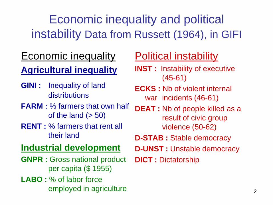
Economic inequality and political instability Data from Russett (1964), in GIFI

Economic inequalityAgricultural inequalityGINI : Inequality of land

distributionsFARM : % farmers that own half

of the land (> 50)RENT : % farmers that rent all

their land

Industrial developmentGNPR : Gross national product

per capita ($ 1955)LABO : % of labor force

employed in agriculture

Political instabilityINST : Instability of executive

(45-61)ECKS : Nb of violent internal

war incidents (46-61)DEAT : Nb of people killed as a

result of civic group violence (50-62)

D-STAB : Stable democracyD-UNST : Unstable democracy DICT : Dictatorship

3

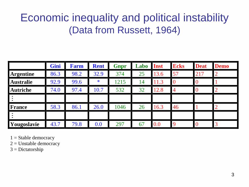
Economic inequality and political instability (Data from Russett, 1964)

Gini Farm Rent Gnpr Labo Inst Ecks Deat DemoArgentine 86.3 98.2 32.9 374 25 13.6 57 217 2Australie 92.9 99.6 * 1215 14 11.3 0 0 1Autriche 74.0 97.4 10.7 532 32 12.8 4 0 2

France 58.3 86.1 26.0 1046 26 16.3 46 1 2

Yougoslavie 43.7 79.8 0.0 297 67 0.0 9 0 3

1 = Stable democracy2 = Unstable democracy3 = Dictatorship

4

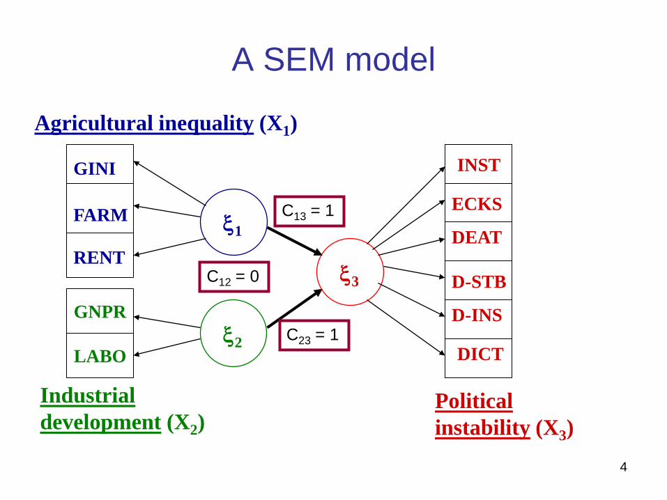
A SEM model

GINI

FARM

RENT

GNPR

LABO

Agricultural inequality (X1)

Industrialdevelopment (X2)

ECKS

DEAT

D-STB

D-INS

INST

DICT

Politicalinstability (X3)

ξ1

ξ2

ξ3

C13 = 1

C23 = 1

C12 = 0

5

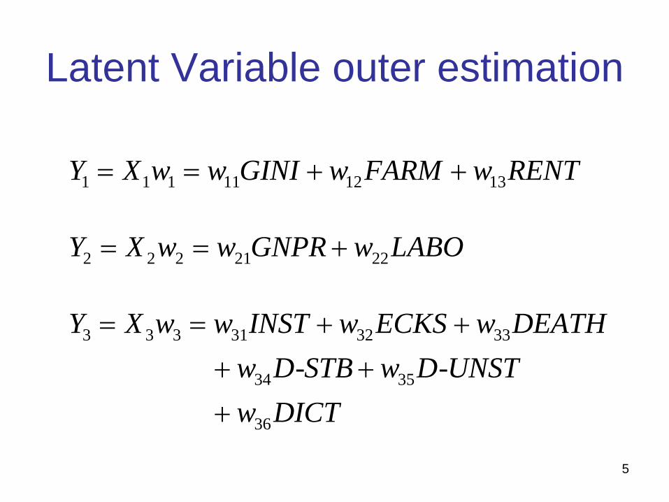
Latent Variable outer estimation

1 1 1 11 12 13Y X w w GINI w FARM w RENT= = + +

2 2 2 21 22Y X w w GNPR w LABO= = +

3 3 3 31 32 33

34 35

36

- -

Y X w w INST w ECKS w DEATHw D STB w D UNSTw DICT

= = + ++ ++

6

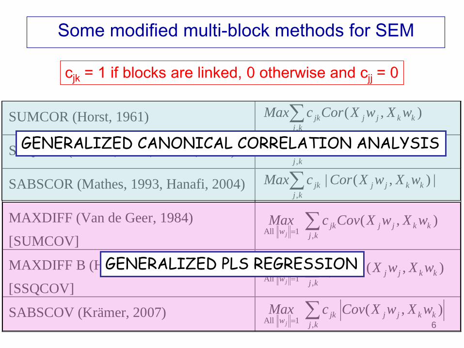
SUMCOR (Horst, 1961) ,

( , )jk j j k kj k

Max c Cor X w X w∑

SSQCOR (Mathes, 1993, Hanafi, 2004) 2

,( , )jk j j k k

j kMax c Cor X w X w∑

SABSCOR (Mathes, 1993, Hanafi, 2004) ,

| ( , ) |jk j j k kj k

Max c Cor X w X w∑

MAXDIFF (Van de Geer, 1984)

[SUMCOV] All 1 ,

( , )j

jk j j k kw j k

Max c Cov X w X w=∑

MAXDIFF B (Hanafi & Kiers, 2006)

[SSQCOV]

2

All 1 , ( , )

jjk j j k k

w j kMax c Cov X w X w

=∑

SABSCOV (Krämer, 2007) All 1 ,

( , )j

jk j j k kw j k

Max c Cov X w X w=∑

Some modified multi-block methods for SEM

cjk = 1 if blocks are linked, 0 otherwise and cjj = 0

GENERALIZED CANONICAL CORRELATION ANALYSIS

GENERALIZED PLS REGRESSION

7

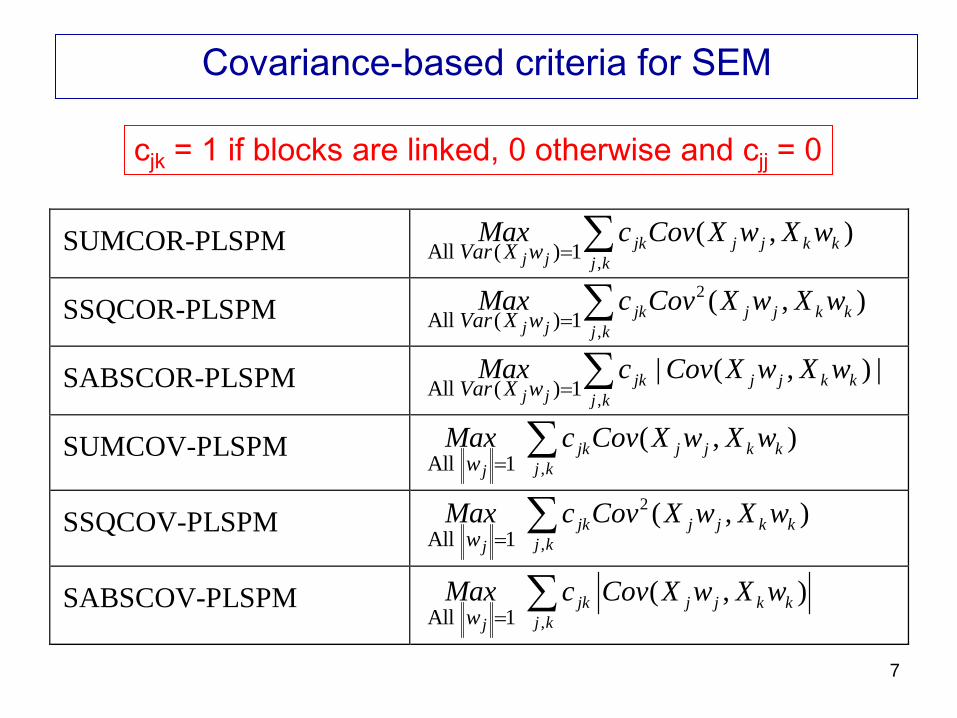
SUMCOR-PLSPM ,All ( ) 1

( , )jk j j k kj j j kVar X w

Max c Cov X w X w= ∑

SSQCOR-PLSPM 2

,All ( ) 1( , )jk j j k k

j j j kVar X wMax c Cov X w X w

= ∑

SABSCOR-PLSPM ,All ( ) 1

| ( , ) |jk j j k kj j j kVar X w

Max c Cov X w X w= ∑

SUMCOV-PLSPM ,All 1

( , )jk j j k kj kjw

Max c Cov X w X w=∑

SSQCOV-PLSPM 2

,All 1 ( , )jk j j k k

j kjwMax c Cov X w X w

=∑

SABSCOV-PLSPM ,All 1

( , )jk j j k kj kjw

Max c Cov X w X w=∑

Covariance-based criteria for SEM

cjk = 1 if blocks are linked, 0 otherwise and cjj = 0

8

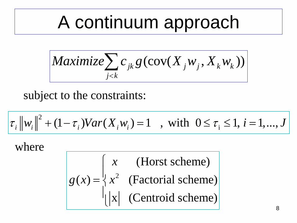
A continuum approach

(cov( , ))jk j j k kj k

Maximize c g X w X w<∑

subject to the constraints:

2i(1 ) ( ) 1 , with 0 1, 1,...,i i i i iw Var X w i Jτ τ τ+ − = ≤ ≤ =

where

2

(Horst scheme)( ) (Factorial scheme)

x (Centroid scheme)

xg x x

=

9

A general procedure to obtain critical points of the criteria

• Construct the Lagrangian function related to the optimization problem.

• Cancel the derivative of the Lagrangian function with respect to each wi.

• Use the Wold’s procedure to solve the stationary equations (≠ Lohmöller’s procedure).

• This procedure converges to a critical point of the criterion.

• The criterion increases at each step of the algorithm.

10

wjInitialstep Y2

Y1

YJ

Zj

ej1

ej2

ejJ

Innerestimation

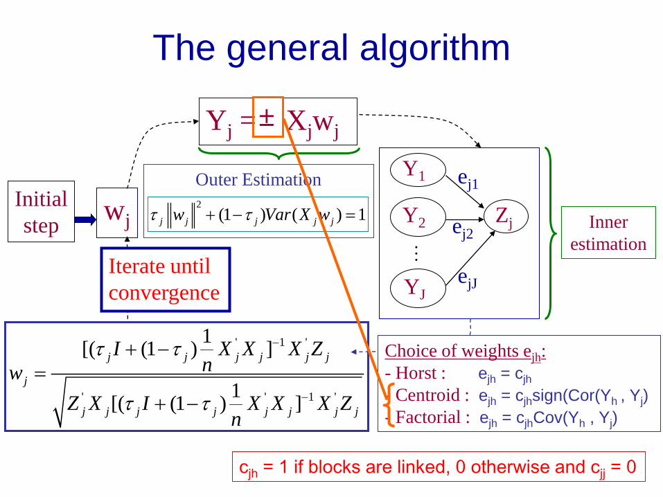
Yj = Xjwj

Outer Estimation2

(1 ) ( ) 1j j j j jw Var X wτ τ+ − =

The general algorithm

' 1 '

' ' 1 '

1[( (1 ) ]

1[( (1 ) ]

j j j j j j

j

j j j j j j j j

I X X X Znw

Z X I X X X Zn

τ τ

τ τ

−

−

+ −=

+ −

Choice of weights ejh:- Horst : ejh = cjh- Centroid : ejh = cjhsign(Cor(Yh , Yj) - Factorial : ejh = cjhCov(Yh , Yj)

cjh = 1 if blocks are linked, 0 otherwise and cjj = 0

±

Iterate untilconvergence

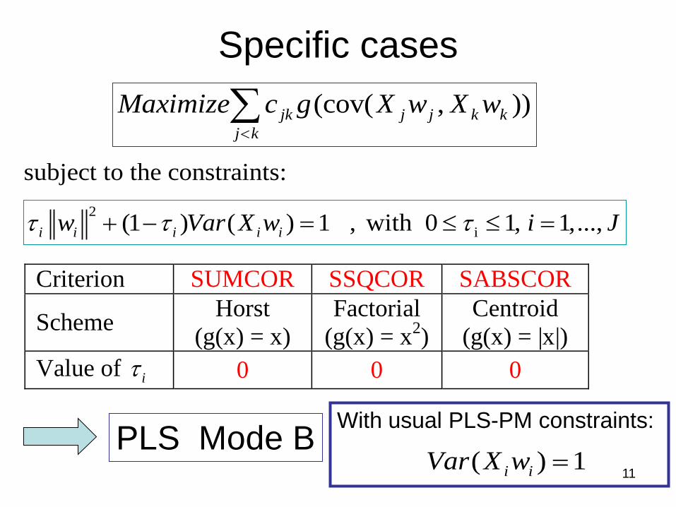
11

Specific cases(cov( , ))jk j j k k

j kMaximize c g X w X w

<∑

subject to the constraints:2

i(1 ) ( ) 1 , with 0 1, 1,...,i i i i iw Var X w i Jτ τ τ+ − = ≤ ≤ =

Criterion SUMCOR SSQCOR SABSCOR

Scheme Horst (g(x) = x)

Factorial (g(x) = x2)

Centroid (g(x) = |x|)

Value of iτ 0 0 0

PLS Mode B With usual PLS-PM constraints:

( ) 1i iVar X w =

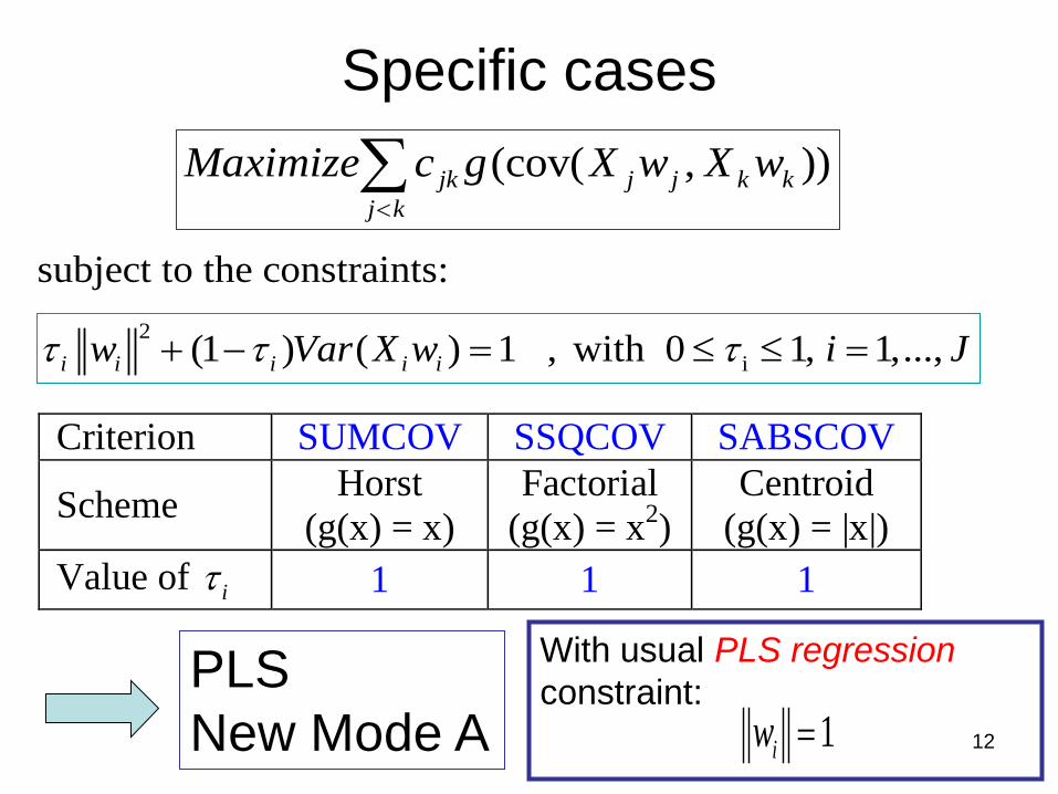
12

Specific cases(cov( , ))jk j j k k

j kMaximize c g X w X w

<∑

subject to the constraints:2

i(1 ) ( ) 1 , with 0 1, 1,...,i i i i iw Var X w i Jτ τ τ+ − = ≤ ≤ =

Criterion SUMCOV SSQCOV SABSCOV

Scheme Horst (g(x) = x)

Factorial (g(x) = x2)

Centroid (g(x) = |x|)

Value of iτ 1 1 1

PLSNew Mode A

With usual PLS regressionconstraint:

1iw =

13

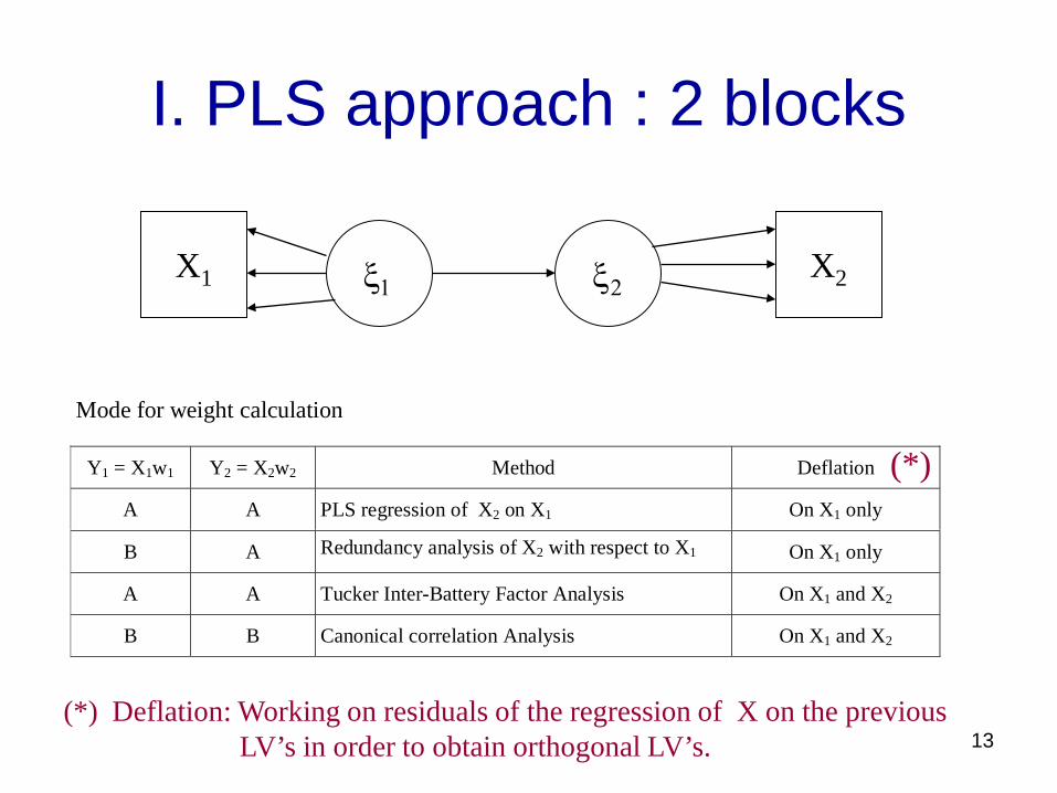
I. PLS approach : 2 blocks

X1 ξ1 ξ2 X2

Mode for weight calculation

Y1 = X1w1 Y2 = X2w2 Method Deflation

A A PLS regression of X2 on X1 On X1 only

B A Redundancy analysis of X2 with respect to X1 On X1 only

A A Tucker Inter-Battery Factor Analysis On X1 and X2

B B Canonical correlation Analysis On X1 and X2

(*)

(*) Deflation: Working on residuals of the regression of X on the previous LV’s in order to obtain orthogonal LV’s.

14

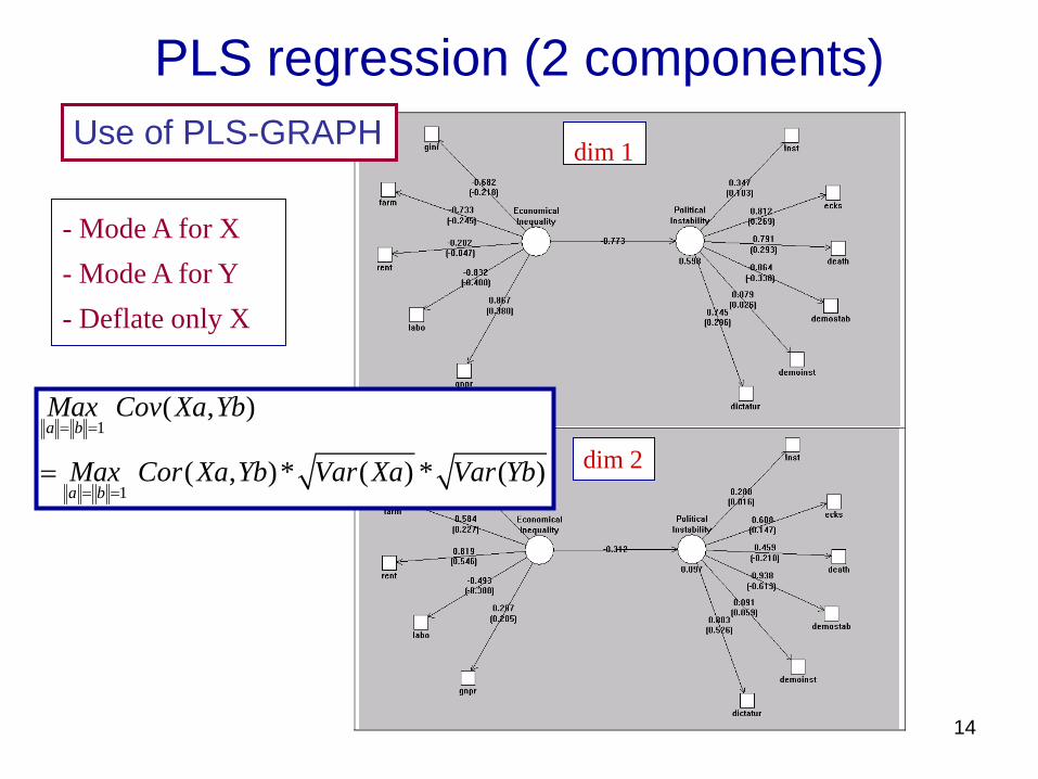
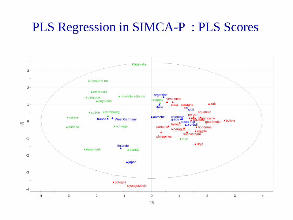
PLS regression (2 components)dim 1

dim 2

- Mode A for X- Mode A for Y- Deflate only X

1

1

( , )

( , )* ( ) * ( )

a b

a b

Max Cov Xa Yb

Max Cor Xa Yb Var Xa Var Yb

= =

= ==

Use of PLS-GRAPH

15

-4

-3

-2

-1

0

1

2

3

-4 -3 -2 -1 0 1 2 3 4

t[2]

t[1]

australie

belgique

canada

danemark

inde

irlande

luxembourg

pays-basnouvelle zélande

norvège

suèdesuisse

royaume-uni

états-unis

uruguay

autriche

brésil

japon

argentine

autriche

brésil

chili

colombiecosta-rica

finlande

france grèce

italie

japon

West Germany bolivie

cuba

rép. dominicaine

équateur

égypte

salvadorguatémalahonduras

irak

libye

nicaraguapanama

pèrou

philippines

pologne

sud vietnam

espagne

taiwan

venezuela

yougoslavie

PLS Regression in SIMCA-P : PLS Scores

16

-1.00

-0.80

-0.60

-0.40

-0.20

0.00

0.20

0.40

0.60

0.80

1.00

-1.00 -0.80 -0.60 -0.40 -0.20 0.00 0.20 0.40 0.60 0.80 1.00

pc(c

orr)[

Com

p. 2

]

pc(corr)[Comp. 1]

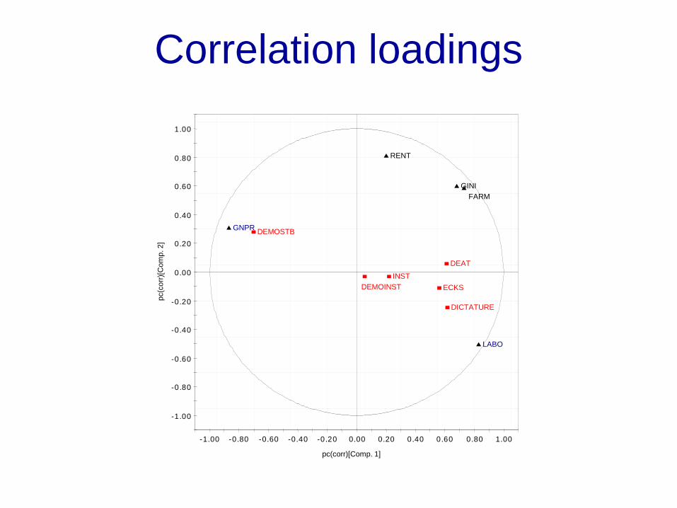
GINIFARM

RENT

GNPR

LABO

INSTECKS

DEAT

DEMOSTB

DEMOINST

DICTATURE

Correlation loadings

17

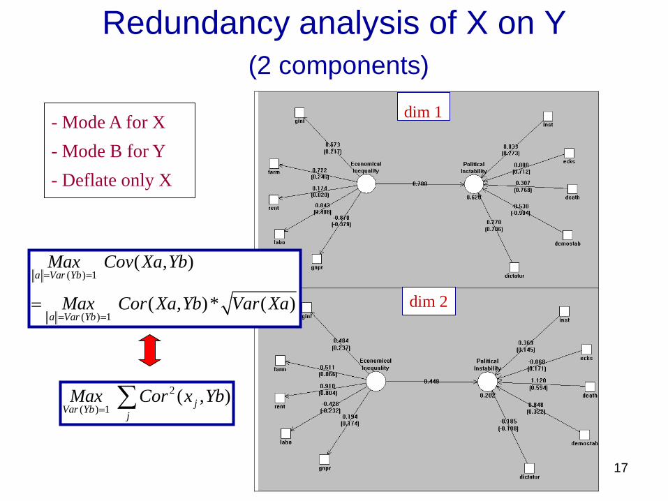
Redundancy analysis of X on Y(2 components)

- Mode A for X- Mode B for Y- Deflate only X

( ) 1

( ) 1

( , )

( , )* ( )

a Var Yb

a Var Yb

Max Cov Xa Yb

Max Cor Xa Yb Var Xa

= =

= ==

dim 1

dim 2

2

( ) 1 ( , )jVar Yb j

Max Cor x Yb=∑

18

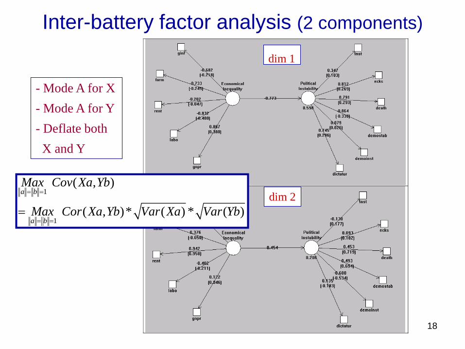
Inter-battery factor analysis (2 components)

dim 1

dim 2

- Mode A for X- Mode A for Y- Deflate bothX and Y

1

1

( , )

( , )* ( ) * ( )

a b

a b

Max Cov Xa Yb

Max Cor Xa Yb Var Xa Var Yb

= =

= ==

19

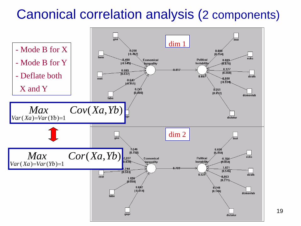
Canonical correlation analysis (2 components)

dim 1

dim 2

- Mode B for X- Mode B for Y- Deflate bothX and Y

( ) ( ) 1 ( , )

Var Xa Var YbMax Cov Xa Yb= =

( ) ( ) 1 ( , )

Var Xa Var YbMax Cor Xa Yb= =

20

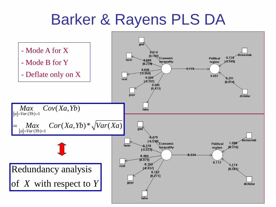
Barker & Rayens PLS DA

- Mode A for X- Mode B for Y- Deflate only on X

( ) 1

( ) 1

( , )

( , )* ( )

a Var Yb

a Var Yb

Max Cov Xa Yb

Max Cor Xa Yb Var Xa

= =

= ==

Redundancy analysisof with respect to X Y

21

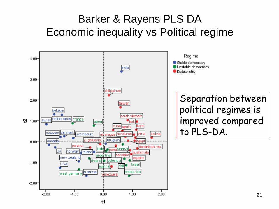
Barker & Rayens PLS DAEconomic inequality vs Political regime

Separation betweenpolitical regimes isimproved comparedto PLS-DA.

22

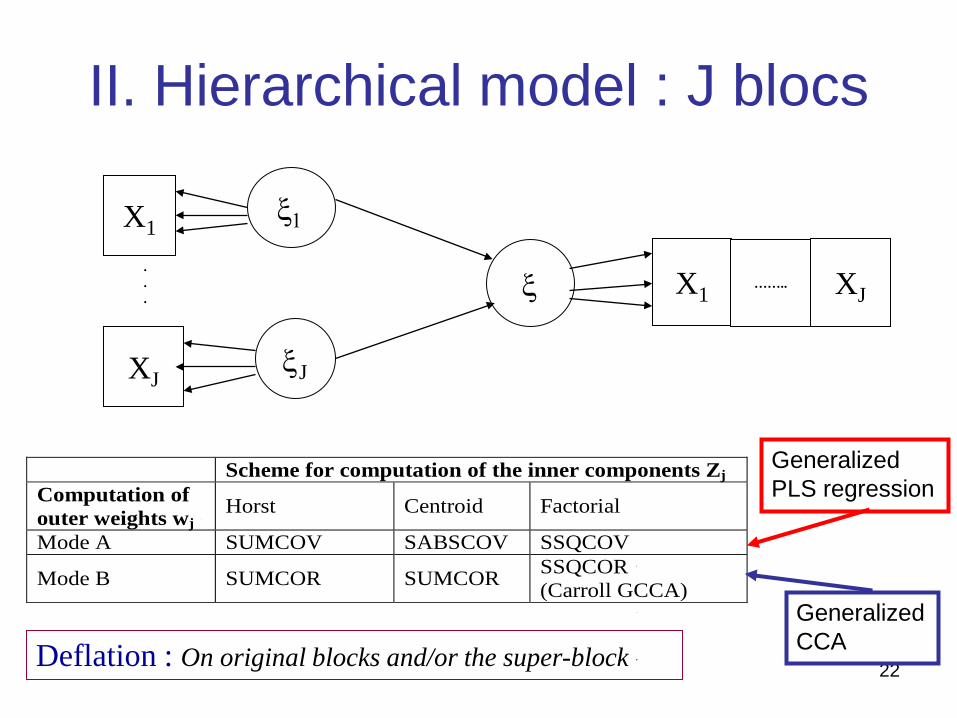
II. Hierarchical model : J blocs

X1

XJ

.

.

.

ξ1

ξJ

ξ X1 …….. XJ

Deflation : On original blocks and/or the super-block

Scheme for computation of the inner components Zj Computation of outer weights wj

Horst Centroid Factorial

Mode A SUMCOV SABSCOV SSQCOV

Mode B SUMCOR SUMCOR SSQCOR (Carroll GCCA)

GeneralizedPLS regression

GeneralizedCCA

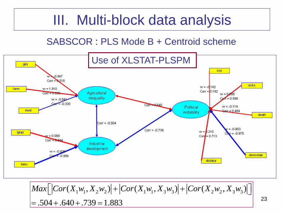
23

III. Multi-block data analysis SABSCOR : PLS Mode B + Centroid scheme

1 1 2 2 1 1 3 3 2 2 3 3( , ) ( , ) ( , )

.504 .640 .739 1.883

Max Cor X w X w Cor X w X w Cor X w X w + + = + + =

Use of XLSTAT-PLSPM

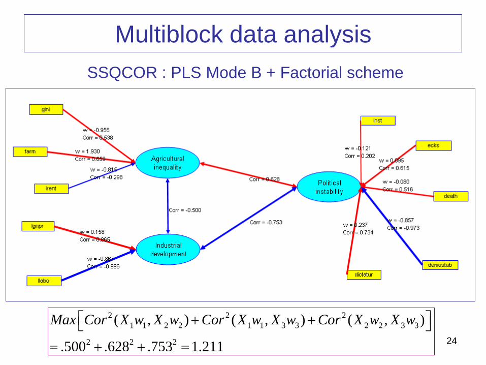
24

Multiblock data analysisSSQCOR : PLS Mode B + Factorial scheme

2 2 21 1 2 2 1 1 3 3 2 2 3 3

2 2 2

( , ) ( , ) ( , )

.500 .628 .753 1.211

Max Cor X w X w Cor X w X w Cor X w X w + + = + + =

25

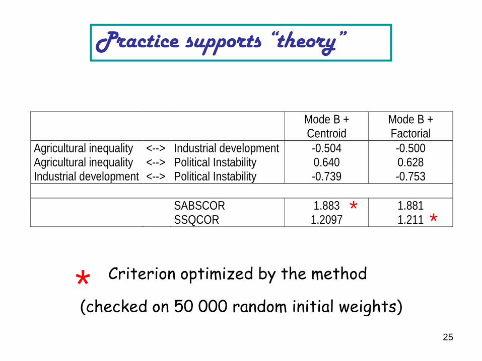
Practice supports “theory”

Mode B + Centroid

Mode B + Factorial

Agricultural inequality <--> Industrial development -0.504 -0.500 Agricultural inequality <--> Political Instability 0.640 0.628 Industrial development <--> Political Instability -0.739 -0.753

SABSCOR 1.883 1.881 SSQCOR 1.2097 1.211

* *

* Criterion optimized by the method

(checked on 50 000 random initial weights)

26

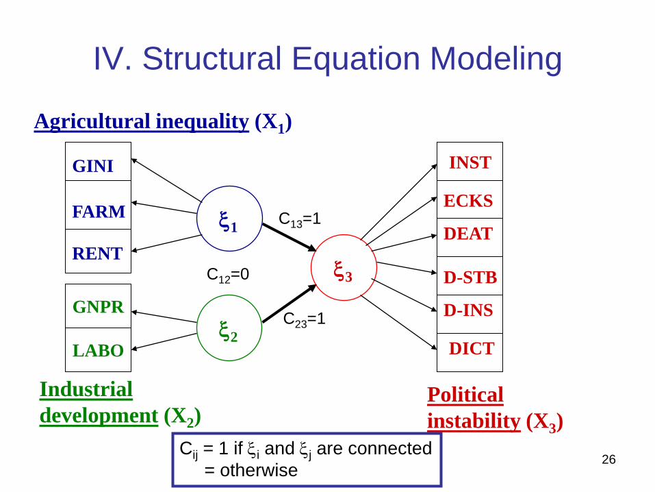
IV. Structural Equation Modeling

GINI

FARM

RENT

GNPR

LABO

Agricultural inequality (X1)

Industrialdevelopment (X2)

ECKS

DEAT

D-STB

D-INS

INST

DICT

Politicalinstability (X3)

ξ1

ξ2

ξ3

C13=1

C23=1

C12=0

Cij = 1 if ξi and ξj are connected= otherwise

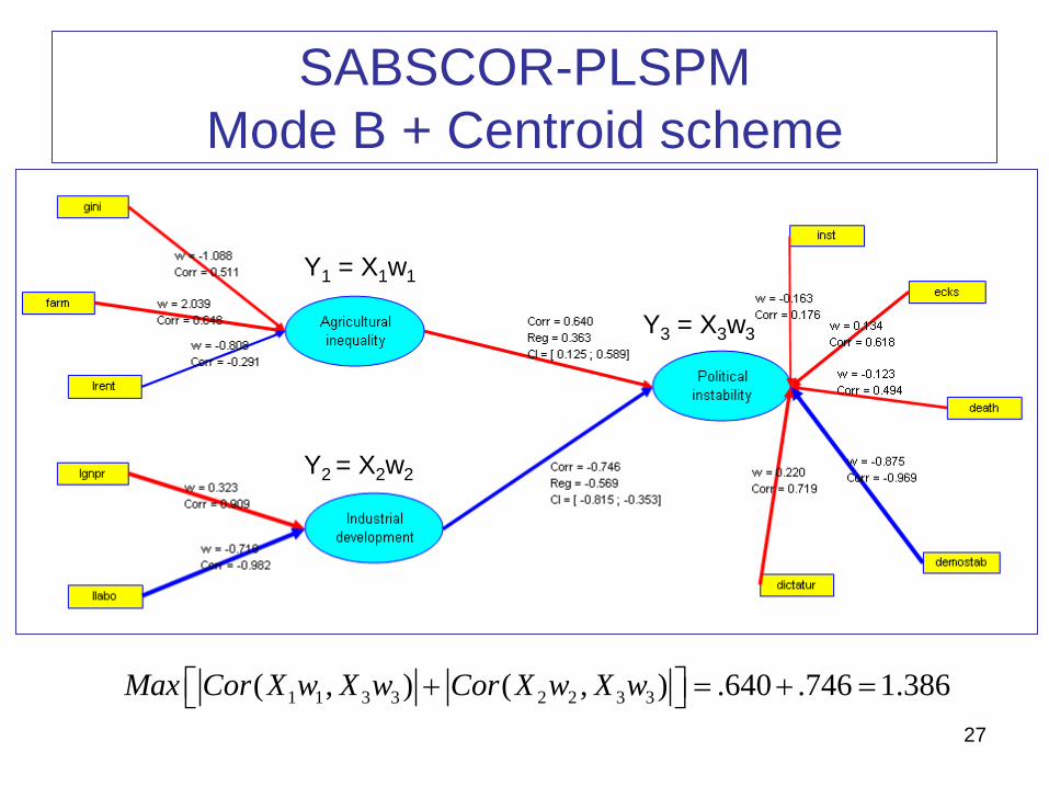
27

SABSCOR-PLSPMMode B + Centroid scheme

Y1 = X1w1

Y2 = X2w2

Y3 = X3w3

1 1 3 3 2 2 3 3( , ) ( , ) .640 .746 1.386Max Cor X w X w Cor X w X w + = + =

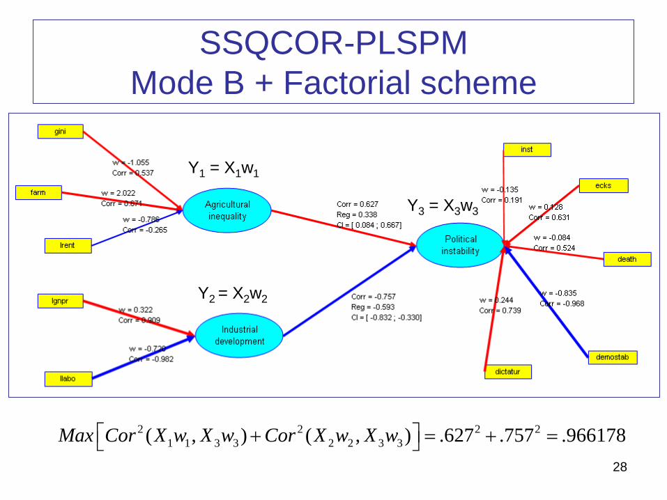
28

SSQCOR-PLSPMMode B + Factorial scheme

Y1 = X1w1

Y2 = X2w2

Y3 = X3w3

2 2 2 21 1 3 3 2 2 3 3( , ) ( , ) .627 .757 .966178Max Cor X w X w Cor X w X w + = + =

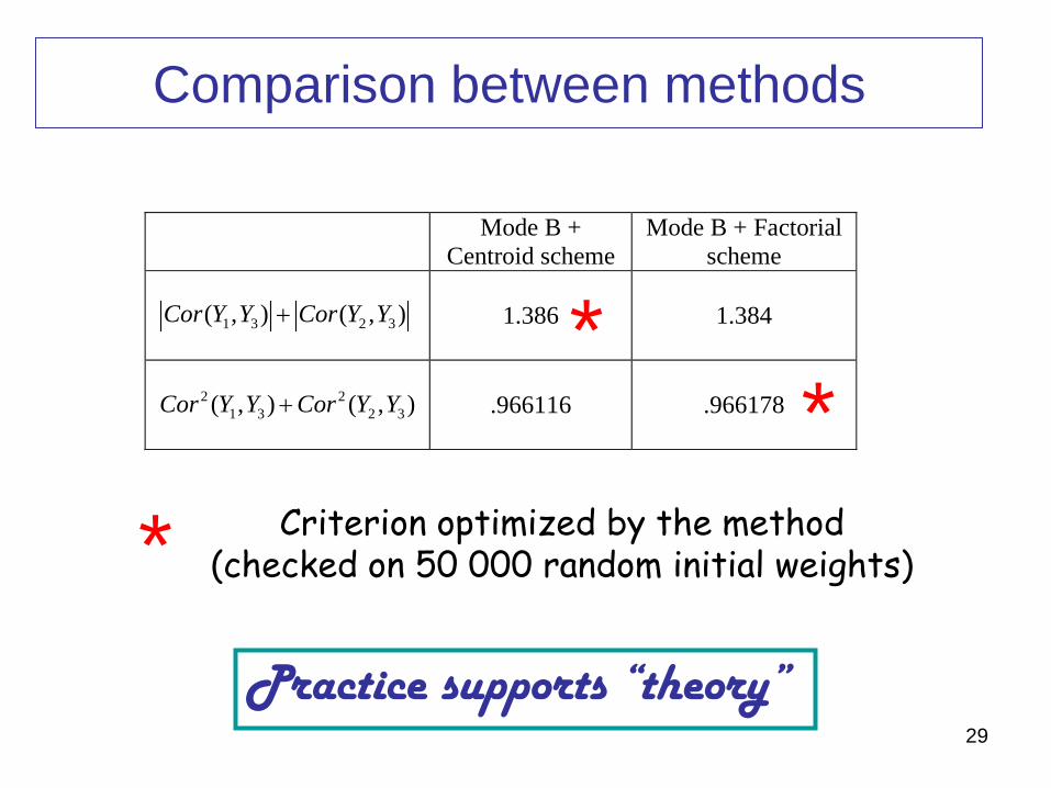
29

Comparison between methods

Mode B + Centroid scheme

Mode B + Factorial scheme

1 3 2 3( , ) ( , )Cor Y Y Cor Y Y+ 1.386 1.384

2 21 3 2 3( , ) ( , )Cor Y Y Cor Y Y+ .966116 .966178

**

* Criterion optimized by the method(checked on 50 000 random initial weights)

Practice supports “theory”

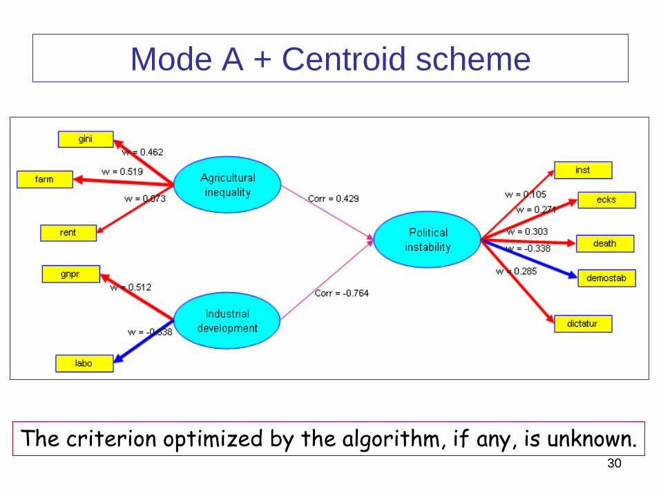
30

Mode A + Centroid scheme

The criterion optimized by the algorithm, if any, is unknown.

31

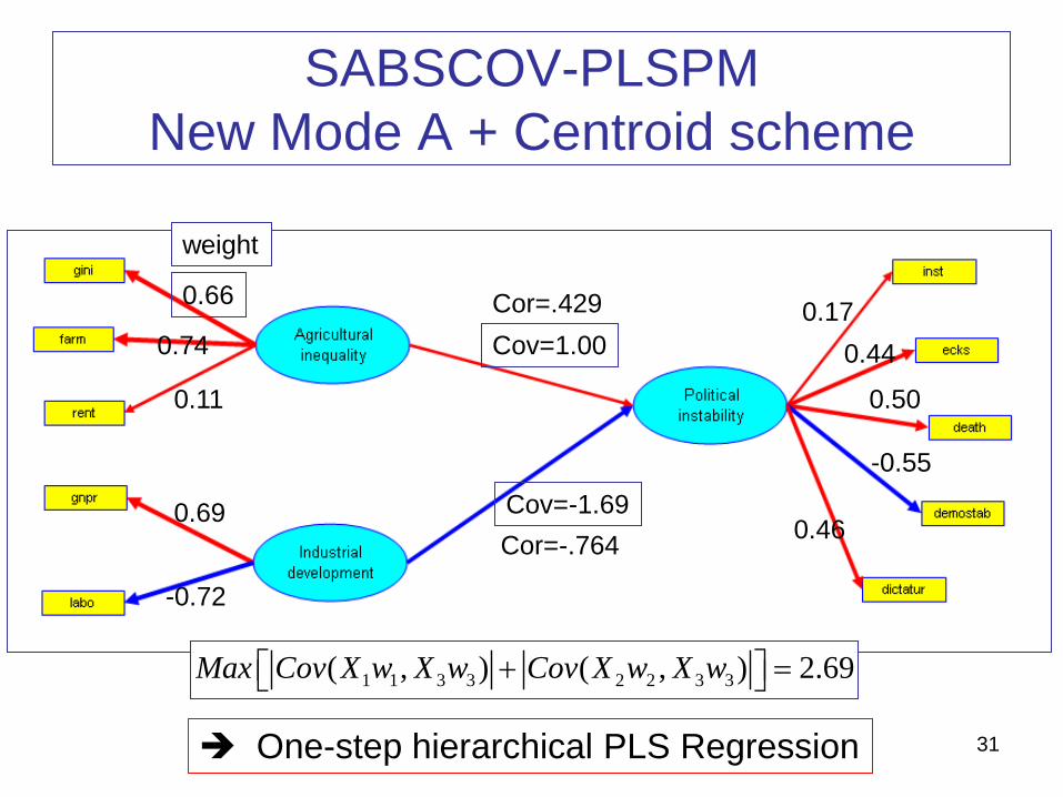
SABSCOV-PLSPMNew Mode A + Centroid scheme

1 1 3 3 2 2 3 3( , ) ( , ) 2.69Max Cov X w X w Cov X w X w + =

0.66

0.74

0.11

0.69

-0.72

0.170.44Cov=1.00

0.50

-0.55

0.46Cov=-1.69

weight

One-step hierarchical PLS Regression

Cor=.429

Cor=-.764

32

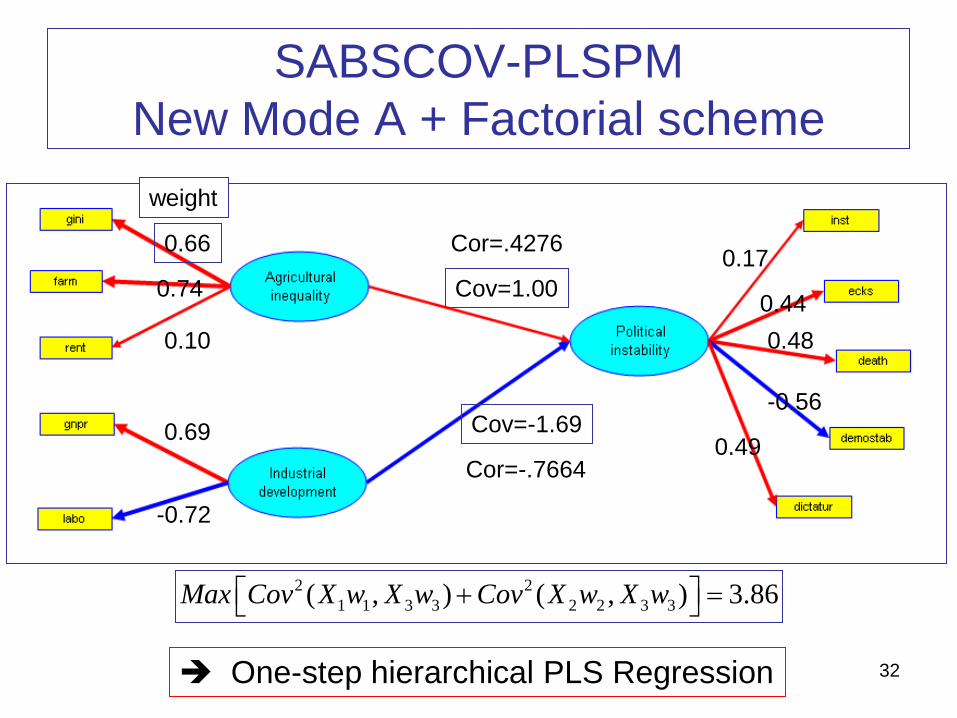
SABSCOV-PLSPMNew Mode A + Factorial scheme

0.66

0.74

0.10

0.69

-0.72

0.17

0.44Cov=1.00

0.48

-0.56

0.49Cov=-1.69

2 21 1 3 3 2 2 3 3( , ) ( , ) 3.86Max Cov X w X w Cov X w X w + =

weight

One-step hierarchical PLS Regression

Cor=.4276

Cor=-.7664

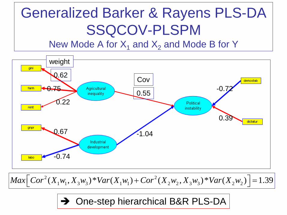
Generalized Barker & Rayens PLS-DASSQCOV-PLSPM

New Mode A for X1 and X2 and Mode B for Y

2 21 1 3 3 1 1 2 2 3 3 2 2( , )* ( ) ( , )* ( ) 1.39Max Cor X w X w Var X w Cor X w X w Var X w + =

0.62

0.75

0.22

0.67

-0.74

0.55

-1.04

-0.72

0.39

weight

Cov

One-step hierarchical B&R PLS-DA

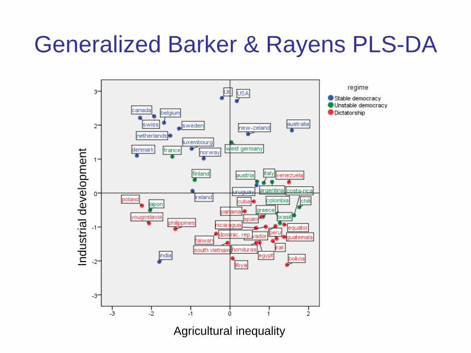
Generalized Barker & Rayens PLS-DA

Agricultural inequality

Indu

stria

l dev

elop

men

t

35

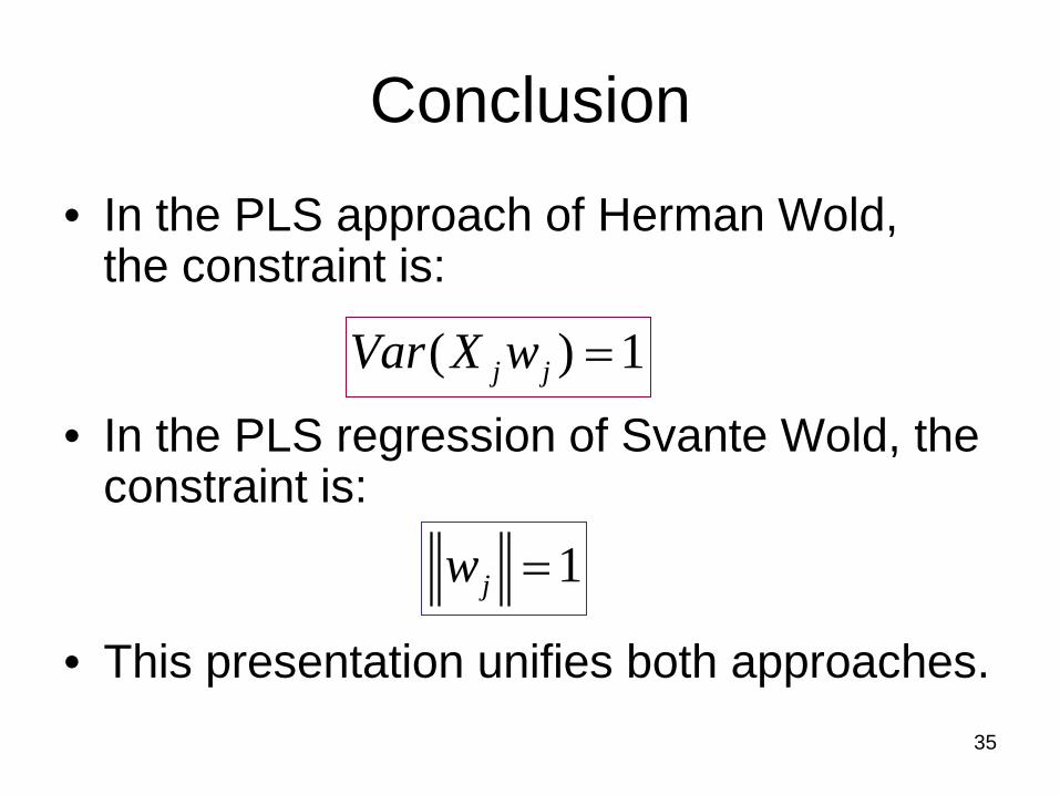
Conclusion

• In the PLS approach of Herman Wold, the constraint is:

• In the PLS regression of Svante Wold, the constraint is:

• This presentation unifies both approaches.

( ) 1j jVar X w =

1jw =