Embed Size (px)
Citation preview
OBJECT-FLOW ANALYSIS FOR OPTIMIZINGFINITE-STATE MODELS OF JAVA SOFTWARE
by
VENKATESH PRASAD RANGANATH
B.E., Bangalore University, 1997
A THESIS
submitted in partial fulfillment of the
requirements for the degree
MASTER OF SCIENCE
Department of Computing and Information ScienceCollege of Engineering
KANSAS STATE UNIVERSITYManhattan, Kansas
2002
Approved by:
Major ProfessorJohn Hatcliff
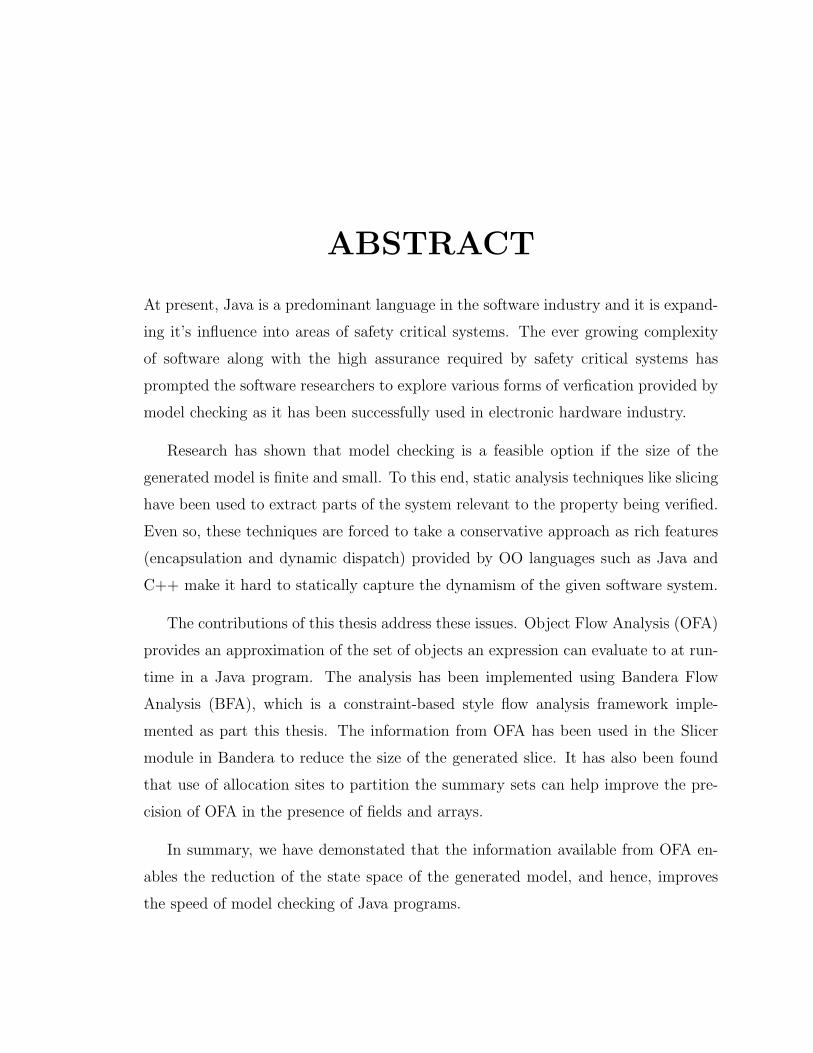
ABSTRACT
At present, Java is a predominant language in the software industry and it is expand-
ing it’s influence into areas of safety critical systems. The ever growing complexity
of software along with the high assurance required by safety critical systems has
prompted the software researchers to explore various forms of verfication provided by
model checking as it has been successfully used in electronic hardware industry.
Research has shown that model checking is a feasible option if the size of the
generated model is finite and small. To this end, static analysis techniques like slicing
have been used to extract parts of the system relevant to the property being verified.
Even so, these techniques are forced to take a conservative approach as rich features
(encapsulation and dynamic dispatch) provided by OO languages such as Java and
C++ make it hard to statically capture the dynamism of the given software system.
The contributions of this thesis address these issues. Object Flow Analysis (OFA)
provides an approximation of the set of objects an expression can evaluate to at run-
time in a Java program. The analysis has been implemented using Bandera Flow
Analysis (BFA), which is a constraint-based style flow analysis framework imple-
mented as part this thesis. The information from OFA has been used in the Slicer
module in Bandera to reduce the size of the generated slice. It has also been found
that use of allocation sites to partition the summary sets can help improve the pre-
cision of OFA in the presence of fields and arrays.
In summary, we have demonstated that the information available from OFA en-
ables the reduction of the state space of the generated model, and hence, improves
the speed of model checking of Java programs.
TABLE OF CONTENTS
List of Figures iv
List of Tables vi
List of Examples viii
Acknowledgments ix
1 Introduction 1
1.1 Model Checking . . . . . . . . . . . . . . . . . . . . . . . . . . . . . . 2
1.2 Static Analysis . . . . . . . . . . . . . . . . . . . . . . . . . . . . . . 6
1.3 Object-oriented Languages . . . . . . . . . . . . . . . . . . . . . . . . 7
1.4 Object-Flow Analysis . . . . . . . . . . . . . . . . . . . . . . . . . . . 10
1.5 Thesis Outline . . . . . . . . . . . . . . . . . . . . . . . . . . . . . . . 11
1.6 Audience . . . . . . . . . . . . . . . . . . . . . . . . . . . . . . . . . . 12
2 Background 14
2.1 Data-Flow Analysis . . . . . . . . . . . . . . . . . . . . . . . . . . . . 14
2.1.1 Program Points . . . . . . . . . . . . . . . . . . . . . . . . . . 15
2.1.2 Locality . . . . . . . . . . . . . . . . . . . . . . . . . . . . . . 15
2.1.3 Context . . . . . . . . . . . . . . . . . . . . . . . . . . . . . . 16
2.1.4 Execution Model . . . . . . . . . . . . . . . . . . . . . . . . . 17
i
2.2 Points-to Analysis . . . . . . . . . . . . . . . . . . . . . . . . . . . . . 20
2.2.1 Andersen’s Algorithm . . . . . . . . . . . . . . . . . . . . . . 23
2.2.2 Steensgaard’s Algorithm . . . . . . . . . . . . . . . . . . . . . 24
2.2.3 Das’ Algorithm . . . . . . . . . . . . . . . . . . . . . . . . . . 26
2.2.4 Liang’s Algorithm . . . . . . . . . . . . . . . . . . . . . . . . . 27
2.3 Inter-Procedural Analysis . . . . . . . . . . . . . . . . . . . . . . . . 29
2.4 Context-sensitivity . . . . . . . . . . . . . . . . . . . . . . . . . . . . 35
2.5 Java . . . . . . . . . . . . . . . . . . . . . . . . . . . . . . . . . . . . 38
2.5.1 Data-Flow Analysis . . . . . . . . . . . . . . . . . . . . . . . . 39
2.5.2 Control-Flow Analysis . . . . . . . . . . . . . . . . . . . . . . 42
3 Object-Flow Analysis 44
3.1 Overview . . . . . . . . . . . . . . . . . . . . . . . . . . . . . . . . . . 44
3.2 Concept . . . . . . . . . . . . . . . . . . . . . . . . . . . . . . . . . . 48
3.2.1 Data-Flow Analysis . . . . . . . . . . . . . . . . . . . . . . . . 49
3.2.2 Object-Flow Analysis . . . . . . . . . . . . . . . . . . . . . . . 51
3.2.3 Details . . . . . . . . . . . . . . . . . . . . . . . . . . . . . . . 52
3.3 In Theory . . . . . . . . . . . . . . . . . . . . . . . . . . . . . . . . . 64
3.3.1 Common Approaches . . . . . . . . . . . . . . . . . . . . . . . 64
3.3.2 Varying Precision in Constraint-based Analysis . . . . . . . . 66
3.4 Constraints for Object-Flow Analysis . . . . . . . . . . . . . . . . . . 74
3.4.1 Flow-insensitive Mode . . . . . . . . . . . . . . . . . . . . . . 74
3.4.2 Flow-sensitive Mode . . . . . . . . . . . . . . . . . . . . . . . 78
3.4.3 Context-sensitive Mode . . . . . . . . . . . . . . . . . . . . . . 81
3.5 Algorithm . . . . . . . . . . . . . . . . . . . . . . . . . . . . . . . . . 83
3.5.1 Complexity . . . . . . . . . . . . . . . . . . . . . . . . . . . . 87
3.6 Fields and Arrays . . . . . . . . . . . . . . . . . . . . . . . . . . . . . 89
ii
3.6.1 Static Fields . . . . . . . . . . . . . . . . . . . . . . . . . . . . 89
3.6.2 Instance Fields . . . . . . . . . . . . . . . . . . . . . . . . . . 90
3.6.3 Arrays . . . . . . . . . . . . . . . . . . . . . . . . . . . . . . . 92
3.6.4 Observations . . . . . . . . . . . . . . . . . . . . . . . . . . . 94
4 The Implementation 95
4.1 Bandera . . . . . . . . . . . . . . . . . . . . . . . . . . . . . . . . . . 95
4.2 Soot . . . . . . . . . . . . . . . . . . . . . . . . . . . . . . . . . . . . 98
4.2.1 Jimple . . . . . . . . . . . . . . . . . . . . . . . . . . . . . . . 99
4.3 BFA: The Underlying Framework . . . . . . . . . . . . . . . . . . . . 101
4.3.1 Variants . . . . . . . . . . . . . . . . . . . . . . . . . . . . . . 101
4.3.2 Managers . . . . . . . . . . . . . . . . . . . . . . . . . . . . . 102
4.3.3 Indices . . . . . . . . . . . . . . . . . . . . . . . . . . . . . . . 102
4.3.4 The Framework . . . . . . . . . . . . . . . . . . . . . . . . . . 105
4.4 OFA: An Instance of BFA . . . . . . . . . . . . . . . . . . . . . . . . 106
5 Application 110
5.1 Program Slicing . . . . . . . . . . . . . . . . . . . . . . . . . . . . . . 110
5.2 Method Inlining . . . . . . . . . . . . . . . . . . . . . . . . . . . . . . 113
5.3 Trivial Optimizations . . . . . . . . . . . . . . . . . . . . . . . . . . . 114
6 Future Work 116
6.1 Current Limitations . . . . . . . . . . . . . . . . . . . . . . . . . . . . 116
6.2 Possible Extensions . . . . . . . . . . . . . . . . . . . . . . . . . . . . 119
Bibliography 124
iii
LIST OF FIGURES
1.1 UML diagram for the producer class hierarchy problem. . . . . . . . . 9
2.1 An illustration of how variables are related to each other in a simpleinteger swapping program in C. . . . . . . . . . . . . . . . . . . . . . 18
2.2 An illustration of how variables are related in a pointer value swappingprogram in C. . . . . . . . . . . . . . . . . . . . . . . . . . . . . . . . 21
2.3 An illustration of variables and their points-to set generated by usingAndersen’s algorithm to analyze an pointer value swapping C programin example 2.2 without line 16. . . . . . . . . . . . . . . . . . . . . . 23
2.4 An illustration of variables and their points-to set generated by us-ing Steensgaard’s algorithm to analyze the pointer value swapping Cprogram in example 2.2 without line 16. . . . . . . . . . . . . . . . . 25
2.5 An illustration of Liang’s algorithm in various phases when applied tothe pointer value swapping C program given in example 2.2. . . . . . 28
2.6 The call graph for the source code given in example 2.2. . . . . . . . 30
2.7 Illustration of the circularity between inter-procedural analysis and callgraph construction. . . . . . . . . . . . . . . . . . . . . . . . . . . . . 33
2.8 Snapshots of the call graph as call graph construction and inter-proceduralanalysis proceed in tandem. . . . . . . . . . . . . . . . . . . . . . . . 34
3.1 Representation of the flow equations for line 39 in example 3.1 as agraph. . . . . . . . . . . . . . . . . . . . . . . . . . . . . . . . . . . . 55
3.2 Partial Value flow graph for the program given in example 3.1. . . . . 60
3.3 Flow graph capturing flow-insensitive information for the program inexample 3.1. . . . . . . . . . . . . . . . . . . . . . . . . . . . . . . . . 62
iv
3.4 State of heap during the creation and assignment to arrays. . . . . . . 93
4.1 The architecture of Bandera tool set. . . . . . . . . . . . . . . . . . . 97
4.2 The class diagram of variants. . . . . . . . . . . . . . . . . . . . . . . 103
4.3 The class diagram of managers. . . . . . . . . . . . . . . . . . . . . . 104
4.4 The class diagram of BFA framework. . . . . . . . . . . . . . . . . . . 107
4.5 The class diagram of Object-flow analysis. . . . . . . . . . . . . . . . 109
v
LIST OF TABLES
2.1 Result of performing a flow-insensitive, context-insensitive and inter-procedural DFA on a simple integer swapping program in C. . . . . . 19
2.2 Result of performing a flow-insensitive, context-insensitive, and inter-procedural,PTA on a pointer value swapping program in C. . . . . . . 22
3.1 Result of Flow-insensitive, context-insensitive, inter-procedural object-flow information for the Family code. . . . . . . . . . . . . . . . . . . 46
3.2 Data flow equations templates for the expressions, int and new, andfor assignment statement in Java. . . . . . . . . . . . . . . . . . . . . 54
3.3 Flow equations for a few selected statements that contribute to valueflow in the program in example 3.1 . . . . . . . . . . . . . . . . . . . 57
3.4 Summary of value flow in the program given in example 3.1. . . . . . 63
3.5 C after performing object flow analysis on Test class in the variousmodes described earlier. . . . . . . . . . . . . . . . . . . . . . . . . . 70
3.6 ρ after performing object flow analysis on Test class in the variousmodes described earlier. . . . . . . . . . . . . . . . . . . . . . . . . . 71
3.7 Object-Flow analysis constraint templates corresponding to expression-statements in Java. . . . . . . . . . . . . . . . . . . . . . . . . . . . . 77
3.8 Object-Flow analysis constraint templates corresponding to pure atomicexpressions in Java. . . . . . . . . . . . . . . . . . . . . . . . . . . . . 78
3.9 Flow-insensitive mode constraints for the methods foo and bar definedin example 3.3. . . . . . . . . . . . . . . . . . . . . . . . . . . . . . . 79
3.10 Flow-sensitive mode constraints for foo method defined in example 3.3. 81
vi

3.11 Flow and Context-sensitive mode constraints for bar method definedin example 3.3. . . . . . . . . . . . . . . . . . . . . . . . . . . . . . . 83
vii
LIST OF EXAMPLES
1.1 Dynamic dispatch in action. . . . . . . . . . . . . . . . . . . . . . . . . . 8
2.1 DFA in the presence of pure value-based variables. . . . . . . . . . . . . 18
2.2 DFA in the presence of pointer variables. . . . . . . . . . . . . . . . . . . 21
2.3 The concept of first-class functions in other languages. . . . . . . . . . . 31
2.4 Call graph construction and inter-procedural analysis. . . . . . . . . . . . 33
2.5 Calling sequences, object oriented languages, and contexts. . . . . . . . . 36
3.1 Object Flow Analysis . . . . . . . . . . . . . . . . . . . . . . . . . . . . . 44
3.2 Value Flow Analysis . . . . . . . . . . . . . . . . . . . . . . . . . . . . . 55
3.3 Object Flow Analysis in various modes of operation. . . . . . . . . . . . 68
5.1 Program slicing and Object-flow analysis information. . . . . . . . . . . . 111
5.2 Method inlining and Object-flow analysis information. . . . . . . . . . . 113
viii

ACKNOWLEDGMENTS
To be involved in a research project is a great experience.
I am thankful to Dr.Matthew Dwyer for offering me an opportunity (which I
did grab!) to work in BANDERA group. I am thankful to Dr.John Hatcliff, my
major professor, for being patient and persistent while guiding and mentoring me
while working on this thesis. I am thankful for the numerous opportunities they both
gave me to be involved in activities other than my thesis, and most of all for being
enthusiastic and supportive. I am also thankful to Dr.Anindya Banerjee for providing
useful inputs during the preparation of the thesis.
I am thankful to the entire BANDERA group for providing a great working envi-
ronment. In particular, I am thankful to Hongjun Zheng for being a rigorous tester
of my implementation. I am thankful to my friends for bearing with my antics, and
making the long hot summers and bitter cold winters bearable.
I am thankful to my wife, Prathima, for being patient and supportive during my
indulgence with my workstation for long hours and for bearing with my rather erratic
feeding habit.
They say, save the best for last. Hence, lastly I would like to thank my mother,
my father, and my elder sister for advising me in the ways of life and helping hold
the helm during storms. “Home is the first school” is an adage in Kannada. I am
indebted to my family for providing a great first school.
ix
Chapter 1
Introduction
Software has become a banality from a rarity in the last two decades. Today, software
can be found in a whole array of gadgets and devices, from a simple day-to-day gadget
like a wrist watch to something as complex and critical as a Boeing-747. Various
facilities for deploying software and hardware are becoming an integral part of the
infrastructures being built in the wake of the new millennium. Such is the impact of
software on the society in the present day.
Historically, whenever a new technology was adapted in everyday life, safety was
given the highest priority. Likewise the software, which controls the present day-
to-day devices, in particular the software that controls complex and safety critical
devices has come under scrutiny. How safe is the software that assists a human
pilot to control a Boeing-747? Or how safe is the software that monitors radiology
treatment? If software has to be accepted for everyday use, there should be some
sound way to declare software as safe.
The word, “safe”, needs to be well defined before speaking about safety. A rea-
sonable definition of safe would be, “It is a condition in which there is no harm of
any sort to life and property”. Now safety in the context of software means that, at
all times, the software should not void the condition of being safe. Also, the software
should try to maintain the condition of being safe. The first part of the meaning is
1
CHAPTER 1. INTRODUCTION
of primary interest to us.
The current practice in today’s software “factories” to ensure quality, and hence
safety, is through testing. Testing can be used to ensure if the software satisfies the
requirements and also does not fail critically. In this regard, testing is useful and
will be indispensable in the software industry. This said, due to rapid technological
advances, the systems being built today are far more complex when compared to those
built a few years ago. With an ever-expanding market, which is trying to outrun itself,
the time span from the conception of an idea to it’s realization as a product in the
market is diminishing. Both these factors put together, it becomes highly unlikely to
create a product that satisfies the given requirements and specification in the given
time frame. When the product has added safety concerns, it only aggravates the task
on hand.
1.1 Model Checking
One promising technology to establish software safety is Model Checking.
Model Checking1 is the technique wherein an abstract model of the system is con-
structed and then the model is “automatically” checked to satisfy various properties
that the actual system should satisfy. The key here is that the check needs to be done
automatically. This is because machines are better in executing repetitive tasks than
humans and speaking cost-wise, it is expensive to expend human effort for repetitive
programmable tasks.
This technique has been successfully used in the hardware industry through model
checkers like SMV[McM93] to verify VLSI chip design and in software industry
through model checkers like Spin[Hol97] to verify network protocols.
As the cost per unit of computing power is decreasing and the safety concerns
in systems monitored by software is increasing, the software community at large has
1Please refer to [MOSS99] for a good introduction to Model Checking.
2
CHAPTER 1. INTRODUCTION
begun to explore the possibility of using model checking to verify software. It all
started by the application of model checking to verify network protocols. Given the
complexity of the present-day software, the problem of verifying in a reasonable time
frame if software satisfies a large set of properties is intractable. Hence, a possible
way out would be to construct a model of the system and perform the check on it.
In simple words, model checking software is a brute-force method of verifying if
software or a system2 satisfies a set of properties at all times during it’s execution. As
mentioned earlier, it involves constructing a model of the system, computing all the
possible states of the model, and then checking if the given properties are satisfied in
all of these states. The State of the model represents the collection of various variables
and their values in the software at a certain point along a certain path of execution.
The constructed model should possess the following properties for model checking
to be a feasible and tractable solution, and also for the results to be correct.
Accuracy The capacity to draw valid conclusions about the software by verifying a
property on a model of the software depends on accuracy with which the various
characteristics of the software are captured in the model. These characteristics
may be static characteristics like all the possible values associated with a vari-
able or dynamic characteristics like the possible branch after the computation
of the conditional expression.
It may be possible to verify a property of the software without capturing all the
characteristics of the software in the model.
A classic example would be the signs example. If an unsigned integer variable
is modeled as 32 bit value then the size of the value domain of the variable is
232. If it is know a priori that only the polarity of the value of the variable bears
relevance to the property being checked, then the variable can be modeled as a
new type which can take on values: pos, zero, and neg, where each of these value
represents the polarity of the value bound to the variable. This technique is
2From hereon, software and system shall be used interchangeably unless mentioned otherwise.
3
CHAPTER 1. INTRODUCTION
known as data abstraction . It should be noted that the property being checked
dictates the required level of accuracy while modeling the software.
In a situation like the above example the definition of accuracy in terms of
characteristics of the software is too strong. So a weaker but sound definition
would be that the model should be able to simulate3 all possible paths in the
software. More precisely, for every valid execution path in the software there
should be a corresponding path in the model. In such a situation, if a property
holds along one such path in the model, it will also hold along the corresponding
path in the software.
Since the definition of simulation is not bi-directional, it is possible to have
paths in the model with no corresponding paths in the software. These paths
are termed as infeasible paths. This is true in most cases as a result of the
combination of data abstraction and conditionals. The result of a property
either failing or holding along one such path in the model does not bear relevance
to the software. The situation where model checking fails to verify a property
because of violation of the property along an infeasible path is called false
negative.
State-Space of the Model The total number of states in a model is called the
state-space of the model or size of the model. As the properties are to be verified
at states of the model, the state-space of the model should be finite (and small)
for automatic model checking to be feasible and tractable. Such models are
called finite-state models 4.
One way of achieving a finite state-space is through constructing abstract models
of the software in which the property being checked dictates the possible level of
abstraction at which various characteristic of the software can be modeled. If
certain characteristics of the software, such as the set of values a variable can
take on, are not abstracted, then the state-space of the model may be too large
3For further discussion on simulation, refer to [Dam96].4From now on finite-state models and models shall be used interchangeably unless mentioned
otherwise.
4
CHAPTER 1. INTRODUCTION
for model checking to be a feasible and tractable solution. This motivates the
abstraction mentioned earlier in the signs example.
The size of the state-space of a model increases by a factor proportional to
the size of value domains of variables occurring in that model. Although most
model checkers employ various state-space reduction techniques, still the time
taken to check a property of a model with inherently smaller state-space is less
compared to that of a model with a larger state-space. In the signs example, if
the unsigned integer variable is represented as is in the model, then the size of
the state-space of the model will increase by a factor of 232. On the other hand,
if it is abstracted judiciously as described previously, the size of the state-space
increases by a factor of 3, which is a drastic difference. Here again a combination
of abstraction and conditionals may bloat up the state-space but it can still be
curbed to stay closer to the lower limit.
It is clear from the above properties that there are two mutually opposing proper-
ties involved when constructing such a model, accuracy and state-space (size) of the
model. Although it is not valid to claim that it is impossible to construct a model that
is highly accurate and has a minuscule state-space, in almost all cases the accuracy
and the size of the state-space are inversely proportional. Hence, one of the current
lines of research is to find new ways to control state-space explosion, i.e., to reduce the
size of the state-space of the model. This includes finding new abstraction techniques
driven by relevant property to abstract various characteristics of the software such
that drastic state-space reductions occur but the accuracy required for checking the
property is preserved.
If software needs to be subjected to model checking, then there needs to be an ar-
tifact pertaining to the software that can be subjected to model checking. At present,
as software engineering is young compared to other engineering disciplines, there are
no well defined, widely accepted and standardized artifacts that are generated during
software development cycle apart from the source code pertaining to the software.
Hence, model checking the source code of software is a good approach to model check
5
CHAPTER 1. INTRODUCTION
a software, but not the only one. This approach has the following advantages:
- Programming languages are formal enough to extract properties.
- Programming languages are, by far, the most commonly agreed upon standards
in the software industry.
- Existing systems, as well as, systems being newly designed can benefit from the
same technique.
On the downside, it is not a trivial task to find reasonable abstractions to all entities
in the system.
Bandera[CDH+00] is a tool set aimed at verifying Java software using model check-
ing. This is the product of an on-going project with the same name at Kansas State
University, USA. At a high level, the tool set is capable of extracting a model from a
given Java program, representing the model in the input language of the chosen model
checker, running the model checker over the model and the specified properties, map-
ping the results of model checking back into the Java program, and presenting it in
a user-friendly form. It uses techniques like abstraction-based program specialization
and program slicing to prune the state-space of the extracted model.
1.2 Static Analysis
The model and the properties have to be represented in a formal language understood
by a model checker. Hence, the process of constructing a model of a system can be
viewed as compiling an automatically check-able model from the source code of the
given system.
Compiler technology uses various static analyses to optimize the object code. A
good example would be constant propagation and constant folding. In constant propa-
gation, a variable in an expression will be replaced by a constant if it is known that
6
CHAPTER 1. INTRODUCTION
the value of the variable will always be that constant. After few such replacements,
some expressions will be partially evaluated if they contain sub-expressions with no
variables. This latter optimization is termed as constant folding. This improves run-
time performance at the cost of increased compile-time. If such static analyses can be
suitably adapted for the compilation of the model then they can be used to generate
optimized models of the software and control state-space explosion.
1.3 Object-oriented Languages
The popularity of object-oriented languages is due to the support available for con-
cepts like inheritance and dynamic dispatch.
Inheritance or Subtyping5 provides the capability to inherit properties from an-
other software entity. In terms of object-oriented languages, a software entity, i.e., an
object, can inherit interface or implementation or both from another software entity.
Usually inheritance is used to specialize. This means that the inheriting class or
subclass (subtype) is more specific than the inherited class or superclass (supertype)
in terms of implementation. Hence, the specialization of a class calls for methods
affected by the specialization to be reimplemented by the subclass and the rest of the
methods to be inherited from the superclass. This concept of defining methods in the
subclass that were declared or defined earlier in the superclass is known as method
overriding.
Usually, inheritance is additive. This means that the subclass may have new
properties, but all the inherited properties will be retained. This implies that the
object of the subclass can be used in place of an object of the superclass, as the
subclass has all the properties of the super class and more, but not less.
Hence, a reference variable declared to refer to a type, say X, can refer to an object,
5The concept of inheritance discussed here is strongly tied to those supported in languages likeC++ and Java.
7
CHAPTER 1. INTRODUCTION
which is an instance of a subclass of X. In case a method is invoked (dispatched) on
such a variable and if both the super-type and the subtype implement the invoked
method, which implementation should be executed? The reason for such a situation
is that there are two viable implementations that can be executed, one as a result of
the static type of the variable and the other as a result of the actual type of the object
at the method invocation site (call-site) at run-time. Usually it is resolved in favor
of the implementation provided by the type of the object arriving at the call-site at
run-time. This concept of invoking the method provided by the type of the object
(dynamic type of the variable) arriving at the call-site at run-time is referred to as
dynamic dispatch.
At run-time, dynamic dispatch occurs by checking if the class of the object im-
plements the method to be dispatched. For this check to be possible each class has
an associated Vtable (virtual table) that maps a method signature to a method im-
plementation. If the class does not implement the method then its Vtable contains
an entry indicating that the Vtable of the superclass needs to be referred to for the
implementation. This process of following the chain of links to arrive at a viable im-
plementation is termed as virtual method lookup. Due to this fact, dynamic dispatch
is also called as virtual method invocation.1.1
Example 1.1 (Dynamic dispatch in action.)
Consider a variant of the classic producer-consumer problem. Let there be classes
Producern (Consumern ) representing Producers (Consumers) who can produce
(consume) 1, 2, or 3 units at a time.
In each of the subclasses of Producer, the produce method is redefined. Similarly,
the consume method is redefined in each of the subclasses of Consumer class.
At line 4 the type of p and the type of the object to which it refers are different,
i.e., the type of p is Producer and it refers to an instance of Producer3 class. A
similar situation occurs at line 11 with the distinction that the possible type of objects
to which p refers to are Consumer3 and Consumer1. As explained earlier this leads
8
CHAPTER 1. INTRODUCTION
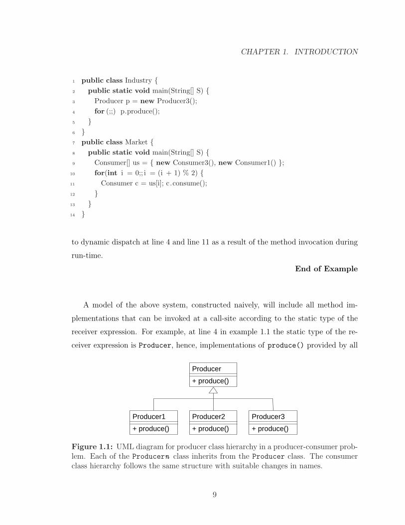
1 public class Industry {2 public static void main(String[] S) {3 Producer p = new Producer3();4 for (;;) p.produce();5 }6 }7 public class Market {8 public static void main(String[] S) {9 Consumer[] us = { new Consumer3(), new Consumer1() };
10 for(int i = 0;; i = (i + 1) % 2) {11 Consumer c = us[i]; c.consume();12 }13 }14 }
to dynamic dispatch at line 4 and line 11 as a result of the method invocation during
run-time.
End of Example
A model of the above system, constructed naively, will include all method im-
plementations that can be invoked at a call-site according to the static type of the
receiver expression. For example, at line 4 in example 1.1 the static type of the re-
ceiver expression is Producer, hence, implementations of produce() provided by all
Producer2
+ produce()
Producer3
+ produce()
Producer
+ produce()
Producer1
+ produce()
Figure 1.1: UML diagram for producer class hierarchy in a producer-consumer prob-lem. Each of the Producern class inherits from the Producer class. The consumerclass hierarchy follows the same structure with suitable changes in names.
9
CHAPTER 1. INTRODUCTION
the subclasses of Producer should be considered at the call-site in the model. This
happens as there is no information that can guarantee the exact implementations that
will be invoked at the call-site. Such a model is called pessimistic or conservative or
over-approximated as it encompasses parts of the system which are highly unlikely to
be executed in reality.
In general, an approach is said to be pessimistic when it handles the most general
scenario. It is also called as conservative as it makes no assumptions about the
specificness of the scenario but rather assumes all probable situations are possible
and tries to handle all of them.
In Example 1.1, by analyzing the program it can be known that p will always
evaluate to an instance of Producer3 at line 4. This sort of information can be used
to optimize the program and the corresponding model of the program by avoiding
consultation of VTable. The information can be used to optimize the model by only
considering the implementation of the produce method in Producer3 class at line 4
and hence reducing the size of the model. In fact, depending on the language of the
model checker being used, the method implementation can be in-lined at the call-site.
A similar optimization is possible at line 11. In this case the method implemen-
tation to be considered at the call-site cannot be narrowed to one implementation,
but nevertheless can be narrowed down from three to two possible implementations
which can reduce the size of the resulting model.
1.4 Object-Flow Analysis
Object-Flow Analysis is the process of collecting data about the sites into which the
objects in a program can flow at run-time.
Object-flow analysis can be used to statically determine all possible objects (these
do not include the objects that may flow in through the external environment) that
flow into a dynamic dispatch site at run-time and hence predict the exact types the re-
10
CHAPTER 1. INTRODUCTION
ceiver will evaluate to at run-time. This information can be used to include only those
method definitions into the model which will be executed during run-time and hence,
control state-space explosion. This optimization occurs while considering methods
for program slicing and in-lining during the construction of models from source code
in Bandera tool set. The same analysis can also yield information indicating if a
variable will evaluate to null at a particular site in the program. This information
can be used to improve the process of checking a generated model. All of these ideas
will be discussed in greater detail in subsequent chapters.
This thesis demonstrates that Object-Flow analysis can be used to optimize the
finite-state models of OO systems. As flow graph construction is the core of Object-
Flow analysis, an in-depth examination of the flow-graph construction forms a major
part of this thesis. The main contributions of this thesis are as follows:
• a general algorithm to construct flow graph for systems written in Java pro-
gramming language is presented,
• a Java implementation of the algorithm is provided as part of Bandera tool set,
and
• an illustration of how various program transformations such as slicing and inlin-
ing can use information from the algorithm to help curtail state-space explosion
are explored.
1.5 Thesis Outline
The rest of the thesis is organized as follows:
• Chapter 2 provides a brief introduction to data-flow analysis followed by the
review of three points-to analyses specific to C programming language (in liter-
ature). This is followed by topics close to that presented in chapter 2 of David
Grove’s PhD thesis. Grove’s thesis is relevant for it’s description of how to tackle
11
CHAPTER 1. INTRODUCTION
the circularity between call-graph construction and inter-procedural analysis
and also the description of how to achieve context-sensitive inter-procedural
analysis in the realm of object-oriented languages. The chapter concludes by
presenting how optimization of finite-state models of Java programs can benefit
from these techniques.
• Chapter 3 starts with an example justifying the need for object-flow analysis.
It is followed by an explanation of what is object-flow analysis and how is it
achieved. The explanation proceeds at an abstract level independent of any
intermediate representation. It also reviews how various levels of precision can
be achieved in flow analysis.
• Chapter 4 presents the setting in which the object-flow analysis is implemented.
This is followed by the details about the design and implementation of the
analysis in Java.
• Chapter 5 provides instances of the Slicer and Inliner modules of Bandera tool
set where the information from object-flow analysis is used to optimize the
finite-state model of a system in terms of number of states. An explanation of
how other simple analyses (can) use information from object-flow analysis to
optimize the finite-state model concludes the chapter.
• Chapter 6 concludes the thesis with approaches in which the algorithm and the
implementation can be extended to obtain more precise object-flow information
and configured dynamically to vary the precision of the analysis. It also provides
suggestions on how the path-conscious (flow-sensitive) object-flow analysis can
be used to optimize other program transformations like slicing.
1.6 Audience
The reader is assumed to have the background about programming languages in
terms of how their semantics are discussed in theory, how programming languages
12
CHAPTER 1. INTRODUCTION
are implemented, and how various features of the object language influences it’s im-
plementation. Also, familiarity with the fundamentals of compiler technology to the
extent of how the features of the object language influences compilation is assumed.
It is assumed that the reader is well versed with Java technology. It helps if the reader
has programmed in C as some initial examples are programmed in C.
13
Chapter 2
Background
This chapter provides a brief introduction to data-flow analysis followed by the review
of three points-to analyses specific to C programming language (in literature). This
is followed by topics close to that presented in chapter 2 of David Grove’s PhD thesis.
Grove’s thesis is relevant for it’s description of how to tackle the circularity between
call-graph construction and inter-procedural analysis and also the description of how
to achieve context-sensitive inter-procedural analysis in the realm of object-oriented
languages. This chapter concludes by discussing the previous ideas in the context of
Java.
2.1 Data-Flow Analysis
Data Flow Analysis is a form of static analysis. Static analysis means an analysis
performed without executing the code being analyzed.
Data Flow Analysis (DFA) is a process of statically collecting information per-
taining to the flow of data (values) in a given program at run-time. The collected
information can be used to optimize the code being generated by compilers. A good
example would be constant propagation which was discussed in the previous chapter.
14
CHAPTER 2. BACKGROUND
Since DFA is all about collecting information pertaining to data-flow at run-time,
the DFAs can be classified depending on the sort of information collected. These clas-
sifications are usually orthogonal, i.e., algorithms belonging to different classifications
can be merged. From hereon, the information collected pertaining to a variable will
be referred to as the summary set corresponding to the variable.
2.1.1 Program Points
The first classification is based on the accuracy of the information corresponding to a
program point. A program point in a program may correspond to a line, a statement
or an expression.1 If it is possible to obtain information pertaining to a variable
specific to a program point in the system, then the DFA is flow-sensitive. Otherwise
the DFA is flow-insensitive.
If the DFA is flow-sensitive then each variable is associated with a summary set at
each program point and it is expensive to maintain such information as the number
of such program points may be large in a real world system. On the other hand, if the
DFA is flow-insensitive, there will be one summary set associated with each variable
in the system which is comparatively less expensive.
2.1.2 Locality
The second classification is based on the locality of the data-flow. If the collected
information is local to the body of a procedure, i.e., the information pertains to the
data-flow within a procedure without considering external data, then the DFA is
intra-procedural. If the collected information pertains to the flow of data across the
boundaries of procedures as a result of procedure calls, then DFA is inter-procedural2.
Intra-Procedural DFA analysis requires the summary set to capture only the data-
1This definition differs from the one in [Muc97] on page 303.2For further discussion of inter/intra-procedural analysis, refer to section 2.3.
15
CHAPTER 2. BACKGROUND
flow inside a procedure. This means each procedure can be analyzed independently
of other procedures and also procedure calls do not affect the analysis. Hence, the
analysis is cheap in terms of time and space.
On the other hand, inter-procedural analysis will be affected by procedure calls
existing in the system. In particular, inter-procedural analysis will be affected by
parameter-passing procedure calls or procedures with return values, i.e., function-
like procedures. As data-flow occurring across procedural boundaries resulting from
parameter-passing needs to be captured, the data-flow in the caller procedure and the
callee procedure will be connected suitably. This means that the number of values
flowing and the paths along which they flow will increase. Due to the high cost of
tracking and maintaining such information, the overall cost of inter-procedural DFA
is greater than intra-procedural DFA.
2.1.3 Context
The third classification is based on calling context serving as a means of classifying
collected information. Typically, a calling context can be equivalent to a part or the
whole of call stack during the execution of the program.3 If it is possible to obtain
information specific to a calling context, then the DFA is context-sensitive. Otherwise
the DFA is context-insensitive. In general, any information can serve as a context.
For example, program points are a valid contexts which result in flow-sensitive DFA.
However, the context must be chosen in such a manner that the precision of the
analysis improves and the cost of involving the context in terms of space is as low as
possible.
In a context-insensitive analysis, the nested procedure calls (procedure calls en-
closed in the body of other procedures) do not have any impact on the collection of
information. In case of context-sensitive analysis, for each procedure, more than one
3Please refer to section 2.4 for further discussion on context-sensitivity in object-oriented lan-guages.
16
CHAPTER 2. BACKGROUND
set of information needs to be maintained depending on the procedures in the call
stack. For example, if a procedure A is called by two other procedures B and C, and
the length of the context to be considered is 2, then there will be two sets of data-flow
information for A, one specific to when A was called from B (BA) and other specific
to when A was called from C (CA). If the length of the calling context is 3 and B is
called in M and N, and C is called in N and P, then there will be an information set
for the calling sequences, MBA, NBA, NCA, and PCA. Technically, the number of
information sets for a variable in a context-sensitive analysis will be the number of
distinct sequences of procedures in the call stack with the following properties:
- Each sequence should be possible at run-time.
- Each sequence should end with the procedure enclosing the variable.
- Each sequence can be no longer than the given length.
It is evident that such information can grow rapidly in a large system and hence the
cost to track and maintain such information will be high.
2.1.4 Execution Model
The fourth classification is really a variation or an extension of flow-(in)sensitive DFA
in the presence of multi-threading. If the information collected is thread-sensitive,
i.e., reflects the flow of data according to various thread schedule sequences, then the
DFA is thread-sensitive. Otherwise the DFA is thread-insensitive.
This is a classification that is usually not implemented as it is very expensive. In
general, the number of sequences in which two assignments statements, say X and
Y, can execute in a multi-threaded environment is 2, i.e., XY and YX. Hence, in the
presence of many such statements, the number of sequences increase exponentially
and it is likely that the amount of data-flow information maintained for each variable
will follow closely. In other words, this mode of analysis is the collection of information
17
CHAPTER 2. BACKGROUND
over many static executions of the given system such that all possible execution paths
are exhausted. In that case, using model checking based static analysis may be better.
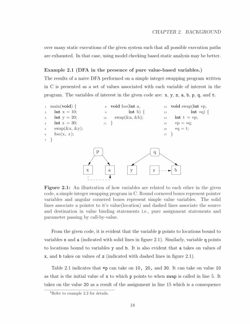
Example 2.1 (DFA in the presence of pure value-based variables.)
The results of a naive DFA performed on a simple integer swapping program written
in C is presented as a set of values associated with each variable of interest in the
program. The variables of interest in the given code are: x, y, z, a, b, p, q, and t.
1 main(void) {2 int x = 10;3 int y = 20;4 int z = 30;5 swap(&x, &y);6 foo(x, z);7 }
8 void foo(int a,9 int b) {
10 swap(&a, &b);11 }
12 void swap(int ∗p,13 int ∗q) {14 int t = ∗p;15 ∗p = ∗q;16 ∗q = t;17 }
x a y z b
qp
Figure 2.1: An illustration of how variables are related to each other in the givencode, a simple integer swapping program in C. Round cornered boxes represent pointervariables and angular cornered boxes represent simple value variables. The solidlines associate a pointer to it’s value(location) and dashed lines associate the sourceand destination in value binding statements i.e., pure assignment statements andparameter passing by call-by-value.
From the given code, it is evident that the variable p points to locations bound to
variables x and a (indicated with solid lines in figure 2.1). Similarly, variable q points
to locations bound to variables y and b. It is also evident that a takes on values of
x, and b takes on values of z (indicated with dashed lines in figure 2.1).
Table 2.1 indicates that *p can take on 10, 20, and 30. It can take on value 10
as that is the initial value of x to which p points to when swap is called in line 5. It
takes on the value 20 as a result of the assignment in line 15 which is a consequence
4Refer to example 2.2 for details.
18
CHAPTER 2. BACKGROUND
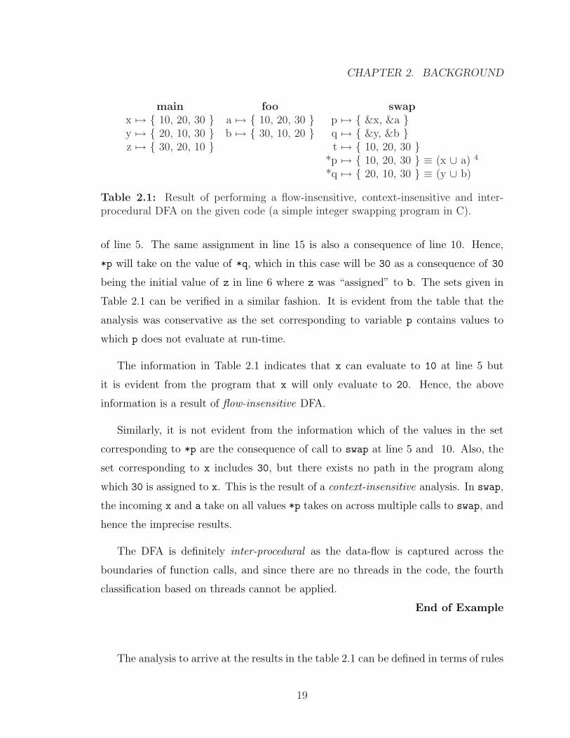
main foo swapx 7→ { 10, 20, 30 } a 7→ { 10, 20, 30 } p 7→ { &x, &a }y 7→ { 20, 10, 30 } b 7→ { 30, 10, 20 } q 7→ { &y, &b }z 7→ { 30, 20, 10 } t 7→ { 10, 20, 30 }
*p 7→ { 10, 20, 30 } ≡ (x ∪ a) 4
*q 7→ { 20, 10, 30 } ≡ (y ∪ b)
Table 2.1: Result of performing a flow-insensitive, context-insensitive and inter-procedural DFA on the given code (a simple integer swapping program in C).
of line 5. The same assignment in line 15 is also a consequence of line 10. Hence,
*p will take on the value of *q, which in this case will be 30 as a consequence of 30
being the initial value of z in line 6 where z was “assigned” to b. The sets given in
Table 2.1 can be verified in a similar fashion. It is evident from the table that the
analysis was conservative as the set corresponding to variable p contains values to
which p does not evaluate at run-time.
The information in Table 2.1 indicates that x can evaluate to 10 at line 5 but
it is evident from the program that x will only evaluate to 20. Hence, the above
information is a result of flow-insensitive DFA.
Similarly, it is not evident from the information which of the values in the set
corresponding to *p are the consequence of call to swap at line 5 and 10. Also, the
set corresponding to x includes 30, but there exists no path in the program along
which 30 is assigned to x. This is the result of a context-insensitive analysis. In swap,
the incoming x and a take on all values *p takes on across multiple calls to swap, and
hence the imprecise results.
The DFA is definitely inter-procedural as the data-flow is captured across the
boundaries of function calls, and since there are no threads in the code, the fourth
classification based on threads cannot be applied.
End of Example
The analysis to arrive at the results in the table 2.1 can be defined in terms of rules
19
CHAPTER 2. BACKGROUND
derived from the semantics of the programming language. One such rule involving
pointers5 and the variables they point to would be
if p 7→ x and v ∈ xs then v ∈ ∗ps,
which means that if p is a pointer variable that can point to a variable x and if v is a
value present in xs which is the summary set of x, then v is also present in ∗ps which
is the summary set of *p. It can be easily verified that this rule holds in example 2.1.
The cost for the information given in table 2.1 is paid with increased compile-
time (analysis-time). The magnitude of increase in cost is usually dependent on two
factors: features provided by the language and the extent to which these features
are used in the program. It is the latter which dictates the amount of analysis-time
because it is possible to write programs not using certain features of a language,
but it is impossible to use an unavailable language feature. On the other hand, the
former dictates the complexity of the algorithm used to achieve the analysis. Hence,
if the DFA algorithm has a reasonable complexity then it’s feasibility is constrained
only by the linguistic richness of the program being analyzed and other environmental
limitations. Linguistic richness of the program is the extent to which various language
features have been used in the program.
2.2 Points-to Analysis
Points-to Analysis (PTA) is a specialized form of Data-Flow Analysis. PTA concerns
collecting information, statically, about all the values the variables of reference type
refer to in the given program. Such information can be used to check statically for
possible null-pointer dereference run-time error that occurs in programs written in
languages that support reference types, such as C, C++, and Java. In addition, such
information can improve the precision of many other data flow analyses for languages
5In the future, pointers and pointer variables shall be used interchangeably.
20
CHAPTER 2. BACKGROUND
with reference types. As PTA is a specialized case of DFA, the same implications in
terms of cost and performance apply to PTA. Since variables of reference type serve
as alias to the same entity in the program, PTA is also referred to as Alias analysis
and the concept of reference types is referred to as aliasing.
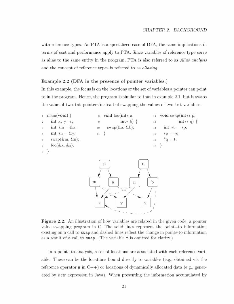
Example 2.2 (DFA in the presence of pointer variables.)
In this example, the focus is on the locations or the set of variables a pointer can point
to in the program. Hence, the program is similar to that in example 2.1, but it swaps
the value of two int pointers instead of swapping the values of two int variables.
1 main(void) {2 int x, y, z;3 int ∗m = &x;4 int ∗n = &y;5 swap(&m, &n);6 foo(&x, &z);7 }
8 void foo(int∗ a,9 int∗ b) {
10 swap(&a, &b);11 }
12 void swap(int∗∗ p,13 int∗∗ q) {14 int ∗t = ∗p;15 ∗p = ∗q;16 *q = t;17 }
z
am n
y
b
x
p q
Figure 2.2: An illustration of how variables are related in the given code, a pointervalue swapping program in C. The solid lines represent the points-to informationexisting on a call to swap and dashed lines reflect the change in points-to informationas a result of a call to swap. (The variable t is omitted for clarity.)
In a points-to analysis, a set of locations are associated with each reference vari-
able. These can be the locations bound directly to variables (e.g., obtained via the
reference operator & in C++) or locations of dynamically allocated data (e.g., gener-
ated by new expression in Java). When presenting the information accumulated by
21
CHAPTER 2. BACKGROUND
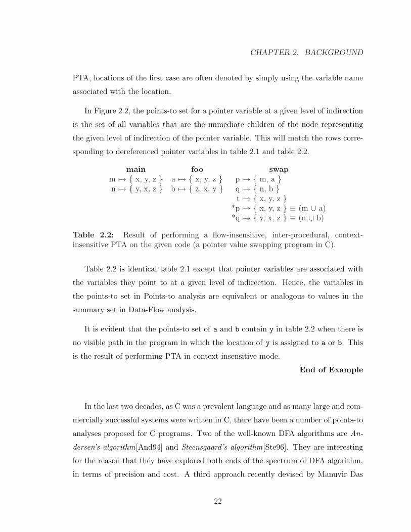
PTA, locations of the first case are often denoted by simply using the variable name
associated with the location.
In Figure 2.2, the points-to set for a pointer variable at a given level of indirection
is the set of all variables that are the immediate children of the node representing
the given level of indirection of the pointer variable. This will match the rows corre-
sponding to dereferenced pointer variables in table 2.1 and table 2.2.
main foo swapm 7→ { x, y, z } a 7→ { x, y, z } p 7→ { m, a }n 7→ { y, x, z } b 7→ { z, x, y } q 7→ { n, b }
t 7→ { x, y, z }*p 7→ { x, y, z } ≡ (m ∪ a)*q 7→ { y, x, z } ≡ (n ∪ b)
Table 2.2: Result of performing a flow-insensitive, inter-procedural, context-insensitive PTA on the given code (a pointer value swapping program in C).
Table 2.2 is identical table 2.1 except that pointer variables are associated with
the variables they point to at a given level of indirection. Hence, the variables in
the points-to set in Points-to analysis are equivalent or analogous to values in the
summary set in Data-Flow analysis.
It is evident that the points-to set of a and b contain y in table 2.2 when there is
no visible path in the program in which the location of y is assigned to a or b. This
is the result of performing PTA in context-insensitive mode.
End of Example
In the last two decades, as C was a prevalent language and as many large and com-
mercially successful systems were written in C, there have been a number of points-to
analyses proposed for C programs. Two of the well-known DFA algorithms are An-
dersen’s algorithm[And94] and Steensgaard’s algorithm[Ste96]. They are interesting
for the reason that they have explored both ends of the spectrum of DFA algorithm,
in terms of precision and cost. A third approach recently devised by Manuvir Das
22
CHAPTER 2. BACKGROUND
is interesting because it blends the above mentioned algorithms to obtain reasonable
precision and improved scalability. We summarize the main ideas of each of these
below.
2.2.1 Andersen’s Algorithm
Lars Ole Andersen described a Pointer Analysis for C programming language in his
PhD Thesis[And94]. The main characteristics of this algorithm are that it is very
precise, but expensive in terms of performance compared to other popular approaches.
According to this algorithm, a pointer-to-pointer assignment is to be treated as
unidirectional (in the direction of the assignment) to calculate the points-to infor-
mation, i.e., in pointer-to-pointer assignments, like dest = src where dest and src
are distinct pointer variables, after the assignment dest can point to the location(s)
pointed to by src and the location(s) to which src can point to does not change.
Figure 2.2 is an close representation of the how pointer variables are related in
the source code given in example 2.2 when this algorithm is used.
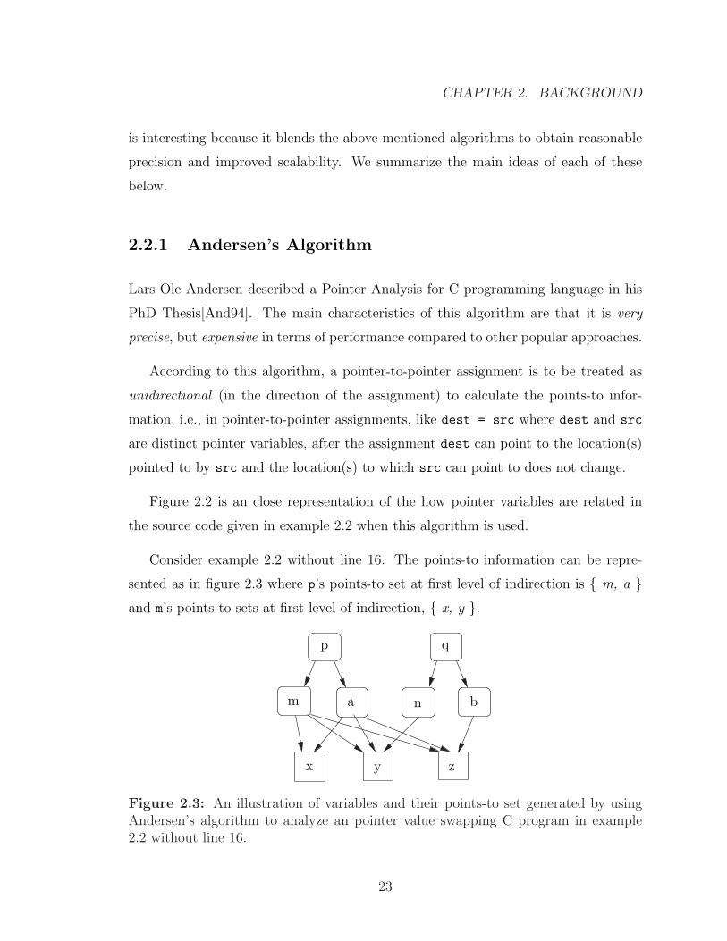
Consider example 2.2 without line 16. The points-to information can be repre-
sented as in figure 2.3 where p’s points-to set at first level of indirection is { m, a }and m’s points-to sets at first level of indirection, { x, y }.
z
am n
y
b
x
p q
Figure 2.3: An illustration of variables and their points-to set generated by usingAndersen’s algorithm to analyze an pointer value swapping C program in example2.2 without line 16.
23
CHAPTER 2. BACKGROUND
In the source code in example 2.2, as a result of the assignment at line 15 the values
in the points-to set of *q should be added to the points-to set of *p. As dereference
expressions do not have any points-to set and the assignment to expressions like *p is
actually the assignment to variables pointed to by p, i.e., m and a, it would suffice to
consider that there is a set of points-to sets associated with expressions like *p and an
assignment to *p would alter all the associated points-to sets. Hence, the assignment
will result in adding the values in all the points-to sets associated with *q to all the
points-to sets associated with *p.
Given the points-to sets associated with *q and *p, values from points-to sets
associated with *q may be added to points-to sets associated with *p even though
this is impossible at run-time. For example, it is clear from the program that m
cannot point to z at any point in the program, but the points-to information given
in figure 2.3 indicates that m will point to z.
To calculate such information, each pointer variable is associated with a points-
to set. This will result in the most precise information in terms of the exact set of
locations a pointer can point to at different levels of indirection. On the other hand, it
will prove costly, both in terms of time and space, to maintain large number of small
points-to sets. However the precision of the information calculated by this algorithm
can be improved by applying it in flow, context, and/or thread sensitive modes as
described in section 2.1.
2.2.2 Steensgaard’s Algorithm
Bjarne Steensgaard described an imprecise but faster algorithm for points-to analysis
in [Ste96].
In this algorithm, any pointer-to-pointer assignments were considered as bidirec-
tional, i.e., in pointer-to-pointer assignments, like dest = src where dest and src
are pointer variables, after the assignment, the points-to set of both dest and src is
the union of the points-to sets of dest and src before the assignment. This collapses
24
CHAPTER 2. BACKGROUND
points-to sets as pointers are equated and hence improves the performance of the
PTA as the cost to manage fewer but larger points-to set is less both in terms of time
and space. On the other hand, the results from such points-to set is imprecise due to
the bidirectional nature of pointer assignments.
x, y, z
m, a n, b
qp
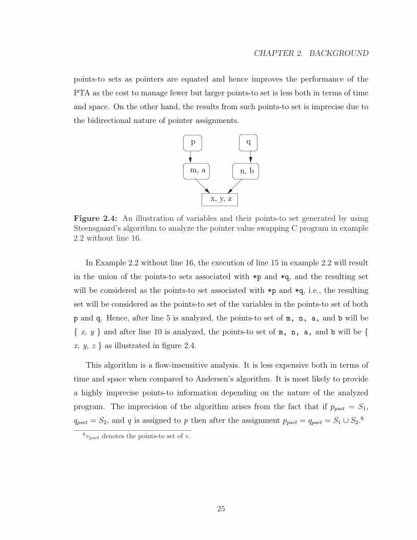
Figure 2.4: An illustration of variables and their points-to set generated by usingSteensgaard’s algorithm to analyze the pointer value swapping C program in example2.2 without line 16.
In Example 2.2 without line 16, the execution of line 15 in example 2.2 will result
in the union of the points-to sets associated with *p and *q, and the resulting set
will be considered as the points-to set associated with *p and *q, i.e., the resulting
set will be considered as the points-to set of the variables in the points-to set of both
p and q. Hence, after line 5 is analyzed, the points-to set of m, n, a, and b will be
{ x, y } and after line 10 is analyzed, the points-to set of m, n, a, and b will be {x, y, z } as illustrated in figure 2.4.
This algorithm is a flow-insensitive analysis. It is less expensive both in terms of
time and space when compared to Andersen’s algorithm. It is most likely to provide
a highly imprecise points-to information depending on the nature of the analyzed
program. The imprecision of the algorithm arises from the fact that if ppset = S1,
qpset = S2, and q is assigned to p then after the assignment ppset = qpset = S1 ∪ S2.6
6vpset denotes the points-to set of v.
25
CHAPTER 2. BACKGROUND
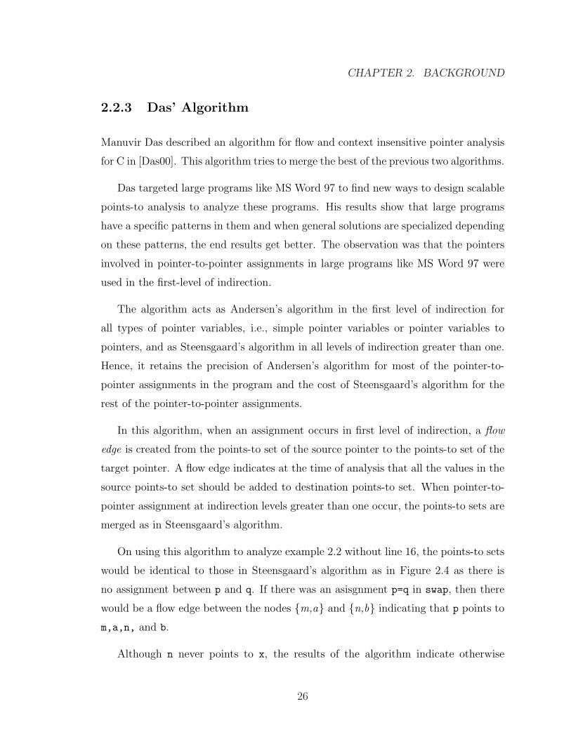
2.2.3 Das’ Algorithm
Manuvir Das described an algorithm for flow and context insensitive pointer analysis
for C in [Das00]. This algorithm tries to merge the best of the previous two algorithms.
Das targeted large programs like MS Word 97 to find new ways to design scalable
points-to analysis to analyze these programs. His results show that large programs
have a specific patterns in them and when general solutions are specialized depending
on these patterns, the end results get better. The observation was that the pointers
involved in pointer-to-pointer assignments in large programs like MS Word 97 were
used in the first-level of indirection.
The algorithm acts as Andersen’s algorithm in the first level of indirection for
all types of pointer variables, i.e., simple pointer variables or pointer variables to
pointers, and as Steensgaard’s algorithm in all levels of indirection greater than one.
Hence, it retains the precision of Andersen’s algorithm for most of the pointer-to-
pointer assignments in the program and the cost of Steensgaard’s algorithm for the
rest of the pointer-to-pointer assignments.
In this algorithm, when an assignment occurs in first level of indirection, a flow
edge is created from the points-to set of the source pointer to the points-to set of the
target pointer. A flow edge indicates at the time of analysis that all the values in the
source points-to set should be added to destination points-to set. When pointer-to-
pointer assignment at indirection levels greater than one occur, the points-to sets are
merged as in Steensgaard’s algorithm.
On using this algorithm to analyze example 2.2 without line 16, the points-to sets
would be identical to those in Steensgaard’s algorithm as in Figure 2.4 as there is
no assignment between p and q. If there was an asisgnment p=q in swap, then there
would be a flow edge between the nodes {m,a} and {n,b} indicating that p points to
m,a,n, and b.
Although n never points to x, the results of the algorithm indicate otherwise
26
CHAPTER 2. BACKGROUND
(similar to Steensgaard’s algorithm) as Das’ algorithm merges points-to sets at levels
of indirection greater than one. Hence, the precision of this algorithm will be less
when compared to that of Andersen’s algorithm. On the other hand, the summary
sets associated with p and q are similar to that obtained in Andersen’s algorithm and
better than those calculated by Steensgaard’s algorithm. Hence, the precision of this
algorithm is higher than that of Steensgaard’s algorithm.
2.2.4 Liang’s Algorithm
Donglin Liang proposed a flow-insensitive and context-sensitive points-to analysis for
C in [LH99]. This algorithm is modular, multi-phased and uses approaches from
Steensgaard’s algorithm in one of three phase.
In the phase 1, points-to graph is created for each procedure in the system being
analyzed. This points-to graph will only consider only non-global variables. Hence,
at the end of phase 1 there will be numerous procedure-local points-to graphs.
In phase 2, two activities occur. One is the construction of the points-to graph in-
volving global variables from the information available from all procedure-local points-
to graph. In the other activity local alias information in the callees is propogated
to their callers till the points-to graph for the procedures stabilize. This leads to
the processing of procedures in reverse topological order. This is one of the key to
achieving context-sensitive analysis.
The analysis continues to build the global variable points-to graph while propogat-
ing the alias information from the caller procedures to the callee procedure in phase
3. Here again, the procedures are processed till the points-to graph for the procedures
stabilize. In this phase, the procedures are processed in topological order.
As the alias information local to the callee is propogated to the caller before
propogating the alias information local to the caller to the callee, information is never
propogated along invalid call/return sequences. Also, both phases, 2 and 3, process
27

CHAPTER 2. BACKGROUND
procedures that appear as/in the strongly connected component of the call-graph.
Hence, context-sensitivity is achieved in the analysis.
qp
qp
qp
nm
nm
nm
x y
a
a
a
caller to calleeinfo from
Propogate points−to
Propogate points−toinfo from
callee to caller
graph constructionLocal points−to
Phase 3
Phase 2
Phase 1
m, a n, b
x, y, z
x, y
x, y
b
b
b
x, z
Figure 2.5: An illustration of Liang’s algorithm in various phases when applied tothe pointer value swapping C program given in example 2.2.
The final points-to information after phase 3 in figure 2.5 is more precise than
that in figure 2.3 (on page 21) as the points-to set for single-level indirection pointer
variables (m, n, a, and b) are more precise as a result of context sensitivity of the
analysis.
28
CHAPTER 2. BACKGROUND
2.3 Inter-Procedural Analysis
Intra-procedural analysis operates under worst-case assumptions as there is a lack of
information about the arguments to the procedure and the return value at a call-site.
This situation does not enable good optimization as the information in the callee
(caller) cannot be utilized in the caller (callee).
In the previous sections we illustrated how caller information can be used in the
callee. This was done by “binding” the arguments at each call-site to the parameters
of the procedure. Without such bindings, the summary-sets of say variables p and q
would be less interesting as they would not contain concrete values (probably abstract
values), and hence the resulting information will be imprecise.
Inter-Procedural Analysis is an analysis that spans across procedures (in terms
of data or control or both). The information obtained from such an analysis sub-
sumes the information obtained by performing intra-procedural analysis on the same
system. David Paul Grove’s PhD Thesis[Gro98] contains an excellent discussion of
inter-procedural analysis in the context of object-oriented languages.
In simple words, inter-procedural analysis can be viewed as performing intra-
procedural analysis of a given set of procedures and all “reachable” procedures by
considering the available information about/in the callee (caller) procedures in the
caller (callee) procedure. A procedure X is “reachable” from a procedure Y if a call
to X will be encountered by following a calling sequence emanating in Y. An analysis
that provides such “reachability” information is termed as reachability analysis. The
same concept is applicable to data.
In the context of inter-procedural analysis, to analyze a system there needs to be
one-level reachability information pertaining to procedures, i.e., all procedures called
(immediately reachable from) in a given procedure. This information is captured by
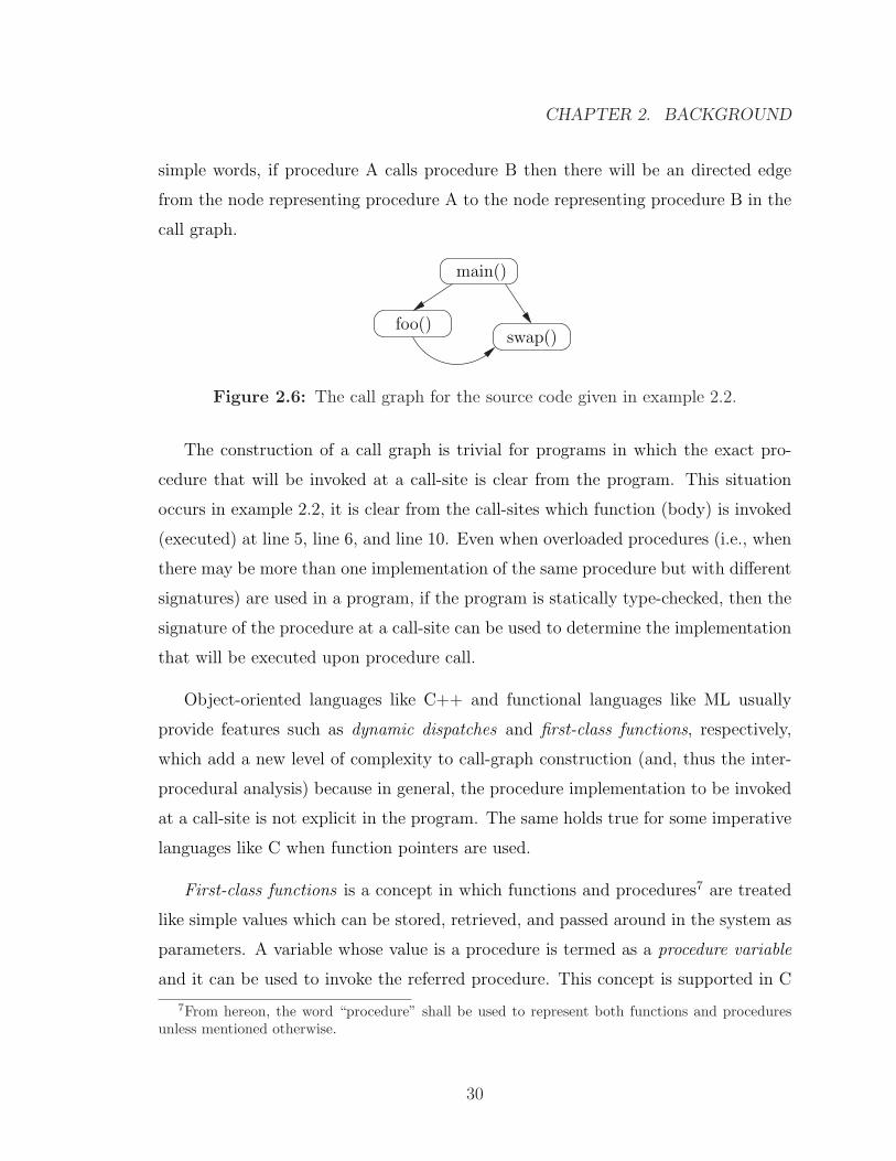
the call graph of the system. Call graph (figure 2.6) is a graph in which nodes represent
procedures and edges represent the reachability information between procedures. In
29
CHAPTER 2. BACKGROUND
simple words, if procedure A calls procedure B then there will be an directed edge
from the node representing procedure A to the node representing procedure B in the
call graph.
main()
swap()foo()
Figure 2.6: The call graph for the source code given in example 2.2.
The construction of a call graph is trivial for programs in which the exact pro-
cedure that will be invoked at a call-site is clear from the program. This situation
occurs in example 2.2, it is clear from the call-sites which function (body) is invoked
(executed) at line 5, line 6, and line 10. Even when overloaded procedures (i.e., when
there may be more than one implementation of the same procedure but with different
signatures) are used in a program, if the program is statically type-checked, then the
signature of the procedure at a call-site can be used to determine the implementation
that will be executed upon procedure call.
Object-oriented languages like C++ and functional languages like ML usually
provide features such as dynamic dispatches and first-class functions, respectively,
which add a new level of complexity to call-graph construction (and, thus the inter-
procedural analysis) because in general, the procedure implementation to be invoked
at a call-site is not explicit in the program. The same holds true for some imperative
languages like C when function pointers are used.
First-class functions is a concept in which functions and procedures7 are treated
like simple values which can be stored, retrieved, and passed around in the system as
parameters. A variable whose value is a procedure is termed as a procedure variable
and it can be used to invoke the referred procedure. This concept is supported in C
7From hereon, the word “procedure” shall be used to represent both functions and proceduresunless mentioned otherwise.
30
CHAPTER 2. BACKGROUND
and C++ via function pointers whereas languages like ML and Python8 support this
concept more naturally by considering each function definition as a value definition.
This concept in C is used extensively in the implementation of operating systems like
Linux9.
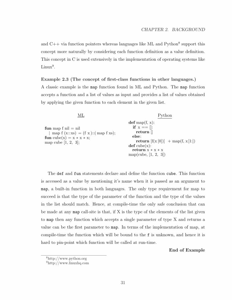
Example 2.3 (The concept of first-class functions in other languages.)
A classic example is the map function found in ML and Python. The map function
accepts a function and a list of values as input and provides a list of values obtained
by applying the given function to each element in the given list.
ML
fun map f nil = nil| map f (x::xs) = (f x )::( map f xs);
fun cube(x) = x ∗ x ∗ x;map cube [1, 2, 3];
Python
def map(f, x):if x == []:
return []else:
return [f(x [0])] + map(f, x[1:])def cube(x):
return x ∗ x ∗ xmap(cube, [1, 2, 3])
The def and fun statements declare and define the function cube. This function
is accessed as a value by mentioning it’s name when it is passed as an argument to
map, a built-in function in both languages. The only type requirement for map to
succeed is that the type of the parameter of the function and the type of the values
in the list should match. Hence, at compile-time the only safe conclusion that can
be made at any map call-site is that, if X is the type of the elements of the list given
to map then any function which accepts a single parameter of type X and returns a
value can be the first parameter to map. In terms of the implementation of map, at
compile-time the function which will be bound to the f is unknown, and hence it is
hard to pin-point which function will be called at run-time.
End of Example
8http://www.python.org9http://www.linuxhq.com
31
CHAPTER 2. BACKGROUND
Dynamic dispatch, as described in section 1.310, is a concept in object-oriented
technology in which the method to be invoked on a variable is determined by the
class or the type of the object to which that variable is bound to at the time of
method invocation during run-time. This is similar to first-class functions in that
there is more than one function that can be invoked at a call-site and in general,
the particular function to call cannot be determined until run-time. The object to
which the variable is bound to at invocation time is called as receiver object11 or
simply receiver. Dynamic dispatch is supported in object-oriented languages through
a mixture of inheritance, method overriding, and reference types. It is used exten-
sively in languages like C++, Java, and Python to realize patterns and frameworks.
GUI frameworks like wxGTK (wxWindows implementation on GTK (GIMP Tool
Kit)), MFC (Microsoft Foundation Classes), JFC (Java Foundation Classes), and
PMW (Python Mega-Widgets), and Communication frameworks like AC E(Adaptive
Communication Framework).
One approximate way to solve this issue is by using static type information. In
this case, at a call-site, all the possible method implementation that can be invoked
depending on the static type of the receiver variable is determined. If the static type
of the receiver variable is X, then the number of method implementations that will be
considered at the call-site will depend on the number of method implementation for
the method signature available in the subtypes of X. Usually, this number decreases
with the distance between X and the dynamic type in the type hierarchy.
In call graphs of systems written in languages that support first-class functions,
each call-site at which first-class functions are used will result in multiple directed
edges wherein the destination of the edge will be nodes corresponding to different
procedures that can possibly be invoked at that call-site. This is also true in case of
object-oriented languages at virtual method invocation sites.
When first-class functions and dynamic dispatches are considered, the precision of
10Refer to example 1.1 for an example.11In both, first-class functions and dynamic dispatch, the procedure name is bound to the imple-
mentation at run-time. Such binding is termed as dynamic-binding or late-binding.
32
CHAPTER 2. BACKGROUND
procedure implementationreceiver classes /
call graph construction
inter-procedural analysis
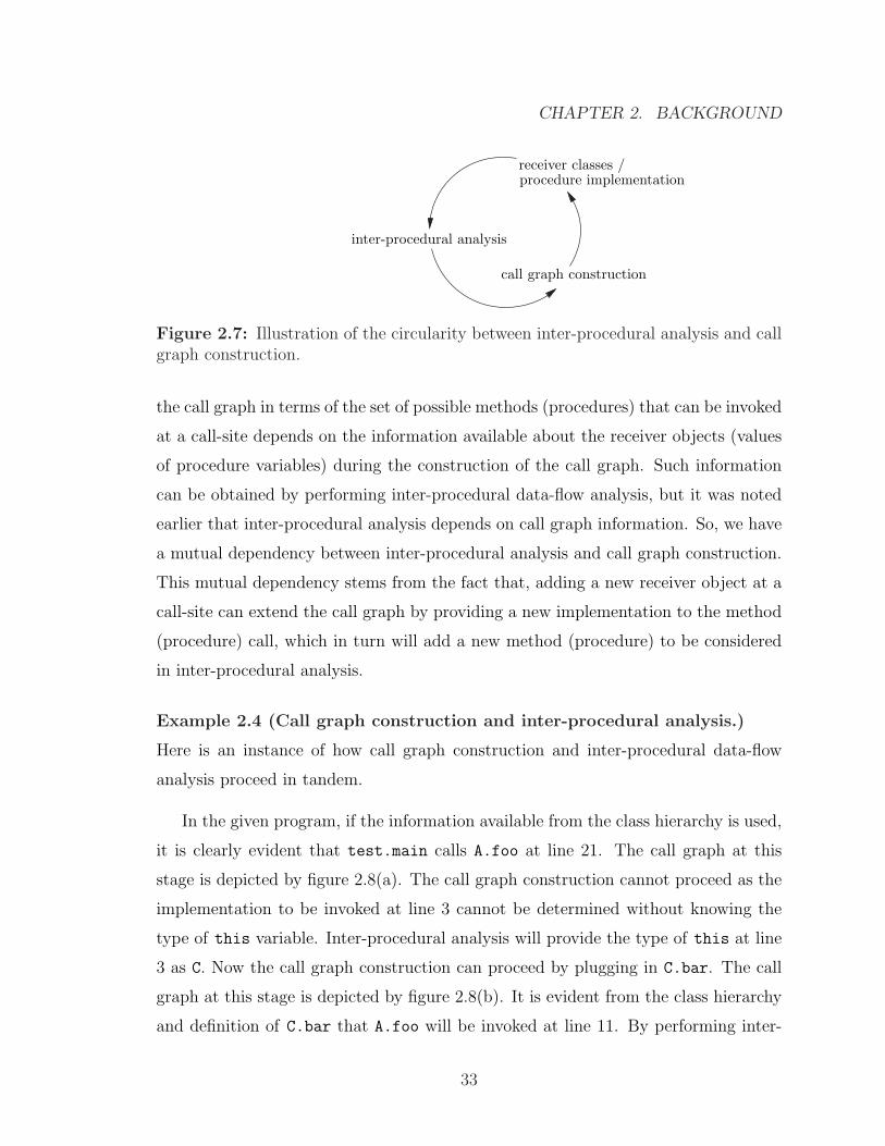
Figure 2.7: Illustration of the circularity between inter-procedural analysis and callgraph construction.
the call graph in terms of the set of possible methods (procedures) that can be invoked
at a call-site depends on the information available about the receiver objects (values
of procedure variables) during the construction of the call graph. Such information
can be obtained by performing inter-procedural data-flow analysis, but it was noted
earlier that inter-procedural analysis depends on call graph information. So, we have
a mutual dependency between inter-procedural analysis and call graph construction.
This mutual dependency stems from the fact that, adding a new receiver object at a
call-site can extend the call graph by providing a new implementation to the method
(procedure) call, which in turn will add a new method (procedure) to be considered
in inter-procedural analysis.
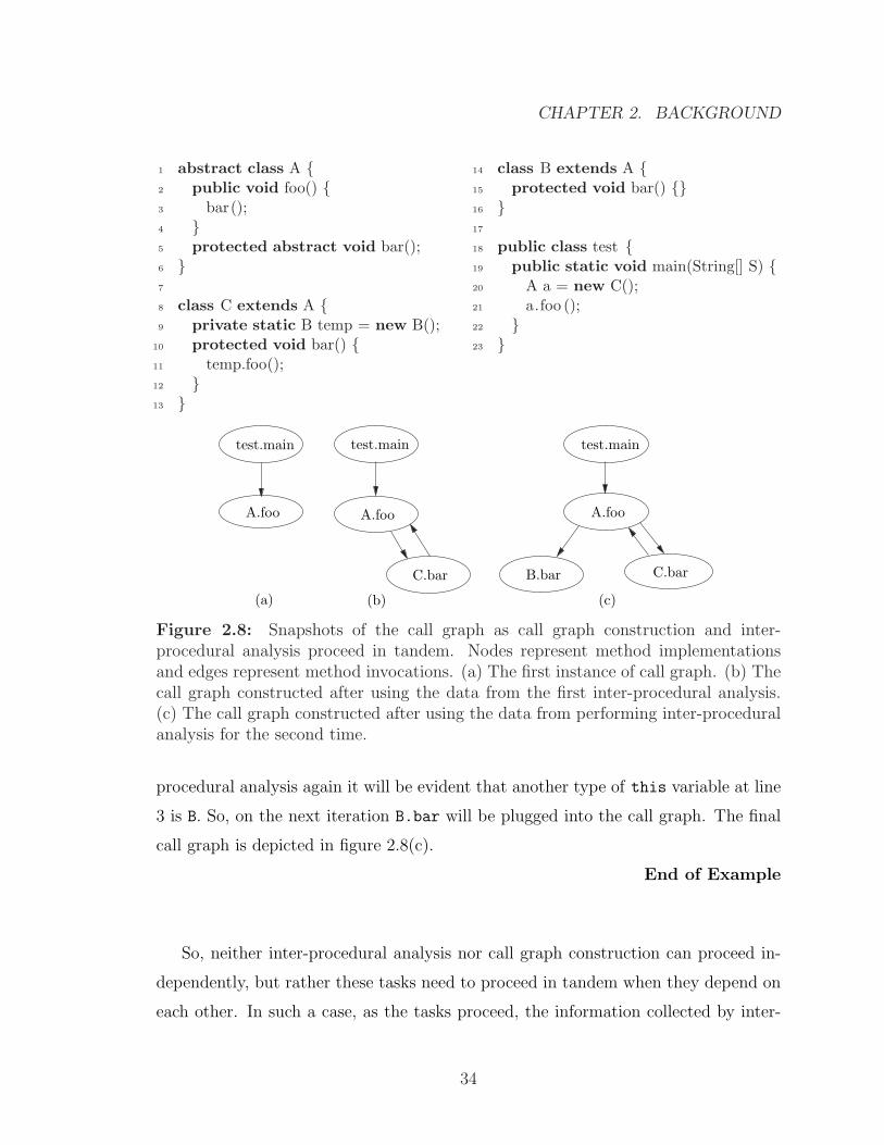
Example 2.4 (Call graph construction and inter-procedural analysis.)
Here is an instance of how call graph construction and inter-procedural data-flow
analysis proceed in tandem.
In the given program, if the information available from the class hierarchy is used,
it is clearly evident that test.main calls A.foo at line 21. The call graph at this
stage is depicted by figure 2.8(a). The call graph construction cannot proceed as the
implementation to be invoked at line 3 cannot be determined without knowing the
type of this variable. Inter-procedural analysis will provide the type of this at line
3 as C. Now the call graph construction can proceed by plugging in C.bar. The call
graph at this stage is depicted by figure 2.8(b). It is evident from the class hierarchy
and definition of C.bar that A.foo will be invoked at line 11. By performing inter-
33
CHAPTER 2. BACKGROUND
1 abstract class A {2 public void foo() {3 bar();4 }5 protected abstract void bar();6 }7
8 class C extends A {9 private static B temp = new B();
10 protected void bar() {11 temp.foo();12 }13 }
14 class B extends A {15 protected void bar() {}16 }17
18 public class test {19 public static void main(String[] S) {20 A a = new C();21 a.foo ();22 }23 }
A.foo
test.main
(a)
A.foo
test.main
C.bar
(b)
B.bar
A.foo
test.main
C.bar
(c)
Figure 2.8: Snapshots of the call graph as call graph construction and inter-procedural analysis proceed in tandem. Nodes represent method implementationsand edges represent method invocations. (a) The first instance of call graph. (b) Thecall graph constructed after using the data from the first inter-procedural analysis.(c) The call graph constructed after using the data from performing inter-proceduralanalysis for the second time.
procedural analysis again it will be evident that another type of this variable at line
3 is B. So, on the next iteration B.bar will be plugged into the call graph. The final
call graph is depicted in figure 2.8(c).
End of Example
So, neither inter-procedural analysis nor call graph construction can proceed in-
dependently, but rather these tasks need to proceed in tandem when they depend on
each other. In such a case, as the tasks proceed, the information collected by inter-
34
CHAPTER 2. BACKGROUND
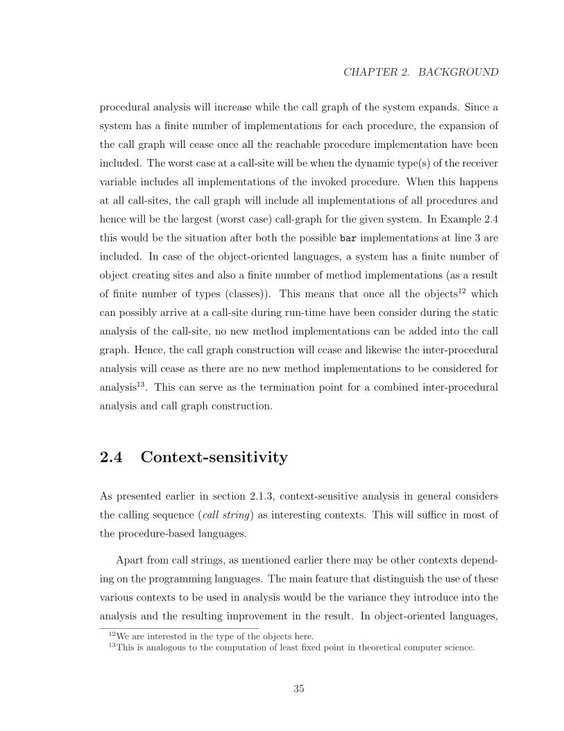
procedural analysis will increase while the call graph of the system expands. Since a
system has a finite number of implementations for each procedure, the expansion of
the call graph will cease once all the reachable procedure implementation have been
included. The worst case at a call-site will be when the dynamic type(s) of the receiver
variable includes all implementations of the invoked procedure. When this happens
at all call-sites, the call graph will include all implementations of all procedures and
hence will be the largest (worst case) call-graph for the given system. In Example 2.4
this would be the situation after both the possible bar implementations at line 3 are
included. In case of the object-oriented languages, a system has a finite number of
object creating sites and also a finite number of method implementations (as a result
of finite number of types (classes)). This means that once all the objects12 which
can possibly arrive at a call-site during run-time have been consider during the static
analysis of the call-site, no new method implementations can be added into the call
graph. Hence, the call graph construction will cease and likewise the inter-procedural
analysis will cease as there are no new method implementations to be considered for
analysis13. This can serve as the termination point for a combined inter-procedural
analysis and call graph construction.
2.4 Context-sensitivity
As presented earlier in section 2.1.3, context-sensitive analysis in general considers
the calling sequence (call string) as interesting contexts. This will suffice in most of
the procedure-based languages.
Apart from call strings, as mentioned earlier there may be other contexts depend-
ing on the programming languages. The main feature that distinguish the use of these
various contexts to be used in analysis would be the variance they introduce into the
analysis and the resulting improvement in the result. In object-oriented languages,
12We are interested in the type of the objects here.13This is analogous to the computation of least fixed point in theoretical computer science.
35
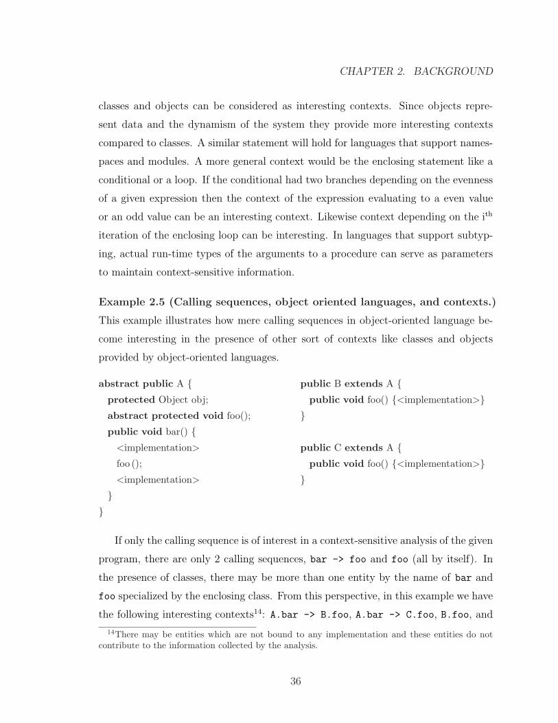
CHAPTER 2. BACKGROUND
classes and objects can be considered as interesting contexts. Since objects repre-
sent data and the dynamism of the system they provide more interesting contexts
compared to classes. A similar statement will hold for languages that support names-
paces and modules. A more general context would be the enclosing statement like a
conditional or a loop. If the conditional had two branches depending on the evenness
of a given expression then the context of the expression evaluating to a even value
or an odd value can be an interesting context. Likewise context depending on the ith
iteration of the enclosing loop can be interesting. In languages that support subtyp-
ing, actual run-time types of the arguments to a procedure can serve as parameters
to maintain context-sensitive information.
Example 2.5 (Calling sequences, object oriented languages, and contexts.)
This example illustrates how mere calling sequences in object-oriented language be-
come interesting in the presence of other sort of contexts like classes and objects
provided by object-oriented languages.
abstract public A {protected Object obj;
abstract protected void foo();
public void bar() {<implementation>
foo ();
<implementation>
}}
public B extends A {public void foo() {<implementation>}}
public C extends A {public void foo() {<implementation>}}
If only the calling sequence is of interest in a context-sensitive analysis of the given
program, there are only 2 calling sequences, bar -> foo and foo (all by itself). In
the presence of classes, there may be more than one entity by the name of bar and
foo specialized by the enclosing class. From this perspective, in this example we have
the following interesting contexts14: A.bar -> B.foo, A.bar -> C.foo, B.foo, and
14There may be entities which are not bound to any implementation and these entities do notcontribute to the information collected by the analysis.
36
CHAPTER 2. BACKGROUND
C.foo. These context bear more influence on the analysis when data is defined at a
class level using static modifier in Java.
In case the reference variable obj declared in A is used in foo then it makes sense
to consider the instance as defined in the enclosing context, class B or class C, to
improve the precision of the analysis. Hence, classes in object-oriented languages are
indeed interesting to be considered as contexts. On the other hand, if fully qualified
names are used at (static) member access and method invocation sites then the same
precision achieved by considering classes as context is achieved.
The same idea can be extended to objects, but not as is. Ideally, objects represent
data and capture the dynamism of the system, and classes represent control and
capture the static-ness of the system. Hence, when considering member variables it
would make the analysis more precise if the information pertaining to the member
variable is specific to the enclosing object. This comes close to static execution of
programs.
End of Example
Refining the definition presented in section 2.4, a context may be any semantic
device (construct) which can influence the result of execution of the code as described
previously. Hence, the context can be parameterized by the following parameters in
an analysis that is context-sensitive.
- Nature of the constituents of the context. This may be the calling sequence as
in imperative and functional languages. In case of object-oriented languages,
the constituents may include classes and objects.
- Number of constituents in the context. This will be the length of call stack
in case of imperative and functional languages. In case of object-oriented lan-
guages, this may also include the number of enclosing classes and objects.
Although information obtained by taking into consideration all these factors will
37
CHAPTER 2. BACKGROUND
nonetheless be invaluable, but at the same time it will be very expensive to compute
such information. The real issue is how the space and time complexity of the process
that computes such information compares to that of the process that consumes such
information. Also how relevant or important is the information of this nature. At
present, the complexity of the computation process is relatively high compared to
that of consumption process, and so the on-going research is to reduce this cost gap.
As the cost per unit of computing power decreases and the need for such informa-
tion increases in much complex processes such as model extraction for the purpose
of model checking, the use of context-sensitive inter-procedural analysis will become
prevalent.
2.5 Java
It’s been ten years since Java entered the market as a programming language and
it has been accepted and adopted by the software community to an extent that it
surpasses the acceptance and adoption of C or C++ by the same community.
The creator(s) of Java did a great job in learning from the mistakes of C++
(pointers) and not repeating them again. At the same time they cleanly integrated
features into Java such as reference types, interfaces, and packages. The one feature
that was a major cause for it’s acceptance was “Write Once, Run Anywhere(WORA)”.
This was not a new feature, but rather one that was tried and tested in IBM 370.
The idea was to compile the source code to be executed by Java Virtual Machine
(JVM). JVM is implemented in software similar to an i386 simulator on a SPARC
machine. So once the software is written in Java and compiled to run on a JVM, it
can be run on any platform where the JVM is available. Hence, the end result was an
object-oriented language which was clean, simple, rich with features, and advocated
and practiced “WORA”15.
15As the language has evolved, “WORA” feature has become debatable.
38
CHAPTER 2. BACKGROUND
Like C, because of the huge acceptance and prevalent use of Java in the software
industry the number of on-going research projects related to Java is high. Among
these, quite a few are related to automatic verification of Java programs. The moti-
vations for these projects are
- the computational power required by automated verification is not prohibitive
as the cost per unit of computing power has been decreasing,
- ever increasing complexity of the systems,
- Java being considered to program safety critical systems, and
- formal methods reaching a level of maturity required by the software industry.
The catch is that model checking can be used verify properties of systems written
in Java as being realized in the on-going Bandera[CDH+00] project at Kansas State
University.
Java supports a rich set of primitive data types and operations on them. This
implies that the effect of these data types on the model of the system needs to be
controlled. This is achieved by data abstraction. A simple example would be the use of
Signs abstraction to abstract an integer variable based on the polarity of it’s value as
described on page 4. When these new data types occur in conditional expressions, new
paths that did not exist before may be injected into the model and a non-deterministic
choice will be made over these paths. The number of newly injected paths will usually
be less than the number that would have occurred if modeled without abstraction.
2.5.1 Data-Flow Analysis
Program slicing and other techniques like in-lining used during model extraction can
benefit from the information collected by data-flow analysis and object-flow analysis
in particular. The data-flow analyses possible on a Java program can be divided
depending on the types of data supported in Java:
39
CHAPTER 2. BACKGROUND
Simple Data Types
Data-Flow analysis of Java programs suffers from the large domain of values corre-
sponding to most of the simple data types. Hence, it is hard to design feasible and
tractable analysis that can provide information such as the set of possible concrete
values an integer variable can evaluate to. Rather feasible and tractable analyses
which gather information about “zero-ness”, non-null-ness, and such other properties
of primitive types can be devised. This is a hurdle faced when modeling systems
written in any programming languages supporting such simple data types.
Reference Types
Java supports inheritance, polymorphism, and reference types. As mentioned before
these are the required ingredients for dynamic dispatch which is supported in Java.
Hence, when a model needs to be extracted from a Java program, extraneous methods
which will not be invoked at the dynamic dispatch site are still considered at the site.
As a result, the size and complexity of the model blows up. If the information about
the type of the receiver is available beforehand, only the possible methods can be
modeled and hence the state-space of the model can be reduced. This information
can be inferred from the summary set of a reference variable on which the method
is dispatched. Such information can be obtained from performing a inter-procedural
data-flow analysis where objects are the values of interest. In simple words, a inter-
procedural points-to analysis on reference types will provide the required information.
The implications of lack of pointers and availability of reference types in Java
should be clear before discussing analyses related to references in Java. One of the
salient features of Java is that it does not support pointers, but supports reference
types as in C++16. In the presence of pointers, there can be more than one level on
indirection whereas this is not possible with reference types. Some may argue that a
16“Can the semantic effect of pointers be simulated with the support for reference types and dataencapsulation (through objects)?” is an interesting topic for debate.
40
CHAPTER 2. BACKGROUND
chain of member access over reference types like a.b.c is similar to a chain of pointer
dereferences like a->b->c. This is true as the level of indirection is one in both the
cases. In case of multiple levels of indirection, there is no equivalence as a.a.a is
equivalent to a->a->a and not ***a. So, at first level of indirection both pointer and
reference types can be used equivalently, but not at higher level of indirection even
with data encapsulation.
Now consider the previously discussed points-to analyses in the context of Java.
From the previous paragraph it follows immediately that Andersen’s and Das’ al-
gorithm will have the same precision when applied to a Java programs. On the
other hand Steensgaard’s algorithm will still be imprecise compared to the other two
algorithms.
In terms of the type of flow-analysis, flow-sensitive data-flow analysis or otherwise
in case of Java will not yield interestingly different result than when performed on C
or C++ as it supports more or less the same sort of expressions and statements.
Context-sensitive flow analysis of Java programs will produce different results as
the context of classes17 and objects need to be considered depending on the precision
of the analysis. The presence of dynamic context in the form of objects and static
contexts in the form of classes makes the analysis interesting as the data in the
enclosing class and objects can affect the analysis. Also, the presence of nested classes
with access specifiers from Java 1.1 on wards makes context-sensitive analysis more
interesting as nested classes and their instances can access the data in the enclosing
class and their instances.
The presence of dynamic and static context leads to an interesting situation. The
analyses can collect information considering only classes as the distinguishing factor.
Or the analysis can consider the object allocation sites as a distinguishing factor.
Hence, a context-sensitive analysis for Java may be classified as static or dynamic
depending on the contexts that shall be considered. Of course, suitable trade-offs will
17Interfaces are a specific form of declaration of classes and so will not be mentioned separately.
41
CHAPTER 2. BACKGROUND
occur in terms of time, space, and precision of the analysis.
As Java supports multi-threading as a language feature as well as through a library
it is possible to have thread-sensitive or thread-insensitive analysis of Java programs.
The only problem being that, in Java the “link” between the method that starts a
thread and the method that actually is executed in the thread is not syntactically
explicit, but rather it is embedded in the semantics of start and run methods of
java.lang.Thread class. As in any design frameworks implemented using object-
oriented language, a similar situation as presented in case of threads occurs in JFC
(AWT and Swing).
Java supports various forms of Reference objects from version 1.2 on wards. If
reference objects are used then the points-to analysis analysis will have to operate in
a assumed environment where the assumptions are about how the reference objects
shall behave in various situations.
2.5.2 Control-Flow Analysis
Java supports for a system to be composed of classes where each of them can provide
an entry point into the system, i.e., each class can define a main method. It may be
the case that not all entry points are alike in terms of execution results and program
behavior. Hence, the call graphs constructed starting from various entry points may
not be alike in terms of structure or methods corresponding to nodes or both.
Another situation is where the software does not have a main method, i.e., none
of the classes in the software define main method. These are usually libraries and not
complete system. In such cases, there shall be classes which implement
java.lang.Runnable interface or extend java.lang.Thread class. The environment
in which the library is used will instantiate a class and execute the
java.lang.Thread.start or java.lang.Runnable.run to set the machinery into
motion. This is a situation similar to that with multiple main methods. If parts of
the library are parameterized (which is usually the case) then due to the lack of in-
42

CHAPTER 2. BACKGROUND
formation about the arguments it will be hard to perform precise and useful analysis
to gather data about the run-time behavior of the library.
43
Chapter 3
Object-Flow Analysis
This chapter starts with an example justifying the need for object-flow analysis. This
is followed by an detailed discussion about object-flow analysis and how the analysis
is achieved. The explanation proceeds at an abstract level dealing with Java inde-
pendent of any intermediate representation.
3.1 Overview
Object-Flow Analysis (OFA) can provide information regarding the possible objects
to which a reference variable will evaluate at a particular program point.
This information is invaluable to program transformations which work conser-
vatively on the syntactic structure and the static characteristics of the source code
when concepts such as aliasing, data encapsulation, inheritance, and polymorphism
are used in the source code. As described earlier, this information can help trans-
formations to be aggressive at dynamic dispatch sites. Likewise, when encapsulated
data is defined and used through aliases, the information from such an analysis can
be used to determine if the aliases correspond to the same object.
44
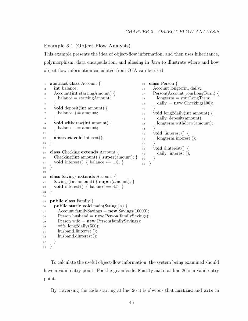
CHAPTER 3. OBJECT-FLOW ANALYSIS
Example 3.1 (Object Flow Analysis)
This example presents the idea of object-flow information, and then uses inheritance,
polymorphism, data encapsulation, and aliasing in Java to illustrate where and how
object-flow information calculated from OFA can be used.
1 abstract class Account {2 int balance;3 Account(int startingAmount) {4 balance = startingAmount;5 }6 void deposit(int amount) {7 balance += amount;8 }9 void withdraw(int amount) {
10 balance −= amount;11 }12 abstract void interest();13 }14
15 class Checking extends Account {16 Checking(int amount) { super(amount); }17 void interest () { balance ∗= 1.8; }18 }19
20 class Savings extends Account {21 Savings(int amount) { super(amount); }22 void interest () { balance ∗= 4.5; }23 }24
25 public class Family {26 public static void main(String[] s) {27 Account familySavings = new Savings(10000);28 Person husband = new Person(familySavings);29 Person wife = new Person(familySavings);30 wife . long2daily(500);31 husband.linterest ();32 husband.dinterest();33 }34 }
35 class Person {36 Account longterm, daily;37 Person(Account yourLongTerm) {38 longterm = yourLongTerm;39 daily = new Checking(100);40 }41 void long2daily(int amount) {42 daily .deposit(amount);43 longterm.withdraw(amount);44 }45 void linterest () {46 longterm. interest ();47 }48 void dinterest() {49 daily . interest ();50 }51 }
To calculate the useful object-flow information, the system being examined should
have a valid entry point. For the given code, Family.main at line 26 is a valid entry
point.
By traversing the code starting at line 26 it is obvious that husband and wife in
45
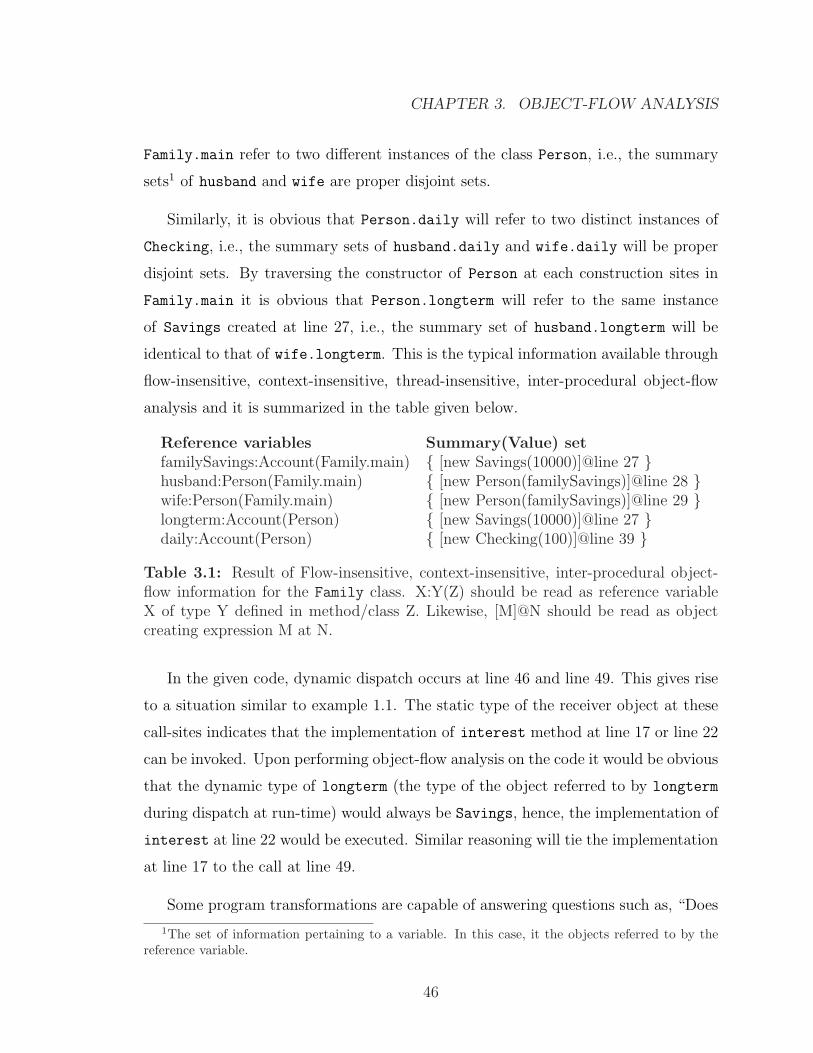
CHAPTER 3. OBJECT-FLOW ANALYSIS
Family.main refer to two different instances of the class Person, i.e., the summary
sets1 of husband and wife are proper disjoint sets.
Similarly, it is obvious that Person.daily will refer to two distinct instances of
Checking, i.e., the summary sets of husband.daily and wife.daily will be proper
disjoint sets. By traversing the constructor of Person at each construction sites in
Family.main it is obvious that Person.longterm will refer to the same instance
of Savings created at line 27, i.e., the summary set of husband.longterm will be
identical to that of wife.longterm. This is the typical information available through
flow-insensitive, context-insensitive, thread-insensitive, inter-procedural object-flow
analysis and it is summarized in the table given below.
Reference variables Summary(Value) setfamilySavings:Account(Family.main) { [new Savings(10000)]@line 27 }husband:Person(Family.main) { [new Person(familySavings)]@line 28 }wife:Person(Family.main) { [new Person(familySavings)]@line 29 }longterm:Account(Person) { [new Savings(10000)]@line 27 }daily:Account(Person) { [new Checking(100)]@line 39 }
Table 3.1: Result of Flow-insensitive, context-insensitive, inter-procedural object-flow information for the Family class. X:Y(Z) should be read as reference variableX of type Y defined in method/class Z. Likewise, [M]@N should be read as objectcreating expression M at N.
In the given code, dynamic dispatch occurs at line 46 and line 49. This gives rise
to a situation similar to example 1.1. The static type of the receiver object at these
call-sites indicates that the implementation of interest method at line 17 or line 22
can be invoked. Upon performing object-flow analysis on the code it would be obvious
that the dynamic type of longterm (the type of the object referred to by longterm
during dispatch at run-time) would always be Savings, hence, the implementation of
interest at line 22 would be executed. Similar reasoning will tie the implementation
at line 17 to the call at line 49.
Some program transformations are capable of answering questions such as, “Does
1The set of information pertaining to a variable. In this case, it the objects referred to by thereference variable.
46
CHAPTER 3. OBJECT-FLOW ANALYSIS
statement A affect the outcome of statement B?” A similar question that can be posed
on the given code is “Does statement at line 30 affect the outcome of the statement at
line 31?” Since the given statements contain method calls, it would be safe to assume
that, “if statements involved in the method call at line 30 affects any of the statements
involved in the method call at line 31, then statement at line 30 affects the statement
at line 31.” Without OFA it is impossible to answer this question as it is unknown
which implementation of interest will be invoked at line 46. Rather, it is possible to
answer the question by conservatively considering all possible implementations that
can be invoked at line 46, but this may prove rather imprecise.
However, on performing object-flow analysis it is possible to improve the precision.
Consider lines 30 and 32. These lines will involve line 17 and line 7. The summary
sets corresponding to this variables in the latter two lines are disjoint, hence, it safe
to infer that line 30 will not affect line 32.
If the same question is posed to lines line 30 and line 31, by the static type of
the receiver objects it is possible to conservatively infer that line 30 affects line 31.
The fact that the summary set for this variable at line 22 and line 10 has a common
element improves the confidence in the inference. However, this does not help in
“must” scenarios, but in “may-be” scenarios.
Hence, the information from object-flow analysis can be used to improve the pre-
cision of the results of program transformations. At the same time it can also be used
to verify the results of program transformations.
End of Example
As discussed in earlier chapters OFA can be instrumented to yield information of
varied amount of precision as per requirement, and the cost for calculating object-flow
information is directly proportional to the required precision. One such instrumen-
tation might be that instance variables belonging to different object have different
summary sets. In terms of the previous example this would mean that there shall be
47
CHAPTER 3. OBJECT-FLOW ANALYSIS
two instances of daily in object-flow information, one corresponding to the instance
of Person created at line 28 and another corresponding to the instance of Person
created at line 29. longterm will also be treated similarly. The only distinction being
that the summary sets of the dailys will be proper disjoint sets due to the adapted
partitioning of instance variables, but the summary sets of longterms will still be
identical sets. Although the difference in the result of OFA is subtle, such results
permit more specific queries which can significantly improve the precision of program
transformations.
3.2 Concept
This section shall present the basic terms of DFA and later on use them to describe
OFA. It is followed by the details of how flow analysis is achieved.
The concept of program point presented in section 2.1.1 will be used here. P shall
denote the set of program points in a given system, S. It is possible for a system to
have more than one entry point and/or more than one exit point. It is almost always
true that a system starts executing from a single program point. Also, if more than
one entry point is considered then more than one independent control and data flow
network may exist in the system at the same time which will worsen the problem.
On the other hand exit points do not influence the number of independent control
and data flow networks. Hence, it easy to view a system with multiple entry and exit
points to be a collection of variations of the given system with distinct entry point
but with all the exit points as in the given system.
If N ⊂ P and X ⊂ P are the set of entry and exit points, respectively, of a given
system, S, then S can be considered as a collection of systems, Si, such that
- ∀Si.|Ni| = 1,
- ∀Si.Xi ⊆ X, and
48
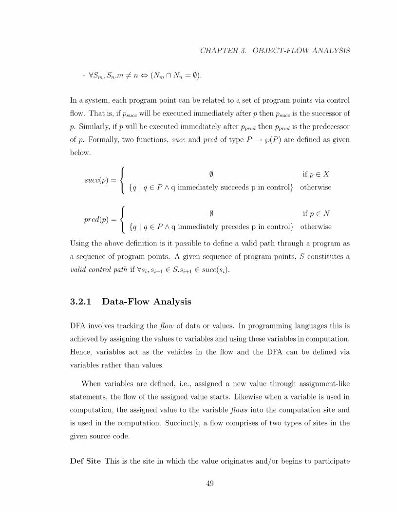
CHAPTER 3. OBJECT-FLOW ANALYSIS
- ∀Sm, Sn.m 6= n⇔ (Nm ∩Nn = ∅).
In a system, each program point can be related to a set of program points via control
flow. That is, if psucc will be executed immediately after p then psucc is the successor of
p. Similarly, if p will be executed immediately after ppred then ppred is the predecessor
of p. Formally, two functions, succ and pred of type P → ℘(P ) are defined as given
below.
succ(p) =
∅ if p ∈ X
{q | q ∈ P ∧ q immediately succeeds p in control} otherwise
pred(p) =
∅ if p ∈ N
{q | q ∈ P ∧ q immediately precedes p in control} otherwise
Using the above definition is it possible to define a valid path through a program as
a sequence of program points. A given sequence of program points, S constitutes a
valid control path if ∀si, si+1 ∈ S.si+1 ∈ succ(si).
3.2.1 Data-Flow Analysis
DFA involves tracking the flow of data or values. In programming languages this is
achieved by assigning the values to variables and using these variables in computation.
Hence, variables act as the vehicles in the flow and the DFA can be defined via
variables rather than values.
When variables are defined, i.e., assigned a new value through assignment-like
statements, the flow of the assigned value starts. Likewise when a variable is used in
computation, the assigned value to the variable flows into the computation site and
is used in the computation. Succinctly, a flow comprises of two types of sites in the
given source code.
Def Site This is the site in which the value originates and/or begins to participate
49
CHAPTER 3. OBJECT-FLOW ANALYSIS
in the flow by being assigned to a variable. In other words, it is any syn-
tactic construct in the programming language that “assigns to” or “defines” a
variable. In Java, this would comprise all variants of assignment expression-
statement, parameter-passing through method calls, and member variable dec-
larations (with and without initializations). For example, line 29 in example
3.1 is def site for the variable wife and Person.longterm.
Use Site This is the site in which the value is used in computation via the variable
to which it is assigned. In other words, it is any syntactic construct in the
programming language that “refers” or “uses” a variable in computation. In
Java this would be any site in the program where a variable used to obtain
associated value. Line 30 in example 3.1 is a use site for the variable wife.
In terms of this new vocabulary, a value starts the “flow” at a def site and flows
through all the program points along the flow path from the def site to any use site.
Hence, a flow path for a given variable is a sequence of program points from a def
site to a use site for the given variable, including both def and use site. Formally,
if d is a def site, u is a use site, and F = 〈d, p1, p2, . . . , pn, u〉 is valid control path,
then F is a flow path from d to u. This definition does not address the issue if any of
the pi is a def site for the given variable. If any such def site occurs then it is called
as intervening definition of the given variable between the given def and use site. A
more stricter definition of flow path would be, if d is a def site and u is a use site,
F = 〈d, p1, p2, . . . , pn, u〉 is valid control path, and none of the pi in F are def sites for
the given variable, then F is a flow path from d to u for the given variable. Any such
def site which has such a flow path to a use site is termed as reaching definition.
Likewise, an analysis in which the subject of the analysis is the flow of data as
described above, is a Data-Flow Analysis or Flow Analysis. Hence, an analysis which
will provide all the def and use sites for a given variable in the given source code is also
a DFA. By this definition it is also possible for the DFA to provide information such
as set of possible values a variable can evaluate in an expression. Such a set which
is associated with the variable and contains all the values a variable can evaluate
50
CHAPTER 3. OBJECT-FLOW ANALYSIS
to is called as Valueset or a Flowset of the given variable. Given a variable a, the
associated valueset would be denoted as Va. If the DFA uses information such as flow
path and in turn control-flow to determine the order in which def and use sites may be
encountered to provide information such as which def sites may influence an use site,
then such an analysis is a flow-sensitive DFA. Such a DFA is capable of providing a
value set of a variable corresponding to a given program point in a given source code,
i.e., the value set contains only the values the variables can evaluate to at the given
program point. As discussed previously such analysis can take the context and the
execution model into consideration to provide suitable information about the flow of
data in the system.
3.2.2 Object-Flow Analysis
In simple words, Object-Flow Analysis is data-flow analysis as described in the previ-
ous section in which the only data considered in the flow analysis are objects created
in the given system. Elaborately, an analysis in which
- the variables are of reference types, i.e., they evaluate to object references,
- the provided def sites and use sites involve reference variables, and
- the flow paths corresponds to the paths along which objects flow
can be termed as Object-Flow Analysis. Hence, the definitions in the previous section
needs to be refined as the value set is refined to include only objects.
The def sites in the context of OFA will be only assignment-like statements which
assign a (new) object to a variable. In Java, this would include any statement in
which a reference variable is assigned an object reference, i.e., analogous to l-value in
C/C++. This will include simple assignments to reference variables and assignments
via method calls.
51
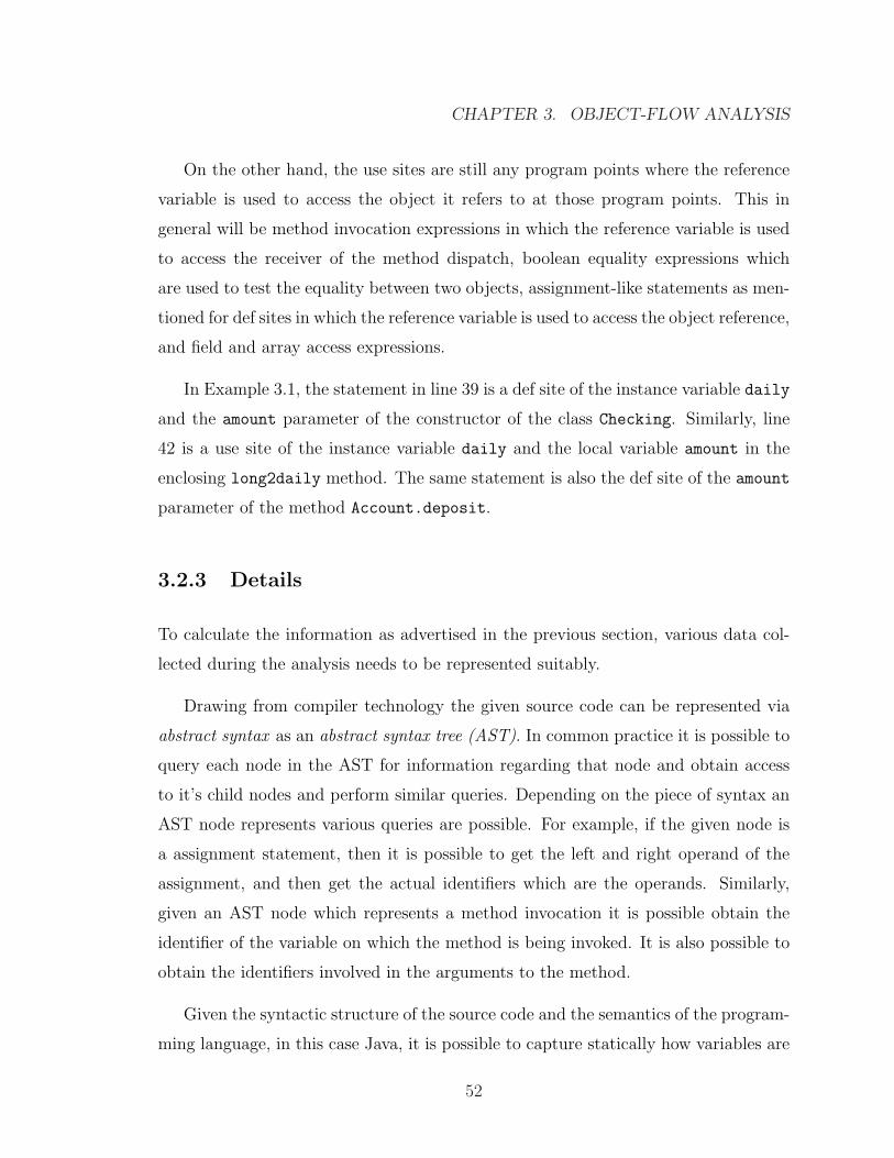
CHAPTER 3. OBJECT-FLOW ANALYSIS
On the other hand, the use sites are still any program points where the reference
variable is used to access the object it refers to at those program points. This in
general will be method invocation expressions in which the reference variable is used
to access the receiver of the method dispatch, boolean equality expressions which
are used to test the equality between two objects, assignment-like statements as men-
tioned for def sites in which the reference variable is used to access the object reference,
and field and array access expressions.
In Example 3.1, the statement in line 39 is a def site of the instance variable daily
and the amount parameter of the constructor of the class Checking. Similarly, line
42 is a use site of the instance variable daily and the local variable amount in the
enclosing long2daily method. The same statement is also the def site of the amount
parameter of the method Account.deposit.
3.2.3 Details
To calculate the information as advertised in the previous section, various data col-
lected during the analysis needs to be represented suitably.
Drawing from compiler technology the given source code can be represented via
abstract syntax as an abstract syntax tree (AST). In common practice it is possible to
query each node in the AST for information regarding that node and obtain access
to it’s child nodes and perform similar queries. Depending on the piece of syntax an
AST node represents various queries are possible. For example, if the given node is
a assignment statement, then it is possible to get the left and right operand of the
assignment, and then get the actual identifiers which are the operands. Similarly,
given an AST node which represents a method invocation it is possible obtain the
identifier of the variable on which the method is being invoked. It is also possible to
obtain the identifiers involved in the arguments to the method.
Given the syntactic structure of the source code and the semantics of the program-
ming language, in this case Java, it is possible to capture statically how variables are
52
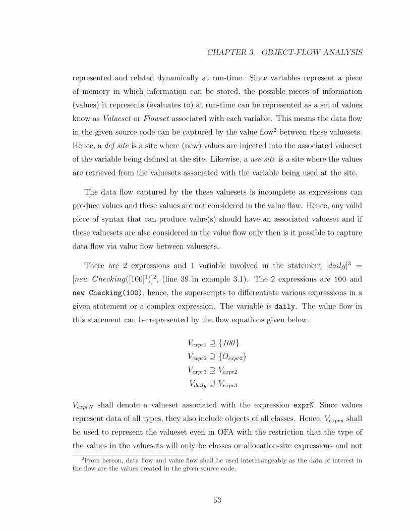
CHAPTER 3. OBJECT-FLOW ANALYSIS
represented and related dynamically at run-time. Since variables represent a piece
of memory in which information can be stored, the possible pieces of information
(values) it represents (evaluates to) at run-time can be represented as a set of values
know as Valueset or Flowset associated with each variable. This means the data flow
in the given source code can be captured by the value flow2 between these valuesets.
Hence, a def site is a site where (new) values are injected into the associated valueset
of the variable being defined at the site. Likewise, a use site is a site where the values
are retrieved from the valuesets associated with the variable being used at the site.
The data flow captured by the these valuesets is incomplete as expressions can
produce values and these values are not considered in the value flow. Hence, any valid
piece of syntax that can produce value(s) should have an associated valueset and if
these valuesets are also considered in the value flow only then is it possible to capture
data flow via value flow between valuesets.
There are 2 expressions and 1 variable involved in the statement [daily]3 =
[new Checking([100]1)]2, (line 39 in example 3.1). The 2 expressions are 100 and
new Checking(100), hence, the superscripts to differentiate various expressions in a
given statement or a complex expression. The variable is daily. The value flow in
this statement can be represented by the flow equations given below.
Vexpr1 ⊇ {100}Vexpr2 ⊇ {Oexpr2}Vexpr3 ⊇ Vexpr2
Vdaily ⊇ Vexpr3
VexprN shall denote a valueset associated with the expression exprN. Since values
represent data of all types, they also include objects of all classes. Hence, Vexprn shall
be used to represent the valueset even in OFA with the restriction that the type of
the values in the valuesets will only be classes or allocation-site expressions and not
2From hereon, data flow and value flow shall be used interchangeably as the data of interest inthe flow are the values created in the given source code.
53
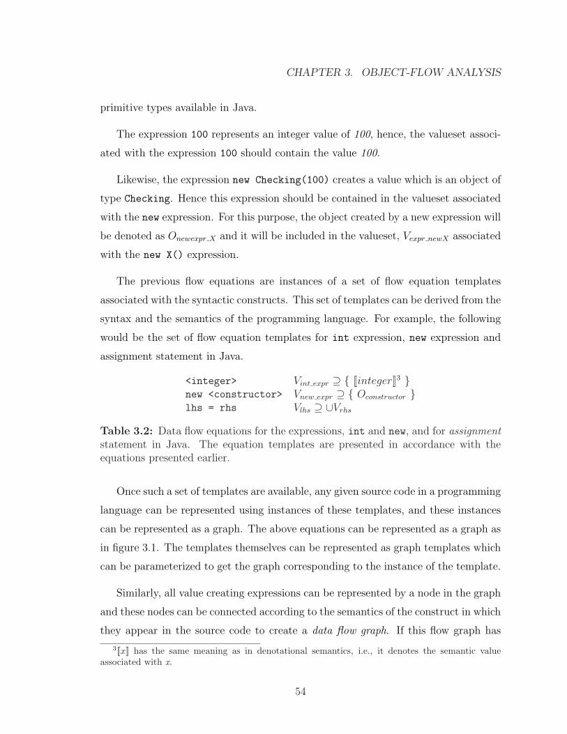
CHAPTER 3. OBJECT-FLOW ANALYSIS
primitive types available in Java.
The expression 100 represents an integer value of 100, hence, the valueset associ-
ated with the expression 100 should contain the value 100.
Likewise, the expression new Checking(100) creates a value which is an object of
type Checking. Hence this expression should be contained in the valueset associated
with the new expression. For this purpose, the object created by a new expression will
be denoted as Onewexpr X and it will be included in the valueset, Vexpr newX associated
with the new X() expression.
The previous flow equations are instances of a set of flow equation templates
associated with the syntactic constructs. This set of templates can be derived from the
syntax and the semantics of the programming language. For example, the following
would be the set of flow equation templates for int expression, new expression and
assignment statement in Java.
<integer> Vint expr ⊇ { [[integer]]3 }new <constructor> Vnew expr ⊇ { Oconstructor }lhs = rhs Vlhs ⊇ ∪Vrhs
Table 3.2: Data flow equations for the expressions, int and new, and for assignmentstatement in Java. The equation templates are presented in accordance with theequations presented earlier.
Once such a set of templates are available, any given source code in a programming
language can be represented using instances of these templates, and these instances
can be represented as a graph. The above equations can be represented as a graph as
in figure 3.1. The templates themselves can be represented as graph templates which
can be parameterized to get the graph corresponding to the instance of the template.
Similarly, all value creating expressions can be represented by a node in the graph
and these nodes can be connected according to the semantics of the construct in which
they appear in the source code to create a data flow graph. If this flow graph has
3[[x]] has the same meaning as in denotational semantics, i.e., it denotes the semantic valueassociated with x.
54
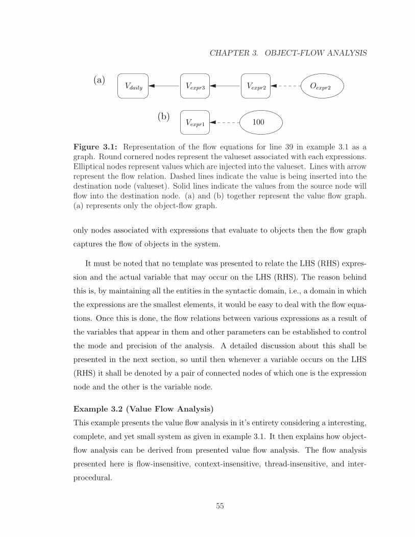
CHAPTER 3. OBJECT-FLOW ANALYSIS
Vdaily Vexpr3 Vexpr2 Oexpr2
100Vexpr1(b)
(a)
Figure 3.1: Representation of the flow equations for line 39 in example 3.1 as agraph. Round cornered nodes represent the valueset associated with each expressions.Elliptical nodes represent values which are injected into the valueset. Lines with arrowrepresent the flow relation. Dashed lines indicate the value is being inserted into thedestination node (valueset). Solid lines indicate the values from the source node willflow into the destination node. (a) and (b) together represent the value flow graph.(a) represents only the object-flow graph.
only nodes associated with expressions that evaluate to objects then the flow graph
captures the flow of objects in the system.
It must be noted that no template was presented to relate the LHS (RHS) expres-
sion and the actual variable that may occur on the LHS (RHS). The reason behind
this is, by maintaining all the entities in the syntactic domain, i.e., a domain in which
the expressions are the smallest elements, it would be easy to deal with the flow equa-
tions. Once this is done, the flow relations between various expressions as a result of
the variables that appear in them and other parameters can be established to control
the mode and precision of the analysis. A detailed discussion about this shall be
presented in the next section, so until then whenever a variable occurs on the LHS
(RHS) it shall be denoted by a pair of connected nodes of which one is the expression
node and the other is the variable node.
Example 3.2 (Value Flow Analysis)
This example presents the value flow analysis in it’s entirety considering a interesting,
complete, and yet small system as given in example 3.1. It then explains how object-
flow analysis can be derived from presented value flow analysis. The flow analysis
presented here is flow-insensitive, context-insensitive, thread-insensitive, and inter-
procedural.
55
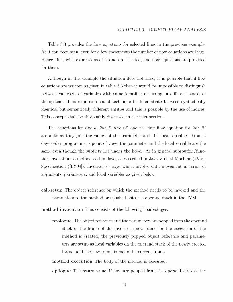
CHAPTER 3. OBJECT-FLOW ANALYSIS
Table 3.3 provides the flow equations for selected lines in the previous example.
As it can been seen, even for a few statements the number of flow equations are large.
Hence, lines with expressions of a kind are selected, and flow equations are provided
for them.
Although in this example the situation does not arise, it is possible that if flow
equations are written as given in table 3.3 then it would be impossible to distinguish
between valuesets of variables with same identifier occurring in different blocks of
the system. This requires a sound technique to differentiate between syntactically
identical but semantically different entities and this is possible by the use of indices.
This concept shall be thoroughly discussed in the next section.
The equations for line 3, line 6, line 26, and the first flow equation for line 21
are alike as they join the values of the parameter and the local variable. From a
day-to-day programmer’s point of view, the parameter and the local variable are the
same even though the subtlety lies under the hood. As in general subroutine/func-
tion invocation, a method call in Java, as described in Java Virtual Machine (JVM)
Specification ([LY99]), involves 5 stages which involve data movement in terms of
arguments, parameters, and local variables as given below.
call-setup The object reference on which the method needs to be invoked and the
parameters to the method are pushed onto the operand stack in the JVM.
method invocation This consists of the following 3 sub-stages.
prologue The object reference and the parameters are popped from the operand
stack of the frame of the invoker, a new frame for the execution of the
method is created, the previously popped object reference and parame-
ters are setup as local variables on the operand stack of the newly created
frame, and the new frame is made the current frame.
method execution The body of the method is executed.
epilogue The return value, if any, are popped from the operand stack of the
56
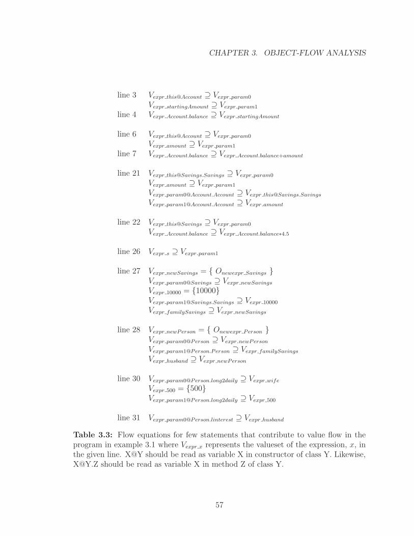
CHAPTER 3. OBJECT-FLOW ANALYSIS
line 3 Vexpr this@Account ⊇ Vexpr param0
Vexpr startingAmount ⊇ Vexpr param1
line 4 Vexpr Account.balance ⊇ Vexpr startingAmount
line 6 Vexpr this@Account ⊇ Vexpr param0
Vexpr amount ⊇ Vexpr param1
line 7 Vexpr Account.balance ⊇ Vexpr Account.balance+amount
line 21 Vexpr [email protected] ⊇ Vexpr param0
Vexpr amount ⊇ Vexpr param1
Vexpr [email protected] ⊇ Vexpr [email protected]
Vexpr [email protected] ⊇ Vexpr amount
line 22 Vexpr this@Savings ⊇ Vexpr param0
Vexpr Account.balance ⊇ Vexpr Account.balance∗4.5
line 26 Vexpr s ⊇ Vexpr param1
line 27 Vexpr newSavings = { Onewexpr Savings }Vexpr param0@Savings ⊇ Vexpr newSavings
Vexpr 10000 = {10000}Vexpr [email protected] ⊇ Vexpr 10000
Vexpr familySavings ⊇ Vexpr newSavings
line 28 Vexpr newPerson = { Onewexpr Person }Vexpr param0@Person ⊇ Vexpr newPerson
Vexpr [email protected] ⊇ Vexpr familySavings
Vexpr husband ⊇ Vexpr newPerson
line 30 Vexpr [email protected] ⊇ Vexpr wife
Vexpr 500 = {500}Vexpr [email protected] ⊇ Vexpr 500
line 31 Vexpr [email protected] ⊇ Vexpr husband
Table 3.3: Flow equations for few statements that contribute to value flow in theprogram in example 3.1 where Vexpr x represents the valueset of the expression, x, inthe given line. X@Y should be read as variable X in constructor of class Y. Likewise,[email protected] should be read as variable X in method Z of class Y.
57
CHAPTER 3. OBJECT-FLOW ANALYSIS
current frame, pushed onto the operand stack of the frame of the invoker,
and invoker’s frame is made the current frame.
call-return The return value, if any, is popped from the operand stack of the current
frame and “assigned” to the assignee.
End of Example
The above description deals with the details of how method invocation occurs in
the JVM whereas the discussion till now has been in the realms of Java language.
Hence, there are two options in which to model the data flow. The first option is
to model the data flow as it occurs in the source code, i.e., as represented in Java
language. The second being to model the data flow as it occurs in the JVM via
the execution of the bytecodes compiled from the source code. The second option is
favored as the source code for all the components of the system being analyzed may
not be available. However, the bytecodes for all the non-native code being used in
the system will be available, and if a convenient representation can be constructed
from these bytecodes then any system written in Java can be analyzed provided it’s
class files are available. This issue is further discussed in the next chapter.
Equations for line 4 and line 7 and the first equation for line 21 are simple as-
signment statements involving integer valued expressions. By the semantics of the
assignment statement in Java, at run-time the assignee takes on the values the rhs
expression evaluates to, and this is represented by the flow equations. Although the
lhs expressions are member variables, the way in which local variables would be dealt
would be no different.
In short, the way in which assignments are dealt will be same no matter what is
the type of the lhs and/or rhs expressions while the notable difference will be in the
evaluation of the expressions and the way in which the valuesets of expressions are
related to valuesets of the identifiers.
Equations for line 22 and line 26 correspond to the new expression and the assign-
ment of the new object to the identifier on the lhs. By the semantics of Java as given
58
CHAPTER 3. OBJECT-FLOW ANALYSIS
in [LY99], a new expression is translated into more than one instruction in terms of
bytecode. The first being an instruction to create a new object. This instruction just
allocates memory space for the object. This is followed by a call to the constructor of
the class of the object via the invokespecial bytecode. Since the call is on an object
the arguments to the invocation needs to be setup suitably. The newly created object
will be the this or the zeroth (param0) parameter. The arguments are suitably setup
as described earlier. Once the call returns after the execution of the constructor the
top of the operand stack is popped as the result of the newly created and initialized
object. Now the equations shall be mapped to the actions described here. The first
equation represents the action of allocating memory to the new object. The second
and the third represent the setting up of arguments to call the constructor. The last
equation represent the assignment of the reference of the newly created and initialized
object to lhs. There is no equations to setup the arguments in the method call as it
is accomplished when entering the method body.
The only distinction between the two lines of code considered here is the type
of the parameter to the constructor. It is interesting to notice that the set of value
flow equations instantiated is not affected by the type of parameters or variables but
rather by the expressions being considered for the analysis. This is true if the program
being considered is type correct.
Equations two through four for line 21 correspond to the call super(amount) in
class Savings. A call to super is a call to the constructor of the super class, hence,
it is treated as explained in the previous paragraph.
Equations for line 30 and line 31 correspond to the method invocation. The
real distinction would be the calls that occur in the body of these method calls.
The call in line 30 will result in two calls to methods defined in Account and not
overridden in it’s children classes via a reference variable of type Account. On the
other hand the call in line 31 will result in a call to a method declared in Account
and defined in it’s children classes via a reference variable of type Account. Both
the cases are represented as virtual method invocation in the JVM, and are achieved
59
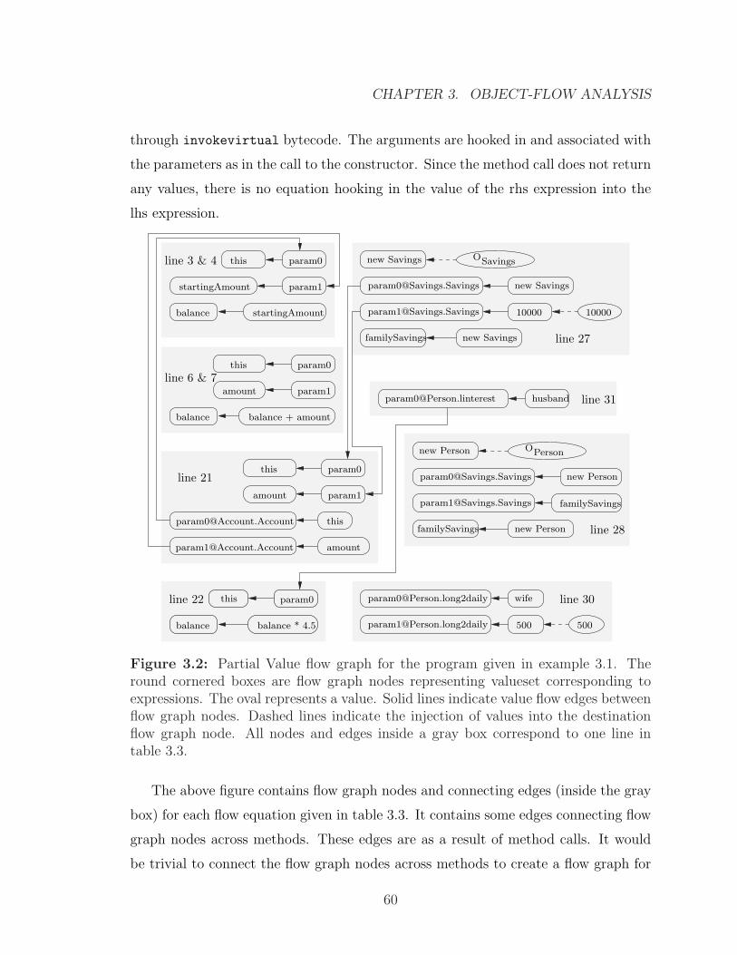
CHAPTER 3. OBJECT-FLOW ANALYSIS
through invokevirtual bytecode. The arguments are hooked in and associated with
the parameters as in the call to the constructor. Since the method call does not return
any values, there is no equation hooking in the value of the rhs expression into the
lhs expression.
balance balance * 4.5
param0thisline 22
balance balance + amount
amount param1
param0this
line 6 & 7
param0
startingAmount param1
balance startingAmount
thisline 3 & 4
[email protected] this
[email protected] amount
amount param1
param0thisline 21
wife
500 500
[email protected] line 30
new Savings OSavings
new Savings
10000 10000
familySavings new Savings line 27
[email protected] line 31
new Person
new Person
familySavings new Person
OPerson
familySavings
line 28
Figure 3.2: Partial Value flow graph for the program given in example 3.1. Theround cornered boxes are flow graph nodes representing valueset corresponding toexpressions. The oval represents a value. Solid lines indicate value flow edges betweenflow graph nodes. Dashed lines indicate the injection of values into the destinationflow graph node. All nodes and edges inside a gray box correspond to one line intable 3.3.
The above figure contains flow graph nodes and connecting edges (inside the gray
box) for each flow equation given in table 3.3. It contains some edges connecting flow
graph nodes across methods. These edges are as a result of method calls. It would
be trivial to connect the flow graph nodes across methods to create a flow graph for
60
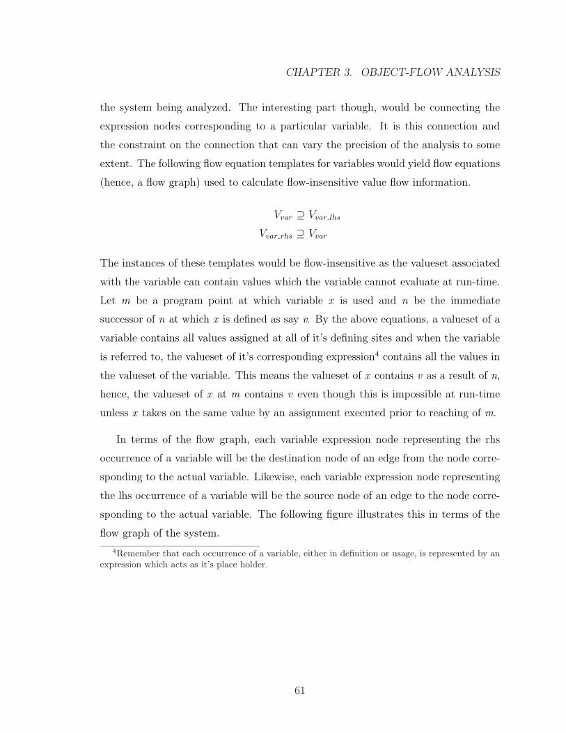
CHAPTER 3. OBJECT-FLOW ANALYSIS
the system being analyzed. The interesting part though, would be connecting the
expression nodes corresponding to a particular variable. It is this connection and
the constraint on the connection that can vary the precision of the analysis to some
extent. The following flow equation templates for variables would yield flow equations
(hence, a flow graph) used to calculate flow-insensitive value flow information.
Vvar ⊇ Vvar lhs
Vvar rhs ⊇ Vvar
The instances of these templates would be flow-insensitive as the valueset associated
with the variable can contain values which the variable cannot evaluate at run-time.
Let m be a program point at which variable x is used and n be the immediate
successor of n at which x is defined as say v. By the above equations, a valueset of a
variable contains all values assigned at all of it’s defining sites and when the variable
is referred to, the valueset of it’s corresponding expression4 contains all the values in
the valueset of the variable. This means the valueset of x contains v as a result of n,
hence, the valueset of x at m contains v even though this is impossible at run-time
unless x takes on the same value by an assignment executed prior to reaching of m.
In terms of the flow graph, each variable expression node representing the rhs
occurrence of a variable will be the destination node of an edge from the node corre-
sponding to the actual variable. Likewise, each variable expression node representing
the lhs occurrence of a variable will be the source node of an edge to the node corre-
sponding to the actual variable. The following figure illustrates this in terms of the
flow graph of the system.
4Remember that each occurrence of a variable, either in definition or usage, is represented by anexpression which acts as it’s place holder.
61
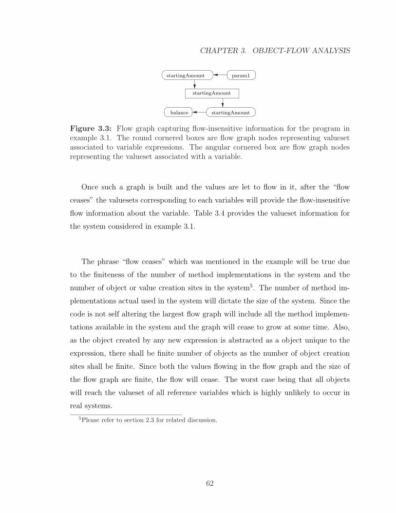
CHAPTER 3. OBJECT-FLOW ANALYSIS
startingAmount param1
balance startingAmount
startingAmount
Figure 3.3: Flow graph capturing flow-insensitive information for the program inexample 3.1. The round cornered boxes are flow graph nodes representing valuesetassociated to variable expressions. The angular cornered box are flow graph nodesrepresenting the valueset associated with a variable.
Once such a graph is built and the values are let to flow in it, after the “flow
ceases” the valuesets corresponding to each variables will provide the flow-insensitive
flow information about the variable. Table 3.4 provides the valueset information for
the system considered in example 3.1.
The phrase “flow ceases” which was mentioned in the example will be true due
to the finiteness of the number of method implementations in the system and the
number of object or value creation sites in the system5. The number of method im-
plementations actual used in the system will dictate the size of the system. Since the
code is not self altering the largest flow graph will include all the method implemen-
tations available in the system and the graph will cease to grow at some time. Also,
as the object created by any new expression is abstracted as a object unique to the
expression, there shall be finite number of objects as the number of object creation
sites shall be finite. Since both the values flowing in the flow graph and the size of
the flow graph are finite, the flow will cease. The worst case being that all objects
will reach the valueset of all reference variables which is highly unlikely to occur in
real systems.
5Please refer to section 2.3 for related discussion.
62
CHAPTER 3. OBJECT-FLOW ANALYSIS
Reference Variables ValuesetfamilySavings:Account(Family.main) { [new Savings(10000)]@line 27 }husband:Person(Family.main) { [new Person(familySavings)]@line 28 }wife:Person(Family.main) { [new Person(familySavings)]@line 29 }longterm:Account(Person) { [new Savings(10000)]@line 27 }daily:Account(Person) { [new Checking(100)]@line 39 }this:Person(Person.Person) { [new Person(familySavings)]@line 28,
[new Person(familySavings)]@line 29 }yourLongTerm:Account(Person.Person) { [new Savings(10000)]@line 27 }this:Person(Person.long2daily) { [new Person(familySavings)]@line 29 }amount:int(Person.long2daily) { [500]@line 28 }this:Person(Person.linterest) { [new Person(familySavings)]@line 28 }this:Checking(Checking.Checking) { [new Checking(100)]@line 39 }amount:int(Checking.Checking) { [100]@line 39 }this:Checking(Checking.interest) { [new Checking(100)]@line 39 }this:Savings(Savings.Savings) { [new Savings(10000)]@line 27 }amount:int(Savings.Savings) { [10000]@line 27 }this:Savings(Savings.interest) { [new Savings(10000)]@line 27 }balance:int(Account) { [10000]@line 27, [100]@line 39,
[balance + amount]@line 10,[balance - amount]@line 7,[balance * 4.5]@line 22 }
this:Account(Account.Account) { [new Savings(10000)]@line 27 }[new Checking(100)]@line 39
startingAmount:int(Account.Account) { [10000]@line 27, [100]@line 39 }this:Account(Account.deposit) { [new Checking(100)]@line 39 }amount:int(Account.deposit) { [500]@line 28 }this:Account(Account.withdraw) { [new Savings(10000)]@line 27 }amount:int(Account.withdraw) { [500]@line 28 }
Table 3.4: Summary of value flow in the program given in example 3.1. X:Y(Z) isto be read as variable X of type Y declared in Z. The unshaded rows together formthe object flow information.
63
CHAPTER 3. OBJECT-FLOW ANALYSIS
3.3 In Theory
The previous section gave a thorough but still a birds-eye view of value flow analysis.
There were questions related to the relation/connection between expression nodes and
variable nodes and ways by which the precision of the analysis can be varied. These
questions shall be answered in this section after discussing the common approaches
to specify such analyses.
3.3.1 Common Approaches
As presented in [NNH99]6 there are more than one approach to program analysis,
and among them Data Flow Analysis and Constraint Based Analysis are of relevance
in this document.
Data Flow Analysis
Data flow analysis7, is an approach in which the given program will be traversed
till the information being collected reaches a fixed point. When a program point is
traversed, the incoming data-flow information (carrier) is transformed by applying
a transfer function to yield the data-flow information to be used when traversing
the successive program point. This form of analysis is defined by providing a pair
of functions for each possible construct in the source language. Typically, these are
gen and kill function. As the name suggests, gen function adds or generates new
information while kill function removes or kills information. The transfer function
for an analysis is usually defined in terms of these functions. The solution to the
analysis occurs when the equations containing gen and kill functions and relating
information set with equality are satisfied.
6It is one source which discusses in detail the four most common approaches to specify programanalysis.
7Note that Data flow analysis presented here is an approach to perform program analysis andthe one discussed previously is an analysis that calculates the data flow information.
64
CHAPTER 3. OBJECT-FLOW ANALYSIS
We are trying to be general when we use phrases like “the program will be tra-
versed” and “the successive program point”. This is deliberate as the traversing
might start from the last program point and move towards the first program point.
Hence, analysis has a direction associated with it. If the analysis starts from the first
program point of the program and proceeds towards the last program point then it
is called as forward analysis. It’s counterpart in which the analysis starts from the
last program point and proceeds towards the first program point is called as backward
analysis.
It is possible that an analysis will calculate information which is (must be) true.
Likewise it possible that an analysis will calculate information which may be true.
Hence, DFA can be categorized depending on whether the analysis produces must or
may information.
There are two approaches in DFA. The one described above is the equational
approach to DFA. On the other hand if inclusion (constraints) is used to relate sets
of information then it is known as constraint based approach to DFA. It should be
noted that equations can be easily obtained from constraints and vice versa. The
equational approach is more restricted compared to constraint based approach as it
uses equality while the latter uses subset to relate the information set(s).
Constraint-based Analysis
Constraint based analysis is similar to the constraint based approach to data flow
analysis. This uses inclusions to relate to set of information. The distinction ends
there. In this approach, an information set is associated with each program point
in the program and each variable in the program. An analysis is defined by provid-
ing constraint template for each possible syntactic construct in the source language.
These constraint templates will relate the previously mentioned information sets. The
analysis usually proceeds in two phases. The first phase involves the instantiation of
the templates corresponding to chunks of the give program. This phase will initialize
65
CHAPTER 3. OBJECT-FLOW ANALYSIS
few of the information sets. The following phase will solve these constraint instances
to obtain the solution to the analysis. It is possible for new constraint instances to be
created in the second phase when handling functional and object-oriented languages.
In classical literature, ρ function maps a variable in the program to it’s information
set. Likewise, C function maps a program point in the program to it’s information
set. By now, it should be clear that an analysis instrumented as data flow analysis
can be trivially realized as a constraint based analysis.
As the ρ and C provide a layer of abstraction, by changing the function suitably
it is trivial to obtain different flavours, i.e., context-sensitive or flow-sensitive.
It should be noted that, traditionally constraint based analysis is associated with
control flow analysis. However, it is possible to implement analyses implemented in
data flow analysis style, as constraint based analysis. Hence, constraint based analysis
is as good an approach as data flow analysis to implement program analysis.
3.3.2 Varying Precision in Constraint-based Analysis
Given the basics of constraint based analysis, how various modes of precision can be
achieved in constraint based analysis will give sufficient grounds before presenting
object-flow analysis as a constraint based analysis. In the following discussion, we
shall use terms such as variables and values to make the discussion general, but we
will use specific terms such as reference variables and objects when required.
Flow-insensitive
When an analysis operates in flow-insensitive mode, all occurrence of a variable (not
the identifier) are indistinguishable, i.e., there is only one summary set8 associated
with the variable independent of the location of the variable in the program. Now
considering ρ, the function will accept a variable and the enclosing method (if any)
8From hereon, summary set shall be used as a synonym for information set.
66
CHAPTER 3. OBJECT-FLOW ANALYSIS
and return a summary set associated with the variable. When a value is assigned to
the variable, the summary set associated with the variable needs to be altered. This
is done by assigning a new image to the variable in ρ. C function would accept a
label and return the summary set associated with the expression in that label.
Relating this back to example 3.1, the Valuesets associated with the variables will
be the summary sets as returned by ρ and Valuesets associated with the AST nodes
associated with expressions will be the summary sets as returned by C.
Flow-sensitive
In this mode each occurrence of a variable is distinguishable, i.e., each occurrence of
variable is associated with a unique summary set. Now considering ρ, the function
will now map a single variable to many summary sets which can be distinguished
on the basis of the label. This means that ρ will accept a variable, the enclosing
method (if any), and a label, and it will return the summary set associated with the
occurrence of the variable at the given label. C is identical to that in flow-insensitive
mode as it maps a label to a summary set which is the requisite for flow-sensitive
mode. An interesting observation is that C essential encompasses all the information
in ρ if each expression in the program is considered as a program point.
Context-sensitive
The two modes discussed previously are context-insensitive. In other words, the
information or summary set associated with a variable or label is independent of any
context such as calling sequence or the related object. Let’s consider calling sequence
as a context. There can be an (in)finitely long calling sequence possible in a given
program. For a feasible and tractable analysis, we need to restrict the length of the
calling sequence considered during the analysis. Assume that the length is a constant
k. This means any context of length k or less will be considered to distinguish the
summary sets associated with a variable. In terms of ρ, the function will accept a
67
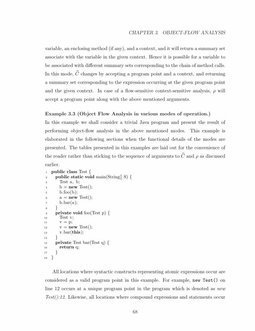
CHAPTER 3. OBJECT-FLOW ANALYSIS
variable, an enclosing method (if any), and a context, and it will return a summary set
associate with the variable in the given context. Hence it is possible for a variable to
be associated with different summary sets corresponding to the chain of method calls.
In this mode, C changes by accepting a program point and a context, and returning
a summary set corresponding to the expression occurring at the given program point
and the given context. In case of a flow-sensitive context-sensitive analysis, ρ will
accept a program point along with the above mentioned arguments.
Example 3.3 (Object Flow Analysis in various modes of operation.)
In this example we shall consider a trivial Java program and present the result of
performing object-flow analysis in the above mentioned modes. This example is
elaborated in the following sections when the functional details of the modes are
presented. The tables presented in this examples are laid out for the convenience of
the reader rather than sticking to the sequence of arguments to C and ρ as discussed
earlier.
1 public class Test {2 public static void main(String[] S) {3 Test a, b;4 b = new Test();5 b.foo(b);6 a = new Test();7 b.bar(a);8 }9 private void foo(Test p) {
10 Test v;11 v = p;12 v = new Test();13 v.bar(this);14 }15 private Test bar(Test q) {16 return q;17 }18 }
All locations where syntactic constructs representing atomic expressions occur are
considered as a valid program point in this example. For example, new Test() on
line 12 occurs at a unique program point in the program which is denoted as new
Test():12. Likewise, all locations where compound expressions and statements occur
68
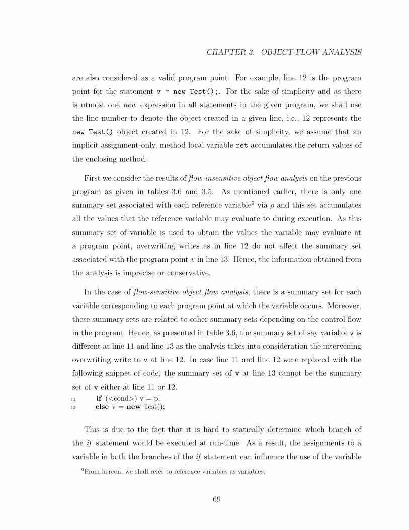
CHAPTER 3. OBJECT-FLOW ANALYSIS
are also considered as a valid program point. For example, line 12 is the program
point for the statement v = new Test();. For the sake of simplicity and as there
is utmost one new expression in all statements in the given program, we shall use
the line number to denote the object created in a given line, i.e., 12 represents the
new Test() object created in 12. For the sake of simplicity, we assume that an
implicit assignment-only, method local variable ret accumulates the return values of
the enclosing method.
First we consider the results of flow-insensitive object flow analysis on the previous
program as given in tables 3.6 and 3.5. As mentioned earlier, there is only one
summary set associated with each reference variable9 via ρ and this set accumulates
all the values that the reference variable may evaluate to during execution. As this
summary set of variable is used to obtain the values the variable may evaluate at
a program point, overwriting writes as in line 12 do not affect the summary set
associated with the program point v in line 13. Hence, the information obtained from
the analysis is imprecise or conservative.
In the case of flow-sensitive object flow analysis, there is a summary set for each
variable corresponding to each program point at which the variable occurs. Moreover,
these summary sets are related to other summary sets depending on the control flow
in the program. Hence, as presented in table 3.6, the summary set of say variable v is
different at line 11 and line 13 as the analysis takes into consideration the intervening
overwriting write to v at line 12. In case line 11 and line 12 were replaced with the
following snippet of code, the summary set of v at line 13 cannot be the summary
set of v either at line 11 or 12.
11 if (<cond>) v = p;12 else v = new Test();
This is due to the fact that it is hard to statically determine which branch of
the if statement would be executed at run-time. As a result, the assignments to a
variable in both the branches of the if statement can influence the use of the variable
9From hereon, we shall refer to reference variables as variables.
69
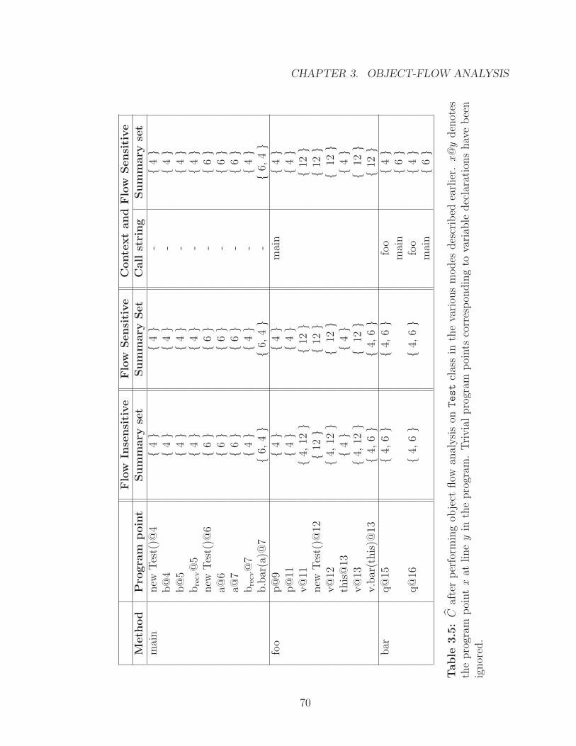
CHAPTER 3. OBJECT-FLOW ANALYSIS
Flo
wIn
sensi
tive
Flo
wSensi
tive
Conte
xt
and
Flo
wSensi
tive
Meth
od
Pro
gra
mpoin
tSum
mary
set
Sum
mary
Set
Call
stri
ng
Sum
mary
set
mai
nnew
Tes
t()@
4{4}
{4}
-{4}
b@
4{4}
{4}
-{4}
b@
5{4}
{4}
-{4}
bre
cv@
5{4}
{4}
-{4}
new
Tes
t()@
6{6}
{6}
-{6}
a@6
{6}
{6}
-{6}
a@7
{6}
{6}
-{6}
bre
cv@
7{4}
{4}
-{4}
b.b
ar(a
)@7
{6,4}
{6,4}
-{6
,4}
foo
p@
9{4}
{4}
mai
n{4}
p@
11{4}
{4}
{4}
v@
11{4
,12}
{12}
{12}
new
Tes
t()@
12{1
2}
{12}
{12}
v@
12{4
,12}
{12}
{12}
this
@13
{4}
{4}
{4}
v@
13{4
,12}
{12}
{12}
v.b
ar(t
his
)@13
{4,6}
{4,6}
{12}
bar
q@
15{4
,6}
{4,6}
foo
{4}
mai
n{6}
q@
16{4
,6}
{4,6}
foo
{4}
mai
n{6}
Table
3.5
:C
afte
rper
form
ing
obje
ctflow
anal
ysi
son
Test
clas
sin
the
vari
ous
modes
des
crib
edea
rlie
r.x@
yden
otes
the
pro
gram
poi
nt
xat
line
yin
the
pro
gram
.Tri
via
lpro
gram
poi
nts
corr
espon
din
gto
vari
able
dec
lara
tion
shav
ebee
nig
nor
ed.
70
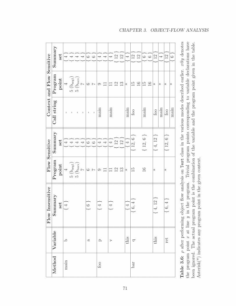
CHAPTER 3. OBJECT-FLOW ANALYSIS
Flo
wIn
sensi
tive
Flo
wSensi
tive
Conte
xt
and
Flo
wSensi
tive
Meth
od
Vari
able
Sum
mary
Pro
gra
mSum
mary
Call
stri
ng
Pro
gra
mSum
mary
set
poin
tse
tpoin
tse
tm
ain
b{4}
4{4}
-4
{4}
5(b
arg
1)
{4}
-5
(barg
1)
{4}
5(b
recv
){4}
-5
(bre
cv)
{4}
7{4}
-7
{4}
a{6}
6{6}
-6
{6}
7{6}
-7
{6}
foo
p{4}
9{4}
mai
n9
{4}
11{4}
11{4}
v{4}
11{4}
mai
n11
{4}
12{1
2}
12{1
2}
13{1
2}
13{1
2}
this
{4}
*{4}
mai
n*
{4}
bar
q{6
,4}
15{1
2,6}
foo
15{1
2}
16{1
2}
16{1
2,6}
mai
n15
{6}
16{6}
this
{4,12}
*{4
,12}
foo
*{1
2}
mai
n*
{4}
ret
{6,4}
*{1
2,6}
foo
*{1
2}
mai
n*
{6}
Table
3.6
:ρ
afte
rper
form
ing
obje
ctflow
anal
ysi
son
Test
clas
sin
the
vari
ous
modes
des
crib
edea
rlie
r.x@
yden
otes
the
pro
gram
poi
nt
xat
line
yin
the
pro
gram
.Tri
via
lpro
gram
poi
nts
corr
espon
din
gto
vari
able
dec
lara
tion
shav
ebee
nig
nor
ed.
The
actu
alpro
gram
poi
nt
isth
eco
mbin
atio
nof
the
vari
able
and
the
pro
gram
poi
nt
give
nin
the
table
.A
ster
isk(*
)in
dic
ates
any
pro
gram
poi
nt
inth
egi
ven
conte
xt.
71
CHAPTER 3. OBJECT-FLOW ANALYSIS
in following statements. Hence, the summary set of v at line 13 would be the result
of merging of the summary sets of v at line 11 and 12. In case of object flow analysis,
union operation on sets would be merging operation.
An asterisk(*) is associated with this variable in case of methods foo and bar to
indicate that values associated with this variable does not change with the program
point inside a given method. This is due to the fact that this is a final local variable
in a given instance method. Although ret can accumulate return values at different
program points, it’s purpose and concept makes it program point independent. Hence,
asterisk(*) is used as the program point in the program point columns of table 3.6.
In flow-sensitive mode of OFA, some of the values that could not have reached a
program point during the execution of the program have been weeded out, but not
all. The information from the analysis indicates that the Test object created at line
12 can be returned to the call-site of bar at line 7. A similar issue at the call-site of
bar at line 13. This is incorrect, and it stems from the fact that the summary sets
associated with the program points and the locals in a method are independent of
the caller of the method, i.e., the context of execution does not bear any impact on
the summary set.
The above mentioned problem can be solved by performing context-sensitive object
flow analysis where call string is the context. Call string of maximum length 1 is
considered as the context in tables 3.5 and 3.6. This means that the number of
summary sets maintained for a single variable or program point in a method is equal
to the number of unique callers of the method. In terms of C and ρ, as discussed
earlier, each now have a new column(parameter) in the given tables for the context
information named as call string. This parameter splits the information associated
with a program point or a variable into more precise sets as it is evident from the
tables for entities in method bar.
End of Example
72
CHAPTER 3. OBJECT-FLOW ANALYSIS
The previous example only handled local variables deserting static variables and
instance variables. Static variables can be considered as global variables when com-
bined with the enclosing class name. Hence, in terms of information calculation, it
is similar to calculation of information of unique local variables with the exception
that suitable assumptions about the control flow needs to be made when considering
method boundaries in context-sensitive mode.
Instance variables can also be handled like static variables, but it would provide
overly approximate results. On the other hand, handling instance variables based on
object creation sites can improve precision although it will be approximate in the sense
that the fields of objects created at an object creation site cannot be differentiated,
i.e., the fields of objects created by an object creation site in a loop. However, in such
cases a static analysis which can determine if two use sites will use the same object
via control flow can improve the precision of information pertaining to fields.
Given the results of OFA on a program, the next section provides the details on
how can this be achieved algorithmically. Before we proceed, we round up by high-
lighting certain points evident from the tables presented in the previous example.
The amount of meta-information, i.e., the information maintained about the infor-
mation, increases as the demand on the precision of the information escalates. In the
case of flow-insensitive and flow-sensitive modes of the analysis the increase in pre-
cision of the information is more compared to the increase in the meta-information.
However, in case of context-sensitive and simple flow-sensitive modes of the analysis,
the increase in meta-information is comparable to the increase in the precision of the
information. These observations prompt the developers to justify the cost involved in
increasing the precision of the information. It is also evident from the tables that the
meta-information increases in exponential order, i.e., the number of choices to reach
the information set increases, as the precision improves.
73
CHAPTER 3. OBJECT-FLOW ANALYSIS
3.4 Constraints for Object-Flow Analysis
In this section we shall present constraint templates required to perform object-flow
analysis on a given Java program. We shall present the constraint system to perform
the analysis in the most simple and imprecise mode, i.e., flow-insensitive mode. The
constraint systems to perform analysis in flow-sensitive mode and context-sensitive
mode are presented as a specialization of the constraint system presented for flow-
insensitive mode.
Before we proceed to the constraint system used to define the analysis, the question
“How are arrays handled?” needs to be answered. We propose to handle arrays by
considering each array type as a class10 by itself. For example, given an expression
int[x][y][z], there exists 3 classes each corresponding to int[][][], int[][], and
int[]. Each array type or class is associated with a summary set and this leads to
overly pessimistic results. It would be trivial to associate a summary set with the
combination of array type and array object creation site and this will improve the
precision of the analysis.
3.4.1 Flow-insensitive Mode
We present the constraint system to achieve object-flow analysis in flow-insensitive
mode in this section.
Following are the domains over which the functions in the constraint system op-
erate.
A Set of array types (classes) of non-primitive base types. A ⊆ C.
B Set containing boolean values, true and false.
C Set of Java classes in the given software.
10In terms of Java literature, each array type is a class by itself. Please refer to section 2.15 of[LY99] and/or chapter 10 of [GJS00] for further details.
74
CHAPTER 3. OBJECT-FLOW ANALYSIS
M Set of method definitions in the given software.
IN Set of natural numbers.
P Set of program points in the given software. The elements in this set are further
split into the following sets.
Paa Set of program points corresponding to array access expressions involving
array variables.
Pi Set of program points corresponding to method invocation expressions. pi
represents an element in this set. Pi ⊆ Pr.
Pl Set of program points corresponding to l-value expressions. pl represents
an element in this set.
Po Set of program points corresponding to object creating expressions. An
object creating program point abstracts all the objects created at that
particular program point. Po ⊆ Pr.
PnewT Set of program points corresponding to non-array object creating
expressions. pnewT represents an element in this set.
PnewT [] Set of program points corresponding to array object creating ex-
pressions. pnewT [] represents an element in this set. PnewT [] = Po\PnewT .
Pr Set of program points corresponding to r-value expressions. This also
include expressions which evaluate to void. pr represents an element in
this set. Pr = P\Pl.
Pv Set of program points corresponding to expressions involving reference vari-
ables. This does not include array access expressions. Pv = P\Paa.
V Set of reference variables in the given software. For convenience, we define
Va ⊆ V as a set of reference variables of array type.
There is no separate domain for fields as a fully qualified name for fields will suffice
to differentiate fields with identical names in different classes. This also means that
75
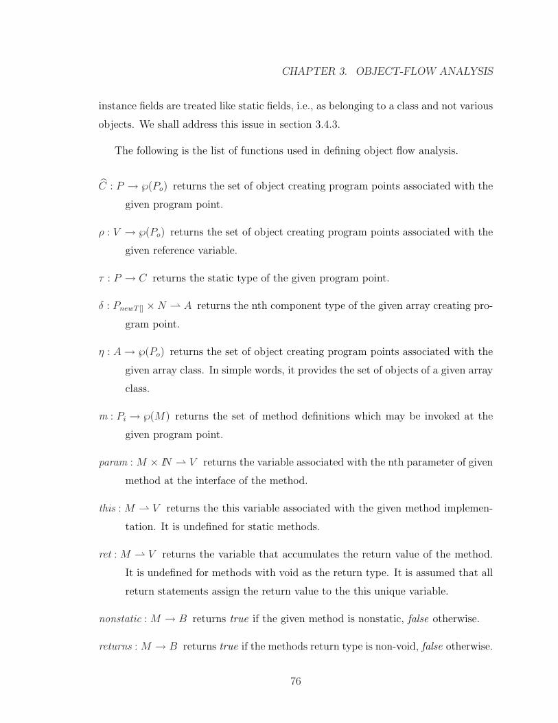
CHAPTER 3. OBJECT-FLOW ANALYSIS
instance fields are treated like static fields, i.e., as belonging to a class and not various
objects. We shall address this issue in section 3.4.3.
The following is the list of functions used in defining object flow analysis.
C : P → ℘(Po) returns the set of object creating program points associated with the
given program point.
ρ : V → ℘(Po) returns the set of object creating program points associated with the
given reference variable.
τ : P → C returns the static type of the given program point.
δ : PnewT [] ×N ⇀ A returns the nth component type of the given array creating pro-
gram point.
η : A→ ℘(Po) returns the set of object creating program points associated with the
given array class. In simple words, it provides the set of objects of a given array
class.
m : Pi → ℘(M) returns the set of method definitions which may be invoked at the
given program point.
param : M × IN ⇀ V returns the variable associated with the nth parameter of given
method at the interface of the method.
this : M ⇀ V returns the this variable associated with the given method implemen-
tation. It is undefined for static methods.
ret : M ⇀ V returns the variable that accumulates the return value of the method.
It is undefined for methods with void as the return type. It is assumed that all
return statements assign the return value to the this unique variable.
nonstatic : M → B returns true if the given method is nonstatic, false otherwise.
returns : M → B returns true if the methods return type is non-void, false otherwise.
76
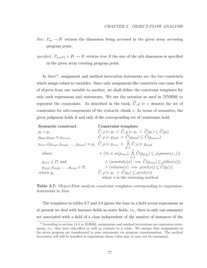
CHAPTER 3. OBJECT-FLOW ANALYSIS
dim : Paa → IN returns the dimension being accessed in the given array accessing
program point.
specified : PnewT [] × IN → B returns true if the size of the nth dimension is specified
in the given array creating program point.
In Java11, assignment and method invocation statements are the two constructs
which assign values to variables. Since only assignment-like constructs can cause flow
of objects from one variable to another, we shall define the constraint templates for
only such expressions and statements. We use the notation as used in [NNH99] to
represent the constraints. As described in the book, C, ρ |= e denotes the set of
constraints for sub-components of the syntactic chunk e. In terms of semantics, the
given judgment holds if and only if the corresponding set of constraints hold.
Syntactic construct Constraint template
pl = pr C, ρ |= pl ∧ C, ρ |= pr ∧ C(pr) ⊆ C(pl)
pbase.pfield ≡ paccess C, ρ |= pfield ∧ C(pfield) ⊆ C(paccess)
precv.i(parg1, parg2, . . . , pargn) ≡ pi C, ρ |= precv ∧n∧
k=1
C, ρ |= pargk
where ∧ (∀x ∈ m(precv).n∧
j=1
C(pargj) ⊆ ρ(param(x , j ))
precv ∈ Pr and ∧ (nonstatic(x) =⇒ C(precv) ⊆ ρ(this(x )))
parg1, parg2, . . . , pargn ∈ Pr ∧ (returns(x) =⇒ ρ(ret(x)) ⊆ C(pi)))
return pr C, ρ |= pr ∧ C(pr) ⊆ ρ(ret(x ))where x is the returning method.
Table 3.7: Object-Flow analysis constraint templates corresponding to expression-statements in Java.
The templates in tables 3.7 and 3.8 ignore the base in a field access expressions as
at present we deal with instance fields as static fields, i.e., there is only one summary
set associated with a field of a class independent of the number of instances of the
11According to section 14.8 in [GJS00], assignments and method invocations are expression state-ments, i.e., they have side-effect as well as evaluate to a value. We assume that assignments inthe given program are transformed to pure statements via program transformation. The methodinvocation will still be handled as expressions whose value may or may not be consumed.
77
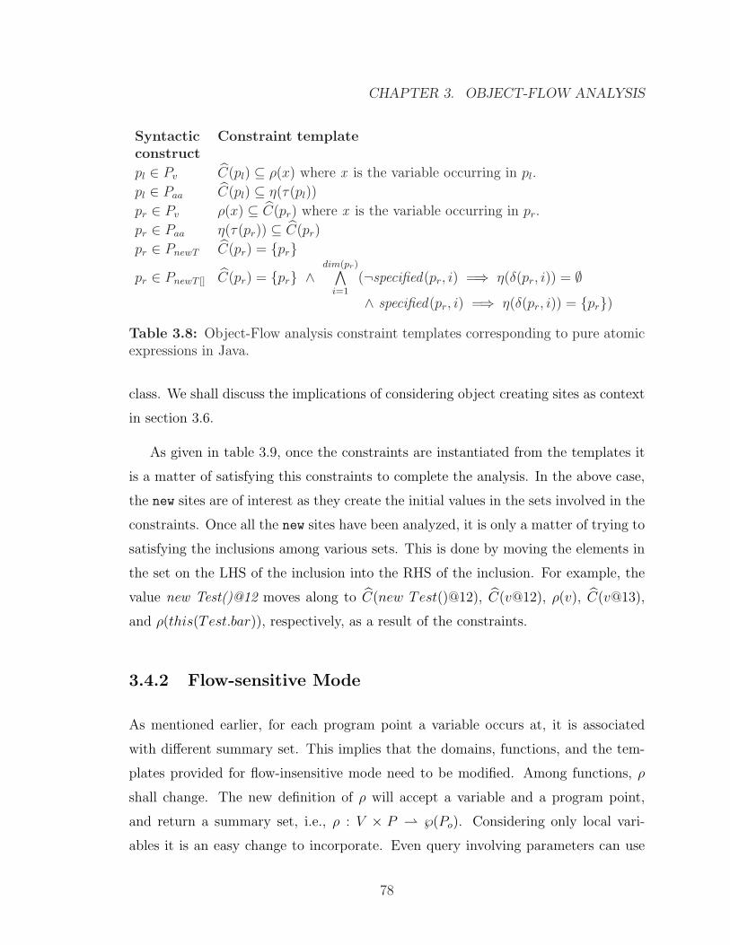
CHAPTER 3. OBJECT-FLOW ANALYSIS
Syntactic Constraint templateconstruct
pl ∈ Pv C(pl) ⊆ ρ(x) where x is the variable occurring in pl.
pl ∈ Paa C(pl) ⊆ η(τ(pl))
pr ∈ Pv ρ(x) ⊆ C(pr) where x is the variable occurring in pr.
pr ∈ Paa η(τ(pr)) ⊆ C(pr)
pr ∈ PnewT C(pr) = {pr}pr ∈ PnewT [] C(pr) = {pr} ∧
dim(pr)∧i=1
(¬specified(pr, i) =⇒ η(δ(pr, i)) = ∅∧ specified(pr, i) =⇒ η(δ(pr, i)) = {pr})
Table 3.8: Object-Flow analysis constraint templates corresponding to pure atomicexpressions in Java.
class. We shall discuss the implications of considering object creating sites as context
in section 3.6.
As given in table 3.9, once the constraints are instantiated from the templates it
is a matter of satisfying this constraints to complete the analysis. In the above case,
the new sites are of interest as they create the initial values in the sets involved in the
constraints. Once all the new sites have been analyzed, it is only a matter of trying to
satisfying the inclusions among various sets. This is done by moving the elements in
the set on the LHS of the inclusion into the RHS of the inclusion. For example, the
value new Test()@12 moves along to C(new Test()@12), C(v@12), ρ(v), C(v@13),
and ρ(this(Test.bar)), respectively, as a result of the constraints.
3.4.2 Flow-sensitive Mode
As mentioned earlier, for each program point a variable occurs at, it is associated
with different summary set. This implies that the domains, functions, and the tem-
plates provided for flow-insensitive mode need to be modified. Among functions, ρ
shall change. The new definition of ρ will accept a variable and a program point,
and return a summary set, i.e., ρ : V × P ⇀ ℘(Po). Considering only local vari-
ables it is an easy change to incorporate. Even query involving parameters can use
78
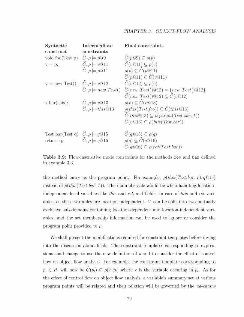
CHAPTER 3. OBJECT-FLOW ANALYSIS
Syntactic Intermediate Final constraintsconstruct constraints
void foo(Test p) C, ρ |= p@9 C(p@9) ⊆ ρ(p)
v = p; C, ρ |= v@11 C(v@11) ⊆ ρ(v)
C, ρ |= p@11 ρ(p) ⊆ C(p@11)
C(p@11) ⊆ C(v@11)
v = new Test(); C, ρ |= v@12 C(v@12) ⊆ ρ(v)
C, ρ |= new Test() C(new Test()@12) = {new Test()@12}C(new Test()@12) ⊆ C(v@12)
v.bar(this); C, ρ |= v@13 ρ(v) ⊆ C(v@13)
C, ρ |= this@13 ρ(this(Test .foo)) ⊆ C(this@13)
C(this@13) ⊆ ρ(param(Test .bar , 1 ))
C(v@13) ⊆ ρ(this(Test .bar))
Test bar(Test q) C, ρ |= q@15 C(q@15) ⊆ ρ(q)
return q; C, ρ |= q@16 ρ(q) ⊆ C(q@16)
C(q@16) ⊆ ρ(ret(Test.bar))
Table 3.9: Flow-insensitive mode constraints for the methods foo and bar definedin example 3.3.
the method entry as the program point. For example, ρ(this(Test .bar , 1 ), q@15)
instead of ρ(this(Test .bar , 1 )). The main obstacle would be when handling location-
independent local variables like this and ret, and fields. In case of this and ret vari-
ables, as these variables are location independent, V can be split into two mutually
exclusive sub-domains containing location-dependent and location-independent vari-
ables, and the set membership information can be used to ignore or consider the
program point provided to ρ.
We shall present the modifications required for constraint templates before diving
into the discussion about fields. The constraint templates corresponding to expres-
sions shall change to use the new definition of ρ and to consider the effect of control
flow on object flow analysis. For example, the constraint template corresponding to
pl ∈ Pv will now be C(pl) ⊆ ρ(x, pl) where x is the variable occuring in pl. As for
the effect of control flow on object flow analysis, a variable’s summary set at various
program points will be related and their relation will be governed by the ud-chains
79
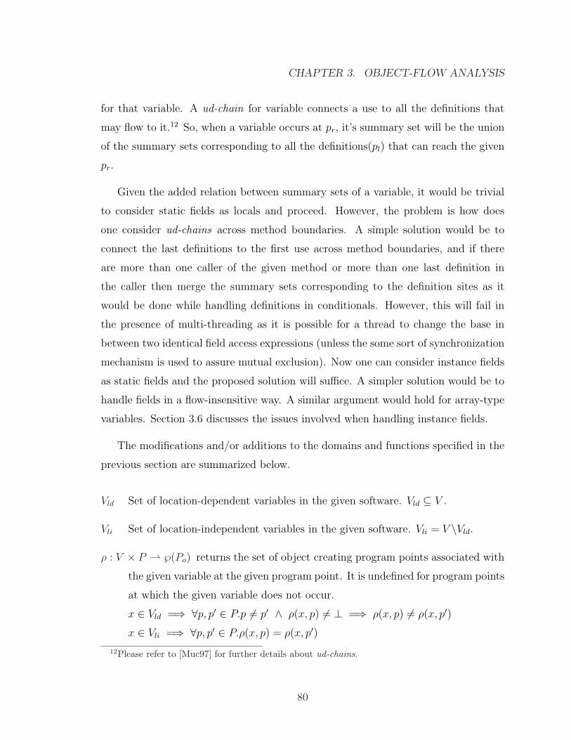
CHAPTER 3. OBJECT-FLOW ANALYSIS
for that variable. A ud-chain for variable connects a use to all the definitions that
may flow to it.12 So, when a variable occurs at pr, it’s summary set will be the union
of the summary sets corresponding to all the definitions(pl) that can reach the given
pr.
Given the added relation between summary sets of a variable, it would be trivial
to consider static fields as locals and proceed. However, the problem is how does
one consider ud-chains across method boundaries. A simple solution would be to
connect the last definitions to the first use across method boundaries, and if there
are more than one caller of the given method or more than one last definition in
the caller then merge the summary sets corresponding to the definition sites as it
would be done while handling definitions in conditionals. However, this will fail in
the presence of multi-threading as it is possible for a thread to change the base in
between two identical field access expressions (unless the some sort of synchronization
mechanism is used to assure mutual exclusion). Now one can consider instance fields
as static fields and the proposed solution will suffice. A simpler solution would be to
handle fields in a flow-insensitive way. A similar argument would hold for array-type
variables. Section 3.6 discusses the issues involved when handling instance fields.
The modifications and/or additions to the domains and functions specified in the
previous section are summarized below.
Vld Set of location-dependent variables in the given software. Vld ⊆ V .
Vli Set of location-independent variables in the given software. Vli = V \Vld.
ρ : V × P ⇀ ℘(Po) returns the set of object creating program points associated with
the given variable at the given program point. It is undefined for program points
at which the given variable does not occur.
x ∈ Vld =⇒ ∀p, p′ ∈ P.p 6= p′ ∧ ρ(x, p) 6= ⊥ =⇒ ρ(x, p) 6= ρ(x, p′)
x ∈ Vli =⇒ ∀p, p′ ∈ P.ρ(x, p) = ρ(x, p′)
12Please refer to [Muc97] for further details about ud-chains.
80
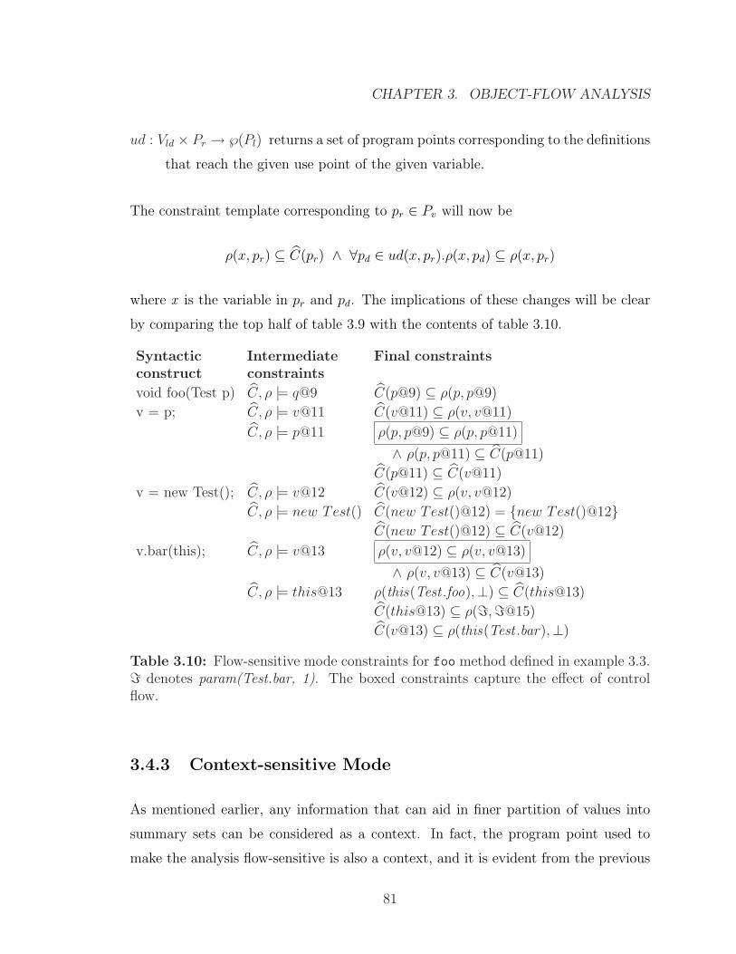
CHAPTER 3. OBJECT-FLOW ANALYSIS
ud : Vld × Pr → ℘(Pl) returns a set of program points corresponding to the definitions
that reach the given use point of the given variable.
The constraint template corresponding to pr ∈ Pv will now be
ρ(x, pr) ⊆ C(pr) ∧ ∀pd ∈ ud(x, pr).ρ(x, pd) ⊆ ρ(x, pr)
where x is the variable in pr and pd. The implications of these changes will be clear
by comparing the top half of table 3.9 with the contents of table 3.10.
Syntactic Intermediate Final constraintsconstruct constraints
void foo(Test p) C, ρ |= q@9 C(p@9) ⊆ ρ(p, p@9)
v = p; C, ρ |= v@11 C(v@11) ⊆ ρ(v, v@11)
C, ρ |= p@11 ρ(p, p@9) ⊆ ρ(p, p@11)
∧ ρ(p, p@11) ⊆ C(p@11)
C(p@11) ⊆ C(v@11)
v = new Test(); C, ρ |= v@12 C(v@12) ⊆ ρ(v, v@12)
C, ρ |= new Test() C(new Test()@12) = {new Test()@12}C(new Test()@12) ⊆ C(v@12)
v.bar(this); C, ρ |= v@13 ρ(v, v@12) ⊆ ρ(v, v@13)
∧ ρ(v, v@13) ⊆ C(v@13)
C, ρ |= this@13 ρ(this(Test .foo),⊥) ⊆ C(this@13)
C(this@13) ⊆ ρ(=,=@15)
C(v@13) ⊆ ρ(this(Test .bar),⊥)
Table 3.10: Flow-sensitive mode constraints for foo method defined in example 3.3.= denotes param(Test.bar, 1). The boxed constraints capture the effect of controlflow.
3.4.3 Context-sensitive Mode
As mentioned earlier, any information that can aid in finer partition of values into
summary sets can be considered as a context. In fact, the program point used to
make the analysis flow-sensitive is also a context, and it is evident from the previous
81
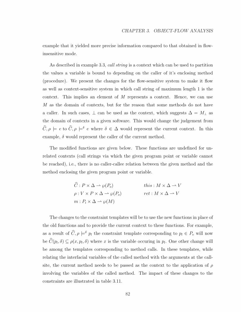
CHAPTER 3. OBJECT-FLOW ANALYSIS
example that it yielded more precise information compared to that obtained in flow-
insensitive mode.
As described in example 3.3, call string is a context which can be used to partition
the values a variable is bound to depending on the caller of it’s enclosing method
(procedure). We present the changes for the flow-sensitive system to make it flow
as well as context-sensitive system in which call string of maximum length 1 is the
context. This implies an element of M represents a context. Hence, we can use
M as the domain of contexts, but for the reason that some methods do not have
a caller. In such cases, ⊥ can be used as the context, which suggests ∆ = M⊥ as
the domain of contexts in a given software. This would change the judgement from
C, ρ |= e to C, ρ |=δ e where δ ∈ ∆ would represent the current context. In this
example, δ would represent the caller of the current method.
The modified functions are given below. These functions are undefined for un-
related contexts (call strings via which the given program point or variable cannot
be reached), i.e., there is no caller-callee relation between the given method and the
method enclosing the given program point or variable.
C : P ×∆ ⇀ ℘(Po) this : M ×∆ ⇀ V
ρ : V × P ×∆ ⇀ ℘(Po) ret : M ×∆ ⇀ V
m : Pi ×∆ ⇀ ℘(M)
The changes to the constraint templates will be to use the new functions in place of
the old functions and to provide the current context to these functions. For example,
as a result of C, ρ |=δ pl the constraint template corresponding to pl ∈ Pv will now
be C(pl, δ) ⊆ ρ(x, pl, δ) where x is the variable occuring in pl. One other change will
be among the templates corresponding to method calls. In these templates, while
relating the interfacial variables of the called method with the arguments at the call-
site, the current method needs to be passed as the context to the application of ρ
involving the variables of the called method. The impact of these changes to the
constraints are illustrated in table 3.11.
82
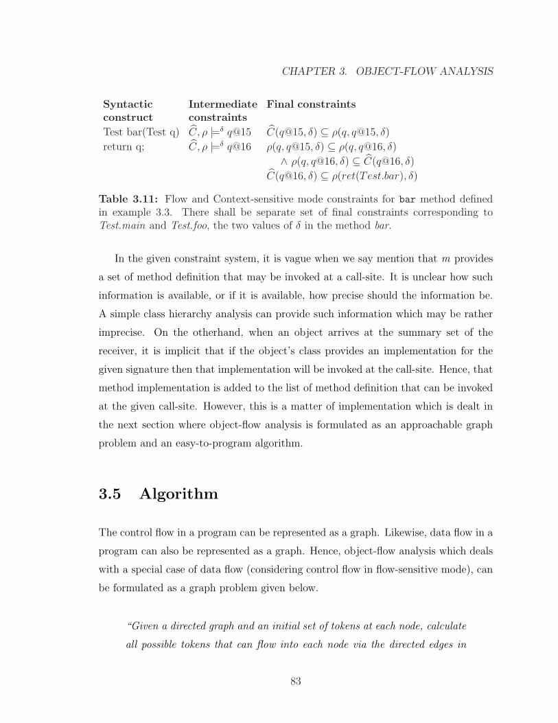
CHAPTER 3. OBJECT-FLOW ANALYSIS
Syntactic Intermediate Final constraintsconstruct constraints
Test bar(Test q) C, ρ |=δ q@15 C(q@15, δ) ⊆ ρ(q, q@15, δ)
return q; C, ρ |=δ q@16 ρ(q, q@15, δ) ⊆ ρ(q, q@16, δ)
∧ ρ(q, q@16, δ) ⊆ C(q@16, δ)
C(q@16, δ) ⊆ ρ(ret(Test.bar), δ)
Table 3.11: Flow and Context-sensitive mode constraints for bar method definedin example 3.3. There shall be separate set of final constraints corresponding toTest.main and Test.foo, the two values of δ in the method bar.
In the given constraint system, it is vague when we say mention that m provides
a set of method definition that may be invoked at a call-site. It is unclear how such
information is available, or if it is available, how precise should the information be.
A simple class hierarchy analysis can provide such information which may be rather
imprecise. On the otherhand, when an object arrives at the summary set of the
receiver, it is implicit that if the object’s class provides an implementation for the
given signature then that implementation will be invoked at the call-site. Hence, that
method implementation is added to the list of method definition that can be invoked
at the given call-site. However, this is a matter of implementation which is dealt in
the next section where object-flow analysis is formulated as an approachable graph
problem and an easy-to-program algorithm.
3.5 Algorithm
The control flow in a program can be represented as a graph. Likewise, data flow in a
program can also be represented as a graph. Hence, object-flow analysis which deals
with a special case of data flow (considering control flow in flow-sensitive mode), can
be formulated as a graph problem given below.
“Given a directed graph and an initial set of tokens at each node, calculate
all possible tokens that can flow into each node via the directed edges in
83
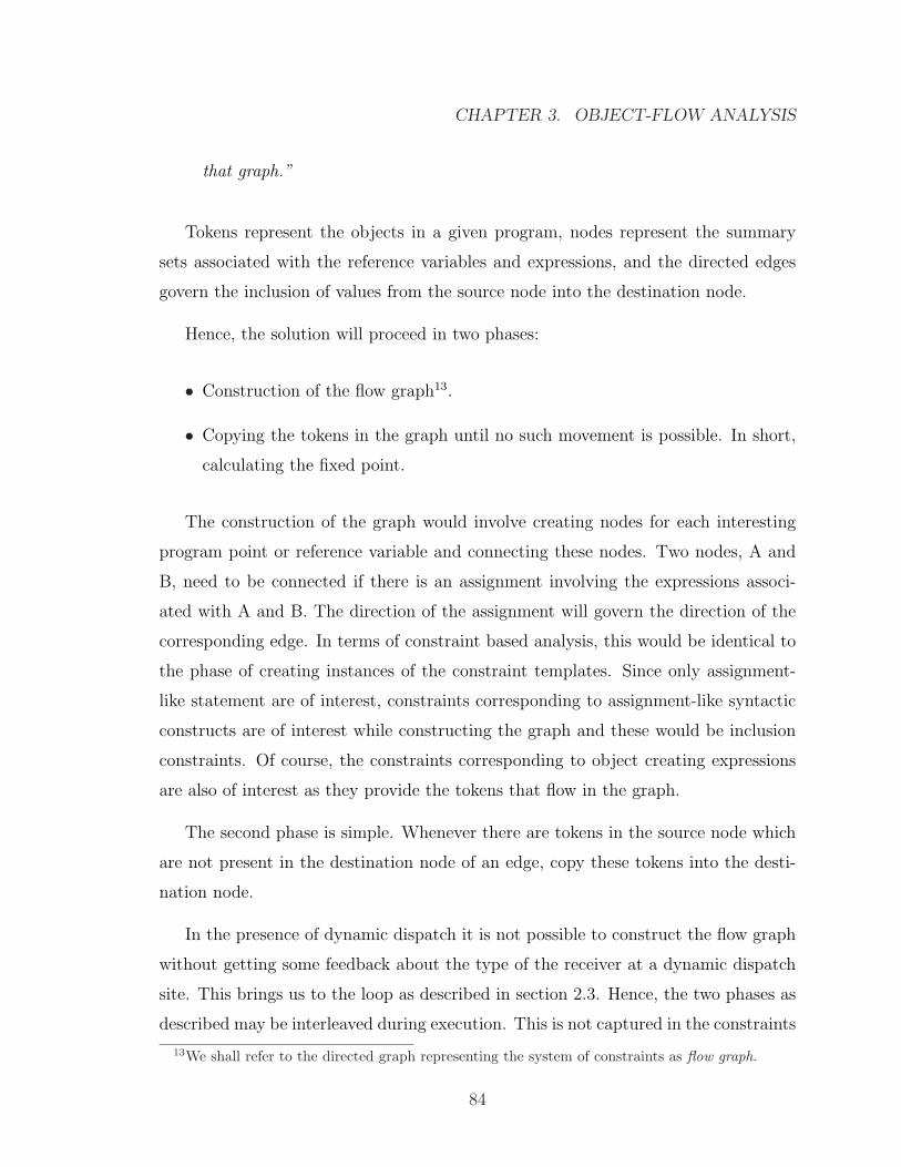
CHAPTER 3. OBJECT-FLOW ANALYSIS
that graph.”
Tokens represent the objects in a given program, nodes represent the summary
sets associated with the reference variables and expressions, and the directed edges
govern the inclusion of values from the source node into the destination node.
Hence, the solution will proceed in two phases:
• Construction of the flow graph13.
• Copying the tokens in the graph until no such movement is possible. In short,
calculating the fixed point.
The construction of the graph would involve creating nodes for each interesting
program point or reference variable and connecting these nodes. Two nodes, A and
B, need to be connected if there is an assignment involving the expressions associ-
ated with A and B. The direction of the assignment will govern the direction of the
corresponding edge. In terms of constraint based analysis, this would be identical to
the phase of creating instances of the constraint templates. Since only assignment-
like statement are of interest, constraints corresponding to assignment-like syntactic
constructs are of interest while constructing the graph and these would be inclusion
constraints. Of course, the constraints corresponding to object creating expressions
are also of interest as they provide the tokens that flow in the graph.
The second phase is simple. Whenever there are tokens in the source node which
are not present in the destination node of an edge, copy these tokens into the desti-
nation node.
In the presence of dynamic dispatch it is not possible to construct the flow graph
without getting some feedback about the type of the receiver at a dynamic dispatch
site. This brings us to the loop as described in section 2.3. Hence, the two phases as
described may be interleaved during execution. This is not captured in the constraints
13We shall refer to the directed graph representing the system of constraints as flow graph.
84
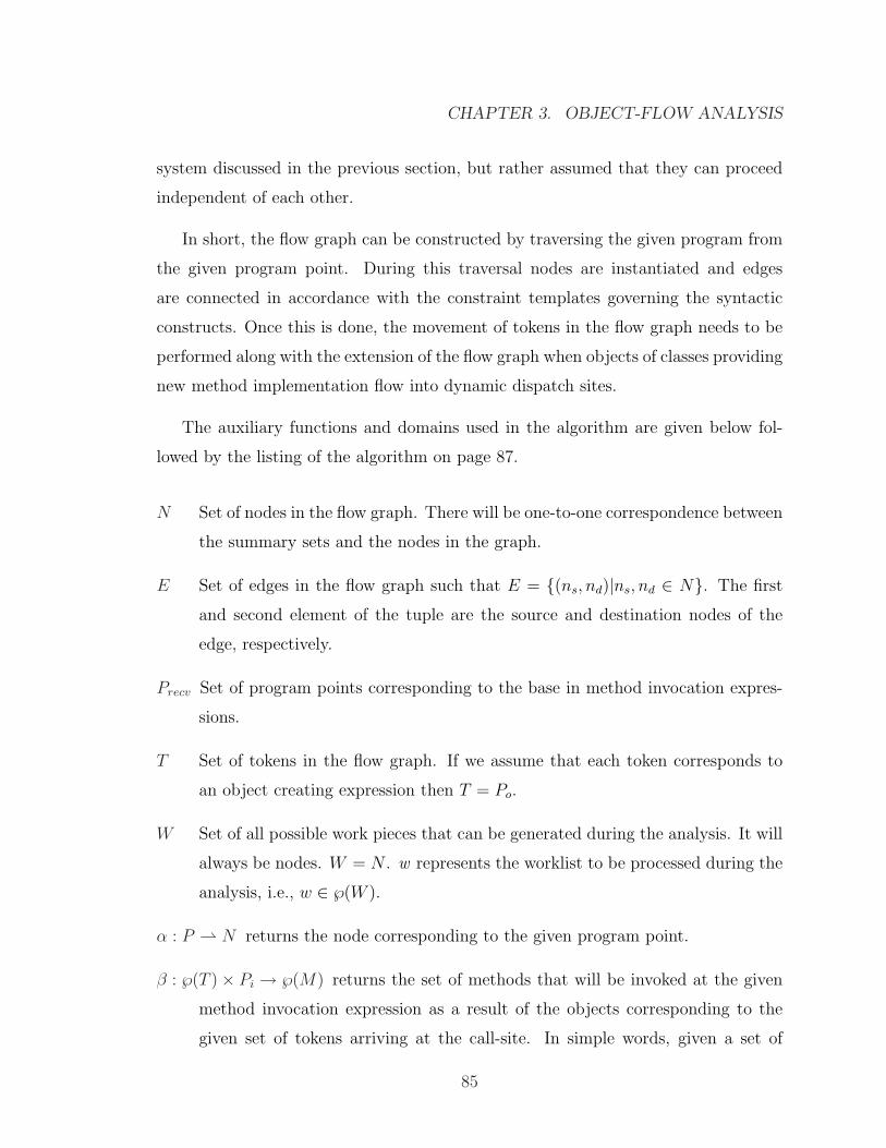
CHAPTER 3. OBJECT-FLOW ANALYSIS
system discussed in the previous section, but rather assumed that they can proceed
independent of each other.
In short, the flow graph can be constructed by traversing the given program from
the given program point. During this traversal nodes are instantiated and edges
are connected in accordance with the constraint templates governing the syntactic
constructs. Once this is done, the movement of tokens in the flow graph needs to be
performed along with the extension of the flow graph when objects of classes providing
new method implementation flow into dynamic dispatch sites.
The auxiliary functions and domains used in the algorithm are given below fol-
lowed by the listing of the algorithm on page 87.
N Set of nodes in the flow graph. There will be one-to-one correspondence between
the summary sets and the nodes in the graph.
E Set of edges in the flow graph such that E = {(ns, nd)|ns, nd ∈ N}. The first
and second element of the tuple are the source and destination nodes of the
edge, respectively.
Precv Set of program points corresponding to the base in method invocation expres-
sions.
T Set of tokens in the flow graph. If we assume that each token corresponds to
an object creating expression then T = Po.
W Set of all possible work pieces that can be generated during the analysis. It will
always be nodes. W = N . w represents the worklist to be processed during the
analysis, i.e., w ∈ ℘(W ).
α : P ⇀ N returns the node corresponding to the given program point.
β : ℘(T )× Pi → ℘(M) returns the set of methods that will be invoked at the given
method invocation expression as a result of the objects corresponding to the
given set of tokens arriving at the call-site. In simple words, given a set of
85
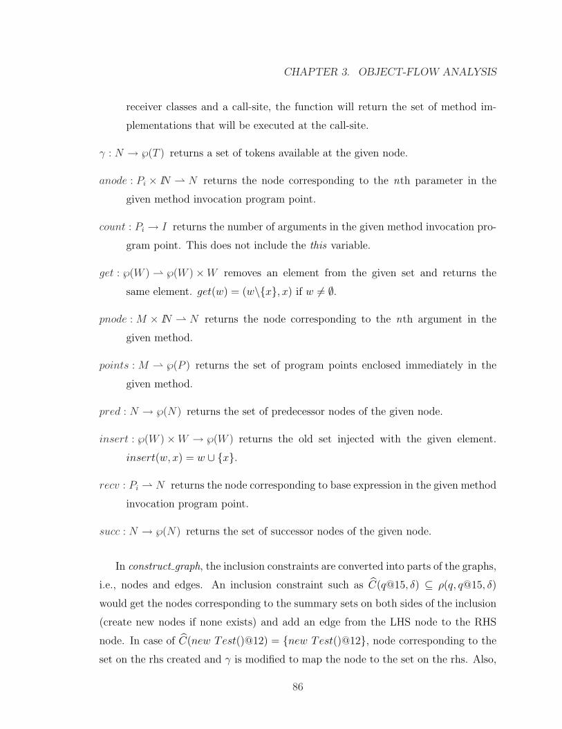
CHAPTER 3. OBJECT-FLOW ANALYSIS
receiver classes and a call-site, the function will return the set of method im-
plementations that will be executed at the call-site.
γ : N → ℘(T ) returns a set of tokens available at the given node.
anode : Pi × IN ⇀ N returns the node corresponding to the nth parameter in the
given method invocation program point.
count : Pi → I returns the number of arguments in the given method invocation pro-
gram point. This does not include the this variable.
get : ℘(W ) ⇀ ℘(W )×W removes an element from the given set and returns the
same element. get(w) = (w\{x}, x) if w 6= ∅.
pnode : M × IN ⇀ N returns the node corresponding to the nth argument in the
given method.
points : M ⇀ ℘(P ) returns the set of program points enclosed immediately in the
given method.
pred : N → ℘(N) returns the set of predecessor nodes of the given node.
insert : ℘(W )×W → ℘(W ) returns the old set injected with the given element.
insert(w, x) = w ∪ {x}.
recv : Pi ⇀ N returns the node corresponding to base expression in the given method
invocation program point.
succ : N → ℘(N) returns the set of successor nodes of the given node.
In construct graph, the inclusion constraints are converted into parts of the graphs,
i.e., nodes and edges. An inclusion constraint such as C(q@15, δ) ⊆ ρ(q, q@15, δ)
would get the nodes corresponding to the summary sets on both sides of the inclusion
(create new nodes if none exists) and add an edge from the LHS node to the RHS
node. In case of C(new Test()@12) = {new Test()@12}, node corresponding to the
set on the rhs created and γ is modified to map the node to the set on the rhs. Also,
86
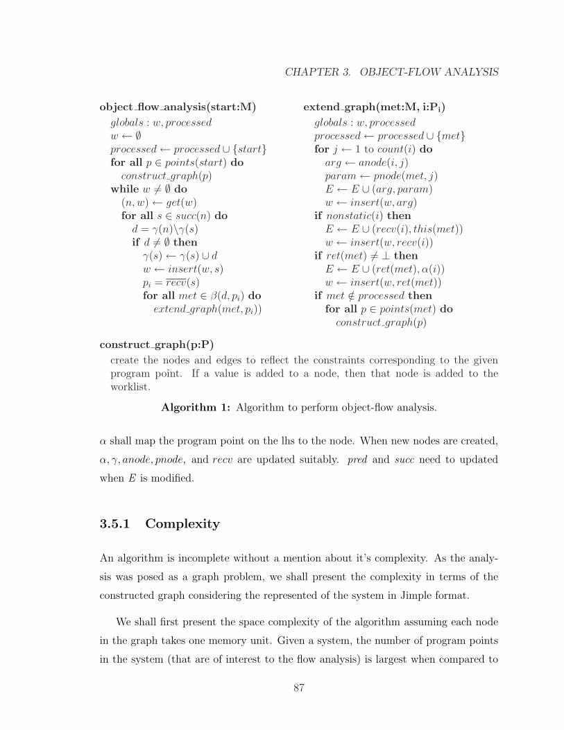
CHAPTER 3. OBJECT-FLOW ANALYSIS
object flow analysis(start:M)
globals : w, processedw ← ∅processed← processed ∪ {start}for all p ∈ points(start) do
construct graph(p)while w 6= ∅ do
(n,w)← get(w)for all s ∈ succ(n) do
d = γ(n)\γ(s)if d 6= ∅ then
γ(s)← γ(s) ∪ dw ← insert(w, s)pi = recv(s)for all met ∈ β(d, pi) do
extend graph(met, pi))
extend graph(met:M, i:Pi)
globals : w, processedprocessed← processed ∪ {met}for j ← 1 to count(i) do
arg ← anode(i, j)param← pnode(met, j)E ← E ∪ (arg, param)w ← insert(w, arg)
if nonstatic(i) thenE ← E ∪ (recv(i), this(met))w ← insert(w, recv(i))
if ret(met) 6= ⊥ thenE ← E ∪ (ret(met), α(i))w ← insert(w, ret(met))
if met /∈ processed thenfor all p ∈ points(met) do
construct graph(p)
construct graph(p:P)
create the nodes and edges to reflect the constraints corresponding to the givenprogram point. If a value is added to a node, then that node is added to theworklist.
Algorithm 1: Algorithm to perform object-flow analysis.
α shall map the program point on the lhs to the node. When new nodes are created,
α, γ, anode, pnode, and recv are updated suitably. pred and succ need to updated
when E is modified.
3.5.1 Complexity
An algorithm is incomplete without a mention about it’s complexity. As the analy-
sis was posed as a graph problem, we shall present the complexity in terms of the
constructed graph considering the represented of the system in Jimple format.
We shall first present the space complexity of the algorithm assuming each node
in the graph takes one memory unit. Given a system, the number of program points
in the system (that are of interest to the flow analysis) is largest when compared to
87
CHAPTER 3. OBJECT-FLOW ANALYSIS
the number of fields, locals, and array components. Let’s denote these numbers by
np, nf , nl, and nac. In totally insensitive mode, there is 1-1 correspondence between
these numbers and the number of nodes in the graph. Hence, the space complexity in
terms of the number nodes in the graph will be O(np). In case of flow sensitive mode,
there is a 1-n correspondence between nl and the number of nodes corresponding
to locals in the graph. As the increase in the number of nodes corresponds to the
program points at which the locals occur, the increased nl will be comparable (in
most case nl < c×npp) to np. Hence, it is safe to say that the space complexity is still
O(np). A similar argument shall hold in the case of flow and allocation-site sensitive
mode, and hence, the worst-case space complexity of the algorithm in terms of the
number of nodes in the final graph will be O(np).
The time complexity for the algorithm would be the amount of time for the graph
to stabilize. This would mean from the time the first value is injected into the
first node till the time the values cease to flow in the graph. It is known that only
allocation-site expressions in the system flow in the graph. Hence, it is reasonable,
although pessimistic, to say that once all the allocation-site expressions have reached
all the nodes, the algorithm terminates. It is pessimistic because it is usually the case
that not all allocation-site expressions can reach all nodes due to type constraints
and programming logic. Now, if we assume one allocation-site expression would take
a unit of time to be copied from the source to destination node, then the worst-case
time complexity of the algorithm would be na × e where na is the total number of
allocation-site expressions in the system and e is the total number of edges in the
graph.
An interesting twist would be that the graph can grow dynamically. So, given
a system, e is not bound to a static value. A simple solution would be to assume
e is the number of edges in the graph when all plausible method implementations
are considered at call-sites. A more optimistic solution would be to instrument a
function which provides a connectivity index (a positive fraction less than 1) for the
given system in a given mode. If such a function is available, it can be used to
88
CHAPTER 3. OBJECT-FLOW ANALYSIS
predict the number of edges in the flow graph corresponding to a given system in
a given mode. One may argue either way about the feasibility of such a function.
However, if one such function is available, it can help tighten the time complexity of
the algorithm.
3.6 Fields and Arrays
Previous discussions about arrays and fields in various modes of the analysis was
rather elusive. The reason being that one needs to understand the dependency be-
tween various def-use sites across method boundaries and how this is affects the
analysis in terms of precision. In the following discussion, we shall restrict ourselves
to field access expressions of type a.b where a is the primary and b is the identifier.
Similarly, we shall deal with array expressions of the form a[b]. As these two are
the basic forms using which all other complex forms such as a.b.c and a[b][c] can
be represented. All discussions regarding these forms can be trivially extended to
complex forms.
3.6.1 Static Fields
We shall start with static fields. Since they are not bound to any base object, static
fields can be handled as global variables with their fully qualified name helping in
identifying static fields with the same identifier but declared in different classes.
It would be trivial to handle static fields in flow-insensitive mode as there is
no control-flow dependent relation between various occurrences of the fields. On
the other hand, flow-sensitive mode requires various occurrences of the fields to be
related in a way dependent on the control-flow. Speaking intraprocedurally, it may
seem reasonable to use a intraprocedural ud-chain and relate the use of a field to it’s
definition(s). The only drawback being that the field may be defined in a method
which was called en route from the def-site to the use-site. Such modifications are
89
CHAPTER 3. OBJECT-FLOW ANALYSIS
external to the method being analyzed and is across method boundaries. This can be
remedied if the ud-chains were interprocedural, but inter-procedural ud-chains require
a precise call-graph which in our case is progressively available. In simple words, when
a new method defining the field is plugged at a call-site, any definitions of the field
in the new method that may be visible to the external world will need to be added
to the list of definitions that may reach the use-site. Since, the precise call-graph is
progressively constructed it is possible that the as the analysis proceeds the call-graph
expands and discovers a method definition at a call-site along a ud-chain. In such a
case, the call-site kills the previous definition. This implies the contribution of the
previous definition to the use-site must be disregarded to make the analysis precise.
In simple words, as the ud-chains and OFA are interdependent, both need to reach
their fixed point simultaneously for OFA to provide information at the assured level
of precision.
The above solutions will fail in the context of multi-threading as external modifi-
cation of the field may be across thread boundaries, and hence, it cannot be detected
by sequential tracking of control-flow. In the case of static fields, as there is no base or
primary object associated with the field access, even the effect of synchronization can-
not contribute to the solution. This indicates that in the context of multi-threading
static fields are harder to handle than instance fields.
3.6.2 Instance Fields
Instance fields are associated with particular objects and this adds a new dimension
to the problem of tracking the flow of objects through instance fields. The simplest
solution to tackle the issue of instance fields are by considering them independent of
the objects to which they belong, i.e., instance fields are considered as static fields.
This is overly conservative.
The precision can be improved if the previous summary set can be divided based
on the object creation site of the object via which the field is being accessed in the
90
CHAPTER 3. OBJECT-FLOW ANALYSIS
field access expression. In simple words, the set of objects a field can refer to when
accessed via an object created at an object creation site is more precise. Consider
the following snippet of code in which f is an instance field of class A, and x and y
are variables of type A. It is evident from the code that x.f and y.f need not have
the same summary sets as they are being accessed via two different objects created
at lines 1 and 3, respectively.14
1 x = new A();2 x. f = j;3 y = new A();4 y. f = k;
Hence, considering object creation site as a context improves the precision of OFA
information corresponding to instance fields. The next improvement would be to make
the information flow-sensitive using the summary set associated with the primary in
the field access expression. A simple minded approach would be to create ud-chains
such that the primaries at the def- and use-sites in each ud-chain need to be identical.
The drawback with this approach is that, at run-time, when the control reaches the
use-site from the def-site, it is possible that the primary at the def-site may not refer
to the same object as the primary at the use-site. Hence, an improved solution would
be to require that the primaries at the def- and use-sites need to refer to the same
object creation site for the sites to appear in the ud-chain corresponding to the field
access expression. Although this solution seems correct, it fails in the case where the
object creation site is enclosed in a loop, i.e., an object creation site may create more
than object at run-time and the primaries at the def- and use-sites may refer to two
such different objects created at the same object creation site. So, a correct solution
would be to require that the primaries at the def- and use-sites need to refer to the
same object for the sites to appear in the ud-chain corresponding to the field access
expression. The same reason makes it hard to generate summary sets for instance
fields of each object created in the given software.
A simple symbolic analysis can provide the information if two variables evaluate
14Although it is possible that their summary sets may be identical because the summary sets ofj and k may be identical.
91
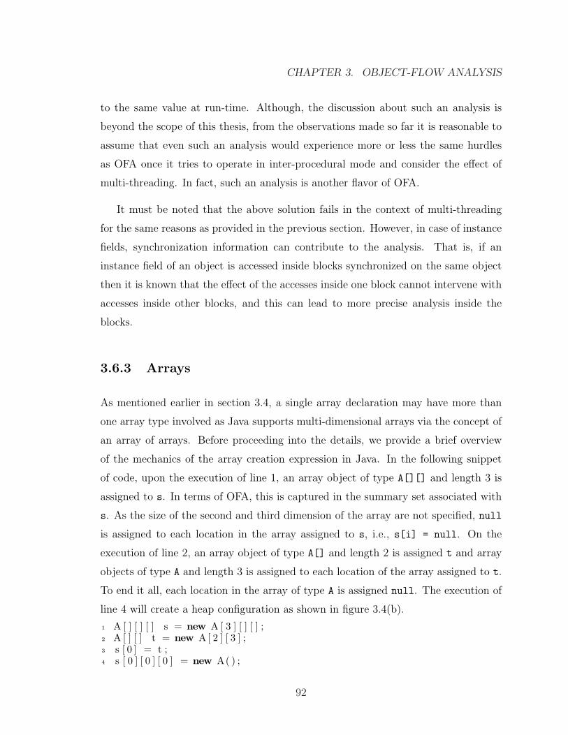
CHAPTER 3. OBJECT-FLOW ANALYSIS
to the same value at run-time. Although, the discussion about such an analysis is
beyond the scope of this thesis, from the observations made so far it is reasonable to
assume that even such an analysis would experience more or less the same hurdles
as OFA once it tries to operate in inter-procedural mode and consider the effect of
multi-threading. In fact, such an analysis is another flavor of OFA.
It must be noted that the above solution fails in the context of multi-threading
for the same reasons as provided in the previous section. However, in case of instance
fields, synchronization information can contribute to the analysis. That is, if an
instance field of an object is accessed inside blocks synchronized on the same object
then it is known that the effect of the accesses inside one block cannot intervene with
accesses inside other blocks, and this can lead to more precise analysis inside the
blocks.
3.6.3 Arrays
As mentioned earlier in section 3.4, a single array declaration may have more than
one array type involved as Java supports multi-dimensional arrays via the concept of
an array of arrays. Before proceeding into the details, we provide a brief overview
of the mechanics of the array creation expression in Java. In the following snippet
of code, upon the execution of line 1, an array object of type A[][] and length 3 is
assigned to s. In terms of OFA, this is captured in the summary set associated with
s. As the size of the second and third dimension of the array are not specified, null
is assigned to each location in the array assigned to s, i.e., s[i] = null. On the
execution of line 2, an array object of type A[] and length 2 is assigned t and array
objects of type A and length 3 is assigned to each location of the array assigned to t.
To end it all, each location in the array of type A is assigned null. The execution of
line 4 will create a heap configuration as shown in figure 3.4(b).
1 A [ ] [ ] [ ] s = new A [ 3 ] [ ] [ ] ;2 A [ ] [ ] t = new A[ 2 ] [ 3 ] ;3 s [ 0 ] = t ;4 s [ 0 ] [ 0 ] [ 0 ] = new A( ) ;
92
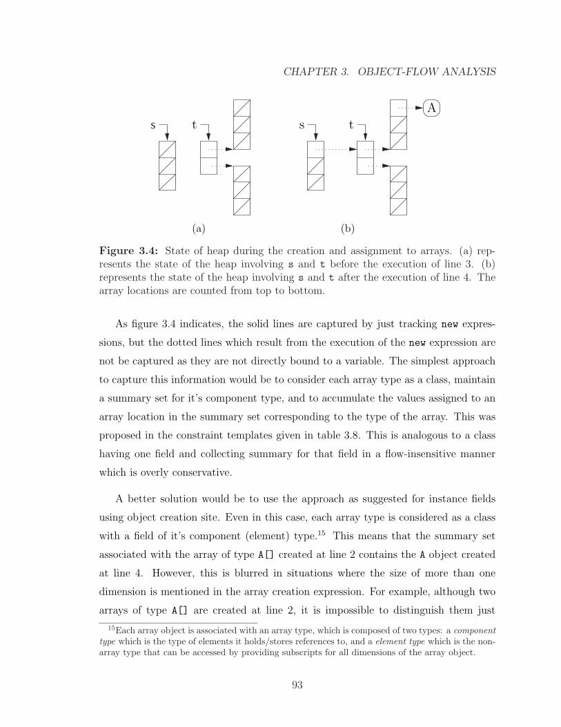
CHAPTER 3. OBJECT-FLOW ANALYSIS
sA
t s t
(a) (b)
Figure 3.4: State of heap during the creation and assignment to arrays. (a) rep-resents the state of the heap involving s and t before the execution of line 3. (b)represents the state of the heap involving s and t after the execution of line 4. Thearray locations are counted from top to bottom.
As figure 3.4 indicates, the solid lines are captured by just tracking new expres-
sions, but the dotted lines which result from the execution of the new expression are
not be captured as they are not directly bound to a variable. The simplest approach
to capture this information would be to consider each array type as a class, maintain
a summary set for it’s component type, and to accumulate the values assigned to an
array location in the summary set corresponding to the type of the array. This was
proposed in the constraint templates given in table 3.8. This is analogous to a class
having one field and collecting summary for that field in a flow-insensitive manner
which is overly conservative.
A better solution would be to use the approach as suggested for instance fields
using object creation site. Even in this case, each array type is considered as a class
with a field of it’s component (element) type.15 This means that the summary set
associated with the array of type A[] created at line 2 contains the A object created
at line 4. However, this is blurred in situations where the size of more than one
dimension is mentioned in the array creation expression. For example, although two
arrays of type A[] are created at line 2, it is impossible to distinguish them just
15Each array object is associated with an array type, which is composed of two types: a componenttype which is the type of elements it holds/stores references to, and a element type which is the non-array type that can be accessed by providing subscripts for all dimensions of the array object.
93
CHAPTER 3. OBJECT-FLOW ANALYSIS
considering their creation site. Although, the index may help here, further analysis
in terms of indices is hard to achieve as the subscripts can be expressions that need to
be evaluated at run-time, and this would require a much costlier analysis to determine
the indices.
The drawbacks mentioned in the previous section in the context of multi-threading
hold here, too.
3.6.4 Observations
An observation considering static analyses is that such analyses usually depend on
other static analyses of the similar nature. As these analyses provide a solution via
reaching a fixed point, the question is, “would it be better if each analysis is repeated
till all of the involved analyses reach a fixed point (similar to chaotic iteration) or to
device an analysis that embodies all the involved analyses and require this analysis
to reach a fixed point?” Either way it’s a matter of reaching a fixed point, either
individually first, but simultaneously, or cumulatively. Our experience indicates that
the former approach would be extensible while the former would be faster.
Another interesting observation is that the static analyses proceed from intra-
procedural to inter-procedural mode, i.e., in an incremental manner in terms of the
composition of the given software. Similarly, the precision improves incrementally
in terms of composition of the given software. Inter-procedural mode of analysis
provides more precise information compared to intra-procedural analysis. This rises
the question, “would incremental and staged flavor of static analyses improve the
precision and also the cost of analyses?” We do not have any data in this regard to
provide an opinion, but by intuition and observation, it seems that incremental and
staged flavor of static analyses may be more effective in terms of performance.
94
Chapter 4
The Implementation
This chapter starts by presenting the environment in which the implementation of
object flow analysis will execute, and the framework providing the intermediate rep-
resentation used in the analysis. It then details the general framework, Bandera Flow
Analysis(BFA) framework, using which OFA(Object-Flow Analysis) has been realized.
4.1 Bandera
As already mentioned, Bandera[CDH+00] is a tool set for verifying software written
in Java using model checking techniques. This is the product of an on-going project
by the same name at Kansas State University, USA.
The tool set has a collection of tools working in tandem as depicted in the fig-
ure 4.1. The components of the tool set can be arranged as a pipeline divided into
3 sections. The first section is similar to the front-ends of a compiler. It operates
on Java source code and the intermediate representation. Java-to-Jimple-to-Java
Compiler (JJJC) compiles the Java source code into Jimple1, the intermediate repre-
sentation (IR), and also bears the responsibility of mapping the pieces of jimple back
1please refer to the next section for details on jimple.
95
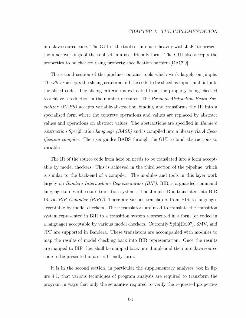
CHAPTER 4. THE IMPLEMENTATION
into Java source code. The GUI of the tool set interacts heavily with JJJC to present
the inner workings of the tool set in a user-friendly form. The GUI also accepts the
properties to be checked using property specification patterns[DAC99].
The second section of the pipeline contains tools which work largely on jimple.
The Slicer accepts the slicing criterion and the code to be sliced as input, and outputs
the sliced code. The slicing criterion is extracted from the property being checked
to achieve a reduction in the number of states. The Bandera Abstraction-Based Spe-
cializer (BABS) accepts variable-abstraction binding and transforms the IR into a
specialized form where the concrete operations and values are replaced by abstract
values and operations on abstract values. The abstractions are specified in Bandera
Abstraction Specification Language (BASL) and is compiled into a library via A Spec-
ification compiler. The user guides BABS through the GUI to bind abstractions to
variables.
The IR of the source code from here on needs to be translated into a form accept-
able by model checkers. This is achieved in the third section of the pipeline, which
is similar to the back-end of a compiler. The modules and tools in this layer work
largely on Bandera Intermediate Representation (BIR). BIR is a guarded command
language to describe state transition systems. The Jimple IR is translated into BIR
IR via BIR Compiler (BIRC). There are various translators from BIR to languages
acceptable by model checkers. These translators are used to translate the transition
system represented in BIR to a transition system represented in a form (or coded in
a language) acceptable by various model checkers. Currently Spin[Hol97], SMV, and
JPF are supported in Bandera. These translators are accompanied with modules to
map the results of model checking back into BIR representation. Once the results
are mapped to BIR they shall be mapped back into Jimple and then into Java source
code to be presented in a user-friendly form.
It is in the second section, in particular the supplementary analyses box in fig-
ure 4.1, that various techniques of program analysis are required to transform the
program in ways that only the semantics required to verify the requested properties
96
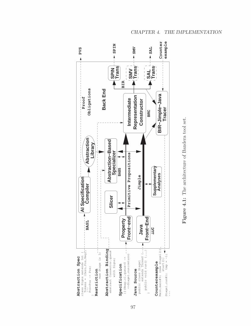
CHAPTER 4. THE IMPLEMENTATION
Rep
rese
nta
tio
nIn
term
edia
te
Co
nst
ruct
or
SM
VT
ran
s
SP
INT
ran
s
SA
LT
ran
s
Ab
stra
ctio
nL
ibra
ry
Su
pp
lem
enta
ryA
nal
yses
Proof
Obligations
Co
mp
iler
AI S
pec
ific
atio
n
Pro
per
tyF
ron
t−en
d
Counter
example
[](Heap.c1.queue>0 −>
<>Stage1.run:return)
...
Stage1.run#1: tmp = −1;
start();
Main.main#3: (new Stage1()).
} extends Thread {
public void run() {...}
public class Stage1
class Signs extends Int {
Tokens = {Zero,Pos,Neg};
...
Pos+Pos −> Pos;
}
abstract Connector.queue
with Signs;
SAL
SMV
BIR
−Jim
ple
−Jav
aT
race
r
Slic
erS
pec
ializ
erA
bst
ract
ion
−Bas
ed
BASL
Fro
nt−
En
dJa
va
Primitive Propositions
JJJC
Jimple
PVS
BABS
BIRC
Bac
k E
nd
BIR
SPIN
Abstraction Spec
Restriction
Specification
Java Source
Counterexample
max Stage is 3;
Abstraction Binding
Fig
ure
4.1
:T
he
arch
itec
ture
ofB
ander
ato
olse
t.
97
CHAPTER 4. THE IMPLEMENTATION
are retained to provide a concise and precise model. By doing so, the requested
property can be verified in a reasonable, even short, amount of time. As mentioned
previously, slicing and abstraction are two such techniques, and slicing can benefit
from object-flow information.
4.2 Soot
Soot[VR00] is a Java bytecode optimization framework designed by Raja Vallee-Rai
in McGill University, Canada. This framework works on bytecodes in Java class files,
and hence, is language independent. The class files can be represented in memory in
any of the following 3 intermediate representations.
BAF This is a stack-based IR of Java byte code with a set of orthogonal instructions.
It is the most basic representation available in the SOOT framework and is
suitable for analyses and transformations that must be performed on stack code.
Jimple This is a typed and compact 3-address code representation of the bytecode.
Optimizing stack code, untyped nature of variables, and the separation of local
and stack based variables in the bytecode were the motivation for this rep-
resentation. This representation is ideal for performing various analyses and
optimization of class files.
Grimp This representation allows for tree of expressions as opposed to flat expres-
sions in Jimple. The motivation behind this representation was the readability
of IR which is lost due to too many goto’s and extremely fragmented expressions.
This representation when viewed looks similar to decompiled Java bytecodes.
Once the class files are represented in memory in one of the above forms it can be easily
translated into any of the other two forms. This means once the class file is loaded, it’s
representation can be changed as required by the transformation being applied. Once
done with the transformations, bytecodes can be generated by traversing the Grimp
98
CHAPTER 4. THE IMPLEMENTATION
or BAF representation. The framework is also accompanied with some analyses that
can be used to optimize the representation when it gets translated from one IR to
another.
4.2.1 Jimple
The merits of Jimple as presented above and as in [VR00] make it the ideal candidate
to be used as an intermediate representation for various analysis and transformation.
As Jimple is an IR, Java source code can be compiled into Jimple representation.
Also, SOOT provides facility to create Jimple representation from class files. Hence,
Jimple is an ideal choice to represent systems in which Java class libraries are used
and the source code for these libraries is not available. This is the part of the classic
problem of trying to represent a system in it’s entirety even when the entities involved
in the system are not available in a common form. However, this does not provide an
easy solution in cases when a system written in Java can uses a library written in C.
Jimple representation is composed of instances of Value and Unit classes. Value
represents entities that yield values on execution. In simple words, they are expres-
sions, constants, and various types of variable references. On the other hand, Unit
represents entities that do not yield values but may cause side effects. In simple
words, they are statements. Unit and Value have various sub-classes which provide
specialized behaviors corresponding to the type of expression or statement they repre-
sent. For example, AssignStmt objects represent assignment statements, and the lhs
and rhs are represented as Value objects. Similarly, VirtualInvokeExpr represents
a virtualinvoke bytecode with all the required arguments. As Jimple representa-
tion can be generated from class files, it is closely modeled on the Java bytecodes
as specified in [LY99]. Hence, the subclasses of Value and Unit have more or less
one-to-one correspondence with the Java bytecodes.
It should be noted that various occurrences of a semantic entity is captuted by
boxes. Jimple uses a notion of box in the AST as place holders for the actual entities.
99
CHAPTER 4. THE IMPLEMENTATION
The boxes contain the information regarding which entity occurs at that location in
the AST. There are two types of boxes in Jimple: UnitBox and ValueBox. The latter
is of importance in flow-sensitive mode of OFA.
Soot provides SootClassManager class which manages the classes. It acts like
a repository of classes. A Java class is represented by an instance of SootClass.
Each such instances encapsulates the attributes and their properties as instances
of SootField, and each method of the Java class as instances of SootMethod.
SootMethod objects encapsulate the representation of the method as an instance
of Body. There are several subclasses of the Body class. These subclasses are specific
to the representations discussed in section 4.2, and hence, in the common framework
the logic of a system can be represented in three forms. JimpleBody is one such
form which embodies the Jimple representation of the method. There shall be no
Body associated with the SootMethod if the method is a native method. This may be
considered as the extent to which Soot may be used to address the problem of closing
a system. It is also interesting to note that these classes in Soot model the constant
pool and it’s characteristics as represented in a class file.
There are certain implications of using Jimple. Since Jimple represents bytecodes,
there may be more than one piece of Jimple code corresponding to a single piece of
Java code. This means it is the responsibility of the external environment to maintain
the mapping between Java source code and it’s Jimple representation. Also, it is
possible that there may be more than one variable in Jimple corresponding to a
single variable in Java. This is controlled by certain parameters which govern how
the representation is built in Jimple. In such cases the external environment must
use SimpleXXXXX classes in ca.mcgill.sable.soot.jimple package to discover the
control relation between various instances of variables in Jimple.
100
CHAPTER 4. THE IMPLEMENTATION
4.3 BFA: The Underlying Framework
Bandera Flow Analysis(BFA) framework is a framework to implementation constraint-
based style flow analyses that work on Jimple representation. It hinges on three con-
cetps, Variants, Managers, and Indices. These three concepts provide the ability to
implement an analysis once and vary it’s precision by mere initialization.
In this section we start by presenting the two basic concepts of BFA and how
they relate to the theory discussed in the previous chapter. This is followed by an
explanation of how the flow analysis framework is implemented and used to realize
object-flow analysis.
4.3.1 Variants
Variants capture the notion of variance of a semantic entity in a given context. For
example, in flow-insensitive mode, all occurrences of a local variable in a method is
represented by the same variant of the variable. However, in flow-sensitive mode, all
occurrences of a local variable in a method are represented by unique variants of the
variable. In terms of the concepts introduced in the previous chapter, each variant
abstracts the summary set associated with a semantic entity in a given context.
In terms of implementation, each type of variant captures some information
about the semantic entity is it representing and the corresponding summary set.
Each type of variant is represented as a class in framework. They are ASTVariant,
ArrayVariant, FieldVariant, and MethodVariant. The first three class are asso-
ciated with semantic entities that are associated with summary sets. Hence, they
extend AbstractValuedVariant class. On the other hand, MethodVariant repre-
sents a variant of a method, and hence, is associated with more than one summary
set. It is contains the variants associated with the AST nodes that occur in the asso-
ciated method. If any, it also contains the variants associated with the this variable,
parameter variables, and the method return value. Both AbstractValuedVariant
101
CHAPTER 4. THE IMPLEMENTATION
and MethodVariant implement Variant, a marker interface. The corresponding class
diagram is given in figure 4.2.
In the previous chapter, we posed the flow of values in the analysis as flow of values
in a graph. In implementation, this is realized via a graph of FGNode which abstract or
represent the summary set. Each AbstractValuedVaraint encapsulates an instance
of FGNode and thereby indirectly encapsulates the summary set. This separates the
information maintained by flow analysis (variants) and information calculated by flow
analysis (summary set). The logic of connecting the nodes are delegated to objects
providing FGNodeConnector interface.
4.3.2 Managers
As presented in the previous chapter, maps from pairs of entities and context to
summary set are maintained during the analysis via mapping functions. These
mapping functions are realised in BFA as Manager classes. There are 4 variant
managing classes in BFA. They are ASTVariantManager, ArrayVariantManager,
FieldVariantManager, and MethodVariantManager. These classes inherit from
AbstractVariantManager which contains the logic to manage the variants. The
subclasses provide the implementation to generate new variants. Each of the man-
ager subclasses implement Prototype interface. This interface is used to realize the
Prototype[GHJV95] design pattern to generate new instances of managers once the
framework has been initialized. The class diagram of managers is given in figure 4.3.
4.3.3 Indices
Indices capture the input to the various mapping functions introduced in the previous
chapter. In simple terms, it abstracts the pair of semantic entity and context provided
as input mapping functions such as ρ and C. For example, given a local variable and
a context, the corresponding index will uniquely identify the corresponding Variant.
102
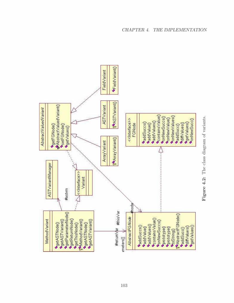
CHAPTER 4. THE IMPLEMENTATION
Fig
ure
4.2
:T
he
clas
sdia
gram
ofva
rian
ts.
103
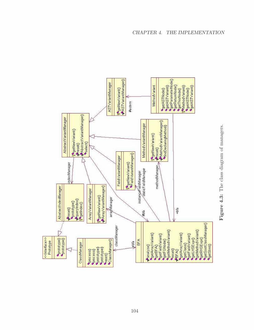
CHAPTER 4. THE IMPLEMENTATION
Fig
ure
4.3
:T
he
clas
sdia
gram
ofm
anag
ers.
104
CHAPTER 4. THE IMPLEMENTATION
This encapsulates the schemes to uniquely identify variants in various mode. The
programmer would provide an implementation to generate a unique index representing
the given entity and context, and this implementation would be used seamlessly to
run the analysis in the required mode.
In terms of implementation, at present, the framework supports the combi-
nation of flow-sensitive and flow-insensitive modes with allocation-site insensitive
and allocation-site sensitive modes. These modes are achieved via extension of
AbstractIndexManager class. This class implements Prototype for similar reasons
presented earlier. Currently, there are 3 extensions of AbstractIndexManager. The
first being modes.insensitive.IndexManager class provides implementation to gen-
erate indices in both in-sensitive mode. It can be used in any in-sensitive mode as
it discards any context information while generating the indices. The second and
third extensions are modes.sensitive.AllocationSiteSensitiveIndexManager
and modes.sensitive.FlowSensitiveASTIndexManager classes which provide
the indices in flow-sensitive and allocation-site sensitive modes, respectively.
Both, these managers provide as indices objects of classes which extend
modes.sensitive.OneContextInfoIndex class. OneContextInfoClass encapsu-
lates one chunk of context information, i.e., the program point in flow-sensitive mode
and the allocation-site in allocation-site sensitive mode.
4.3.4 The Framework
The framework consists of a run-time central repository of instances of flow analyses
represented by BFA class. BFA connects the various components in the framework
and also provides an interface to extract low-level flow analysis information. It also
encapsulates a ModeFactory object which provides mode specific components when
constructing an instance of an analysis. Internally, ModeFactory uses object providing
Prototype interface to provide mode specific components.
The low-level information provided via BFA’s interface may be too fine grained
105
CHAPTER 4. THE IMPLEMENTATION
in most occasions. Some sort of post processing would make the information more
accessible to the clients. Hence, AbstractAnalyzer class can be specialized to pro-
vided more refined information to the clients. The rationale for such a design is that
the clients interested in the set of method implementation that can be invoked at a
call-site will not be interested in the set of objects a primary evaluates in the method
invocation expression. Rather the clients would just want to provide the invoca-
tion expression and want a set of methods in return. This simplifies the interaction
between the clients and the analysis.
Other classes of interest in the framework are AbstractExprSwitch,
AbstractStmtSwitch, AbstractWork, Context, and WorkList. The first two classes
realize a Visitor [GHJV95] pattern for expressions and statements in Jimple2. The
programmer will deal with FGNode in these classes as they provide the logic to con-
struct the flow graph. AbstractWork and WorkList provide the interface and im-
plementation to realize the worklist algorithm. Context encapsulates teh context
information during the analysis. The class diagram for the framework is given in
figure 4.4.
An instance of the framework would provide analysis specific implementa-
tion of expression and statement visitors by extending AbstractExprSwitch and
AbstractStmtSwitch. It will also provide analysis specific specialization of FGNode
and AbstractWork classes. If the instance functions in a mode other than the one
provided by BFA, the programmer will also provide mode specific index managers.
Once the specialized analyzer object is created with prototypical instances of various
components, the instance is ready to analyze and provide results.
4.4 OFA: An Instance of BFA
Object Flow Analysis(OFA) as described in this thesis is realized through the BFA
framework. It is realized by implementing 15 classes. OFA is implemented in all the
2In reality, they are visitors capable of walking over Jimple extensions introduced by Bandera.
106
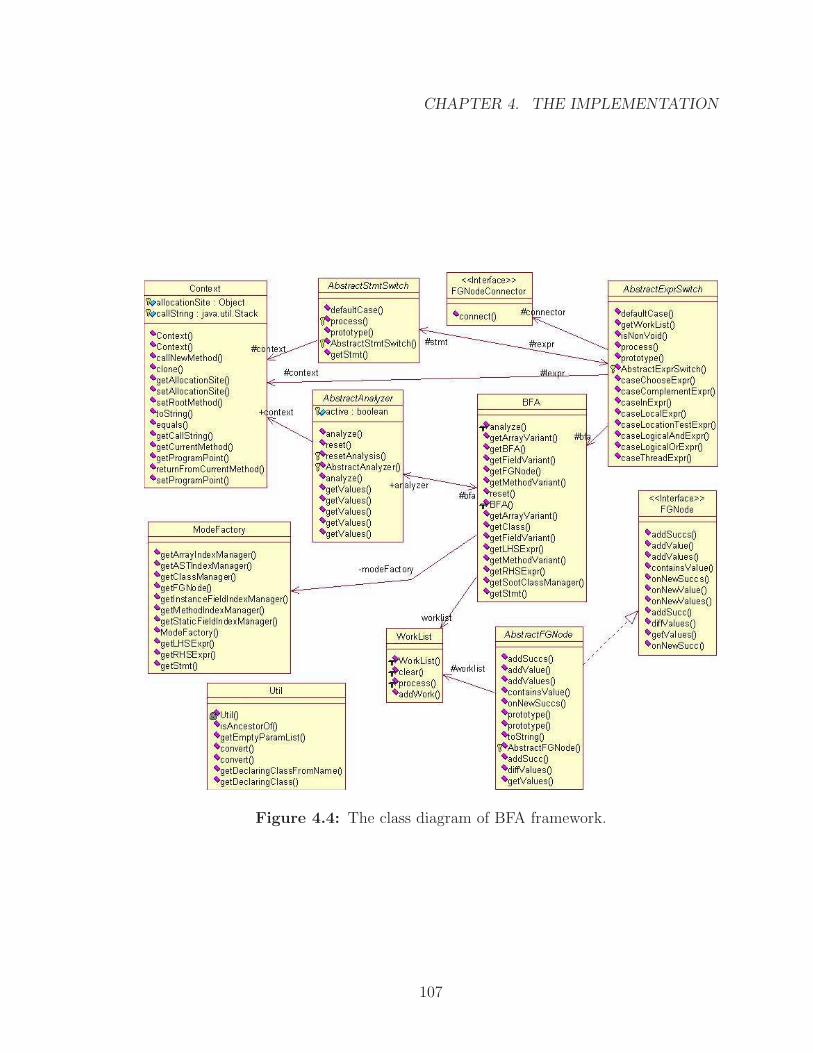
CHAPTER 4. THE IMPLEMENTATION
Figure 4.4: The class diagram of BFA framework.
107
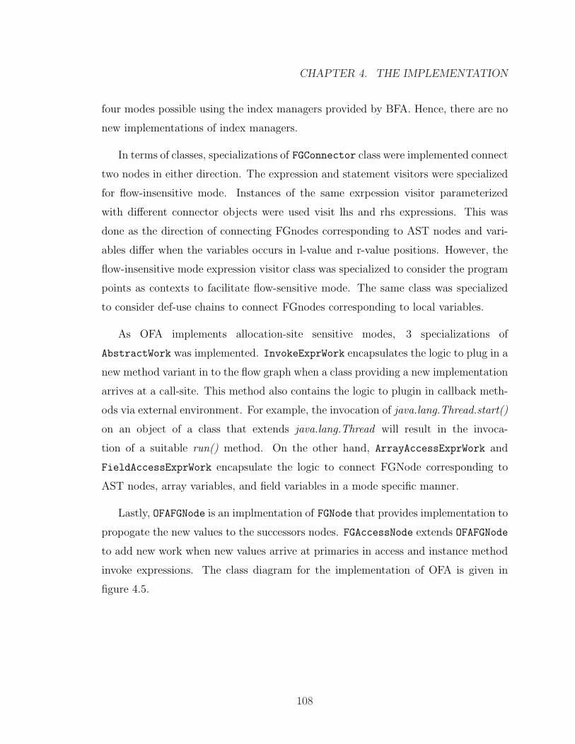
CHAPTER 4. THE IMPLEMENTATION
four modes possible using the index managers provided by BFA. Hence, there are no
new implementations of index managers.
In terms of classes, specializations of FGConnector class were implemented connect
two nodes in either direction. The expression and statement visitors were specialized
for flow-insensitive mode. Instances of the same exrpession visitor parameterized
with different connector objects were used visit lhs and rhs expressions. This was
done as the direction of connecting FGnodes corresponding to AST nodes and vari-
ables differ when the variables occurs in l-value and r-value positions. However, the
flow-insensitive mode expression visitor class was specialized to consider the program
points as contexts to facilitate flow-sensitive mode. The same class was specialized
to consider def-use chains to connect FGnodes corresponding to local variables.
As OFA implements allocation-site sensitive modes, 3 specializations of
AbstractWork was implemented. InvokeExprWork encapsulates the logic to plug in a
new method variant in to the flow graph when a class providing a new implementation
arrives at a call-site. This method also contains the logic to plugin in callback meth-
ods via external environment. For example, the invocation of java.lang.Thread.start()
on an object of a class that extends java.lang.Thread will result in the invoca-
tion of a suitable run() method. On the other hand, ArrayAccessExprWork and
FieldAccessExprWork encapsulate the logic to connect FGNode corresponding to
AST nodes, array variables, and field variables in a mode specific manner.
Lastly, OFAFGNode is an implmentation of FGNode that provides implementation to
propogate the new values to the successors nodes. FGAccessNode extends OFAFGNode
to add new work when new values arrive at primaries in access and instance method
invoke expressions. The class diagram for the implementation of OFA is given in
figure 4.5.
108
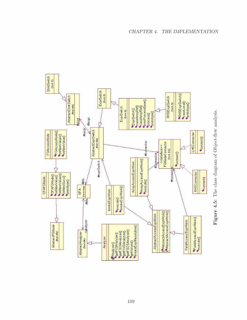
CHAPTER 4. THE IMPLEMENTATION
Fig
ure
4.5
:T
he
clas
sdia
gram
ofO
bje
ct-fl
owan
alysi
s.
109
Chapter 5
Application
This chapter cites real world examples where BOFA is (can) being used with suitable
illustrations.
5.1 Program Slicing
Program Slicing1 can be improved substantially with inter-procedural data-flow infor-
mation pertaining to the Java program. In simple words, Program Slicing is technique
in which a given chunk of code, S, is transformed into another chunk of code, Sc, by
“slicing” away parts of the S.
Speaking more technically, a chunk of code S which needs to be transformed, and
a criteria c which guides or controls the “slicing” are the inputs to program slicing.
c is usually a program point in S and is called as the slicing criterion. The aim of
program slicing is to remove part of code from S which do not influence the result
of evaluating c. This means that the result of executing c both in S and Sc will be
identical. If the slicing criteria is chosen wisely, then Sc will be a shorter chunk of
code compared to S. In this case, if the same model extraction technique is used to
1[HCD+99] provides a gentle introduction to slicing of Java software. For more rigorous treate-ment of slicing of Java software in accordance with model checking, please refer to [DH99].
110
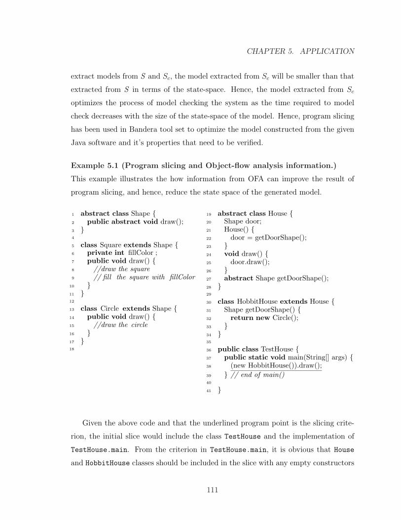
CHAPTER 5. APPLICATION
extract models from S and Sc, the model extracted from Sc will be smaller than that
extracted from S in terms of the state-space. Hence, the model extracted from Sc
optimizes the process of model checking the system as the time required to model
check decreases with the size of the state-space of the model. Hence, program slicing
has been used in Bandera tool set to optimize the model constructed from the given
Java software and it’s properties that need to be verified.
Example 5.1 (Program slicing and Object-flow analysis information.)
This example illustrates the how information from OFA can improve the result of
program slicing, and hence, reduce the state space of the generated model.
1 abstract class Shape {2 public abstract void draw();3 }4
5 class Square extends Shape {6 private int fillColor ;7 public void draw() {8 //draw the square9 // fill the square with fillColor
10 }11 }12
13 class Circle extends Shape {14 public void draw() {15 //draw the circle16 }17 }18
19 abstract class House {20 Shape door;21 House() {22 door = getDoorShape();23 }24 void draw() {25 door.draw();26 }27 abstract Shape getDoorShape();28 }29
30 class HobbitHouse extends House {31 Shape getDoorShape() {32 return new Circle();33 }34 }35
36 public class TestHouse {37 public static void main(String[] args) {38 (new HobbitHouse()).draw();39 } // end of main()40
41 }
Given the above code and that the underlined program point is the slicing crite-
rion, the initial slice would include the class TestHouse and the implementation of
TestHouse.main. From the criterion in TestHouse.main, it is obvious that House
and HobbitHouse classes should be included in the slice with any empty constructors
111
CHAPTER 5. APPLICATION
defined in them as an instance of HobbitHouse is being created using a default con-
structor at line 38. The default construtor of HobbitHouse will invoke the default
constructor of House, and hence, House.House() will be included in the slice. As a
result of this, Shape class is included in the slice as House class has a member variable,
door, of the type Shape. Also, as getDoorShape is invoked at line 22, and there is no
implementation for it in House, getDoorShape implementation in all the subclasses
of House included in the slice also need to be included in the slice. From the slicing
criterion, it is also obvious that House.draw will be invoked, as HobbitHouse does
not provide an implementation of draw method. Hence, HobbitHouse.draw will also
be included in the slice.
This is the point where things get a bit fuzzy due to lack of run-time information
at the time of static analysis. The static type of door is Shape. This means door
can refer to objects of any subclass of Shape, and hence, the implementation of draw
method as provided by the subclasses will be invoked at line 25.
By mere class hierarchy analysis, this would suggest both Circle and Square to
be included in their entirety. However, by inspecting the given chunk of code, it is
clear that the implementation of draw provided by Circle class will be executed at
line 25. The results from OFA can be used to arrive at this conclusion as the summary
set for this variable at line 25 will contain object of type Circle.
The impact of the exclusion of unnecessary data from the model as done in this
example is dependent on the type of data that is sliced away and the type of model
checking being used. Square.fillColor is an integer variable, and hence, it is hard
to statically determine it’s run-time value. Usually, such variables are abstracted as
bounded variables. Even in such cases, naively, the state space of the extracted model
can increase by folds equal to the number of values in the bound of the variable. For
example, if we assume that there can be 255 colors, the size of the state space when
the draw method in Square is included will be approximately 255 times larger than
that when it is not included.
112
CHAPTER 5. APPLICATION
In cases, where variables are unbounded and the domain of their values is large,
the amount of reduction in the state space of the extracted model due to slicing of
unnecessary parts of the program would be drastic when the variables are considered
during model checking.
End of Example
5.2 Method Inlining
Model checkers are simple. They are usually made up of data, logic, and simple
constructs sufficient to program models and verify their properties. They do not
support fancy stuff such as methods, objects, etc. In such a case, generating a model
of software written in a feature rich language such as Java calls for techniques to
realize it’s rich features in the language acceptable by the model checker. Method
Inlining can be thought of as one such technique to realize method calls in Java in
model checker languages such as Promela which do not support functions.
Method Inlining is a program transformation technique in which the body of the
method is inlined at the method call-site. Apart from the complexity involved in
satisfying various semantic specifications of the language during inlining, features
such as dynamic dispatch add another level of complexity. Dynamic dispatch defers
the decision of which method implementation to invoke at a call-site to run-time.
Hence, to perform inlining at a dynamic dispatch call-site, one needs to approximate
the method implementations that shall be invoked at run-time at the given call-site,
and inline a conditional statements to execute method implementations corresponding
to the values arriving at the receiver at run-time.
Example 5.2 (Method inlining and Object-flow analysis information.)
This example illustrates how method inlining is realized during model construction
in languages that do not support functions/methods, and how OFA information can
contribute to the situation.
113
CHAPTER 5. APPLICATION
Consider the source code given in example 5.1. If method inlining were to be
done in the model constructed to represent the given source code, the issue would
be at line 22 and line 25 as the call-sites involve dynamic dispatch. In the former
case, it is trivial in the given source code as only on implementation of draw exists
and it is reasonable to inline it’s body. However, in the latter case, there are two
implementations. The usually way to inline in such situation is to inline a conditional
with the body of the possible method implementations serving as the body of each
branch of the conditional. In case of the example, a conditional would check the
type of the receiver at run-time, if it is of type Square then the branch in which the
implementation of Square.draw is inlined is executed. If it is of type Circle, the
branch in which the implementation of Circle.draw is inlined is executed.
As in the case of slicing, it would be a waste of space and time as it can be deter-
mined via OFA that Circle.draw will be executed at line 25. Hence, the conditional
can be replaced by the body of Circle.draw.
End of Example
Although the optimizations possible in inlining and slicing seem trivial, the re-
duction in the state space of the model achieved by removing unnecessary parts of
the system bears a great impact on the performance of model checking.
5.3 Trivial Optimizations
There are two trivial optimizations that can use information from OFA.
The first one being a check if a reference can evaluate to null at run-time. This is
accomplished via a rather conservative data-flow analysis in javac. OFA can provide
the same information for class variables, instance variables, and array components.
According to [GJS00], “Each class variable, instance variable, or array component is
initialized with a default value when it is created.” This should occur in <clinit>
114
CHAPTER 5. APPLICATION
method, <init> method, and the array creation expressions, respectively. A simple
way to calculate such information would be check if the class variables and instance
variables have empty summary sets at the end of <clinit> and <init> methods,
respectively. If so, then it is possible that such variables can evaluate to null. This
is a rather conservative approach.
The second optimization being that the dynamic type information can be used
in conjunction with instanceof expression to statically determine if the expression
will evaluate to true or false. If it is statically determined that the expression will
evaluate to false, the body of the condition can be transformed suitably to reduce
space and improve speed. This is useful in optimizing instances of frameworks.
115
Chapter 6
Future Work
This chapter concludes the thesis by highlighting the current limitaions and proposing
new ideas to extend BFA.
6.1 Current Limitations
There are two main limitations in BFA that prevent it from being used in more
aggressive manner.
BFA does not handle concurrency. In terms of concepts presented in earlier chap-
ters, the current implementation of BFA does not provide to perform thread-sensitive
flow analysis. This is due to the fact that number of interleavings possible during
run-time is high depending on how the multi-threaded programs are sructured, and
hence, will lead to huge amount of run-time memory requirements. A more important
reason for this limitation is the need for such precise analysis is not obvious at this
time. Although this reason seems lame, it is pointless to implement an analysis which
has no practical use. However, it would be interesting to investigate if maintaining
flow-sensitive information for fields inside synchronized blocks improve the precision
of the analysis.
116
CHAPTER 6. FUTURE WORK
Another limitation is that BFA supports allocation-site sensitive flow information,
but not object sensitive flow information. Although object sensitive flow information
would be more precise, it is hard to differentiate various instances created by the
same allocation site. An allocation site embedded in the body of a loop gives rise
to one such situation. It may be the case that attributes of objects created by this
allocation site indeed have different values at run-time, but this is not perceived
during flow analysis as it is hard to calculate the number of objects created in a loop.
We present a plausible solution to this situation in the next section.
Apart from these two limitations in terms of features, there are a few more in terms
of syntactic and semantic language features that are not addressed in the current
implementation of OFA. The first such limitations arises from the exception handling
support available in Java. In Java, an exception thrown at a location can be caught in
any of the enclosing scope. In terms of language semantics, the variable in the catch
statement will refer to the exception object caught. In simple terms, the thrown
exception object is assigned to the parameter of the catch clause of the try-catch
statement which catches the exception. Although this is an assignment, it is not
a trivial assignment as the lhs and rhs expressions can occur in different scopes.
This problem can be remedied by maintaining a flow graph nodes that summarize
exceptions for a block of statements in a method and these nodes need to be connected
to the flow graph nodes corresponding to the plausible catch clause parameter. Soot
has some support in terms of CompleteStmtGraph and SimpleLocalDefs to retrieve
information regarding local throw catches in the form of def-use chains. This can be
a possible extension to the existing implementation of OFA.
The second limitation arises from the threading model in Java. In Java, threading
can be achieved in two ways. One is by a class, MyThread, extending
java.lang.Thread1 and implementing java.lang.Thread.run(). A thread is cre-
ated when an object of type MyThread is created, and the thread is executed when
start() (this should be the method as implemented in Thread) is invoked on this
1In the future, we shall use Thread to refer to java.lang.Thread.
117
CHAPTER 6. FUTURE WORK
object. The other way is for a class, MyRun, to implement java.lang.Runnable
interface and implement java.lang.Runnable.run(). A thread is now created by
creating a Thread object and passing an instance of MyRun as an argument to it’s con-
structor. However, the thread is executed by calling start() on the Thread object.
This will in turn invoke the MyRun.run() method. This mechanism is internal to the
implementation of Thread. There is no limitation in the first case, as the correspond-
ing run() method can be processed when a start() method is encountered as both
these methods will be defined in the same class hierarchy branch. In the second case,
the start() and run() implementations can occur in different branches of the class
hierarchy. Hence, to process the corresponding run() method the object provided
as the argument to the constructor of Thread should be known. This means the
implementation of Thread should be available during the analysis. This brings us to
the limitation that the system needs to be closed to provide precise results. However,
it is possible in certain cases to close the system via approximate specification from
the user. We defer the idea of how to achieve this to the next.
The next limitation stems from the previous one. What if the system is not
closed and one cannot specify properties about the external environment? The two
alternative would be: the analysis cannot proceed unless the system is closed, or
perform the modular analysis. The second option is interesting as it does not throw
in the towel. In simple words, the second option means that it should be possible to
analyze fragments of the system and combine this information at a later time. This
also means that it should be possible to stage the analysis in phases. Although it is
an enticing option, it is a hard one too. The reason being that information calculated
by the analysis for a fragment of the system should be serializable. This requires
a format or a syntax to represent the information from the analysis. Also, given
the fragment of the system, it should be possible to quickly verify if the serialized
information indeed corresponds to the given fragment of the system. This is similar
to class versioning. One wouldn’t want to use the analysis information pertaining to a
different implementation of the system fragment even though the interface is identical.
Although the problem seems hard, it is a worhty research problem to modularize flow
118
CHAPTER 6. FUTURE WORK
analysis in a simple and efficient manner.
6.2 Possible Extensions
The following are suggestions or ideas (probably somebody’s nightmare) to extend
BFA.
• Currently, BFA provides support for flow and allocation-site sensitive modes of
analysis. However, it has infrasturcture to enable call-stack sensitive mode of
analysis. This would be referred to as k-CFA in traditional literature. It would
be an interesting to complete this infrastructure to enable call-stack sensitive
mode of analysis.
• Given the observation in example 3.3, it is an interesting problem to explore
the possibilities of staging OFA or any static analyses in phases. The question
to be answered will be “Can static analyses such as OFA can be staged?”. In
stage one of the analysis the relation between various entities in a procedure
is calculated in terms of symbolic values. This information is later on used by
binding concrete values to the symbolic values and combining the information
from various procedures to obtain information of required precision and locality.
This would be similar to offline partial evaluation and incremental compilation.
On the surface, it seems there would be considerable reduction in run-time
storage and improvement in speed.
• As mentioned in the previous section, it is hard to differentiate various instances
of objects created by an allocation-site. However, information regarding flow of
objects through the primary in def and use sites can alleviate this issue. If an
oracle can assure that the primary at the def site of a field will evaluate to the
same object at the use site of the field, then this information can help add some
flow-sensitivity into the flow information concerned with fields and arrays. Such
oracle can represent the objects as symbols and these symbols can be unified
119
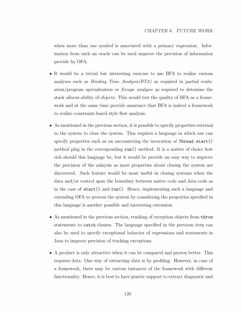
CHAPTER 6. FUTURE WORK
when more than one symbol is associated with a primary expression. Infor-
mation from such an oracle can be used improve the precision of information
provide by OFA.
• It would be a trivial but interesting exercise to use BFA to realize various
analyses such as Binding Time Analysis(BTA) as required in partial evalu-
ation/program specialization or Escape analysis as required to detemine the
stack allocat-ability of objects. This would test the quality of BFA as a frame-
work and at the same time provide assurance that BFA is indeed a framework
to realize constraint-based style flow analysis.
• As mentioned in the previous section, it is possible to specify properties external
to the system to close the system. This requires a language in which one can
specify properties such as on encountering the invocation of Thread.start()
method plug in the corresponding run() method. It is a matter of choice how
rich should this language be, but it would be provide an easy way to improve
the precision of the anlaysis as more properties about closing the system are
discovered. Such feature would be most useful in closing systems when the
data and/or control span the boundary between native code and Java code as
in the case of start() and run(). Hence, implementing such a language and
extending OFA to process the system by considering the properties specified in
this language is another possible and interesting extension.
• As mentioned in the previous section, tracking of exception objects from throw
statements to catch clauses. The language specified in the previous item can
also be used to specify exceptional behavior of expressions and statements in
Java to improve precision of tracking exceptions.
• A product is only attractive when it can be compared and proven better. This
requires data. One way of extracting data is by profiling. However, in case of
a framework, there may be various instances of the framework with different
functionality. Hence, it is best to have generic support to extract diagnostic and
120
CHAPTER 6. FUTURE WORK
statistical information about an instance of a framework. In particular, extract
such information over numerous execution. For example, a common question
in flow analysis is “how many summary sets will the analysis create for a given
input?” This question can be easily answered if such daignostic support is
available in BFA. It would be an interesting task to design and implement such
support in BFA.
• The idea of modularizing flow analysis and later on combining these to generate
more useful information is a possible extension to this framework, although it
must be said that modular and compositional flow analysis is a research topic
in itself.
121
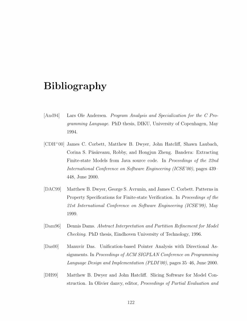
Bibliography
[And94] Lars Ole Andersen. Program Analysis and Specialization for the C Pro-
gramming Language. PhD thesis, DIKU, University of Copenhagen, May
1994.
[CDH+00] James C. Corbett, Matthew B. Dwyer, John Hatcliff, Shawn Laubach,
Corina S. Pasareanu, Robby, and Hongjun Zheng. Bandera: Extracting
Finite-state Models from Java source code. In Proceedings of the 22nd
International Conference on Software Engineering (ICSE’00), pages 439–
448, June 2000.
[DAC99] Matthew B. Dwyer, George S. Avrunin, and James C. Corbett. Patterns in
Property Specifications for Finite-state Verification. In Proceedings of the
21st International Conference on Software Engineering (ICSE’99), May
1999.
[Dam96] Dennis Dams. Abstract Interpretation and Partition Refinement for Model
Checking. PhD thesis, Eindhoven University of Technology, 1996.
[Das00] Manuvir Das. Unification-based Pointer Analysis with Directional As-
signments. In Proceedings of ACM SIGPLAN Conference on Programming
Language Design and Implementation (PLDI’00), pages 35–46, June 2000.
[DH99] Matthew B. Dwyer and John Hatcliff. Slicing Software for Model Con-
struction. In Olivier danvy, editor, Proceedings of Partial Evaluation and
122
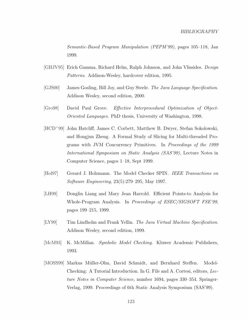
BIBLIOGRAPHY
Semantic-Based Program Manipulation (PEPM’99), pages 105–118, Jan
1999.
[GHJV95] Erich Gamma, Richard Helm, Ralph Johnson, and John Vlissides. Design
Patterns. Addison-Wesley, hardcover edition, 1995.
[GJS00] James Gosling, Bill Joy, and Guy Steele. The Java Language Specification.
Addison Wesley, second edition, 2000.
[Gro98] David Paul Grove. Effective Interprocedural Optimization of Object-
Oriented Languages. PhD thesis, University of Washington, 1998.
[HCD+99] John Hatcliff, James C. Corbett, Matthew B. Dwyer, Stefan Sokolowski,
and Hongjun Zheng. A Formal Study of Slicing for Multi-threaded Pro-
grams with JVM Concurrency Primitives. In Proceedings of the 1999
International Symposium on Static Analysis (SAS’99), Lecture Notes in
Computer Science, pages 1–18, Sept 1999.
[Hol97] Gerard J. Holzmann. The Model Checker SPIN. IEEE Transactions on
Software Engineering, 23(5):279–295, May 1997.
[LH99] Donglin Liang and Mary Jean Harrold. Efficient Points-to Analysis for
Whole-Program Analysis. In Proceedings of ESEC/SIGSOFT FSE’99,
pages 199–215, 1999.
[LY99] Tim Lindholm and Frank Yellin. The Java Virtual Machine Specification.
Addison Wesley, second edition, 1999.
[McM93] K. McMillan. Symbolic Model Checking. Kluwer Academic Publishers,
1993.
[MOSS99] Markus Muller-Olm, David Schmidt, and Bernhard Steffen. Model-
Checking: A Tutorial Introduction. In G. File and A. Cortesi, editors, Lec-
ture Notes in Computer Science, number 1694, pages 330–354. Springer-
Verlag, 1999. Proceedings of 6th Static Analysis Symposium (SAS’99).
123
BIBLIOGRAPHY
[Muc97] Steven S. Muchnick. Advanced Compiler Design & Implementation. Mor-
gan Kaufmann Publishers. Inc., San Francisco, California, USA, 1997.
[NNH99] Flemming Nielson, Hanne Riis Nielson, and Chris Hankin. Principles of
Program Analysis. Springer, 1999.
[Ste96] Bjarne Steensgaard. Points-to Analysis in Almost Linear Time. In Con-
ference Record of the 23th Annual ACM Symposium on Principles of Pro-
gramming Languages(POPL’96), pages 32–41. ACM Press, Jan 1996.
[VR00] Raja Vallee-Rai. SOOT: A Java Bytecode Optimization Framework. Mas-
ter’s thesis, School of Computer Science, McGill University, Oct 2000.
124


![[XLS] · Web viewPuliveerthi Vineela A Meena Chowdary Syed Mohammed Peershavali K S Gunashekar D Sandhya Sri Gunta Upendra R Ranganath Reddy Siva Prasad V Mythri E C Samba Siva Reddy](https://img.pdfslide.us/doc/110x75/5ae9d4f17f8b9a0877917579/xls-viewpuliveerthi-vineela-a-meena-chowdary-syed-mohammed-peershavali-k-s-gunashekar.jpg)