Embed Size (px)
Citation preview

1
Numerical Methods
Process Systems Engineering
ITERATIVE METHODS
Numerical methods in chemical
engineering
Edwin Zondervan

2
Numerical Methods
Process Systems Engineering
OVERVIEW
• Iterative methods for large systems of
equations
• We will solve Laplace’s equation for
steady state heat conduction

3
Numerical Methods
Process Systems Engineering
LAPLACE’S EQUATIONS
Tt
T 2
Thermal diffusivity
The steady state problem:
0
0
2
2
2
2
2
y
T
x
T
T
x
y
T=Tb1
T=Tb2
T=Tb4T=Tb3
(4-1)
(4-2)
(4-3)

4
Numerical Methods
Process Systems Engineering
TRACK TEMPERATURE ON A
GRID
i =1 i =2 i =3
j =1
j =2
j =3
T1 T2 T3
TNx+1 TNx+2 TNx+3
i =Nx
j =Ny
…
…
TNx
T2Nx
(Ny-1)Nx+1
Index of a node is
given by:
K = i + Nx(j-1)
So that:
Ti,j = Tk=i+Nx(j-1)

5
Numerical Methods
Process Systems Engineering
ESTIMATES OF THE SECOND
DIFFERENTIALS FOR x• Assume a piece-wise linear profile in the
temperature, e.g.:
Ti+1
Ti
Ti-1
x x
x
T
x
x
T
x
T
x
T ii 2/12/1
2
2
2
,1,,1
,1,,,1
2
x
TTT
x
x
TT
x
TT
jijiji
jijijiji
(4-4)
(4-5)

6
Numerical Methods
Process Systems Engineering
INCLUDE THE ESTIMATES OF THE
SECOND DIFFERENTIALS FOR y
022
2
,1,,1
2
,1,,1
y
TTT
x
TTT jijijijijiji
Equal spaced grid x = y =1
04 11 NxkkkkNxk TTTTT
(4-6)
(4-7)
(4-8)
022
22
11
y
TTT
x
TTT NxkkNxkkkk

7
Numerical Methods
Process Systems Engineering
BOUNDARY CONDITIONS
• For the nodes on the boundary, we have a
simple equations:
• The equation on the previous slide and the
boundaries can be written as a matrix
equation:
temperaturefixedsome,boundarykT
bAT
(4-9)
(4-10)

8
Numerical Methods
Process Systems Engineering
LET’S WRITE THIS STUFF AS
MATRIX EQUATIONS
Nx=5; %number of points along x direction
Ny=5; %number of points in the y direction
d = 1/Nx; %the grid spacing
Alpha = 1; %thermal diffusivity
e = ones(Nx*Ny,1);
A = spdiags([e,e,-4*e,e,e],[-Nx,-1,0,1,Nx],Nx*Ny,Nx*Ny);
A = A*alpha/d^2;

9
Numerical Methods
Process Systems Engineering
MATRIX SPARSITY
Spy(A) Nx=Ny = 5
A sparse matrix structure,
which is not tridiagonal: there
are offset bands.
Offset bands can cause
your trouble!!
0 5 10 15 20 25
0
5
10
15
20
25
nz = 113
10
Numerical Methods
Process Systems Engineering
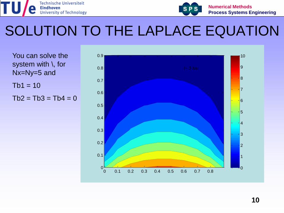
SOLUTION TO THE LAPLACE EQUATION
You can solve the
system with \, for
Nx=Ny=5 and
Tb1 = 10
Tb2 = Tb3 = Tb4 = 0
t= 3 tau
0 0.1 0.2 0.3 0.4 0.5 0.6 0.7 0.80
0.1
0.2
0.3
0.4
0.5
0.6
0.7
0.8
0.9
0
1
2
3
4
5
6
7
8
9
10
11
Numerical Methods
Process Systems Engineering
LU decomposition
0 10 20
0
5
10
15
20
25
nz = 129
0 10 20
0
5
10
15
20
25
nz = 129
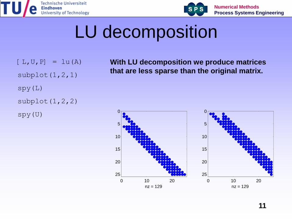
[L,U,P] = lu(A)
subplot(1,2,1)
spy(L)
subplot(1,2,2)
spy(U)
With LU decomposition we produce matrices
that are less sparse than the original matrix.

12
Numerical Methods
Process Systems Engineering
LU DECOMPOSITION
• Gaussian elimination on a matrix like A
requires more memory (with 3D problems,
the offset in the diagonal would even be
bigger!)
• In general extra memory allocation will not
be a problem for MATLAB
• MATLAB is clever, in that sense that it
attempts to reorder equations, to move
elements closer to the diagonal)

13
Numerical Methods
Process Systems Engineering
ITERATIVE METHODS
• Alternatives for Gaussian elimination
• Use iterative methods when systems are
large and sparse.
• Often such systems are encountered
when we want to solve PDE’s of higher
dimensions (>1D)

14
Numerical Methods
Process Systems Engineering
EXAMPLES
• Jacobi method
• Gauss-Seidel method
• Succesive over relaxation
• bicg – Bi-conjugate gradient method
• gmres – generalized minimum residuals
method
• bicgstab – Bi-conjugate gradient method
15
Numerical Methods
Process Systems Engineering
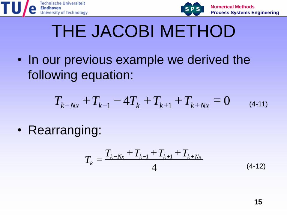
THE JACOBI METHOD
• In our previous example we derived the
following equation:
• Rearranging:
04 11 NxkkkkNxk TTTTT
4
11 NxkkkNxkk
TTTTT
(4-11)
(4-12)

16
Numerical Methods
Process Systems Engineering
THE JACOBI METHOD
• In the Jacobi scheme the iteration
proceeds as follows:
– Start with an initial guess for the values of T at
each node, we calculate an new, updated
values using the equation of the previous
slide and store a new vector:
– Do this for all other nodes, and use new
values as guess, Repeat!
4
,,1,1,
,
oldNxkoldkoldkoldNxk
newk
TTTTT (4-13)
17
Numerical Methods
Process Systems Engineering
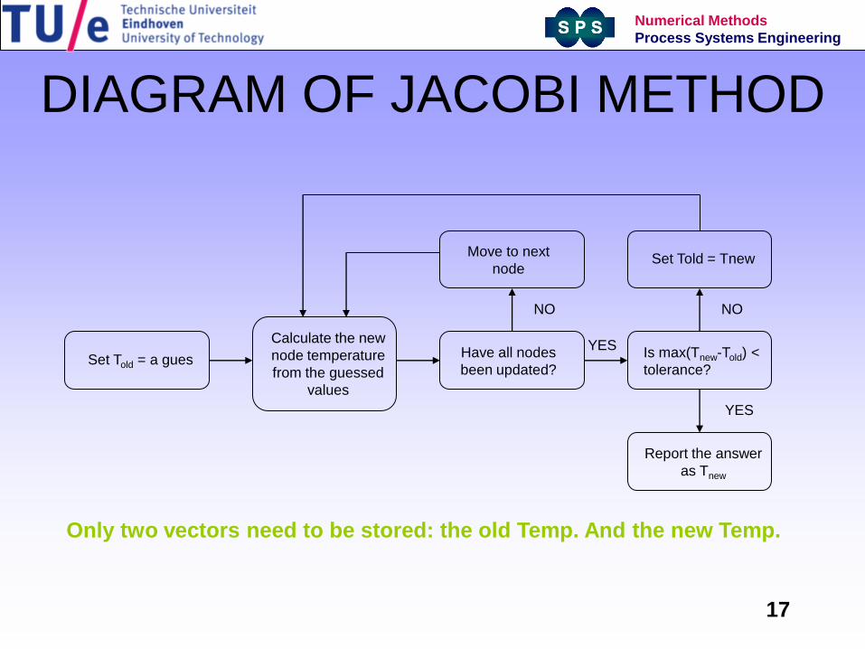
DIAGRAM OF JACOBI METHOD
Set Told = a gues
Calculate the new
node temperature
from the guessed
values
Is max(Tnew-Told) <
tolerance?
Report the answer
as Tnew
Set Told = Tnew
Have all nodes
been updated?
YES
YES
NONO
Only two vectors need to be stored: the old Temp. And the new Temp.
Move to next
node
18
Numerical Methods
Process Systems Engineering
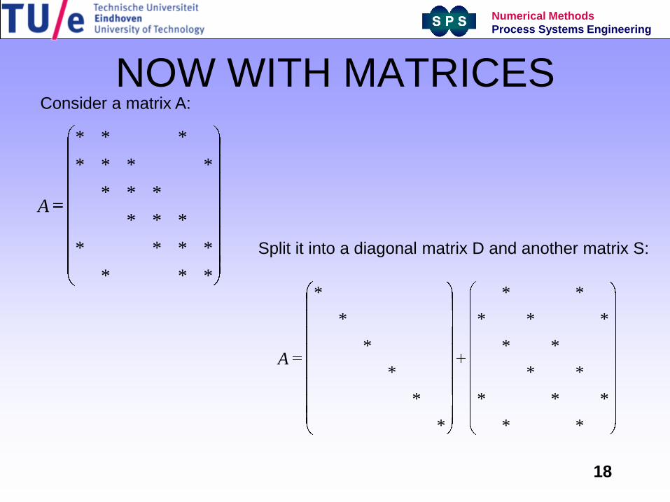
NOW WITH MATRICES
***
****
***
***
****
***
A
**
***
**
**
***
**
*
*
*
*
*
*
A
Consider a matrix A:
Split it into a diagonal matrix D and another matrix S:

19
Numerical Methods
Process Systems Engineering
SOLVE AT-b
• Now we can solve AT=b by:
– (D+S).T = b
– D.T = b –S.T
– D.Tnew = b – S.Told
– Tnew = D-1(b-S.Told)

20
Numerical Methods
Process Systems Engineering
CONVERGENCE OF THE METHOD
• Now we define an error at the k-th iteration:
– errork =Tk - T
• The error at the next iteration is:
– Tk+1 = D-1(b-S.Tk)
– Errork+1 +T = D-1(b-S.errork-S.T)
– D.errork+1=-S.errork
– Errork+1 = -D-1S.errork
Eigenvalues of D-1S must always have modulus < 1, to ensure
that |errork+1| < |errork|
21
Numerical Methods
Process Systems Engineering
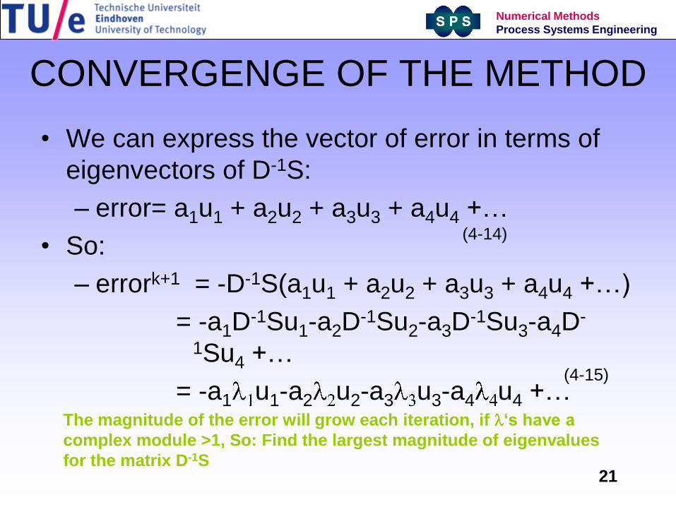
CONVERGENGE OF THE METHOD
• We can express the vector of error in terms of
eigenvectors of D-1S:
– error= a1u1 + a2u2 + a3u3 + a4u4 +…
• So:
– errork+1 = -D-1S(a1u1 + a2u2 + a3u3 + a4u4 +…)
= -a1D-1Su1-a2D
-1Su2-a3D-1Su3-a4D
-
1Su4 +…
= -a1 u1-a2 u2-a3 u3-a4 u4 +…The magnitude of the error will grow each iteration, if ‘s have a
complex module >1, So: Find the largest magnitude of eigenvalues
for the matrix D-1S
(4-14)
(4-15)

22
Numerical Methods
Process Systems Engineering
GERSHGORIN’S THEOREM
• For a square matrix and row k, an eigenvalue is located
on the complex plane within a radius equal or less to the
sum of the moduli of the off-diagonal elements of that
row.
||||||...|||||| ,1,2,2,1,, NkNkNkkkkk mmmmmm
Re( )
Im( )
mk,k
Radius = sum of moduli of
off-diagonal elements
The eigenvalue k must
be in this circle.
(4-16)

23
Numerical Methods
Process Systems Engineering
APPLICATION OF GERSHGORIN’S
THEOREM• Appying Gershgorin’s theorem to our Jacobi
iteration, the off-diagonal elements of row k of D-
1S are 1/ak.k times the off-diagonal elements of
our original matrix A, while the diagonal element
is zero:
• For | k|<1:
kj
kkjk aa |||| ,,
Stability: size of diagonal element must be larger that the sum of moduli of
the other elements, such matrix is called diagonally dominant.
(4-17)

24
Numerical Methods
Process Systems Engineering
SUMMARY
• Partial differential equations can be written as sparse systems of linear equations
• Sparse systems can be handled with a direct method like Gaussian elimination
• If you have systems of more than 1 dimension, a direct method still can be used, if there are no memory issues, otherwise an iterative method may be attractive.
• The Jacobi method was introduced. Many other methods are based on the Jacobi method (SOR method, for example)