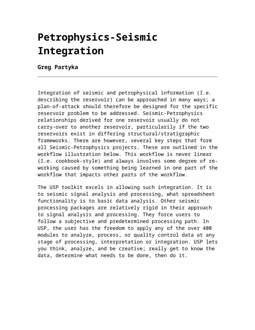
Petrophysics-Seismic IntegrationGreg Partyka

Integration of seismic and petrophysical information (I.e. describing the reservoir) can be approached in many ways; a plan-of-attack should therefore be designed for the specific reservoir problem to be addressed. Seismic-Petrophysics relationships derived for one reservoir usually do not carry-over to another reservoir, particularily if the two reservoirs exist in differing structural/stratigraphic frameworks. There are however, several key steps that form all Seismic-Petrophysics projects. These are outlined in the workflow illustration below. This workflow is never linear (I.e. cookbook-style) and always involves some degree of re-working caused by something being learned in one part of the workflow that impacts other parts of the workflow.

The USP toolkit excels in allowing such integration. It is to seismic signal analysis and processing, what spreadsheet functionality is to basic data analysis. Other seismic processing packages are relatively rigid in their approach to signal analysis and processing. They force users to follow a subjective and predetermined processing path. In USP, the user has the freedom to apply any of the over 400 modules to analyze, process, or quality control data at any stage of processing, interpretation or integration. USP lets you think, analyze, and be creative; really get to know the data, determine what needs to be done, then do it.

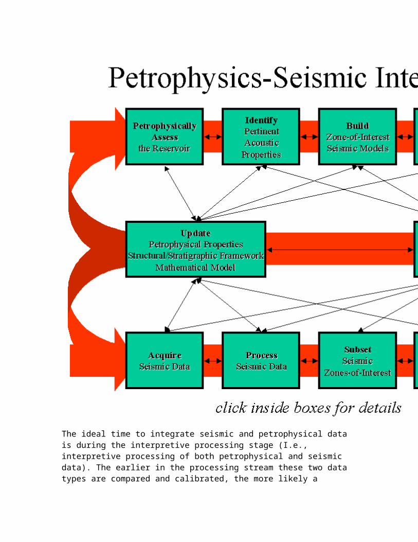
The ideal time to integrate seismic and petrophysical data is during the interpretive processing stage (I.e., interpretive processing of both petrophysical and seismic data). The earlier in the processing stream these two data types are compared and calibrated, the more likely a reasonable reservoir flow-unit characterization will evolve. If integration is pushed down, after completing the petrophysical characterization, and after seismic data is processed and handed off to the interpreter, the integration will become rigid;

dependent on the assumptions built into both the petrophysics and seismic sides of the workflow.

Problems with seismic data processing and petrophysical data processing become most obvious during the integration stage, when mismatches between petrophysical information and geophysical information become evident. If such integration (and problem detection) is done at a late project stage, the interpreter can either force the data together or backup and reprocess the data. In either case, time and quality problem solving is lost.

The petrophysics side of the workflow includes: Petrophysical Assessment of the Reservoir: Using information obtained from boreholes determine the physical and chemical properties of rocks and their fluid content; determining reservoir characteristics such as reservoir thickness, porosity, permeabilty, hydrocarbon saturation, hydrocarbon mobility. Categorize flow-units. Identification of Pertinent Acoustic Properties: Understanding the acoustic manifestation of rock and fluid types via methods such as seismic model, petrophysical-acoustic crossplots, and integration of capillary pressure and acoustic data. Can seismic resolve, or at least detect individual flow units or groups of flow-units? If yes, then 3D seismic should be used to map the spatial and vertical flow-unit boudaries and baffles. Seismic Modeling: Forging an understanding of the acoustic response of the reservoir. This involves building end-member reservoir models from petrophysical rock and fluid types, computing seismic responses for each model, and varying the reservoir thickness/net-to-gross within each model to understand tuning effects. Flow-unit seismic expressions are modeled and understood at this stage. Attribute Extraction from Seismic Reservoir Models: Characterizing reservoir flow-units via attribute components that comprise the seismic waveform; measuring waveform characteristics for each model and identifying discriminating waveform characteristics.

The seismic side of the workflow includes: Seismic Data Acquisition: Optimizing parameters for target depth, target geometry, and surface conditions. Seismic Data Processing: Quality controlling at each step to ensure optimum imaging, Relative amplitude preservation and steep dip preservation. Examine and assess the seismic reservoir map after each processing step to maximize flow-unit imaging. Subsetting the Seismic Zone-of-Interest: Eliminating data areas that will not impact flow-unit interpretation. Attribute Extraction from Processed Seismic Data: Characterizing spatial and vertical flow-unit geometries via attribute components that comprise the seismic waveform.

The common ground between the two sides of the work-flow include: Calibration of Real Seismic Attributes and Modeled Seismic Attributes: Comparing waveform characteristics derived from real seismic data to waveform characteristics derived from modeled seismic data. Similarities strengthen flow-unit calibration; dissimilarities indicate inadequacies in the data, conceptual framework, and/or the mathematical model. Use the insight and knowledge gained in this step along with 3D seismic to map the three-dimensional flow-unit geometries. Re-evaluation of Data, Concepts and Methods: Modeled seismic properties rarely match all aspects of real seismic data. Such discrepancies can be caused by incomplete or inadequate flow-unit characterization, inappropriate structural/stratigraphic framework, or deficient mathematical models.

It is impossible to follow each side of the workflow linearly and independently. Learnings from any of the above steps may impact any or all other step(s).

Return to Online Training

Attribute Extraction from Seismic Reservoir Models

The seismic reflections from reservoir flow-units can be characterized in terms of phase, frequency and amplitude components (i.e. seismic attributes). To facilitate seismic-petrophysics integration, it is important to:

Measure waveform characteristics for each model. Identify waveform characteristics that discriminate and charactrerize flow-units.

The goal of seismic attribute mapping is to quantify flow-units via seismic waveform variability. Steps include:

Spatially Delineate the zone-of-interest, Isolate/Subset the window or boundary that encompass flow-units, Compute seismic attributes within the analysis window,

Reduce attribute measurements to one value per spatial location, Display attribute reductions in map form, Evaluate the spatial geometries/patterns (are they petrophysically significant?), Benchmark the waveform variability to petrophysical/flow-unit properties.

Seismic reflection data can be subdivided into components that make up the seismic waveform:

phase, frequency, amplitude, statics, noise, etc...

Trace attributes such as response phase, energy envelope, spectral decomposition, etc... isolate/subset groups of these seismic waveform characteristics.

Attribute Definitions

USP Attribute GenerationThe modular nature of USP allows thorough and effective signal analysis; whether targeted at model or real seismic data. Programs such as "asig", "spec", etc... in conjunction with "windstat" provide seismic sequence attribute mapping functionality in USP. Signal analysis/attribute results can be view within the USP framework using "xsd".

Return to Seismic-Petrophysics Index.

2D & 3D SEISMIC INTERPRETATION

Generalities

Western AlpsDeep structures

QuaternaryLake Brienz & Rhone Valley

Gulf of Mexico3D sequence stratigraphy

NW Shelf Australia3D structural analysis

Teaching

Consulting

Staff

3D seismic links

 

Section des Sciences de la Terre Université de Lausanne

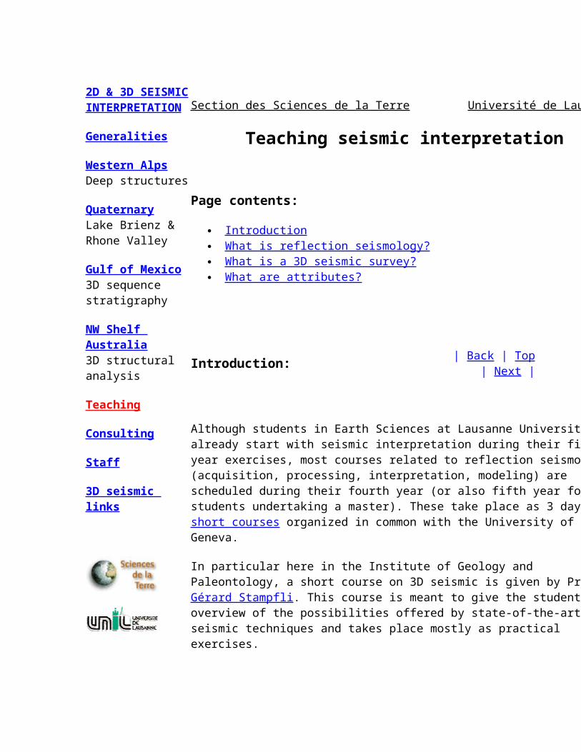
Teaching seismic interpretation 

Page contents:

Introduction What is reflection seismology? What is a 3D seismic survey? What are attributes?

 

Introduction: | Back | Top | Next |

Although students in Earth Sciences at Lausanne University already start with seismic interpretation during their first year exercises, most courses related to reflection seismology (acquisition, processing, interpretation, modeling) are scheduled during their fourth year (or also fifth year for students undertaking a master). These take place as 3 days short coursesorganized in common with the University of Geneva.

In particular here in the Institute of Geology and Paleontology, a short course on 3D seismic is given by Prof. Gérard Stampfli. This course is meant to give the students an overview of the possibilities offered by state-of-the-art 3D seismic techniques and takes place mostly as practical exercises.

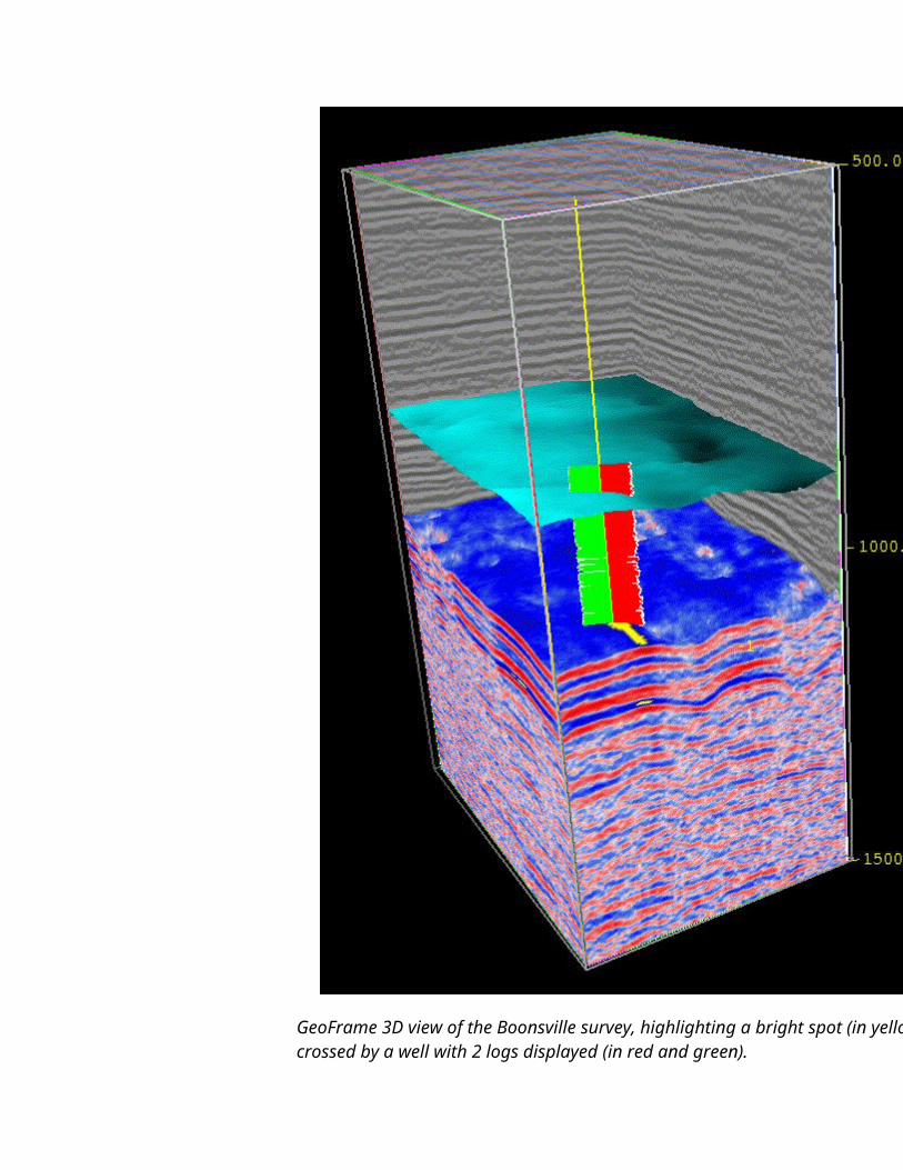
GeoFrame 3D view of the Boonsville survey, highlighting a bright spot (in yellow), crossed by a well with 2 logs displayed (in red and green).

 

For this purpose, we use mainly two small 3D surveys (Stratton and Boonsville) provided by the Bureau of Economic Geology (University of Texas at Austin) as well as the West Cameron survey. These surveys are small and have a large number of wells with logs in digital format and thus offer the students very quick possibilities of mapping and interpreting horizons in a well constrained environment. Furthermore these surveys are quite didactic as they can reveal impressive structural and stratigraphic features. 

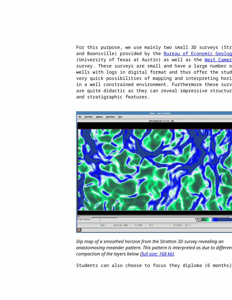
Dip map of a smoothed horizon from the Stratton 3D survey revealing an anastomosing meander pattern. This pattern is interpreted as due to differential compaction of the layers below [full size: 168 kb].

Students can also choose to focus they diploma (6 months) or Masters (18 months) thesis on seismic interpretation.

 

What is reflection seismology? | Back | Top | Next |

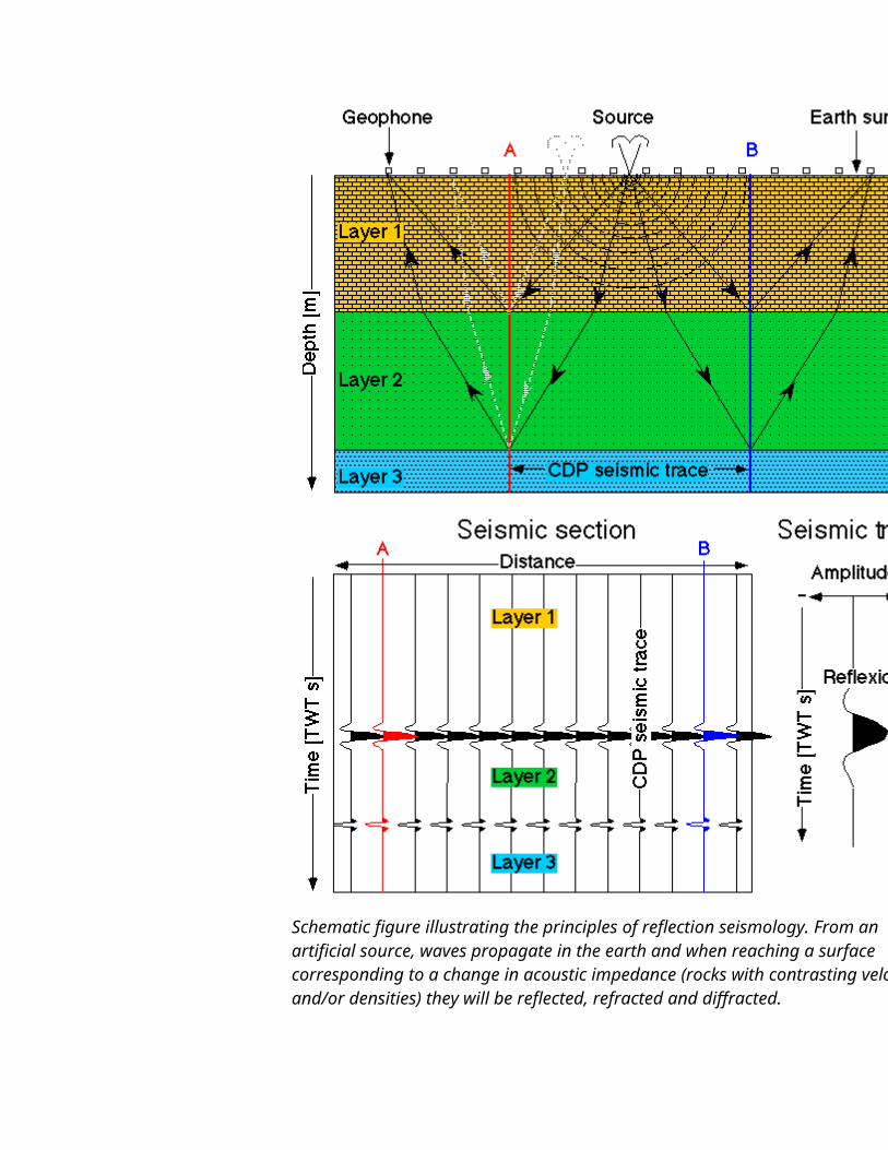
Reflection seismology is the most powerful geophysical method to image the underground and is based on artificial wave sources (explosions, vibrating trucks, etc.). The basic principles are shown below.

Schematic figure illustrating the principles of reflection seismology. From an artificial source, waves propagate in the earth and when reaching a surface corresponding to a change in acoustic impedance (rocks with contrasting velocities and/or densities) they will be reflected, refracted and diffracted.

The travel time of the reflected waves will be recorded by geophones (or hydrophones) as

well as the amplitude of the reflected signal. After a complex processing of the field data, the geologist receives a seismic section (represented here in wiggle display) with a vertical scale corresponding to the two way travel (TWT) time. This seismic section can be compared to a kind of vertical x-ray of the underground which the geologist has to interpret.

 

What is a 3D seismic survey? | Back | Top | Next |

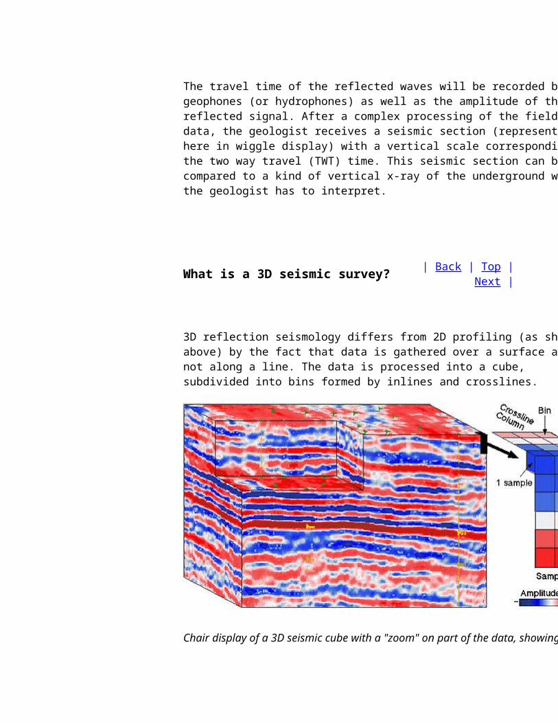
3D reflection seismology differs from 2D profiling (as shown above) by the fact that data is gathered over a surface and not along a line. The data is processed into a cube, subdivided into bins formed by inlines and crosslines.

Chair display of a 3D seismic cube with a "zoom" on part of the data, showing amplitudes samples organized in inlines and crosslines [full size: 105 kb].

Once the 3D survey is loaded on a seismic interpretation workstation, horizons can be automatically mapped and various attribute maps can then be generated. On the basis of this seismic information and of well data, the geologist can obtain a very precise interpretation. This method is now widely used for hydrocarbon production and also exploration.

 

What are attributes? | Back | Top | Next |

Attributes are different ways of looking at the seismic data usually represented in amplitude. They are various mathematical operations done on the seismic data. Depending on the type of input data, the following classes of attributes can be distinguished:

- Property cubes: the whole amplitude cube is transformed (e.g. coherence, termination, etc.).- Seismic attributes: a seismic section is transformed (e.g. reflection strength, apparent polarity, etc.).- Surface attributes: operations done on a surface, usually a mapped horizon (e.g. amplitude, dip & azimuth, etc.).- Volume attributes: operations done on a volume, usually limited by two mapped horizons (e.g. reflection intensity, acoustic impedance, etc.).

These different attributes can help a lot the interpreter as they can highlight various features of the data that would not be visible otherwise.

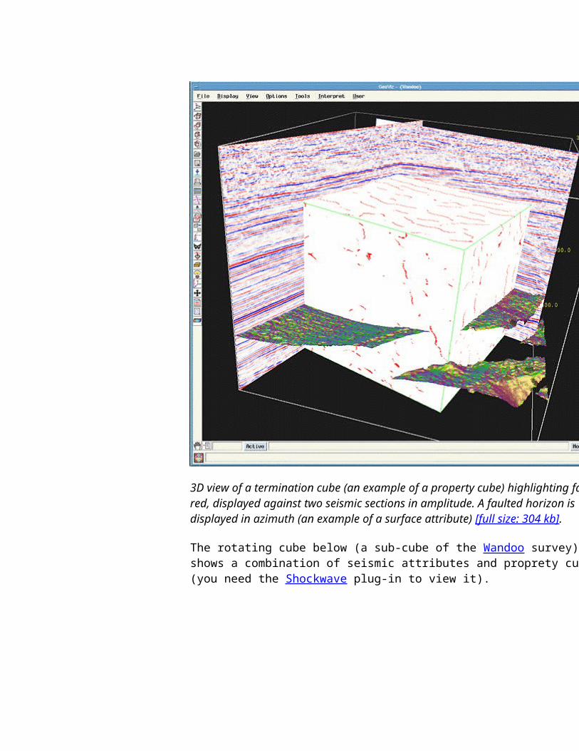
3D view of a termination cube (an example of a property cube) highlighting faults in red, displayed against two seismic sections in amplitude. A faulted horizon is displayed in azimuth (an example of a surface attribute) [full size: 304 kb].

The rotating cube below (a sub-cube of the Wandoo survey) shows a combination of seismic attributes and proprety cube (you need the Shockwave plug-in to view it).

Several examples of the use of attributes for sedimentary environment determination are shown in our case study in the Gulf of Mexico.

Now have a look at our consulting and expertise studies

| Back | Top | Next |

[ Seismic Home ]

| Earth Sciences Home | About us | Research | Search | University of Lausanne |

Last modification: 12-2-2001 By Robin Marchant

 

Reservoir Characterization

   

Indroduction

The characterization of a reservoir includes different aspects, this means we want to describe the geometrical properties as well as the distribution of rock types,  geological facies and petrophysical properties. Since we can' t obtain all this data by direct measurement we have to rely on estimations made on the basis of geostatistical models. They do include all the data available, that is, any measurements made, constraints and possibilities. Modelisation gives us a number of equiprobable solutions which can be used for volumetric computations, quality estimations or optimation of production procedure and help therefore in decision making.

Seismic facies analysis

  Signals on seismic traces are caused by contrast of impedance (density multiplied by seismic velocity) of the ground. Since obvious parameters like the amplitude are closely linked to the impedance ,the same value can be caused by different lithology. So they are not sufficent to discriminate different lithologies. Here seismic facies analysis has been developed.  It is based on the study of seismic attributes. Seismic attributes are parameters which can be calculated using seismic measurements. This parameters include for example phase and frequency of seismic traces, coherence between traces or energy carried by the signal.     They are a great number of attributes which can be used, they have to be choosen in order to be able to distinguish between different lithologies. This choice can be performed using automatic methods : neural nets, statistical methods, automatic classifications, etc. There are two differents approaches in the facies analysis field:

- Supervised segmentation tries to find which operation on the attributes will allow to distinguish best the different facies that have been recognized on well logs. This operation will then be applied on the whole seismic dataset.

- Non supervised segmentation does not take into account facies recognition on well logs. It tries to find out the best way to discriminate several facies or rocktypes given only seismic attributes.

    Although supervised approaches may seem more "seducing" at first look, only comparison with a non supervised approach can show how reliable is the facies distinction it has performed. A good correlation between these two kinds of approach guaranties the geological consistence of the facies distinction.

Lithoseismic interpretation

    The aim of lithoseismic interpretation is to obtain qualitative and quantitative information of the examined ground in addition to structural information. Special interest is given to reservoir properties: the possible content of hydrocarbons, petrophysical properties and the geological facies. With this information we can build a reliable model of the ground.     The principle of lithoseismic interpretation analysis is to find the relation between a seismic attribute and petrophysical properties, fluid properties or rocktypes of the reservoir. Here again, the choice of the good seismic attribute (or combination of seismic attributes) is fundamental.

    As a first step, seismic impedances and other seismic attributes has to be deduced from seismic amplitudes. Then the attributes that bring us the most of information for either facies analysis or reservoir petrophysical and fluids properties have to be pointed out.     A smart way to proceed is to achieve first a seismic facies analysis, in order to discriminate zones of the gound that have a distinct seismic behaviour and to perform a diffrent reservoir properties interpretation on each zone. The obtained properties (porosity, clay volume, fluids saturation, etc.) can then be used for stochastic modeling of the reservoir.

    However, we must keep in mind that the scale of such a lithoseismic interpretation is far more important than the real frequency of variation of the reservoir properties. It should therefore be used as a global trend.

Reservoir simulations

- Data available

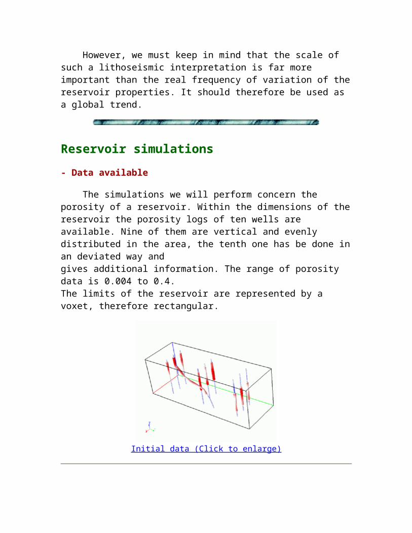
    The simulations we will perform concern the porosity of a reservoir. Within the dimensions of the reservoir the porosity logs of ten wells are available. Nine of them are vertical and evenly distributed in the area, the tenth one has be done in an deviated way and gives additional information. The range of porosity data is 0.004 to 0.4. The limits of the reservoir are represented by a voxet, therefore rectangular.

Initial data (Click to enlarge)

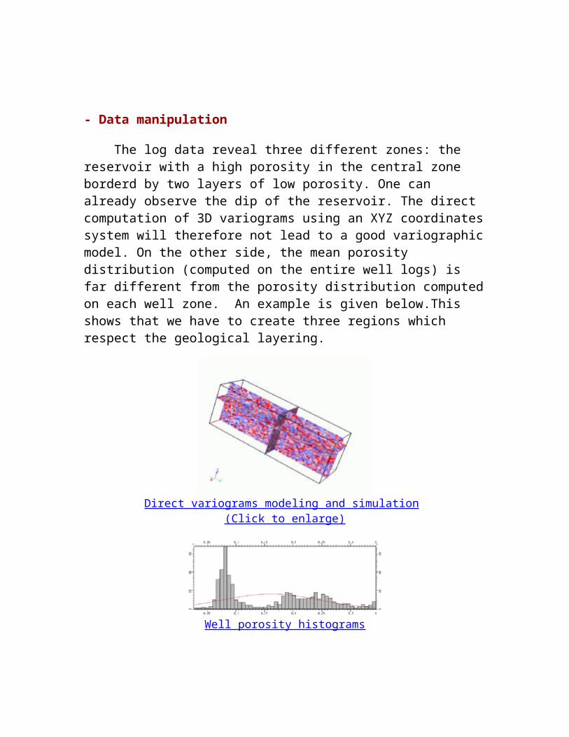
- Data manipulation

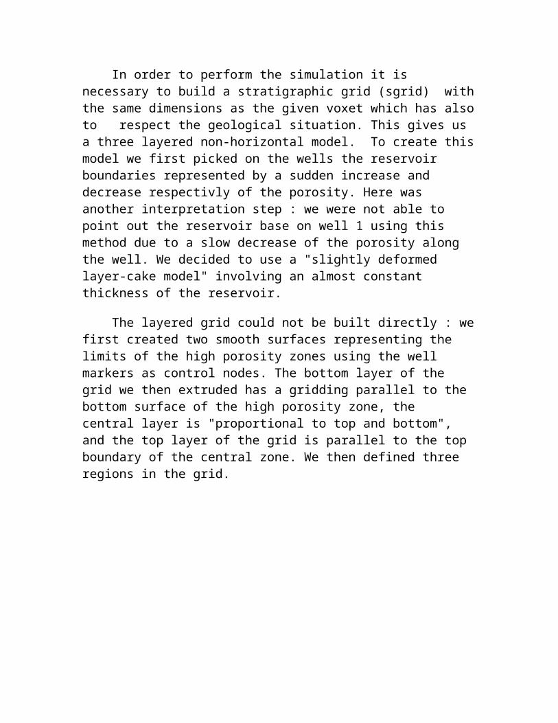
    The log data reveal three different zones: the reservoir with a high porosity in the central zone borderd by two layers of low porosity. One can already observe the dip of the reservoir. The direct computation of 3D variograms using an XYZ coordinates system will therefore not lead to a good variographic model. On the other side, the mean porosity distribution (computed on the entire well logs) is far different from the porosity distribution computed on

each well zone.  An example is given below.This shows that we have to create three regions which respect the geological layering.

Direct variograms modeling and simulation (Click to enlarge)

Well porosity histograms

    In order to perform the simulation it is necessary to build a stratigraphic grid (sgrid)  with the same dimensions as the given voxet which has also to   respect the geological situation. This gives us a three layered non-horizontal model.  To create this model we first picked on the wells the reservoir boundaries represented by a sudden increase and decrease respectivly of the porosity. Here was another interpretation step : we were not able to point out the reservoir base on well 1 using this method due to a slow decrease of the porosity along the well. We decided to use a "slightly deformed layer-cake model" involving an almost constant thickness of the reservoir.

    The layered grid could not be built directly : we first created two smooth surfaces representing the limits of the high porosity zones using the well markers as control nodes. The bottom layer of the grid we then extruded has a gridding parallel to the bottom surface of the high porosity zone, the  central layer is "proportional to top and bottom", and the top layer of the grid is parallel to the top boundary of the central zone. We then defined three regions in the grid.

Surfaces defined from well markers and Voxet borders. (Click to enlarge).

     

Layered SGrid created from the surface model (Click to enlarge)

 

- Simulation and results:

     * Step 1 : Variograms computation and modeling:

   We computed 3D variograms of the well data using an UVW coordinates transformation. Each region was computed separately using conventional variograms. In the reservoir zone we observed very clearly vertical variograms (dip = 85 degree) while horizontal and 45 degree dip did not show such a clear

trend. The variograms also showed an "horizontal" (UV plane) anisotropy : the ranges for the azimuth 0 variograms set were greater than for the others.

    Gaussian models have been used to model reservoir and top zones variograms. Computed models did respect the anisotropy shown on the variograms. The base zone did not show any clear trend, neither horizontaly nor verticaly. We therefore assumed that there was a strong nugget effect in this zone ( that explains half of the variography : nugget effect of 0.5 and seal of 1) and used a spherical model.    

Base layer variograms (click)

Middle layer variograms (click)

Top layer variograms (click)

 

     * Step 2 : Simulations and results:

   After computing the variograms models, we simulated porosity in each region of the SGrid using  a Sequencial Gaussian Simulation. We have choosen this method because we wanted to simulate a continuus property showing a gaussian distribution (by zone, see below), without soft data and taking into account  spatial anisotropies. Five different simulations have been realized. Three different results are shown below.  

Click to load several simulation results

 

Colormap used for   the simulations

Well porosity histograms

 

Grid porosity histogram (central part)

    With this simulated porosity we calculated the porous volume of the reservoir and on the high-porosity zone of the SGrid:

.

Reservoir [volume unit]

High-porosity-zone [volume unit]

Simulation 1 471950 343376

Simulation 2 463103 333943

Simulation 3 481479 344149

Simulation 4 479146 350988

Simulation 5  471701  345655

Total volume  3*10E6 1.47*10E6

Standard deviation 7233  6172

The porous volume is of special interest when regarding a possible exploitation of a reservoir. It gives an information about the amount of oil or gas the reservoir might contain. In our particular case it is a point of view if we consider the entire volume of the reservoir or only the high porosity zone. The differences of the porous volume of the two zones is remarkable and will influence any economic decision making.