Embed Size (px)
Citation preview

1
Numerical Methods
Process Systems Engineering
ORDINARY DIFFERENTIAL
EQUATIONS (ODE’S)
Numerical methods in chemical
engineering
Edwin Zondervan

2
Numerical Methods
Process Systems Engineering
OVERVIEW
• A common problem encountered in engineering is the
initial value problem: how does the state of a system
vary with time, given some starting conditions, when is it
governed by an ODE (Ordinary differential equation)?
• We will look at some simple solvers and numerical
schemes for solving ODE’s
• We will investigate stability so that we are able to choose
a suitable solving method
• In the end we will take a look at systems of coupled
ODE’s

3
Numerical Methods
Process Systems Engineering
EULER’S METHOD
• For the differential equation:
• With the initial condition
• We can generate an estimate of x at t =
t+dt, by a Taylor expansion:
),( txfdt
dx=
0)0( xtx ==
tttxftx
tdt
dxtxttx
d
dd
)),(()(
)()(
+=
+=+
(6-1)
(6-2)
(6-3)

4
Numerical Methods
Process Systems Engineering
MARCHING FORWARD IN
TIME
t t+dt
x(t)
x(t+dt)
The true
solution!
With Euler’s method we can step forward in time …

5
Numerical Methods
Process Systems Engineering
CODE FOR EULER’S METHODfunction[x,t] = Euler(MyFunc,InitialValue,Start,Finish,Nsteps)
x(1) = InitialValue;
t(1) = Start;
dt = (Finish-Start)/Nsteps;
for i =1:Nsteps
F = feval(MyFunc,x(i),t(i));
t(i+1) = dt +t(i);
x(i+1) = F*dt + x(i);
end
t = t’;
x = x’;
return
6
Numerical Methods
Process Systems Engineering
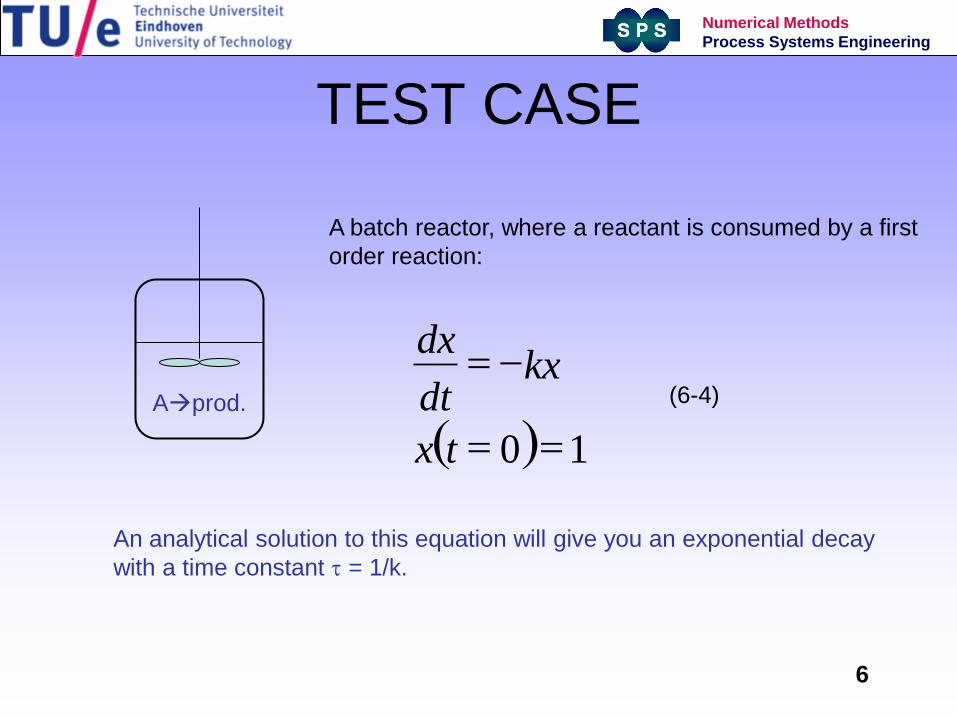
TEST CASE
Aprod.
( ) 10 ==
-=
tx
kxdt
dx
A batch reactor, where a reactant is consumed by a first
order reaction:
An analytical solution to this equation will give you an exponential decay
with a time constant t = 1/k.
(6-4)

7
Numerical Methods
Process Systems Engineering
PERFORMANCE OF EULER’S METHOD
function [f] = TestFunction(x,t)
f = -1*x;
return
For 100 steps, the numerical solution gives a good match!
0 1 2 3 4 5 6 7 8 9 100
0.1
0.2
0.3
0.4
0.5
0.6
0.7
0.8
0.9
1
t
x
Exact
Numerical

8
Numerical Methods
Process Systems Engineering
PERFORMANCE OF EULER’S METHOD
25 STEPS
0 2 4 6 8 10 120
0.1
0.2
0.3
0.4
0.5
0.6
0.7
0.8
0.9
1
t
x
Exact
Numerical
25 Steps: solution OK, small deviation

9
Numerical Methods
Process Systems Engineering
PERFORMANCE OF EULER’S METHOD
6 STEPS:
Oscillates, but tends to
correct asymtpote
0 1 2 3 4 5 6 7 8 9 10-0.8
-0.6
-0.4
-0.2
0
0.2
0.4
0.6
0.8
1
t
xExact
Numerical
6 Steps: solution follows trend, starts
oscillating

10
Numerical Methods
Process Systems Engineering
PERFORMANCE OF EULER’S METHOD
5 STEPS:
Solution becomes
unstable
0 1 2 3 4 5 6 7 8 9 10-1
-0.8
-0.6
-0.4
-0.2
0
0.2
0.4
0.6
0.8
1
t
x
Exact
Numerical
5 Steps: solution becomes unstable
11
Numerical Methods
Process Systems Engineering
PERFORMANCE OF EULER’S METHOD
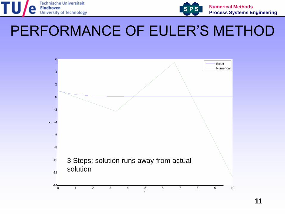
3 STEPS: Solution is
diverging from the true
solution
0 1 2 3 4 5 6 7 8 9 10-14
-12
-10
-8
-6
-4
-2
0
2
4
6
t
x
Exact
Numerical
3 Steps: solution runs away from actual
solution
12
Numerical Methods
Process Systems Engineering
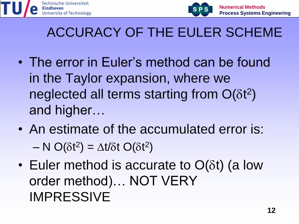
ACCURACY OF THE EULER SCHEME
• The error in Euler’s method can be found
in the Taylor expansion, where we
neglected all terms starting from O(dt2)
and higher…
• An estimate of the accumulated error is:
– N O(dt2) = Dt/dt O(dt2)
• Euler method is accurate to O(dt) (a low
order method)… NOT VERY
IMPRESSIVE

13
Numerical Methods
Process Systems Engineering
STABILITY OF THE EULER
SCHEME• The exact solution to:
lxdt
dx=
And x(t=0) = 1
is: x = exp(lt)For l<0, the solution should decay to zero. Our numerical solution
should do the same…

14
Numerical Methods
Process Systems Engineering
STABILITY OF EULER’S
METHOD
)1(
)()()(1
tx
txx
txftxttx
i
ii
iii
ld
dl
dd
+=
+=
+=++
|(1+ldt)|<1 i.e. -ldt< 2, for the
solution to decay to zero …
So for dt <2 (for l=-1)… Euler is conditionally stable
(6-5)

15
Numerical Methods
Process Systems Engineering
THE IMPLICIT EULER
METHOD• The implicit Euler method uses a gradient
in the future, rather than at a current time
step:
tttxfxx iiidd ),( 11
++=++
(6-5)

16
Numerical Methods
Process Systems Engineering
A SMALL CHANGE IN THE CODEfunction[x,t] = EulerImplicit(MyFunc,InitialValue,Start,Finish,Nsteps)
x(1) = InitialValue;
t(1) = Start;
dt = (Finish-Start)/Nsteps;
for i =1:Nsteps
t(i+1) = dt +t(i);
x(i+1) = fsolve(@FunToSolve,x(i),[],x(i),t(i+1),MyFunc,dt);
end
t = t’;
x = x’;
return
function residual = FunToSolve(x,xo,t,MyFunc,dt)
residual = xo + feval(MyFunc,x,t)*dt-x;
return

17
Numerical Methods
Process Systems Engineering
THE IMPLICIT METHOD
5 STEPS: with the implicit
Euler scheme
0 1 2 3 4 5 6 7 8 9 100
0.1
0.2
0.3
0.4
0.5
0.6
0.7
0.8
0.9
1
t
x
Exact
Numerical

18
Numerical Methods
Process Systems Engineering
STABILITY OF THE IMPLICIT METHOD
)1(
)1(
)()()(
1
1
t
xx
xtx
txx
txftxttx
i1i
i1i
ii
ii1i
ld
ld
dl
dd
+=
=+
+=
+=+
+
+
+
++
lxdt
dx-=The implicit Euler scheme for:
is:
For l<0, the numerical
solution will decay to zero
for any stepsize
(6-6)

19
Numerical Methods
Process Systems Engineering
SYSTEMS OF ODE’S
• We often want to solve coupled ODE’s:
...
),...,,,(
),...,,,(
),...,,,(
3213
3212
3211
txxxfdt
dx
txxxfdt
dx
txxxfdt
dx
=
=
=
(6-7)

20
Numerical Methods
Process Systems Engineering
JUST SMALL CHANGES IN THE EXPLICIT CODE
function[x,t] = EulerCoupled(MyFunc,InitialValue,Start,Finish,Nsteps)
x(:,1) = InitialValue’;
t(1) = Start;
dt = (Finish-Start)/Nsteps;
for i =1:Nsteps
F = feval(MyFunc,x(:,i),t(i));
t(i+1) = dt +t(i);
x(:,i+1) = F*dt + x(:,i);
end
t = t’;
x = x’;
return
Similarly you can adjust the Implicit Euler code
to deal with ODE systems!!!
21
Numerical Methods
Process Systems Engineering
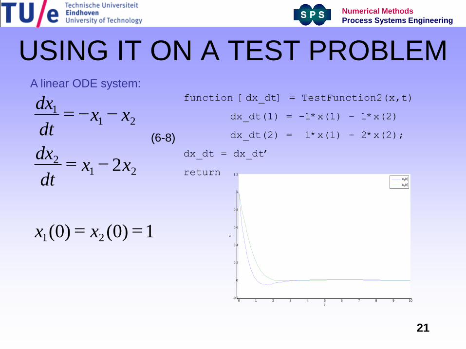
USING IT ON A TEST PROBLEM
1)0()0(
2
21
212
211
==
-=
--=
xx
xxdt
dx
xxdt
dx function [dx_dt] = TestFunction2(x,t)
dx_dt(1) = -1*x(1) – 1*x(2)
dx_dt(2) = 1*x(1) - 2*x(2);
dx_dt = dx_dt’
return
A linear ODE system:
(6-8)
0 1 2 3 4 5 6 7 8 9 10-0.2
0
0.2
0.4
0.6
0.8
1
1.2
t
x
x1(t)
x2(t)

22
Numerical Methods
Process Systems Engineering
STABILITY OF ODE SYSTEMS
• Let’s evaluate our example:
• For linear systems we can get an analytical solution by factorizing M:
• M = U-1LU
-
--=
2
1
2
1
21
11
x
x
x
x
dt
d
M
(6-9)

23
Numerical Methods
Process Systems Engineering
STABILITY OF ODE SYSTEMS
L=
L=
L=
-
-
2
1
2
1
2
11
2
1
2
11
2
1
x
xU
x
xU
dt
d
x
xUUU
x
x
dt
dU
x
xUU
x
x
dt
d
=
L=
=
2
1
2
1
2
1
2
1
2
1
2
1
2
1
0
0
y
y
y
y
dt
d
y
y
y
y
dt
d
x
xU
y
y
l
l
A diagonal matrix: equations are no
longer coupled, and a solution can be
found!!(6-10)
(6-11)

24
Numerical Methods
Process Systems Engineering
STABILITY OF ODE SYSTEMS
=
=
-
)exp(
)exp(
)exp(
)exp(
2
11
2
1
2
1
2
1
t
tU
x
x
t
t
y
y
lb
la
lb
la
Matrix of eigenvectors l1 and l2 are
eigenvalues
Eigenvalues can be complex numbers: l = Re + Im j
If eigenvalues have an imaginary part, the solution will
oscillate. An the real part determines wether a solution will go
to a steady value or explode to infinity
(6-12)

25
Numerical Methods
Process Systems Engineering
STABILITY OF ODE SYSTEMS
• Back to our example:
l1 = -1.5 + j 3 /2
l2 = -1.5 - j 3 /2
It has imaginary parts oscillation, but it
will decay to a steady value
(6-13)
-
-=
21
11M
-

26
Numerical Methods
Process Systems Engineering
STABILITY CRITERION
• For the explicit Euler scheme, we found
earlier: |1+ldt|< 1, for our ODE system we
can represent this criterion in the complex
plane:
Re(ldt)
Im(ldt)
-1
stable
UnstableFor our example: dt<1
(See if you can check
this yourself!)

27
Numerical Methods
Process Systems Engineering
SOME RESULTS
0 2 4 6 8 10-0.2
0
0.2
0.4
0.6
0.8
1
1.2
t
x
Explicit Euler 100 STEPS
x1
x2
0 2 4 6 8 10-0.4
-0.2
0
0.2
0.4
0.6
0.8
1
t
x
Explicit Euler 20 STEPS
x1
x2
0 2 4 6 8 10-4
-3
-2
-1
0
1
2
3
4
5
t
x
Explicit Euler 9 STEPS
x1
x2
0 2 4 6 8 10-0.2
0
0.2
0.4
0.6
0.8
1
1.2
t
x
Implicit Euler 100 STEPS
x1
x2
0 2 4 6 8 10-0.2
0
0.2
0.4
0.6
0.8
1
1.2
t
x
Implicit Euler 20 STEPS
x1
x2
0 2 4 6 8 10-0.2
0
0.2
0.4
0.6
0.8
1
1.2
t
x
Implicit Euler 9 STEPS
x1
x2

28
Numerical Methods
Process Systems Engineering
STABILITY OF NON LINEAR SYSTEMS
• You remember the Jacobian, when we were
solving non linear equations ..
• The eigenvalues of the Jacobian determine the
stability of a system on non linear ODE’s
• Stiffness, is defined as the ratio of the largest to
the smallest eigenvalue of the Jacobian. A
system is called stiff if this ratio is much greater
than unity. For stiff problems you need an
implicit solver!!

29
Numerical Methods
Process Systems Engineering
HIGHER ORDER METHODS
• All routines for solving ODE’s work in a
similar way as the Euler method,
• With the Euler method we will have a poor
approximation to our solution, if we
evaluate the function at more points over
the interval we can have beter estimates.
This idea forms the basis for a class of
methods called the Runge-Kutta methods.
30
Numerical Methods
Process Systems Engineering
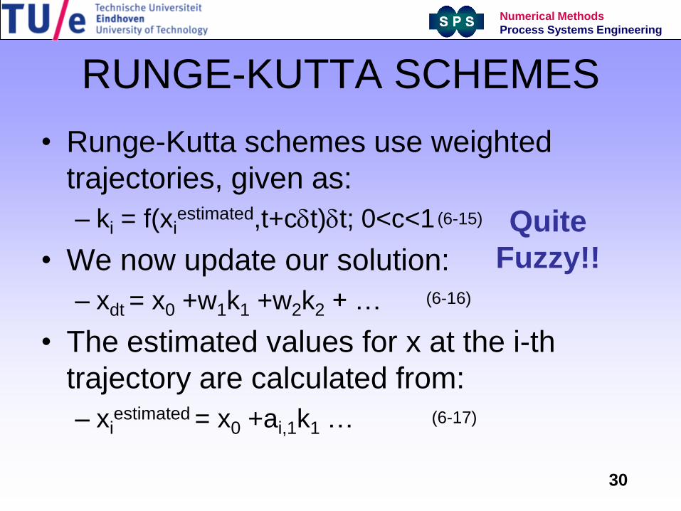
RUNGE-KUTTA SCHEMES
• Runge-Kutta schemes use weighted
trajectories, given as:
– ki = f(xiestimated,t+cdt)dt; 0<c<1
• We now update our solution:
– xdt = x0 +w1k1 +w2k2 + …
• The estimated values for x at the i-th
trajectory are calculated from:
– xiestimated = x0 +ai,1k1 …
Quite
Fuzzy!!
(6-15)
(6-16)
(6-17)

31
Numerical Methods
Process Systems Engineering
RK 2ND ORDER TIME STEPPING SCHEME
• For the 2nd order RK scheme we need to
evaluate 2 trajectories:
• xdt = x0 +w1k1 +w2k2
• Where k1 = f(x0,t)dt
• And k2 =f (x0 + a2,1k1,t+c2dt)dt
• We must choose the weights (w1,w2, a2,1)
and the position c2 such that we get an
error of O(dt3) over asingle time step!
(6-18)
(6-19)
(6-20)

32
Numerical Methods
Process Systems Engineering
RK 2ND ORDER TIME STEPPING SCHEME
• After expanding a function x into a Taylor
series we have to compare the following
outcomes:
)(!2
)()),((),(
)()(
32
000
32
22
2
1,2210
tOt
ftxffttxfxx
tOtfcwtffawwwfxx
ix
ix
w
dd
d
ddd
++++=
+++++=
21
22
21
1,22
21 1)(
=
=
=+
cw
aw
ww
Three eqn. With
4 unknowns
Set c2 =1 w1 = w2 = ½ a2,1 =1
Crank-Nicholson scheme
Set c2 = ½ w1 = 0 w2 = 1 a2,1 = ½
Euler mid point scheme
(6-21)
(6-22)
(6-23)

33
Numerical Methods
Process Systems Engineering
MATLAB CODE FOR 4TH
ORDER RKfunction [x,t] = RungeKutta_4(MyFunc,InitialValues,Start,Finish,Nsteps)
x(:,1) = InitialValues'
t(1) = Start;
dt = (Finish - Start)/Nsteps;
for i = 1:Nsteps
k1 = feval(MyFunc,x(:,i),t(i))*dt;
k2 = feval(MyFunc,x(:,i) + k1/2,t(i) + dt/2)*dt;
k3 = feval(MyFunc,x(:,i) + k2/2,t(i) + dt/2)*dt;
k4 = feval(MyFunc,x(:,i)+k3,t(i) + dt)*dt;
t(i+1) = dt + t(i);
x(:,i+1) = (k1+2*k2+2*k3+k4)/6 + x(:,i);
end
t = t';
x = x';
return
34
Numerical Methods
Process Systems Engineering
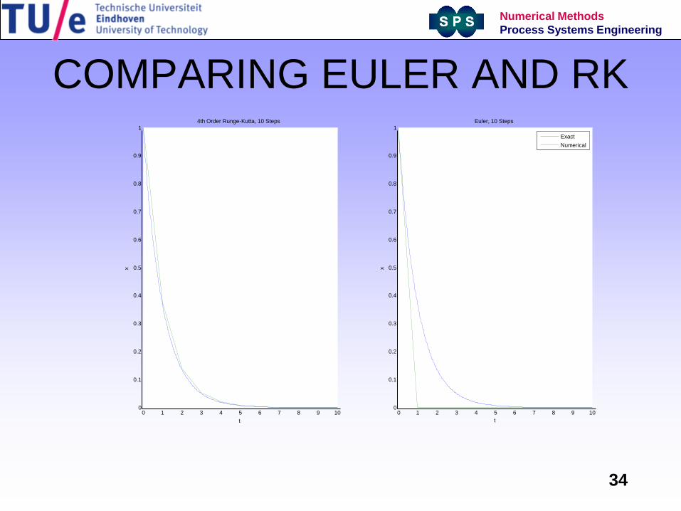
COMPARING EULER AND RK
0 1 2 3 4 5 6 7 8 9 100
0.1
0.2
0.3
0.4
0.5
0.6
0.7
0.8
0.9
1
t
x4th Order Runge-Kutta, 10 Steps
0 1 2 3 4 5 6 7 8 9 100
0.1
0.2
0.3
0.4
0.5
0.6
0.7
0.8
0.9
1
t
x
Euler, 10 Steps
Exact
Numerical
35
Numerical Methods
Process Systems Engineering
SUMMARY
• We looked at the Euler method, explicit and implicit
• We saw that an explicit method is conditionally stable
• We found that eigenvalues say something about stability
• Stiffness tells you if you can use an explicit or implicit
method (small or large time steps)
• Higher order methods provide large savings in
computational time.
• MATLAB has good solvers for ODE systems, e.g.
ODE15 and ODE45