Supplementary materials for this article are available at https:// doi.org/ 10.1007/ s13253-019-00377-z.

Understanding the Stochastic PartialDifferential Equation Approach to Smoothing

David L.Miller , Richard Glennie , and Andrew E. Seaton

Correlation and smoothness are terms used to describe a wide variety of randomquantities. In time, space, and many other domains, they both imply the same idea:quantities that occur closer together aremore similar than those further apart. Twopopularstatistical models that represent this idea are basis-penalty smoothers (Wood in Textsin statistical science, CRC Press, Boca Raton, 2017) and stochastic partial differentialequations (SPDEs) (Lindgren et al. in J R Stat Soc Series B (Stat Methodol) 73(4):423–498, 2011). In this paper, we discuss how the SPDE can be interpreted as a smoothingpenalty and can be fitted using the R package mgcv, allowing practitioners with existingknowledge of smoothing penalties to better understand the implementation and theorybehind the SPDE approach.

Supplementary materials accompanying this paper appear online.

Key Words: Smoothing; Stochastic partial differential equations; Generalized additivemodel; Spatial modelling; Basis-penalty smoothing.

1. INTRODUCTION

Data collected over space or time are often obtained with the desire to elicit an underlyingpattern. The stochastic partial differential equation (SPDE) approach introduced byLindgrenet al. (2011) and implemented in theR-INLA software package (Rue et al. 2009) is a flexible,efficient method to analyse such data. Despite this, wider application is inhibited by twoobstacles. First, the methods are presented using mathematical concepts and terms moreusually found in applied mathematics and physics, making it difficult for practitioners inother fields to understand and adapt these methods to their own needs. Second, availablesoftware implementations are difficult to customise without high-level technical knowledge,limiting application to only those models available in the software or specially requestedfrom software developers.

David L. Miller (B) and Richard Glennie and Andrew E. Seaton, Centre for Research into Ecological andEnvironmental Modelling and School of Mathematics and Statistics, University of St Andrews, St Andrews, Fife,Scotland, UK(E-mail: dave@ninepointeightone.net).

© 2019 The Author(s)Journal of Agricultural, Biological, and Environmental Statistics, Volume 25, Number 1, Pages 1–16https://doi.org/10.1007/s13253-019-00377-z

1

2 D. L. Miller et al.

Here, we aim to mitigate these two issues: we describe (i) how the SPDE model can beinterpreted as a basis-penalty smoother, a modelling framework more familiar to practition-ers who use smoothing techniques (Wood 2017), and (ii) how software to fit these smoothers(e.g. mgcv), regularly extended and customised for application, can be used to fit SPDEmodels or, to go further, used to incorporate SPDE methods into larger models.

In this paper, we consider the following situation. Let z(x) be a random variable observedat location x or time x , depending on the domain. A statistical model for z is constructed inthree components or terms: z(x) = η(x) + f (x) + ε(x). The first component, η(x), is thefixed effect, often a linear combination of observed covariates with unknown parameters.The third component, ε(x), represents the measurement error or unstructured error, oftenε(x) ∼ N (0, σ 2) for unknown parameter σ and every location x . The second component isa stochastic process, representing the structured dependence among observations: observa-tions made closer together in time or space are more likely to be similar than those furtherapart. A mathematically convenient and flexible model for this component is a Gaussianprocess (GP) with mean zero and covariance function c(xi , x j ) = Cov

{f (xi ), f (x j )

}. The

covariance function quantifies how related two values of f are at two locations. For fixedlocations {x1, . . . , xn}, the value of the GP at these locations, { f (x1), . . . , f (xn)}, is multi-variate Gaussian with mean zero and covariance matrix � with (i, j)th entry c(xi , x j ). Wecan extend this formulation to non-Gaussian responses by using a link function, g, so theresponse is then modelled with a specified distribution and a mean g−1(η(x) + f (x)).

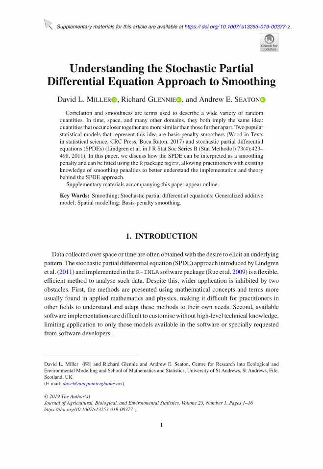
An example of this kind of data might be a time series of counts. The left panel ofFig. 1 shows human cases of campylobacteriosis (a common form of food poisoning, oftenoriginating in under-cooked poultry) in northern Québec, every 28 days from 1 January1990 to 31 October 2000. We may expect a given time period’s count to be similar toits neighbours (e.g. due to seasonal variation), so our aim is to build a model that cancapture this dependence. Using the above formulation, we model the counts as Poissonz(x) ∼ Po(exp( f (x))) where x represents time, z(x) is the number of cases at time x , f isa function of time representing the underlying process, and exp is the appropriate inverse

●

●

●

●

●

●

●

●

●

●

●

●

● ●

●

●

●

●

●

●

●

● ●

●

●

●

●

●

● ●

●

●

●

●

●

●

●

●

●

●

●

●

●

●

● ●

●

●

●

●

●

●

●

●

●

●

●

●

● ●

●

●

● ●

●

● ●

●

● ●

●

●

●

● ●

●

●

●

●

●

●

●

●

●

● ●

●

●

●

●

●

●

●

●

●

●

●

●

●

●

●

●

●

●

●

●

●

●

●

●

●

●

●

●

●

●

●

●

●

●

●

●

●

●

●

●

●

●

●

●

●

●

●

●

●

●

●

●

●

●

0

20

40

1990 1991 1992 1993 1994 1995 1996 1997 1998 1999 2000Time

Cam

pylo

bact

eros

is in

fect

ions

44.0

44.5

45.0

45.5

46.0

46.5

58 59 60Longitude

Latit

ude

5 10 15

logchlorophyll A

Figure 1. Examples of data with underlying dependence between observations. Left shows counts of campy-lobacterosis infections in northern Québec, summarised every 28 days from 1 January 1990 to 31 October 2000.Right shows the raw log chlorophyll A in the Aral sea from the SeaWIFS satellite. In both cases, we can build amodel that takes into account the structure in the data.

Understanding the Stochastic Partial Differential Equation Approach 3

link function. Dependence structures become more complex when we move to a spatialdomain. The right panel of Fig. 1 shows remotely sensed log chlorophyll A levels in theAral sea, derived from satellite data. In this case, we expect that pixels close to each otherhave similar chlorophyll A levels. We now have x representing a location in space, and thelog chlorophyll A level at that location; z(x) is modelled by z(x) = f (x)+ε(x), where nowf is a two-dimensional stochastic process and ε(x) ∼ N (0, σ 2). We revisit these examplesin Sect. 4.

Including f in the model raises two issues: how to specify the covariance function c and,once specified, how to fit the model. There are many possible solutions to these questions,including the SPDE and smoothing penalty approaches, and each uses different theoreticaland numerical approximations; however, there is a common element: for observation loca-tions {x1, . . . , xn}, each method aims to define the covariance between these locations, byconstructing an approximation to the precision matrix, defined as the inverse of the covari-ance matrix (Q = �−1). The precision matrix is a fundamental quantity required to fitthese models (Simpson et al. 2012). The size of� andQmakes the necessary computationsexpensive, in particular, if one of these matrices needs to be inverted so as to compute theother. It is in trying to avoid this computational burden that approximations are used.

TheSPDEapproach provides amethod to approximateQwithout the common substantialcomputational burden. The SPDE is an equation to be solved. Solutions to this equation arestochastic processes whose covariance structure is chosen to satisfy the relationship theSPDE specifies. The SPDE approach involves finding an SPDE whose solutions have thecovariance structure, and implied precision matrix, that is desired for f . Lindgren et al.(2011) show how to find an approximate solution to the SPDE by representing f as a sumof basis functions multiplied by coefficients; this provides a computationally efficient wayto compute Q: Lindgren et al. (2011) show that the coefficients of these basis functionsform a Gaussian Markov random field, for which methods for fast computation of precisionmatrices already exist (Rue and Held 2005). These computations make it possible to fitmodels quickly using integrated nested Laplace approximations (INLA; Rue et al. 2009).

Rue et al. (2017) is a comprehensive review of INLA that defines the class of latentGaussian models with additive linear predictors which INLA is designed to fit. They alsointroduce Gaussian Markov random fields and their properties that lead to efficient compu-tation, a key feature of the SPDE approach. Bakka et al. (2018) review the use of INLA forspatial modelling with a focus on the SPDE approach. They give an intuition for the methodby introducing the notion of a “discretised” differential operator and describing the finiteelement methods that are used to solve the SPDE (Brenner and Scott 2007; Bakka 2018).See also Krainski et al. (2019) for a collection of worked examples of modelling with SPDEsusing R-INLA, Wood (2019) for an approach to nested Laplace approximations withoutsparse Gaussian Markov random field structures, and Blangiardo and Cameletti (2015)for a comprehensive textbook on spatio-temporal modelling with R-INLA. We note thatthe R-INLA implementation of the SPDE approach has been applied in a wide variety ofdomains such as spatial epidemiology (Arab 2015), species distribution mapping (de Riveraet al. 2018), spatial point processes (Simpson et al. 2016; Yuan et al. 2017; Soriano-Redondoet al. 2019), and environmental science (Huang et al. 2017), to name just a few examples.

4 D. L. Miller et al.

Our presentation here differs from the above resources in that we explicitly draw links withanother well-known modelling framework.

The basis-penalty smoothing approach (Wood 2017) is similar to the SPDE approach:the function f is a sum of basis functions multiplied by coefficients. Rather than specify anSPDE and deduce a covariance structure between the coefficients, a smoothing penalty isused to induce correlation between the coefficients. This penalty measures how smooth f isin its domain; intuitively, if f changes more smoothly then values of f at nearby locationsare more correlated. Jointly optimising a measure of fit (sum of squares or log-likelihood)and smoothing penalty leads to an optimal curve, the smoothing spline (Wahba 1990). Thisis a well-established approach with several excellent introductory resources (Hastie andTibshirani 1990; Ramsay and Silverman 2005; Wood 2017) and has been applied in manyspatio-temporal modelling contexts (recent examples include Wood et al. (2017), Simpson(2018), Pedersen et al. (2019))

There is a direct correspondence between smoothing splines and stochastic processes(Kimeldorf and Wahba 1970): the smoothing spline is a minimum variance unbiased linearestimator of the posterior mean of the stochastic process. For a stochastic process witha given covariance function, there is a corresponding SPDE and smoothing penalty suchthat one can estimate the posterior mean of f using the SPDE approach or the basis-penalty approach: both methods estimate the same quantity with the only differences beingin numerical approximations and terminology. This means that the SPDE can be interpretedas a smoothing penalty and vice versa.

This equivalence has been confirmed by Fahrmeir and Lang (2001), Lindgren and Rue(2008), and Yue et al. (2014) who show how basis-penalty smoothers in a Bayesian frame-work can be interpreted within the SPDE paradigm. Simpson et al. (2012) remark thatthe SPDE formulation is useful because it provides those with a background in physics orapplied mathematics a way to understand and apply the model. In contrast, less emphasishas been placed on discussing this equivalence the other way around: SPDE methods canbe formulated as basis-penalty smoothers. The SPDE formulation can seem opaque andfundamentally different for those unfamiliar with the mathematical concepts used. For thisreason, showing the approach within the familiar smoothing framework demystifies theworkings of the model and allows researchers in other fields to understand, adapt, and usethe methods. We note that our approach is aligned with the general aim of emphasisinglinks between Gaussian processes and the reproducing kernel Hilbert spaces theory thatunderpins the basis-penalty smoothing approach (Kanagawa et al. 2018), although here wetake a more applied perspective.

Our aim in this paper is to show that the SPDE model as introduced by Lindgren et al.(2011) (usually fitted using R-INLA) can be described as a basis-penalty smoother and fit-ted using mgcv. To do this, we first describe the SPDEmethod for those unfamiliar with themathematical concepts used, highlighting the key steps in the method. Afterwards, we showthe equivalences and differences between the SPDEmethod and the analogous basis-penaltysmoother.

Understanding the Stochastic Partial Differential Equation Approach 5

2. THE SPDE APPROACH

2.1. WHAT IS AN SPDE?

A stochastic partial differential equation involves stochastic processes and differen-tial operators. Examples of differential operators (D) are the first derivative, the secondderivative, the gradient operator in two dimensions or the Laplacian in two dimensions.Combinations of these are also differential operators, e.g. D = d/dx + d2/dx2 such thatD f = d f/dx + d2 f/dx2 for a function f . Here, we consider only linear differential opera-tors, that is, D f is a linear combination of derivatives of f , of different orders. Differentialoperators of stochastic processes can be treated similarly to those applied to ordinary func-tions, there is one key difference that we will highlight below. Overall, an SPDE states thatthe differential of a function f is equal to some known stochastic process, most commonlythe white noise process, ε. The white noise process is completely uncorrelated, and ε(x) isa normal random variable with mean zero and finite variance for every x .

In general, the SPDE states that D f = ε for some differential operator D. A stochasticprocess, f , is called a solution to the SPDE if it satisfies this equation. Consider an example,let D be the first derivative of the function. The SPDE D f = ε, therefore, states that the firstderivative of f has mean zero and finite variance at every point; furthermore, it states thatthe value of the derivative at points x and y is uncorrelated for all x �= y. Approximately,this means that for a small δ and point x , f (x + δ) = f (x)+ ξ where ξ is a normal randomvariable. Consider if the SPDE has a parameter τ such that D f = ε/τ such that τ controlsthe variance in the white noise process. This means that changes in f are more variablewhen τ is reduced and less variable for higher τ . In other words, the parameters of theSPDE control the smoothness of f . It is important to note that here the term “smoothness”is not used in a mathematical way, meaning differentiability, nor in a strictly statistical way,referring to correlation range, but in a qualitative way—when we speak of differentiabilityor correlation we shall use those terms explicitly.

For a given D, the mathematical form of the solution to the SPDE D f = ε is known:f (x) = ∫

w(x − u)ε(u) du where w is a function you can derive given you know D.The function w is called Green’s function; in the appendix (Proposition 1), we show howthis function is derived from D. Intuitively, w acts as a weighting function such that thevalue of the stochastic process at x is a weighted sum over the white noise process; this iscalled a convolution. Suppose w were set to give infinite weight to distance 0, w(0) = ∞,and zero elsewhere, w(d) = 0 for d �= 0, then f (x) = ε(x): f is just the white noiseprocess, completely uncorrelated. Alternatively, if w gave equal weight to all distances, e.g.w(d) = 1 for all d, then f (x) would be constant, perfectly correlated. Between these twoextremes are weighting functions that reproduce correlations over different ranges. It canbe shown that the covariance function is given by c(x, y) = ∫

w(x − u)w(y − u) du, seeappendix (Proposition 2) for the derivation.

In summary, the solutions to the SPDE D f = ε have a covariance structure that is inducedby the choice of D. This means that one could describe a system using an SPDE and thendeduce the associated covariance function from it. The power of the SPDE approach isrealised by doing the opposite: find a D that induces the covariance function that you want.

6 D. L. Miller et al.

The power of finding the SPDE corresponding to a desired covariance function is that theprecision matrix can be efficiently computed using the SPDE.

2.2. SOLVING THE SPDE

The SPDE involves applying a differential operator D to a stochastic process, f , butthis cannot be done in the same way as when you apply D to a known function. This isbecause f is random and, in many cases, realisations of f will not be suitably differen-tiable. For example, the Brownian motion stochastic process has a derivative equal to thewhite noise process, but it is also known that simulated trajectories of Brownian motionare nowhere differentiable. D f = ε is a convenient shorthand way to think about theSPDE, but technically, the SPDE only has meaning when stated in an integral form. Thatis, D f = ε means that we require

∫D f (x)φ(x) dx = ∫

ε(x)φ(x) dx for every func-tion φ with compact support. The function φ is often called the test function. For brevity,let 〈 f, g〉 = ∫

f (x)g(x) dx and so the integral form is 〈D f, φ〉 = 〈ε, φ〉. The notation〈 f, g〉 is called the inner product of f, g; it has many nice mathematical properties, includ-ing being linear, that is 〈∑n

i=1 ai fi ,∑m

j=1 bi gi 〉 = ∑ni=1

∑mj=1 ai b j 〈 fi , g j 〉 for functions

f1, . . . , fn, g1, . . . , gm and constants a1, . . . , an, b1, . . . , bm .In the integral form, the equation makes sense because any stochastic process can be

integrated, but not every one can be differentiated. By requiring the equation to hold forevery φ, we require the left-hand stochastic process D f and the right-hand process ε tohave the same integral, no matter how we average over space. For example, if the stochasticprocesses were one-dimensional, we could split the real line into intervals [n, n + 1] andselect a function φn to be one on this interval and zero outside. Since the integral equationmust hold for all such functions, we therefore require D f to have the same average valueas ε on each and every interval.

Given an SPDE, Lindgren et al. (2011) show how to derive an approximate solution usingthe finite element method. The domain (e.g. time or space) is split into “elements”, e.g. agrid or a triangulation, often called a mesh. To each point j = 1, . . . , M on this mesh, abasis function ψ j is associated. The solution to the SPDE is then a weighted sum of thebasis functions and random variables β j : f (x) = ∑M

j=1 β jψ j (x).

The integral form of the SPDE then implies that for any function φ,∑M

j=1 β j 〈Dψ j , φ〉 =〈ε, φ〉. We cannot, however, check this equation for infinitely many test functions φ, soinstead we restrict to only testing with the functions that can be written in our chosenbasis. As D is a linear operator, this is equivalent to solving the system of equations∑M

j=1 β j 〈Dψ j , ψi 〉 = 〈ε, ψi 〉 for every i = 1, . . . , M . This system can be written as amatrix equation: Pβ = e where P has (i, j)th entry 〈Dψi , ψ j 〉 and e has j th entry 〈ε, ψ j 〉.

To summarise, the SPDE is written in an integral form, sometimes using inner products,since stochastic processes are well defined when integrated but not when differentiated.Given this, the solution is represented in a chosen basis. The integral form is then solved byconsidering only test functions within that basis. This leads to a matrix equation involvingthe coefficients β, the matrix P, and the random vector e. The random vector e has knowndistribution, because it depends only on the basis functions and thewhite noise process: e hasa multivariate Gaussian distribution with mean zero and a precision matrix Qe where Q−1

e

Understanding the Stochastic Partial Differential Equation Approach 7

has (i, j)th entry 〈ψi , ψ j 〉. It follows fromPβ = e that β ∼ N (0,Q−1)whereQ = PTQeP.The SPDE is therefore a way to specify a prior for β.

This provides an approximate solution to the SPDE. For example, given an SPDE, one canuse the finite element method to compute Q and therefore simulate β̃ from a multivariateGaussian distribution with precision Q. The function f̃ = ∑M

j=1 β̃ jψ j would then be arealisation from a stochastic process which is a solution to the SPDE, a stochastic processwith the covariance structure implied by D.

2.3. MATÉRN SPDE

The focus of Lindgren et al. (2011) and the covariance function most commonly used inthe R-INLA software is the Matérn covariance function. The Matérn covariance functionis considered a flexible model for the dependencies found in real-world observations: it hasthe form c(x, y) = 21−ν

(4π)d/2κ2τ 2�(ν)(κ‖x − y‖)ν Kν(κ‖x − y‖) where ν, κ, τ are parameters,

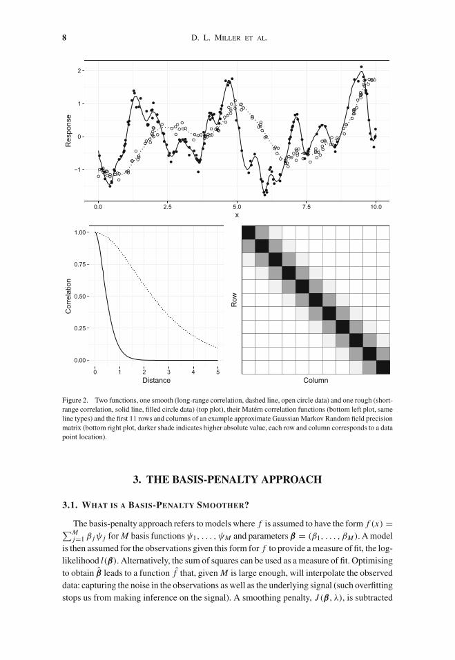
Kν is the modified Bessel function of the second kind, and d is the dimension of the domain.Figure 2 shows realisations from two stochastic processes withMatérn covariance functionsin one dimension, one with a longer correlation range than the other.

It is difficult to fit models with this covariance structure due to the computational issuesmentioned above. Lindgren et al. (2011) apply the finite element method to approximatestochastic processes with Matérn covariance (a comparison of the notation used in Sect. 2.2and that used in Lindgren et al. (2011) is given in the appendix, Sect. 5). To do this, theypresent the differential operator that corresponds to this covariance function: D = (κ2 −�)α/2τ where α = ν − d/2.

When α �= 2, this is called a fractional differential operator; for this paper, we consideronly the case when α = 2 and so D is again a linear differential operator. In practice, α ispoorly identified and difficult to estimate from data, so its value is often assumed to be fixed(Zhang 2004).

Lindgren et al. (2011) solve the SPDE κ2 f −� f = ε/τ using the finite element method.By deriving the weighting function and computing the covariance from this SPDE, Whittle(1954) shows that the solutions have Matérn covariance, as desired. In other words, theprecision matrix computed from the finite element method is an approximation to the pre-cision matrix one would obtain if you computed the variance–covariance matrix � withthe Matérn covariance function and then, at great computational cost, inverted this matrix.Figure 2 shows a subview of the approximate precision matrix: the matrix is mostly filledwith zeroes, with nonzero values occurring on three bands down the diagonal. This is anexample of a sparse matrix; computations with these matrices are efficient because manyof the computations ordinarily required can be omitted as it is known the matrix is mostlyzeroes.

To use the finite element method, one must chose a mesh, a grid, or triangulation, overthe domain and a basis to define on this mesh. The default choice in R-INLA is to use aregular grid in 1D (or a constrained Delaunay triangulation in 2D) to produce a mesh andthen define piecewise linear basis functions (specifically, linear B-spline basis functions) onthis mesh.

8 D. L. Miller et al.

●

●

●

●

●

●

●●

●

●

●

●

●

●

●

●

●

●

●

●

●

●●

●

●

●

●

●

●

●

●

●

●

●●

●

●

●

●

●

●

●

●

●

●

●

●

● ●

●

●

●

●

●

●

●

● ●

●

●

●

●

●

●

●

●

●

●

●

●

●

●

●

●

●

●

●

●

●

●

●

●

●

●

●

●

●

●

●

●●

●

●

●

●

●

●

●

●

●

●

●

●

●

●

● ●

●

●

●

●

●

●

●

●

●

●

●

●●

●

●

●

●

●

●

●

●

●

●

●

●

●

●

●

●

●

●

●

●

●

●

●

●

●

●

●

●

●

●

●

●

●

●

●

●

●

●●

●

●

●

●●

●

●

●

●

●

●

●

●

●

●

●

●●

●

●

●

●

●●

●

●

●

●

●

● ●

●

●

●

●

●

●

●

●

●

●

●

●

●

●

●

●

●

●●

●

●

●

●

●

●

●

●

●

●

●

●

●

●

●

●●

●●

●

●

●

●

●

●●

●

●

●

●

●

●

●

●

●

●

●

●

●

●

●●

●

●

●

●

●

●

●

●

●

●

●

● ●●

●

●

●

●

●

●

●

●

●●

●

●

●

●

●

● ●

●

●

●

●

●

●

●

●

●

●

●

●

●

●

●

●

●

●

−1

0

1

2

0.0 2.5 5.0 7.5 10.0x

Res

pons

e

0.00

0.25

0.50

0.75

1.00

0 1 2 3 4 5Distance

Cor

rela

tion

Column

Row

Figure 2. Two functions, one smooth (long-range correlation, dashed line, open circle data) and one rough (short-range correlation, solid line, filled circle data) (top plot), their Matérn correlation functions (bottom left plot, sameline types) and the first 11 rows and columns of an example approximate Gaussian Markov Random field precisionmatrix (bottom right plot, darker shade indicates higher absolute value, each row and column corresponds to a datapoint location).

3. THE BASIS-PENALTY APPROACH

3.1. WHAT IS A BASIS-PENALTY SMOOTHER?

The basis-penalty approach refers tomodels where f is assumed to have the form f (x) =∑Mj=1 β jψ j for M basis functionsψ1, . . . , ψM and parameters β = (β1, . . . , βM ). Amodel

is then assumed for the observations given this form for f to provide ameasure of fit, the log-likelihood l(β). Alternatively, the sum of squares can be used as a measure of fit. Optimisingto obtain β̂ leads to a function f̂ that, given M is large enough, will interpolate the observeddata: capturing the noise in the observations as well as the underlying signal (such overfittingstops us from making inference on the signal). A smoothing penalty, J (β, λ), is subtracted

Understanding the Stochastic Partial Differential Equation Approach 9

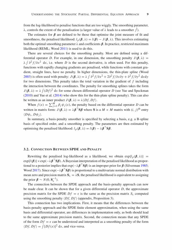
from the log-likelihood to penalise functions that are too wiggly. The smoothing parameter,λ, controls the extent of the penalisation (a larger value of λ leads to a smoother f̂ ).

The estimates for β are defined to be those that optimise the joint measure of fit andsmoothness, the penalised likelihood: l p(β, λ) = l(β) − J (β, λ). This involves estimatingboth the optimal smoothing parameter λ and coefficients β. In practice, restricted maximumlikelihood (REML; Wood 2011) is used to do this.

There are several choices for the smoothing penalty. Most are defined using a dif-ferential operator D. For example, in one dimension, the smoothing penalty J (β, λ) =λ

∫∂2 f/∂x2 dx , i.e. where D is the second derivative, is often used. For this penalty,

functions with rapidly changing gradients are penalised, while functions with constant gra-dient, straight lines, have no penalty. In higher dimensions, the thin-plate spline (Wood2003) is often used with penalty: J (β, λ) = λ

∫∂2 f/∂x2 + 2∂2 f/∂x∂y + ∂2 f/∂y2 dxdy

for two dimensions. This penalty takes the total variation in the gradient of f includingthe interaction between the coordinates. The penalty for smoothing splines takes the formJ (β, λ) = λ

∫(D f )2 dx for some chosen differential operator D (see Yue and Speckman

(2010) and Yue et al. (2014) who show this for the thin-plate spline penalty). This can alsobe written as an inner product J (β, λ) = λ〈D f, D f 〉.

When f (x) = ∑Mj=1 β jψ j (x), the penalty based on the differential operator D can be

written in matrix form: J (β, λ) = λβ�Sβ where S is a M × M matrix with (i, j)th entry〈Dψi , Dψ j 〉.

In summary, a basis-penalty smoother is specified by selecting a basis, e.g. a B-splinebasis of specified order, and a smoothing penalty. The parameters are then estimated byoptimising the penalised likelihood: l p(β, λ) = l(β) − λβ�Sβ.

3.2. CONNECTION BETWEEN SPDE AND PENALTY

Rewriting the penalised log-likelihood as a likelihood, we obtain exp{l p(β, λ)} =exp{l(β)}×exp(−λβ�Sβ). A Bayesian interpretation of the penalised likelihood as propor-tional to a posterior implies that exp(−λβ�Sβ) is an improper prior for β (Silverman 1985;Wood 2017). Since exp(−λβ�Sβ) is proportional to a multivariate normal distribution withmean zero and precision matrix Sλ = λS, the penalised likelihood is equivalent to assigningthe prior β ∼ N (0,S−1

λ ).The connection between the SPDE approach and the basis-penalty approach can now

be made clear. It can be shown that for a given differential operator D, the approximateprecision matrix for the SPDE D f = ε is the same as the precision matrix Sλ computedusing the smoothing penalty 〈D f, D f 〉 (appendix, Proposition 3).

This connection has two implications. First, it means that the differences between thebasis-penalty approach and the SPDE finite element approximation, when using the samebasis and differential operator, are differences in implementation only, as both should leadto the same approximate precision matrix. Second, the connection means that any SPDEof the form D f = ε can be understood and interpreted as a smoothing penalty of the form〈D f, D f 〉 = ∫ {D f (x)}2 dx , and vice-versa.

10 D. L. Miller et al.

3.3. MATÉRN PENALTY

TheSPDE specified inLindgren et al. (2011) has the differential operator D = τ(κ2−�).Given the connection described above, this can be interpreted as a smoothing penalty:τ

∫(κ2 f − � f )2 dx . This penalty is different from those considered above because it

contains two smoothing parameters: τ and κ . This offers it more flexibility. The penalty canstill, however, be interpreted as such: it is a trade-off between the value of the function f andthe second derivative � f in each direction. As κ is increased, the value of κ2 f increases,meaning that � f can be higher, the function be less smooth, while keeping the penalty thesame. Alternatively, κ can be described as the inverse correlation range: higher values of κ

lead to less smooth functions meaning values of the function become less correlated. Thesmoothing parameter τ controls the overall smoothness of f .

TheMatérn penalty can be written in matrix form as above, but for computational conve-nience, it is first broken into three parts: 〈D f, D f 〉 = τ(κ4〈 f, f 〉+2κ2〈 f,∇ f 〉+〈∇ f,∇ f 〉).Notice that it appears that the Laplacian � has been replaced with the gradient opera-tor ∇: this relationship holds here using Green’s first identity and the Neumann boundarycondition, see Bakka et al. (2018) for more detail. This leads to the smoothing matrixS = τ(κ4C + 2κ2G1 + G2) where C, G1, G2 are all M × M matrices with (i, j)th entries〈ψi , ψ j 〉, 〈ψi ,∇ψ j 〉, and 〈∇ψi ,∇ψ j 〉, respectively. All of these matrices are sparse, andso computation of the smoothing penalty, β�Sβ, is computationally efficient. The matrix Sis equal to the matrix Q = P�QeP computed using the finite element method (Appendix,Proposition 3).

3.4. FITTING THE MATÉRN SPDE IN mgcv

The mgcv R package allows the specification of new basis-penalty smoothers by writ-ing new “smooth.construct” functions which build an appropriate design matrix(containing evaluations of the basis functions), penalty matrices, and other optionalcomponents. Within this framework, we can fit the SPDE model in mgcv providinga smooth.construct.spde.smooth.spec constructor. R-INLA provides helperfunctions to construct the required design and penaltymatrices. Here,we sketch an algorithmfor setting-up SPDE models in mgcv.

Given we have a response {yi ; i = 1, . . . , n} and covariates in an n × nc matrix Xc, weconstruct our model as follows.

1. Create a mesh using INLA::inla.mesh.1d or INLA::inla.mesh.2d.

2. CalculateC,G1 andG2 using INLA::inla.mesh.fem (c1, g1 and g2, respec-tively).

3. We need to connect the basis representation of f to the observation locations. Atpresent, β contains the value of f at each mesh point, not at each observationlocation. A matrix multiplication is used to project the values at all mesh pointsto the observations locations; it is called the projection matrix A (found usingINLA::inla.spde.make.A). The full design matrix X is then given by com-bining the fixed effects design matrix Xc and the contribution for f , A.

Understanding the Stochastic Partial Differential Equation Approach 11

4. Having constructed the designmatrix and penaltymatrices, useREML tofind optimalκ , τ and β subject to the penalty matrix κ4C + 2κ2G1 + G2. (Parametrisation forthis model in mgcv is given in Supplementary Material Section 4.)

As REML is an empirical Bayes procedure, we expect point estimates for β̂ to coincidefor the procedure outlined above and R-INLA. A uniform prior is implied for the smoothingparameters (τ or κ); R-INLA allows for similar estimation by just using the modes of thehyperparameters κ and τ (the int.strategy="eb" option). Proper priors could be usedif step (4), above, was replaced by an MCMC scheme.

4. EXAMPLES

We now compare the SPDE and basis-penalty models applied to three example datasets.We fitted the SPDE Matérn model in both R-INLA and mgcv. Code for these examples isavailable as supplementary material.

4.1. CAMPYLOBACTEROSIS CASES IN QUÉBEC

Ferland et al. (2006) analyse a time series of (human) cases of campylobacterosis innorthern Québec, with observations every 28 days from 1 January 1990 to 31 October 2000(140 observations). We modelled the number of infections as a function of time, using aPoisson response and a log link function. The model is fitted using three approaches (i) aMatérn basis-penalty smoother with 50 degree 2 B-splines, fitted with mgcv; (i i) a MatérnSPDE for f with a finite element basis of 50 degree 2 B-splines and penalised complexitypriors (Simpson et al. 2017) on smoothing parameters, fitted with R-INLA; (i i i) a basis-penalty smoother with penalty equal to the integral of the squared second derivative, using50 degree 2 B-splines fitted using mgcv.

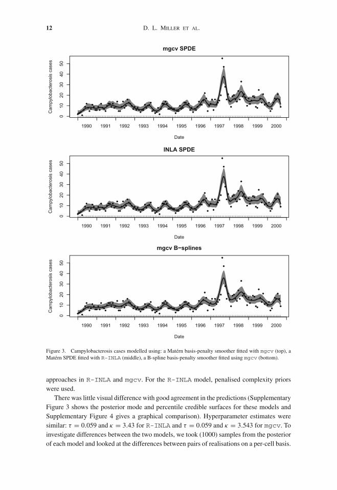
Fittedmodels are shown in Fig. 3. Results from the R-INLA and mgcv SPDE implemen-tations are very similar. This is supported by the similarity in the estimated hyperparameters(τ = 3.603 and κ = 0.429 for R-INLA, and τ = 3.252 and κ = 0.475 for mgcv). Thesquared second derivative penalty B-spline fit from mgcv is smoother than those from theSPDE-based methods.

4.2. ARAL SEA CHLOROPHYLL

Moving to a two-dimensional smoothing problem, we consider remotely sensed (log)chlorophyll from the Aral sea collected by the NASA SeaWifs satellite over a series of 8-day observation periods. The 496 observations used here are averages (from 1998 to 2002)of the 38th observation period. Data were taken from the gamair package (dataset aral)and consist of spatial coordinates and logarithm of chlorophyll concentration.

We built a mesh using fmesher::meshbuilder (Supplementary Figure 2) and gen-erated two-dimensional degree 1 B-splines. We consider the model yi = f (xi ) + ε forlocation xi with no fixed effects. We fitted the Matérn model using the SPDE and penalty

12 D. L. Miller et al.

mgcv SPDE

Date

Cam

pylo

bact

eros

is c

ases

1990 1991 1992 1993 1994 1995 1996 1997 1998 1999 2000

010

2030

4050

INLA SPDE

Date

Cam

pylo

bact

eros

is c

ases

1990 1991 1992 1993 1994 1995 1996 1997 1998 1999 2000

010

2030

4050

mgcv B−splines

Date

Cam

pylo

bact

eros

is c

ases

1990 1991 1992 1993 1994 1995 1996 1997 1998 1999 2000

010

2030

4050

Figure 3. Campylobacterosis cases modelled using: a Matérn basis-penalty smoother fitted with mgcv (top), aMatérn SPDE fitted with R-INLA (middle), a B-spline basis-penalty smoother fitted using mgcv (bottom).

approaches in R-INLA and mgcv. For the R-INLA model, penalised complexity priorswere used.

There was little visual difference with good agreement in the predictions (SupplementaryFigure 3 shows the posterior mode and percentile credible surfaces for these models andSupplementary Figure 4 gives a graphical comparison). Hyperparameter estimates weresimilar: τ = 0.059 and κ = 3.43 for R-INLA and τ = 0.059 and κ = 3.543 for mgcv. Toinvestigate differences between the two models, we took (1000) samples from the posteriorof each model and looked at the differences between pairs of realisations on a per-cell basis.

Understanding the Stochastic Partial Differential Equation Approach 13

44.0

44.5

45.0

45.5

46.0

46.5

58 59 60Longitude

Latit

ude

−0.15

−0.10

−0.05

0.00

0.05

Mean diff.

44.0

44.5

45.0

45.5

46.0

46.5

58 59 60Longitude

Latit

ude

0.6

0.8

1.0

1.2

1.4

SD of diff.

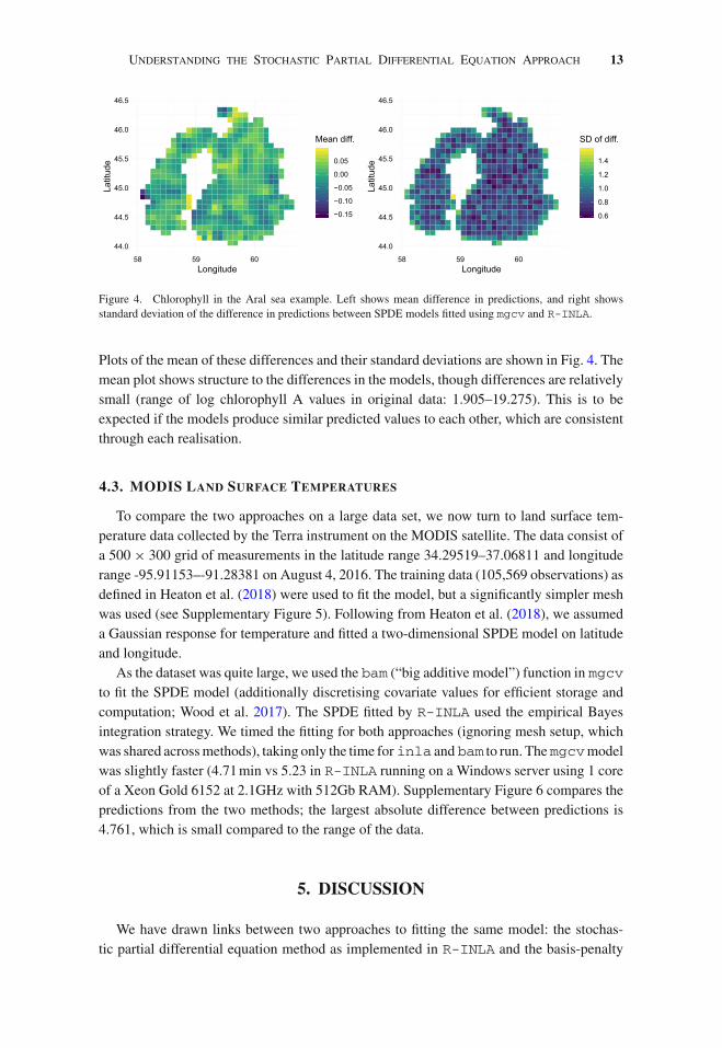
Figure 4. Chlorophyll in the Aral sea example. Left shows mean difference in predictions, and right showsstandard deviation of the difference in predictions between SPDE models fitted using mgcv and R-INLA.

Plots of the mean of these differences and their standard deviations are shown in Fig. 4. Themean plot shows structure to the differences in the models, though differences are relativelysmall (range of log chlorophyll A values in original data: 1.905–19.275). This is to beexpected if the models produce similar predicted values to each other, which are consistentthrough each realisation.

4.3. MODIS LAND SURFACE TEMPERATURES

To compare the two approaches on a large data set, we now turn to land surface tem-perature data collected by the Terra instrument on the MODIS satellite. The data consist ofa 500 × 300 grid of measurements in the latitude range 34.29519–37.06811 and longituderange -95.91153–-91.28381 on August 4, 2016. The training data (105,569 observations) asdefined in Heaton et al. (2018) were used to fit the model, but a significantly simpler meshwas used (see Supplementary Figure 5). Following from Heaton et al. (2018), we assumeda Gaussian response for temperature and fitted a two-dimensional SPDE model on latitudeand longitude.

As the dataset was quite large, we used the bam (“big additive model”) function in mgcvto fit the SPDE model (additionally discretising covariate values for efficient storage andcomputation; Wood et al. 2017). The SPDE fitted by R-INLA used the empirical Bayesintegration strategy. We timed the fitting for both approaches (ignoring mesh setup, whichwas shared acrossmethods), taking only the time for inla and bam to run. Themgcvmodelwas slightly faster (4.71min vs 5.23 in R-INLA running on a Windows server using 1 coreof a Xeon Gold 6152 at 2.1GHz with 512Gb RAM). Supplementary Figure 6 compares thepredictions from the two methods; the largest absolute difference between predictions is4.761, which is small compared to the range of the data.

5. DISCUSSION

We have drawn links between two approaches to fitting the same model: the stochas-tic partial differential equation method as implemented in R-INLA and the basis-penalty

14 D. L. Miller et al.

smoothing approach as fitted in mgcv. This paper aims tomake accessiblewhat is equivalentbetween the approaches, what is a matter of choice, and what is fundamentally different.Yue et al. (2014) show how splines can be specified using the SPDE approach, benefittingthose familiar with SPDEs. Here, we do the opposite for the benefit of those familiar withthe (penalised likelihood/empirical Bayes) GAM framework. Supplementary Figure 1 is aflow diagram showing the parallels between the smoothness and correlation approaches wehave discussed.

Similarities betweenmany smoothing techniques can be drawn. Smoothing splines, krig-ing, Gaussian Markov random fields, and SPDEs approximate similar models, but theirexplanations make it difficult for practitioners to appreciate their commonalities and deter-mine precisely what is a necessary and what is a coincidental association. Taking the pre-cision matrix as the common currency between these methods, a modelling frameworkemerges:

1. Choose a covariancemodel: explicitly, as in kriging, through the smoothness penaltyas with smoothing splines, or with an SPDE;

2. Approximate the precision matrix Q: reduce dimension (fixed rank kriging, thin-plate splines) or induce sparsity in Q ( B-splines, SPDE);

3. Draw approximate inference using a software implementation: e.g. with mgcv,MCMC (e.g. Stan (Carpenter et al. 2017); JAGS, (Plummer 2017)), R-INLA (Rueet al. 2009), lme4 (Bates et al. 2015) or TMB (Kristensen et al. 2016).

This paper is an example of comparing two methods according to this framework. Doingso for other smoothing methods will allow alternative modelling approaches to be comparedon the grounds of genuine differences: in the covariance function, in the approximation forQ, in the estimation procedure, or, simply, in the software implementation.

ACKNOWLEDGEMENTS

The authors wish to thank the editor and two anonymous reviewers for their constructive comments on the firstsubmission of the manuscript. They also thank Finn Lindgren for extremely helpful input and SimonWood for thesuggestion of the smoothing parameter parameterisation. The authors also thank Steve Buckland, David Borchers,and Joe Watson for their comments on the manuscript. DLM was funded by OPNAV N45 and the SURTASS LFASettlement Agreement, being managed by the US Navy’s Living Marine Resources Program under Contract No.N39430-17-C-1982.

Open Access This article is distributed under the terms of the Creative Commons Attribution 4.0 InternationalLicense (http://creativecommons.org/licenses/by/4.0/), which permits unrestricted use, distribution, and reproduc-tion in any medium, provided you give appropriate credit to the original author(s) and the source, provide a link tothe Creative Commons license, and indicate if changes were made.

[Received June 2019. Accepted September 2019. Published Online September 2019.]

Understanding the Stochastic Partial Differential Equation Approach 15

REFERENCES

Arab, A. (2015). Spatial and spatio-temporal models for modeling epidemiological data with excess zeros. Inter-

national Journal of Environmental Research and Public Health 12(9), 10536–10548.

Bakka, H. (2018). How to solve the stochastic partial differential equation that gives a Matérn random field usingthe finite element method. arXiv preprint arXiv:1803.03765.

Bakka, H., H. Rue, G.-A. Fuglstad, A. Riebler, D. Bolin, J. Illian, E. Krainski, D. Simpson, and F. Lindgren (2018).Spatialmodelingwith r-inla:A review.Wiley Interdisciplinary Reviews: Computational Statistics 10(6), e1443.

Bates, D., M.Mächler, B. Bolker, and S.Walker (2015). Fitting Linear Mixed-Effects Models Using lme4. Journal

of Statistical Software 67(1).

Blangiardo, M. and M. Cameletti (2015). Spatial and Spatio-temporal Bayesian Models with R-INLA. Wiley,Chichester, UK.

Brenner, S. and R. Scott (2007). The mathematical theory of finite element methods, Volume 15. Springer, NewYork, NY, USA.

Carpenter, B., A. Gelman, M. Hoffman, D. Lee, B. Goodrich, M. Betancourt, M. Brubaker, J. Guo, P. Li, andA. Riddell (2017). Stan: A Probabilistic Programming Language. Journal of Statistical Software 76(1), 1–32.

de Rivera, O. R., M. Blangiardo, A. López-Quílez, and I. Martín-Sanz (2018). Species distribution modellingthrough Bayesian hierarchical approach. Theoretical Ecology, 1–11.

Fahrmeir, L. and S. Lang (2001). Bayesian inference for generalized additive mixed models based on Markovrandom field priors. Journal of the Royal Statistical Society: Series C (Applied Statistics) 50(2), 201–220.

Ferland, R., A. Latour, and D. Oraichi (2006, November). Integer-Valued GARCH Process. Journal of Time Series

Analysis 27(6), 923–942.

Hastie, T. and R. Tibshirani (1990). Generalized Additive Models. Number 43 in Monographs on Statistics andApplied Probability. Chapman and Hall, London, UK.

Heaton, M. J., A. Datta, A. O. Finley, R. Furrer, J. Guinness, R. Guhaniyogi, F. Gerber, R. B. Gramacy, D. Ham-merling, M. Katzfuss, F. Lindgren, D. W. Nychka, F. Sun, and A. Zammit-Mangion (2018, December). A casestudy competition among methods for analyzing large spatial data. Journal of Agricultural, Biological and

Environmental Statistics.

Huang, J., B. P. Malone, B. Minasny, A. B. McBratney, and J. Triantafilis (2017). Evaluating a Bayesian modellingapproach (INLA-SPDE) for environmental mapping. Science of the Total Environment 609, 621–632.

Kanagawa, M., P. Hennig, D. Sejdinovic, and B. K. Sriperumbudur (2018, July). Gaussian Processes and KernelMethods: A Review on Connections and Equivalences. arXiv preprint arXiv:1807.02582.

Kimeldorf, G. S. and G. Wahba (1970). A correspondence between Bayesian estimation on stochastic processesand smoothing by splines. The Annals of Mathematical Statistics 41(2), 495–502.

Krainski, E., V. Gómez-Rubio, H. Bakka, A. Lenzi, D. Castro-Camilo, D. Simpson, F. Lindgren, and H. Rue(2019). Advanced Spatial Modeling with Stochastic Partial Differential Equations Using R and INLA. CRCPress, Boca Raton, FL, USA.

Kristensen, K., A. Nielsen, C. W. Berg, H. Skaug, and B. M. Bell (2016). TMB: Automatic differentiation andLaplace approximation. Journal of Statistical Software 70(5), 1–21.

Lindgren, F. and H. Rue (2008). On the second-order random walk model for irregular locations. Scandinavian

journal of statistics 35(4), 691–700.

Lindgren, F., H. Rue, and J. Lindström (2011). An explicit link between Gaussian fields and Gaussian Markovrandom fields: the stochastic partial differential equation approach. Journal of the Royal Statistical Society:

Series B (Statistical Methodology) 73(4), 423–498.

Pedersen, E. J., D. L. Miller, G. L. Simpson, and N. Ross (2019). Hierarchical generalized additive models inecology: an introduction with mgcv. PeerJ 7, e6876.

Plummer, M. (2017). JAGS Version 4.3.0 user manual.

Ramsay, J. and B. W. Silverman (2005). Functional Data Analysis (2 ed.). Springer Series in Statistics. New York:Springer-Verlag.

16 D. L. Miller et al.

Rue, H. and L. Held (2005). Gaussian Markov Random Fields: Theory and Applications, Volume 104 of Mono-graphs on Statistics and Applied Probability. Chapman & Hall, London, UK.

Rue, H., S. Martino, and N. Chopin (2009). Approximate Bayesian inference for latent Gaussian models byusing integrated nested Laplace approximations. Journal of the Royal Statistical Society: Series B (Statistical

Methodology) 71(2), 319–392.

Rue, H., A. Riebler, S. H. Sørbye, J. B. Illian, D. P. Simpson, and F. K. Lindgren (2017). Bayesian computing withinla: A review. Annual Review of Statistics and Its Application 4(1), 395–421.

Silverman, B.W. (1985). Some aspects of the spline smoothing approach to non-parametric regression curve fitting.Journal of the Royal Statistical Society. Series B (Methodological) 47(1), 1–52.

Simpson, D., J. B. Illian, F. Lindgren, S. H. Sørbye, and H. Rue (2016). Going off grid: computationally efficientinference for log-Gaussian Cox processes. Biometrika 103(1), 49–70.

Simpson, D., F. Lindgren, and H. Rue (2012). In order to make spatial statistics computationally feasible, we needto forget about the covariance function. Environmetrics 23(1), 65–74.

Simpson, D., H. Rue, A. Riebler, T. G. Martins, and S. H. Sørbye (2017). Penalising model component complexity:a principled, practical approach to constructing priors. Statistical Science 32(1), 1–28.

Simpson, G. L. (2018). Modelling Palaeoecological Time Series Using Generalised Additive Models. Frontiers in

Ecology and Evolution 6.

Soriano-Redondo, A., C. M. Jones-Todd, S. Bearhop, G. M. Hilton, L. Lock, A. Stanbury, S. C. Votier, andJ. B. Illian (2019). Understanding species distribution in dynamic populations: a new approach using spatio-temporal point process models. Ecography 42(6), 1092–1102.

Wahba, G. (1990). Spline models for observational data. SIAM, Philadelphia, PA, USA.

Whittle, P. (1954). On stationary processes in the plane. Biometrika 41(3-4), 434–449.

Wood, S. N. (2003). Thin plate regression splines. Journal of the Royal Statistical Society: Series B (StatisticalMethodology) 65(1), 95–114.

Wood, S. N. (2011). Fast stable restricted maximum likelihood andmarginal likelihood estimation of semiparamet-ric generalized linearmodels. Journal of the Royal Statistical Society: Series B (Statistical Methodology) 73(1),3–36.

Wood, S. N. (2017). Generalized Additive Models. An Introduction with R (2nd ed.). Texts in Statistical Science.CRC Press, Boca Raton, FL, USA.

Wood, S. N. (2019). Simplified integrated nested Laplace approximation. Biometrika.

Wood, S. N., Z. Li, G. Shaddick, andN. H. Augustin (2017, July). GeneralizedAdditiveModels for Gigadata:Mod-eling the U.K. Black Smoke Network Daily Data. Journal of the American Statistical Association 112(519),1199–1210.

Yuan, Y., F. E. Bachl, F. Lindgren, D. L. Borchers, J. B. Illian, S. T. Buckland, H. Rue, T. Gerrodette, et al. (2017).Point process models for spatio-temporal distance sampling data from a large-scale survey of blue whales.The Annals of Applied Statistics 11(4), 2270–2297.

Yue, Y. and P. L. Speckman (2010). Nonstationary spatial Gaussian Markov random fields. Journal of Computa-

tional and Graphical Statistics 19(1), 96–116.

Yue, Y. R., D. Simpson, F. Lindgren, and H. Rue (2014). Bayesian adaptive smoothing splines using stochasticdifferential equations. Bayesian Analysis 9(2), 397–424.

Zhang, H. (2004). Inconsistent estimation and asymptotically equal interpolations in model-based geostatistics.Journal of the American Statistical Association 99(465), 250–261.

Publisher’s Note Springer Nature remains neutral with regard to jurisdictional claims in publishedmaps and institutional affiliations.