Embed Size (px)
Citation preview

Analytical and numerical methods for pricingfinancial derivatives
Daniel Sevcovic
Comenius University, Bratislava
Conducted seminars: Beata Stehlıkova
Lectures at Masaryk University, 2011
Lectures by D. Sevcovic, Comenius University, Bratislava, Slovak republicAnalytical and numerical methods for pricing financial derivatives

Outline
1 Financial derivatives as tool for protecting volatile underlyingassets
2 Stochastic differential calculus, Ito’s lemma, Ito’s integral3 Pricing European type of options - Black–Scholes model4 Explicit and implicit schemes for pricing European type of
options5 Sensitivity analysis – dependence of the option price on
parameters6 Path dependent exotic options – Asian and barrier options7 Pricing American type options – free boundary problems and
numerical methods8 Nonlinear extensions of the Black-Scholes theory and
numerical approximation9 Modeling of stochastic interest rates and interest rate
derivatives10 Appendix: Fokker–Planck equation and multidimensional Ito’s
lemmaLectures by D. Sevcovic, Comenius University, Bratislava, Slovak republicAnalytical and numerical methods for pricing financial derivatives

The content of these lectures is based on the textbooks:
1 D. Sevcovic, B. Stehlıkova, K. Mikula:Analytical and numerical methods for pricing financial
derivatives.
Nova Science Publishers, Inc., Hauppauge, 2011. ISBN: 978-1-61728-780-0
2 D. Sevcovic, B. Stehlıkova, K. Mikula:Analyticke a numericke metody ocenovania financnych
derivatov,Nakladatelstvo STU, Bratislava 2009, ISBN 978-80-227-3014-3
3 P. Wilmott, J. Dewynne, J., S.D. Howison:Option Pricing: Mathematical Models and Computation,UK: Oxford Financial Press, 1995.
4 Hull, J. C.:Options, Futures and Other Derivative Securities.Prentice Hall, 1989.
The lecture slides are available for download fromwww.iam.fmph.uniba.sk/institute/sevcovic/derivaty
Lectures by D. Sevcovic, Comenius University, Bratislava, Slovak republicAnalytical and numerical methods for pricing financial derivatives

Black–Scholes model for pricing financial derivatives
Lecture 1
Stochastic character of assets (stocks, indices)
Financial derivatives as tool for protecting volatile portfolios
Examples of market data for Call and Put options
Lectures by D. Sevcovic, Comenius University, Bratislava, Slovak republicAnalytical and numerical methods for pricing financial derivatives
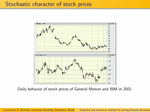
Stochastic character of stock prices
Daily behavior of stock prices of General Motors and IBM in 2001.
Lectures by D. Sevcovic, Comenius University, Bratislava, Slovak republicAnalytical and numerical methods for pricing financial derivatives

Stochastic character of stock prices
Daily behavior of stock prices of Microsoft and IBM in 2007 – 2008.
Volume of transactions is displayed in the bottom.
Lectures by D. Sevcovic, Comenius University, Bratislava, Slovak republicAnalytical and numerical methods for pricing financial derivatives

Stochastic character of indices
Daily behavior of Dow–Jones index
Precrisis period in the year 2000
Precrisis period 2007–2008.
Lectures by D. Sevcovic, Comenius University, Bratislava, Slovak republicAnalytical and numerical methods for pricing financial derivatives

Financial derivatives as a tool for protecting volatileportfolios
Forwardis an agreement between a writer (issuer) and a holderrepresenting the right and at the same time obligation topurchase assets at the specified time of maturity of a forwardat predetermined price E
Pricing forwards is relatively simple as soon as we know theforward interest rate r measuring the rate of the decrease of thevalue of money
Vf = E exp(−rT )
where E is the contracted expiration value of a forward at theexpiration time T . Here Vf denotes the present value of a forwardat the time when contract is signed
Lectures by D. Sevcovic, Comenius University, Bratislava, Slovak republicAnalytical and numerical methods for pricing financial derivatives

Financial derivatives as a tool for protecting volatileportfolios
Option (Call option)is an agreement between a writer (issuer) and a holderrepresenting the right BUT NOT the obligation to purchaseassets at the prescribed exercise price E at the specified timeof maturity T in the future
Pricing options is more involved as their price depends on:
Vc = function of E ,T , r , ..., ???
where E is the contracted expiration value of an options at theexpiration time T , Vc is the present value of a Call option at thetime when the contract is signed.
Lectures by D. Sevcovic, Comenius University, Bratislava, Slovak republicAnalytical and numerical methods for pricing financial derivatives

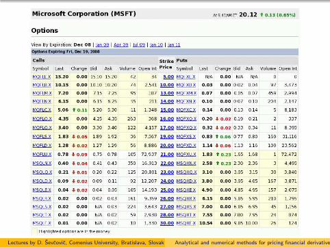
Call optionsSymbol Last Change Bid Ask Volume Open Int Strike Price
MQFLE.X 15.20 0.00 15.10 15.20 42 34 5.00MQFLB.X 10.15 0.00 10.10 10.20 74 2541 10.00MQFLM.X 7.20 0.00 7.15 7.25 95 187 13.00MQFLN.X 6.15 0.00 6.15 6.25 55 211 14.00MQFLC.X 5.06 0.11 5.20 5.30 11 1348 15.00MQFLO.X 4.35 0.00 4.25 4.35 263 368 16.00MQFLQ.X 3.40 0.00 3.30 3.40 122 4157 17.00MQFLS.X 1.83 0.05 1.89 1.92 36 7567 19.00MQFLU.X 1.28 0.02 1.27 1.29 56 8886 20.00MQFLU.X 0.78 0.09 0.75 0.78 105 72937 21.00MSQLN.X 0.40 0.04 0.41 0.43 350 16913 22.00MSQLQ.X 0.21 0.01 0.20 0.22 125 20801 23.00MSQLD.X 0.09 0.02 0.09 0.11 92 12207 24.00MSQLE.X 0.04 0.02 0.04 0.05 165 14193 25.00MSQLR.X 0.02 0.00 0.02 0.03 161 9359 26.00MSQLS.X 0.02 0.00 N/A 0.03 224 3643 27.00MSQLT.X 0.02 0.00 N/A 0.02 59 2938 28.00MSQLF.X 0.01 0.00 N/A 0.02 10 1330 30.00
Prices of Call options with different exercise (strike) prices E forMicrosoft stocks from 26. 11. 2008. with expiration 8.12.2008.The spot price S = 20.12The Call option price VC ≈ 1.28 > S − E = 20.12− 20 = 0.12
Lectures by D. Sevcovic, Comenius University, Bratislava, Slovak republicAnalytical and numerical methods for pricing financial derivatives
Lectures by D. Sevcovic, Comenius University, Bratislava, Slovak republicAnalytical and numerical methods for pricing financial derivatives

Intraday behavior (Feb. 7, 2011) of MSFT (Microsoft Inc.) stock.Source: Chicago Board Options Exchange: www.cboe.com
Lectures by D. Sevcovic, Comenius University, Bratislava, Slovak republicAnalytical and numerical methods for pricing financial derivatives

Call and Put option prices from Feb. 7, 2011, on MSFT (Microsoft Inc.)
stock with expiration July 2011 for various exercise (strike) prices E .Lectures by D. Sevcovic, Comenius University, Bratislava, Slovak republicAnalytical and numerical methods for pricing financial derivatives

Stochastic character of options
0 50 100 150 200 250 300 350
83
83.2
83.4
83.6
83.8
84
84.2
0 50 100 150 200 250 300 35013.5
13.75
14
14.25
14.5
14.75
15
15.25
0 50 100 150 200 250 300 35013.8
14
14.2
14.4
14.6
14.8
15
Figure: Top: Stock prices of IBM from 22. 5. 2002. Bottom: Bid andAsk prices of Call option for IBM stocks (left) and their arithmeticaverage value (right).
Lectures by D. Sevcovic, Comenius University, Bratislava, Slovak republicAnalytical and numerical methods for pricing financial derivatives

Financial derivatives as a tool for protecting volatileportfolios
A natural question arises:Although the time evolution of the asset price St as well as itsderivative (option) Vt is stochastic (volatile, unpredictable)CAN WE FIND A FUNCTIONAL DEPENDENCE
Vt = V (St , t)
relating the actual stock price St at time t and the price of itsderivative (like e.g. a Call option) Vt?
Lectures by D. Sevcovic, Comenius University, Bratislava, Slovak republicAnalytical and numerical methods for pricing financial derivatives

Financial derivatives as a tool for protecting volatileportfolios
This was a long standing problem in financial mathematicsuntil 1972. The answer is YES due to the pioneering work ofM.Scholes, F.Black and R.Merton.
M. Scholes and R. Merton were awarded the Price of theSwedish Bank for Economy in the memory of A. Nobel in1997 (Nobel price for Economy).
Lectures by D. Sevcovic, Comenius University, Bratislava, Slovak republicAnalytical and numerical methods for pricing financial derivatives

Financial derivatives as a tool for protecting volatileportfolios
The Black–Scholes formula
V = V (S , t;T ,E , r , σ)
where S = St is the spot (actual) price of an underlying asset,V = Vt is a the spot price of the option (Call or put) at time0 ≤ t ≤ T . Here T is the time of maturity, E is the exerciseprice, r > 0 is the interest rate of a secure bond, σ > 0 is thevolatility of underlying stochastic process of the asset price St .
Lectures by D. Sevcovic, Comenius University, Bratislava, Slovak republicAnalytical and numerical methods for pricing financial derivatives

Black–Scholes model for pricing financial derivatives
Lecture 2
Stochastic differential calculus
Wiener process, Brownian and geometric Brownian motion
Ito’s lemma, Ito’s integral
Lectures by D. Sevcovic, Comenius University, Bratislava, Slovak republicAnalytical and numerical methods for pricing financial derivatives

Stochastic differential calculus, Ito’s lemma
Stochastic process is a t - parametric system of randomvariables X (t), t ∈ I, where I is an interval or a discrete setof indices
Stochastic process X (t), t ∈ I is a Markov process with theproperty: given a value X (s), the subsequent values X (t) for
t > s may depend on X (s) but not on preceding values X (u)for u < s. More precisely,
If t ≥ s, then for conditional probabilities we have:
P(X (t) < x |X (s)) = P(X (t) < x |X (s),X (u))
for any u ≤ s.
Lectures by D. Sevcovic, Comenius University, Bratislava, Slovak republicAnalytical and numerical methods for pricing financial derivatives

Stochastic differential calculus, Ito’s lemma
a stochastic process X (t), t ≥ 0 is called the Brownianmotion if
i) all increments X (t +∆)− X (t) are normally distributed withthe mean value µ∆ and dispersion (or variance) σ2∆,
ii) for any division of times t0 = 0 < t1 < t2 < t3 < ... < tn theincrements X (t1)− X (t0),X (t2)− X (t1), ...,X (tn)− X (tn−1)are independent random variables
iii) X (0) = 0 and sample pathes are continuous almost surely
Brownian motion W (t), t ≥ 0 with the mean µ = 0 anddispersion σ2 = 1 is called Wiener process
Figure: Norbert Wiener (1884-1964) and Robert Brown (1773-1858).
Lectures by D. Sevcovic, Comenius University, Bratislava, Slovak republicAnalytical and numerical methods for pricing financial derivatives

Stochastic differential calculus, Ito’s lemma
Additive (or semigroup) property of the Brownian motion(BM) X (t), t ≥ 0 – Mean value
let 0 = t0 < t1 < ... < tn = t be any division of the interval [0, t].Then
X (t)− X (0) =n∑
i=1
X (ti)− X (ti−1).
Therefore the mean value E and variance Var of the left and righthand side have to be equal. By definition of the BM we have
E(X (t)− X (0)) = µ(t − 0) = µt .
On the other side we have (due to the linearity of the mean valueoperator):E(∑n
i=1 X (ti )− X (ti−1))
=∑n
i=1 E(X (ti )− X (ti−1)) =∑n
i=1 µ(ti − ti−1) = µt
In order to verify the equality we had to require thatincrements X (ti )− X (ti−1) have the mean valueE(X (ti)− X (ti−1)) = µ(ti − ti−1)
Lectures by D. Sevcovic, Comenius University, Bratislava, Slovak republicAnalytical and numerical methods for pricing financial derivatives

Stochastic differential calculus, Ito’s lemma
Additive (or semigroup) property of the Brownian motionX (t), t ≥ 0 – Variance
For dispersions of the random variables X (t)− X (0) and∑n
i=1(X (ti )− X (ti−1)) we have, by definition,
Var(X (t)− X (0)) = σ2(t − 0) = σ2t .
ReCall that for two random independent variables A,B it holds:Var(A + B) = Var(A) + Var(B). Hence, assuming independenceof increments X (ti)− X (ti−1) for different i = 1, 2, ..., n we have
Var(∑n
i=1 X (ti )− X (ti−1))
=∑n
i=1 Var(X (ti )− X (ti−1)) =∑n
i=1 σ2(ti − ti−1) = σ2t .
In order to verify the equality we had to require thatincrements X (ti )− X (ti−1) have the dispersion (variance)V (X (ti)− X (ti−1)) = σ2(ti − ti−1)
Lectures by D. Sevcovic, Comenius University, Bratislava, Slovak republicAnalytical and numerical methods for pricing financial derivatives

Stochastic differential calculus, Ito’s lemma
In summary:
The Brownian motion X (t), t ≥ 0 has the followingstochastic distribution:
X (t) ∼ N(µt, σ2t)
where N(mean, variance) stands for a normal random variablewith given mean and variance
The Wiener process W (t), t ≥ 0 (here µ = 0, σ2 = 1) hasthe following stochastic distribution:
W (t) ∼ N(0, t).
Moreover, dW (t) := W (t + dt)−W (t) ∼ N(0, dt), i.e.
dW (t) := W (t + dt)−W (t) = Φ√dt
where Φ ∼ N(0, 1).
Lectures by D. Sevcovic, Comenius University, Bratislava, Slovak republicAnalytical and numerical methods for pricing financial derivatives

Stochastic differential calculus, Ito’s lemma
0.2 0.4 0.6 0.8 1t
-2
-1
0
1
2
wHtL
0.2 0.4 0.6 0.8 1t
-2
-1
0
1
2
wHtL
Figure: Two randomly generated samples of a Wiener process.
0.2 0.4 0.6 0.8 1t
-2
-1
0
1
2
wHtL
Figure: Five random realizations of a Wiener process.
Lectures by D. Sevcovic, Comenius University, Bratislava, Slovak republicAnalytical and numerical methods for pricing financial derivatives

Stochastic differential calculus, Ito’s lemma
Since W (t) ∼ N(0, t) we have Var(W (t)) = t.
0 0.2 0.4 0.6 0.8 1t
0
0.2
0.4
0.6
0.8
1
VarHwHtLL
Figure: Time dependence of the variance Var(W (t)) for 1000 randomrealizations of a Wiener process W (t), t ≥ 0.
Lectures by D. Sevcovic, Comenius University, Bratislava, Slovak republicAnalytical and numerical methods for pricing financial derivatives

Stochastic differential calculus, Ito’s lemma
Relation between Brownian and Wiener process:
For a Brownian motion X (t), t ≥ 0 with parameters µ andσ we have, by definition,dX (t) = X (t + dt)− X (t) ∼ N(µdt, σ2dt) Therefore, if weconstruct the process
W (t) =X (t)− µt
σ
we have
dW (t) = W (t + dt)−W (t) =dX (t)− µdt
σ∼ N(0, dt),
i.e. W (t), t ≥ 0 is a Wiener process
Since X (t) = µt + σW (t) we may therefore write aStochastic differential equation
dX (t) = µdt + σdW (t) ,
Lectures by D. Sevcovic, Comenius University, Bratislava, Slovak republicAnalytical and numerical methods for pricing financial derivatives

Stochastic differential calculus, Ito’s lemma
Geometric Brownian motion
If X (t), t ≥ 0 is a Brownian motion with parameters µ and σ wedefine a new stochastic process Y (t), t ≥ 0 by taking
Y (t) = y0 exp(X (t))
where y0 is a given constant. The process Y (t), t ≥ 0 is calledthe Geometric Brownian motion.
Statistical properties of the Geometric Brownian motion
For simplicity, let us take y0 = 1. Then
W (t) =lnY (t)− µt
σ
is a Wiener process with W (t) ∼ N(0, t), i.e. we know itsdistribution function.
Lectures by D. Sevcovic, Comenius University, Bratislava, Slovak republicAnalytical and numerical methods for pricing financial derivatives
Stochastic differential calculus, Ito’s lemma
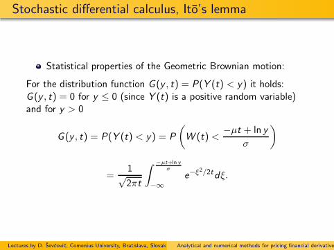
Statistical properties of the Geometric Brownian motion:
For the distribution function G (y , t) = P(Y (t) < y) it holds:G (y , t) = 0 for y ≤ 0 (since Y (t) is a positive random variable)and for y > 0
G (y , t) = P(Y (t) < y) = P
(
W (t) <−µt + ln y
σ
)
=1√2πt
∫ −µt+ln yσ
−∞e−ξ
2/2tdξ.
Lectures by D. Sevcovic, Comenius University, Bratislava, Slovak republicAnalytical and numerical methods for pricing financial derivatives

Stochastic differential calculus, Ito’s lemma
Statistical properties of the Geometric Brownian motion:
Since E(Y (t)) =∫∞−∞ yg(y , t) dy and
E(Y (t)2) =∫∞−∞ y2g(y , t) dy , where g(y , t) = ∂
∂yG (y , t), we cancalculate
E(Y (t)) =
∫ ∞
−∞yg(y , t) dy =
∫ ∞
0yg(y , t) dy
=1√2πt
∫ ∞
0ye
− (−µt+ln y)2
2σ2t1
σydy
(ξ = (−µt + ln y)/(σ√t))
=eµt√2π
∫ ∞
−∞e−
ξ2
2+σ
√tξ dξ =
eµt+σ2
2t
√2π
∫ ∞
−∞e−
(ξ−σ√
t)2
2 dξ
= eµt+σ2
2t .
Lectures by D. Sevcovic, Comenius University, Bratislava, Slovak republicAnalytical and numerical methods for pricing financial derivatives

Stochastic differential calculus, Ito’s lemma
Naive (and also wrong) formal calculation
Since Y (t) = exp(X (t)) where dX (t) = µdt + σdW (t) we have
dY (t) = (exp(X (t)))′dX (t) = exp(X (t))dX (t)
and therefore
dY (t) = µY (t)dt + σY (t)dW (t).
Hence by taking the mean value operator operator E(.) (it is alinear operator) we obtain
dE(Y (t)) = E(dY (t)) = µE(Y (t))dt+σE(Y (t)dW (t)) = µE(Y (t))dt
as the random variables Y (t) and dW (t) are independent andE(dW (t)) = 0. Solving the differential equationddtE(Y (t)) = µE(Y (t)) yields
E(Y (t)) = exp(µt)
BUT according to our previous calculus E(Y (t)) = exp(µt + σ2
2 t).Where is the mistake?
Lectures by D. Sevcovic, Comenius University, Bratislava, Slovak republicAnalytical and numerical methods for pricing financial derivatives

Stochastic differential calculus, Ito’s lemma
The correct answer is based on the famous Ito’s lemma
We cannot omit stochastic character of the processX (t), t ≥ 0 when taking the differential of theCOMPOSITE function exp(X (t)) !!!
Ito lemmaLet f (x , t) be a C 2 smooth function of x , t variables. Suppose thatthe process x(t), t ≥ 0 satisfies SDE:
dx = µ(x , t)dt + σ(x , t)dW ,
Then the first differential of the process f = f (x(t), t) is given by
df =∂f
∂xdx +
(∂f
∂t+
1
2σ2(x , t)
∂2f
∂x2
)
dt ,
Lectures by D. Sevcovic, Comenius University, Bratislava, Slovak republicAnalytical and numerical methods for pricing financial derivatives

Stochastic differential calculus, Ito’s lemma
Figure: Kiyoshi Ito (1915–2008).
According to Wikipedia Ito’s lemma is the most famouslemma in the world (citation 2009).
Lectures by D. Sevcovic, Comenius University, Bratislava, Slovak republicAnalytical and numerical methods for pricing financial derivatives

Stochastic differential calculus, Ito’s lemma
Meaning of the stochastic differential equation
dx = µ(x , t)dt + σ(x , t)dW ,
in the sense of Ito.
Take a time discretization 0 < t1 < t2 < ... < tn. The aboveSDE is meant in the sense of a limit in probability when thenorm ν = maxi |ti+1 − ti | of explicit in time discretization:
x(ti+1)−x(ti) = µ(x(ti ), ti )(ti+1−ti)+σ(x(ti ), ti )(W (ti+1)−W (ti))
tends to zero (ν → 0).
Random variables x(ti ) and W (ti+1)−W (ti) are independentso does σ(x(ti ), ti ) and W (ti+1)−W (ti ). Hence
E(σ(x(ti ), ti )(W (ti+1)−W (ti ))) = 0
because E(W (ti+1)−W (ti )) = 0.
Lectures by D. Sevcovic, Comenius University, Bratislava, Slovak republicAnalytical and numerical methods for pricing financial derivatives

Stochastic differential calculus, Ito’s lemma
Intuitive (and not so rigorous) proof of Ito’s lemma is based onTaylor series expansion of f = f (x , t) of th 2nd order
df =∂f
∂tdt+
∂f
∂xdx+
1
2
(∂2f
∂x2(dx)2 + 2
∂2f
∂x∂tdx dt +
∂2f
∂t2(dt)2
)
+h.o.t.
ReCall that dw = Φ√dt, where Φ ≈ N(0, 1),
(dx)2 = σ2(dw)2+2µσdw dt+µ2(dt)2 ≈ σ2dt+O((dt)3/2)+O((dt)2)
because E(Φ2) = 1 (dispersion of Φ is 1).Analogously, the term dx dt = O((dt)3/2) + O((dt)2) as dt → 0.Thus the differential df in the lowest order terms dt and dx can beexpressed:
df =∂f
∂xdx +
(∂f
∂t+
1
2σ2(x , t)
∂2f
∂x2
)
dt .
Lectures by D. Sevcovic, Comenius University, Bratislava, Slovak republicAnalytical and numerical methods for pricing financial derivatives

Stochastic differential calculus, Ito’s lemma
Example: Geometric Brownian motion
Y (t) = exp(X (t)) where dX (t) = µdt + σdW (t).Here f (x , t) ≡ ex and Y (t) = f (X (t), t). Therefore
dY (t) = df =∂f
∂xdx +
(∂f
∂t+
1
2σ2∂2f
∂x2
)
dt .
= eX (t)dX (t)+1
2σ2eX (t)dt = (µ+
1
2σ2)Y (t)dt+σY (t)dW (t)
As a consequence, we have for the mean value E(Y (t))
dE(Y (t)) = (µ+1
2σ2)E(Y (t))dt
and so E(Y (t)) = eµt+12σ2t provided that Y (0) = 1.
Lectures by D. Sevcovic, Comenius University, Bratislava, Slovak republicAnalytical and numerical methods for pricing financial derivatives

Stochastic differential calculus, Ito’s lemma
Example: Dispersion of the Geometric Brownian motion
Y (t) = exp(X (t)) where dX (t) = µdt + σdW (t).
Compute E(Y (t)2). Solution: set f (x , t) ≡ (ex )2 = e2x .Then
dY (t)2 = df =∂f
∂xdx +
(∂f
∂t+
1
2σ2∂2f
∂x2
)
dt .
= 2e2X (t)dX (t)+1
2σ24e2X (t)dt = 2(µ+σ2)Y (t)2dt+2σY (t)2dW (t)
As a consequence, for the mean value E(Y (t)2) we have
dE(Y (t)2) = 2(µ+ σ2)E(Y (t)2)dt
and so E(Y (t)2) = e2µt+2σ2t . Hence
Var(Y (t)) = E(Y (t)2)− (E(Y (t))2 = e2µt+2σ2t(1− e−σ2t).
Lectures by D. Sevcovic, Comenius University, Bratislava, Slovak republicAnalytical and numerical methods for pricing financial derivatives

Black–Scholes model for pricing financial derivatives
Lecture 3
Pricing European type of options - the Black–Scholes model
Explicit solutions for European Call and Put options
Put – Call parity
Complex option strategies – straddles, butterfly
Lectures by D. Sevcovic, Comenius University, Bratislava, Slovak republicAnalytical and numerical methods for pricing financial derivatives

Black–Scholes model for pricing financial derivatives
Derivation of the Black–Scholes partial differential equation
the case of Call (or Put) option
Call option is an agreement (contract) between the writer(issuer) and the holder of an option. It represents the rightBUT NOT the obligation to purchase assets at the prescribedexercise price E at the specified time of maturity t = T in thefuture.
The question is: What is the price of such an option (optionpremium) at the time t = 0 of contracting. In other words,how much money should the holder of the option pay thewriter for such a derivative security
Lectures by D. Sevcovic, Comenius University, Bratislava, Slovak republicAnalytical and numerical methods for pricing financial derivatives

Black–Scholes model for pricing financial derivatives
Denote
S - the underlying asset price
V - the price of a financial derivative (a Call option)
T - expiration time (time of maturity) of the option contract
S 0 50 100 150 200 250 300 350
83
83.2
83.4
83.6
83.8
84
84.2
V 0 50 100 150 200 250 300 35013.5
13.75
14
14.25
14.5
14.75
15
15.25
Stock prices of IBM (2002/5/2) Bid and Ask prices of a Call option
Idea
Construct the price V as a function of S and time t ∈ [0,T ],i.e. V = V (S , t)
Lectures by D. Sevcovic, Comenius University, Bratislava, Slovak republicAnalytical and numerical methods for pricing financial derivatives
Black–Scholes model for pricing financial derivatives
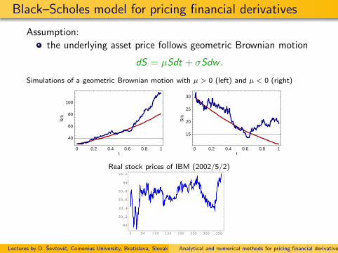
Assumption:
the underlying asset price follows geometric Brownian motion
dS = µSdt + σSdw .
Simulations of a geometric Brownian motion with µ > 0 (left) and µ < 0 (right)
0 0.2 0.4 0.6 0.8 1t
40
60
80
100
SHtL
0 0.2 0.4 0.6 0.8 1t
15
20
25
30
SHtL
Real stock prices of IBM (2002/5/2)
0 50 100 150 200 250 300 350
83
83.2
83.4
83.6
83.8
84
84.2
Lectures by D. Sevcovic, Comenius University, Bratislava, Slovak republicAnalytical and numerical methods for pricing financial derivatives

Black–Scholes model for pricing financial derivatives
A financial portfolio consisting of stocks (underlying assets),options and bonds
The aim is to dynamically (in time) rebalance the portfolio bybuying/selling stocks/options/bonds in order to reducevolatile fluctuations and to preserve its value
Lectures by D. Sevcovic, Comenius University, Bratislava, Slovak republicAnalytical and numerical methods for pricing financial derivatives

Black–Scholes model for pricing financial derivatives
Assumption:
Fundamental economic balances:
conservation of the total value of the portfolio
S QS + V QV + B = 0
requirement of self-financing the portfolio
S dQS + V dQV + δB = 0
QS is # of underlying assets with a unit price S in theportfolioQV is # of financial derivatives (options) with a unit price V
B the cash money in the portfolio (e.g. bonds, T-bills, etc.)
dQS is the change in the number of assetsdQV is the change in the number of optionsδB is the change in the cash due to buying/selling assets and options
Lectures by D. Sevcovic, Comenius University, Bratislava, Slovak republicAnalytical and numerical methods for pricing financial derivatives

Black–Scholes model for pricing financial derivatives
Assumption:
Secure bonds are appreciated by the fixed interest rate r > 0
B(t) = B(0)ert → dB = rB dt
The change of the total value of bonds in the portfolio istherefore
dB = rB dt + δB
because we sell bonds (δB < 0) or buy bonds (δB > 0) whenhedging (re-balancing) the portfolio in the time period[t, t + dt].
Lectures by D. Sevcovic, Comenius University, Bratislava, Slovak republicAnalytical and numerical methods for pricing financial derivatives

Black–Scholes model for pricing financial derivatives
Differentiating the fundamental balance law:S QS + V QV + B = 0 in the time period [t, t + dt] we obtain
0 = d (SQS + VQV + B) = d (SQS + VQV ) +
rB dt+δB︷ ︸︸ ︷
dB
0 =
=0︷ ︸︸ ︷
SdQS + VdQV + δB +QSdS + QV dV + rB dt
0 = QSdS + QVdV
rB︷ ︸︸ ︷
− r(SQS + VQV ) dt.
Dividing the last equation by QV we obtain
dV − rV dt −∆(dS − rS dt) = 0 , where ∆ = −QS
QV
.
Lectures by D. Sevcovic, Comenius University, Bratislava, Slovak republicAnalytical and numerical methods for pricing financial derivatives

Black–Scholes model for pricing financial derivatives
ReCall that we have assumed the stock price S to follow thegeometric Brownian motion
dS = µSdt + σSdw .
By Ito’s lemma we obtain for a smooth function V = V (S , t)
dV =
(∂V
∂t+
1
2σ2S2∂
2V
∂S2
)
dt +∂V
∂SdS .
Inserting the differential dV into the equationdV − rV dt −∆(dS − rS dt) = 0 we obtain
(∂V
∂t+
1
2σ2S2∂
2V
∂S2− rV +∆rS
)
dt +
(∂V
∂S−∆
)
dS = 0
Lectures by D. Sevcovic, Comenius University, Bratislava, Slovak republicAnalytical and numerical methods for pricing financial derivatives
Black–Scholes model for pricing financial derivatives
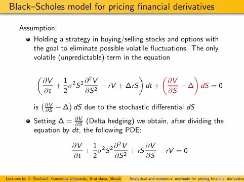
Assumption:
Holding a strategy in buying/selling stocks and options withthe goal to eliminate possible volatile fluctuations. The onlyvolatile (unpredictable) term in the equation
(∂V
∂t+
1
2σ2S2∂
2V
∂S2− rV +∆rS
)
dt +
(∂V
∂S−∆
)
dS = 0
is(∂V∂S −∆
)dS due to the stochastic differential dS
Setting ∆ = ∂V∂S (Delta hedging) we obtain, after dividing the
equation by dt, the following PDE:
∂V
∂t+
1
2σ2S2∂
2V
∂S2+ rS
∂V
∂S− rV = 0
Lectures by D. Sevcovic, Comenius University, Bratislava, Slovak republicAnalytical and numerical methods for pricing financial derivatives
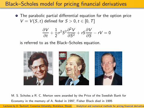
Black–Scholes model for pricing financial derivatives
The parabolic partial differential equation for the option priceV = V (S , t) defined for S > 0, t ∈ [0,T ]
∂V
∂t+
1
2σ2S2∂
2V
∂S2+ rS
∂V
∂S− rV = 0
is referred to as the Black–Scholes equation.
M. S. Scholes a R. C. Merton were awarded by the Price of the Swedish Bank for
Economy in the memory of A. Nobel in 1997, Fisher Black died in 1995
Lectures by D. Sevcovic, Comenius University, Bratislava, Slovak republicAnalytical and numerical methods for pricing financial derivatives

Black–Scholes model for pricing financial derivatives
Terminal conditions for the Black–Scholes equation:
At the time t = T of maturity (expiration) the price of a Calloption is easy to determine.
If the actual (spot) price S of the underlying asset at t = T isbigger then the exercise price E then it is worse to exercise theoption, and the holder should price this option by thedifference V (S ,T ) = S − E
If the actual (spot) price S of underlying asset at t = T is lessthen the exercise price E then the Call option has no value, i.e.V (S ,T ) = 0In both cases V (S ,T ) = max(S − E , 0).
0 20 40 60 80 100S
0
10
20
30
40
50
V
Lectures by D. Sevcovic, Comenius University, Bratislava, Slovak republicAnalytical and numerical methods for pricing financial derivatives

Black–Scholes model for pricing financial derivatives
Mathematical formulation of the problem of pricing a Call option:
Find a solution V (S , t) of the Black–Scholes parabolic partialdifferential equation
∂V
∂t+
1
2σ2S2∂
2V
∂S2+ rS
∂V
∂S− rV = 0
defined for S > 0, t ∈ [0,T ], and satisfying the terminalcondition
V (S ,T ) = max(S − E , 0)
at the time of maturity t = T .
Lectures by D. Sevcovic, Comenius University, Bratislava, Slovak republicAnalytical and numerical methods for pricing financial derivatives

Black–Scholes model for pricing financial derivatives
Solution of the Black–Scholes equation.
Using transformations x = ln(S/E ) and τ = T − t transformthe BS equation into the Cauchy problem
∂u
∂τ− σ2
2
∂2u
∂x2= 0,
u(x , 0) = u0(x),
for −∞ < x <∞ , τ ∈ [0,T ].
Solve this parabolic equation by means of the Green’s function
Transform back the solution and express V (S , t) in theoriginal variables S and t
Lectures by D. Sevcovic, Comenius University, Bratislava, Slovak republicAnalytical and numerical methods for pricing financial derivatives
Black–Scholes model for pricing financial derivatives
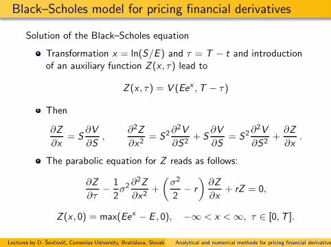
Solution of the Black–Scholes equation
Transformation x = ln(S/E ) and τ = T − t and introductionof an auxiliary function Z (x , τ) lead to
Z (x , τ) = V (Eex ,T − τ)
Then
∂Z
∂x= S
∂V
∂S,
∂2Z
∂x2= S2∂
2V
∂S2+ S
∂V
∂S= S2∂
2V
∂S2+∂Z
∂x.
The parabolic equation for Z reads as follows:
∂Z
∂τ− 1
2σ2∂2Z
∂x2+
(σ2
2− r
)∂Z
∂x+ rZ = 0,
Z (x , 0) = max(Eex − E , 0), −∞ < x <∞, τ ∈ [0,T ].
Lectures by D. Sevcovic, Comenius University, Bratislava, Slovak republicAnalytical and numerical methods for pricing financial derivatives

Black–Scholes model for pricing financial derivatives
Solution of the Black–Scholes equation
Using a new function u(x , τ)
u(x , τ) = eαx+βτZ (x , τ)
where α, β ∈ R are some constants leads to
∂u
∂τ− σ2
2
∂2u
∂x2+ A
∂u
∂x+ Bu = 0 ,
u(x , 0) = Eeαx max(ex − 1, 0),
Constants
A = ασ2 +σ2
2− r , and B = (1 + α)r − β − α2σ2 + ασ2
2.
can be eliminated (i.e. A = 0,B = 0) by setting
α =r
σ2− 1
2, β =
r
2+σ2
8+
r2
2σ2.
Lectures by D. Sevcovic, Comenius University, Bratislava, Slovak republicAnalytical and numerical methods for pricing financial derivatives

Black–Scholes model for pricing financial derivatives
Solution of the Black–Scholes equation
A solution u(x , τ) to the Cauchy problem ∂u∂τ − σ2
2∂2u∂x2
= 0 isgiven by Green’s formula
u(x , τ) =1√
2σ2πτ
∫ ∞
−∞e− (x−s)2
2σ2τ u(s, 0) ds .
Computing this integral and transforming back to the originalvariables S , t and V (S , t), enables us to conclude
V (S , t) = SN(d1)− Ee−r(T−t)N(d2) ,
where N(x) = 1√2π
∫ x
−∞ e−ξ2
2 dξ is a distribution function of
the normal distribution and
d1 =ln S
E+ (r + σ2
2 )(T − t)
σ√T − t
, d2 = d1 − σ√T − t
Lectures by D. Sevcovic, Comenius University, Bratislava, Slovak republicAnalytical and numerical methods for pricing financial derivatives

Black–Scholes model for pricing financial derivatives
Solution of the Black–Scholes equation
45 50 55 60 65 70 75S
2
4
6
8
10
12
14
V
45 50 55 60 65 70 75S
2
4
6
8
10
12
14
V
Graph of a solution V (S, 0) for a Call option together with the terminal condition
V (S,T ) (left). Graphs of solutions V (S, t) for different times T − t to maturity
(right).
Example:Present (spot) price of the IBM stock is S = 58.5 USDHistorical volatility of the stock price was estimated to σ = 29% p.a., i.e.σ = 0.29.Interest rate for secure bonds r = 4% p.a., i.e. r = 0.04Call option for the exercise price E = 60 USD and exercise time T = 0.3-yearsComputed Call option price by Black–Scholes formula is:V=V(58.5, 0) = 3.35 USD.Real market price was V = 3.4 USD
Lectures by D. Sevcovic, Comenius University, Bratislava, Slovak republicAnalytical and numerical methods for pricing financial derivatives

Black–Scholes model for pricing financial derivatives
Put option
Put option is an agreement (contract) between the writer(issuer) and the holder of an option. It represents the rightBUT NOT the obligation to SELL the underlying asset at theprescribed exercise price E at the specified time of maturityt = T in the future.
If the actual (spot) price S of the underlying asset at t = T isless then the exercise price E then it is worse to exercise theoption, and the holder prices this option as the differenceV (S ,T ) = E − S .
If the actual (spot) price S of underlying asset at t = T ishigher then the exercise price E then it has no value for theholder, i.e. V (S ,T ) = 0.
In both cases we have V (S ,T ) = max(E − S , 0).
Lectures by D. Sevcovic, Comenius University, Bratislava, Slovak republicAnalytical and numerical methods for pricing financial derivatives

Black–Scholes model for pricing financial derivatives
Put option
explicit solution to the Black-Scholes equation with theterminal condition V (S ,T ) = max(E − S , 0)
Vep(S , t) = Ee−r(T−t)N(−d2)− SN(−d1)
where N(.), d1, d2 are defined as in the case of a Call option.
50 55 60 65 70 75S
2
4
6
8
10
12
V
50 55 60 65 70 75S
2
4
6
8
10
12
V
Graph of a solution V (S, 0) for a Put option and the terminal condition V (S,T )
(left). Graphs of solutions V (S, t) for different times T − t to maturity (right)
Lectures by D. Sevcovic, Comenius University, Bratislava, Slovak republicAnalytical and numerical methods for pricing financial derivatives

Black–Scholes model for pricing financial derivatives
Put-Call parity
Construct a portfolio of one long Call option and one shortPut option: Vf (S ,T ) = Vec(S ,T ) − Vep(S ,T )
Vf (S ,T ) = max(S − E , 0) −max(E − S , 0) = S − E .
The solution to the Black–Scholes equation with the terminalcondition Vf (S ,T ) = S − E can be found easily
Vf (S , t) = S − Ee−r(T−t)
According to the linearity of the Black–Scholes equation weobtain:
Vec(S , t)− Vep(S , t) = S − Ee−r(T−t)
known as the Put–Call parity: Call - Put = Asset - Forward
Lectures by D. Sevcovic, Comenius University, Bratislava, Slovak republicAnalytical and numerical methods for pricing financial derivatives

Selected option strategies
Bullish spreadBuy one Call option on the exercise price E1 and sell one Calloption on E2 where E1 < E2. Therefore the Pay–off diagram:V (S ,T ) = max(S − E1, 0) − max(S − E2, 0)
0 20 40 60 80 100S
-10
-5
0
5
10
V
0 20 40 60 80 100S
-10
-5
0
5
10
V
The strategy has a limited profit and limited loss (pay-offdiagram is bounded).It protects the holder for increase of the asset price in a shortposition (like a single Call option).Linearity of the Black–Scholes equation implies:
V (S , t) = V c(S , t;E1)− V c(S , t;E2), for all 0 ≤ t ≤ T
Lectures by D. Sevcovic, Comenius University, Bratislava, Slovak republicAnalytical and numerical methods for pricing financial derivatives
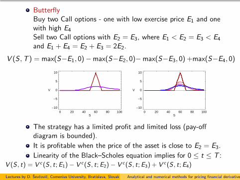
ButterflyBuy two Call options - one with low exercise price E1 and onewith high E4
Sell two Call options with E2 = E3, where E1 < E2 = E3 < E4
and E1 + E4 = E2 + E3 = 2E2.
V (S ,T ) = max(S−E1, 0)−max(S−E2, 0)−max(S−E3, 0) +max(S−E4, 0)
0 20 40 60 80 100S
-10
-5
0
5
10
V
0 20 40 60 80 100S
-10
-5
0
5
10
V
The strategy has a limited profit and limited loss (pay-offdiagram is bounded).
It is profitable when the price of the asset is close to E2 = E3.
Linearity of the Black–Scholes equation implies for 0 ≤ t ≤ T :V (S , t) = V c (S , t;E1)− V c(S , t;E2)− V c(S , t;E3) + V c (S , t;E4)
Lectures by D. Sevcovic, Comenius University, Bratislava, Slovak republicAnalytical and numerical methods for pricing financial derivatives

Strangle is a combination of purchasing one Call on E2, andone Put option on strike price E1 < E2
V (S ,T ) = (S − E2)+ + (E1 − S)+ .
Condor is a strategy similar to butterfly, but the difference isthat the strike prices of sold Call options need not be equal,E2 6= E3, i.e., E1 < E2 < E3 < E4.
30 40 50 60 70 80 90 100S
10
20
30
40
50
V
0 20 40 60 80 100S
0
2
4
6
8
10
V
Left: Strangle option strategy for E1 = 50;E2 = 70 and pricesS 7→ V (S , t)
Right: Condor option strategy with E1 = 50,E2 = 60,E3 = 65,E4 = 70
Lectures by D. Sevcovic, Comenius University, Bratislava, Slovak republicAnalytical and numerical methods for pricing financial derivatives

Black–Scholes equation for divedend paying assets
the underlying asset is paying nontrivial continuous dividendswith an annualized dividend yield D ≥ 0holder of the underlying asset receives a dividend yield DSdt
over any time interval with a length dt
paying dividends leads to the asset price decrease
dS = (µ − D)S dt + σSdw .
on the other hand, it is added as an extra income to themoney volume of secure bonds
dB = rB dt + δB + DSQS dt
the portfolio balance equation then becomes
QV dV + QSdS + rB dt + DSQS dt = 0
since B = −QVV − QSS we obtain, after dividing by QV ,
dV −rV dt−∆(dS−(r−D)S dt) = 0 where ∆ = −QS/QV .
Lectures by D. Sevcovic, Comenius University, Bratislava, Slovak republicAnalytical and numerical methods for pricing financial derivatives

repeating steps of derivation of the B-S equation, using Ito’slemma for dV we conclude with the equation
∂V
∂t+
1
2σ2S2 ∂
2V
∂S2+ (r − D)S
∂V
∂S− rV = 0
similarly as in the case D = 0 we obtain
V (S , t) = Se−D(T−t)N(d1)− Ee−r(T−t)N(d2) ,
d1 =ln S
E+ (r − D + σ2
2 )(T − t)
σ√T − t
, d2 = d1 − σ√T − t
Put option can be calculated from Put-Call parity:V c(S , t)− V p(S , t) = Se−D(T−t) − Ee−r(T−t)
50 60 70 80 90 100 110 120S
0
10
20
30
40
V
0 20 40 60 80 100 120S
0
20
40
60
80
V
Solutions V (S, t), 0 ≤ t < T , for a European Call option (left) and Put option (right).
Lectures by D. Sevcovic, Comenius University, Bratislava, Slovak republicAnalytical and numerical methods for pricing financial derivatives

Finite difference method for solving the Black–Scholesequation
Lecture 4
Transformation of the Black–Scholes equation to the heatequation
Finite difference approximation
Explicit numerical scheme and the method of binomial trees
Stable implicit numerical scheme using a linear algebra solver
Lectures by D. Sevcovic, Comenius University, Bratislava, Slovak republicAnalytical and numerical methods for pricing financial derivatives

Numerical solution to the Black–Scholes equation
using the transformation V (S , t) = Ee−αx−βτu(x , τ), whereτ = T − t, x = ln(S/E ), leads to the heat equation
∂u
∂τ− σ2
2
∂2u
∂x2= 0
for any x ∈ R, 0 < τ < T .
g(x , τ) =
eαx+βτ max(ex − 1, 0), for a Call option,eαx+βτ max(1− ex , 0), for a Put option.
represents the transformed pay-off diagram of a Call (Put)option
It satisfies the initial condition
u(x , 0) = g(x , 0), for any x ∈ R.
Here: α = r−Dσ2 − 1
2, β = r+D
2+ σ2
8+
(r−D)2
2σ2
Lectures by D. Sevcovic, Comenius University, Bratislava, Slovak republicAnalytical and numerical methods for pricing financial derivatives

Finite difference approximation of a solution u(x , τ)
spatial and time discretization yields the finite difference mesh
xi = ih, i = ...,−2,−1, 0, 1, 2, ..., τj = jk , j = 0, 1, ...,m.
h = L/n, k = T/m.
approximation of the solution u at (xi , τj) will be denoted by
uji ≈ u(xi , τj ), and also g
ji ≈ g(xi , τj)
using boundary conditionsCall option: V (0, t) = 0 and V (S , t)/S → e−D(T−t) for S → ∞Put option: V (0, t) = Ee−r(T−t) and V (S , t) → 0 as S → ∞⇒ the boundary condition at x = ±L, L ≫ 1,
uj−N = φj :=
0, for a European Call option,
e−αNh+(β−r)jk , for a European Put option,
ujN = ψj :=
e(α+1)Nh+(β−D)jk , for a European Call option,0, for a European Put option.
Lectures by D. Sevcovic, Comenius University, Bratislava, Slovak republicAnalytical and numerical methods for pricing financial derivatives

time derivative forward (explicit) and backward (implicit)finite difference approximation
∂u
∂τ(xi , τj) ≈
uj+1i − u
ji
k︸ ︷︷ ︸
forward
∂u
∂τ(xi , τj) ≈
uji − u
j−1i
k︸ ︷︷ ︸
backward
central finite difference approximation of the spatial derivative
∂2u
∂x2(xi , τj) ≈
uji+1 − 2uji + u
ji−1
h2
Explicit and implicit finite difference approximation of theheat equation
uj+1i − u
ji
k=σ2
2
uji+1 − 2uji + u
ji−1
h2︸ ︷︷ ︸
explicit scheme
,uji − u
j−1i
k=σ2
2
uji+1 − 2uji + u
ji−1
h2︸ ︷︷ ︸
implicit scheme
Lectures by D. Sevcovic, Comenius University, Bratislava, Slovak republicAnalytical and numerical methods for pricing financial derivatives
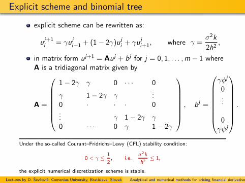
Explicit scheme and binomial tree
explicit scheme can be rewritten as:
uj+1i = γuji−1 + (1− 2γ)uji + γuji+1, where γ =
σ2k
2h2,
in matrix form uj+1 = Auj + bj for j = 0, 1, . . . ,m − 1 whereA is a tridiagonal matrix given by
A =
1− 2γ γ 0 · · · 0
γ 1− 2γ γ...
0 · · · 0... γ 1− 2γ γ0 · · · 0 γ 1− 2γ
, bj =
γφj
0...
0γψj
.
Under the so-called Courant–Fridrichs–Lewy (CFL) stability condition:
0 < γ ≤ 1
2, i.e.
σ2k
h2≤ 1,
the explicit numerical discretization scheme is stable.
Lectures by D. Sevcovic, Comenius University, Bratislava, Slovak republicAnalytical and numerical methods for pricing financial derivatives

Explicit scheme and numerical oscillations
transforming back to the original variablesS = Eex , t = T − τ,V (S , t) = Ee−αx−βτu(x , τ) we obtainthe option price V
30 40 50 60 70S
0
5
10
15
20
V
30 40 50 60 70S
0
5
10
15
20
V
A solution S 7→ V (S , t) for the price of a European Call option
obtained by means of the binomial tree method with γ = 1/2 (left)
and comparison with the exact solution (dots). The oscillating
solution S 7→ V (S , t) which does not converge to the exact solution
for the parameter value γ = 0.56 > 1/2, where γ > 1/2, does not
fulfill the CFL condition.
Lectures by D. Sevcovic, Comenius University, Bratislava, Slovak republicAnalytical and numerical methods for pricing financial derivatives

Explicit numerical scheme and binomial tree
if we choose the ratio between the spatial and timediscretization steps such that h = σ
√k then γ = 1/2
uj+1i =
1
2uji−1 +
1
2uji+1.
the solution uj+1i at the time τj+1 is the arithmetic average
between values uji−1 and uji+1
A binomial tree as an illustration of the algorithm for solving a
parabolic equation by an explicit method with 2γ = σ2k/h2 = 1.
Lectures by D. Sevcovic, Comenius University, Bratislava, Slovak republicAnalytical and numerical methods for pricing financial derivatives

Explicit numerical scheme and binomial tree
The binomial pricing model can be also derived from the explicitnumerical scheme.
Vji ≈ V (Si ,T − τj), where Si = Eexi = Ee ih.
since V (S , t) = Ee−αx−βτu(x , t), we obtainV
ji = Ee−αih−βjkuji .
in terms of the original variable Vji , the explicit numerical
scheme can be expressed as follows:
Vj+1i = e−rk
(
q−Vji−1 + q+V
ji+1
)
, where q± =1
2e±αh−(β−r)k .
for k → 0 and h = σ√k → 0 we have
q+.=
1 + αh
2, q−
.=
1− αh
2, q− + q+ = 1.
and these constants are refereed to as risk-neutralprobabilities.
Lectures by D. Sevcovic, Comenius University, Bratislava, Slovak republicAnalytical and numerical methods for pricing financial derivatives
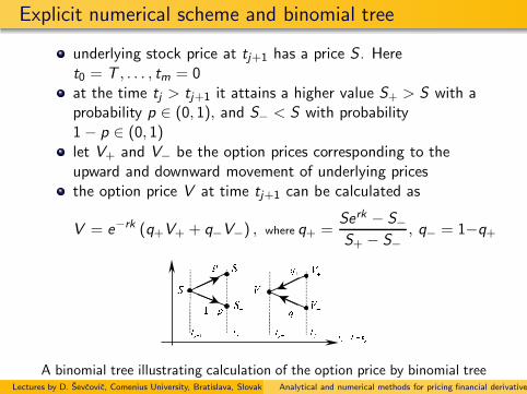
Explicit numerical scheme and binomial tree
underlying stock price at tj+1 has a price S . Heret0 = T , . . . , tm = 0at the time tj > tj+1 it attains a higher value S+ > S with aprobability p ∈ (0, 1), and S− < S with probability1− p ∈ (0, 1)let V+ and V− be the option prices corresponding to theupward and downward movement of underlying pricesthe option price V at time tj+1 can be calculated as
V = e−rk (q+V+ + q−V−) , where q+ =Serk − S−S+ − S−
, q− = 1−q+
A binomial tree illustrating calculation of the option price by binomial treeLectures by D. Sevcovic, Comenius University, Bratislava, Slovak republicAnalytical and numerical methods for pricing financial derivatives
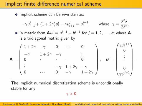
Implicit finite difference numerical scheme
implicit scheme can be rewritten as:
−γuji−1 + (1 + 2γ)uji − γuji+1 = uj−1i , where γ =
σ2k
2h2,
in matrix form Auj = uj−1 + bj−1 for j = 1, 2, . . . ,m where A
is a tridiagonal matrix given by
A =
1 + 2γ −γ 0 · · · 0
−γ 1 + 2γ −γ ...0 · · · 0... −γ 1 + 2γ −γ0 · · · 0 −γ 1 + 2γ
, bj =
γφj+1
0...
0γψj+1
.
The implicit numerical discretization scheme is unconditionallystable for any
γ > 0
Lectures by D. Sevcovic, Comenius University, Bratislava, Slovak republicAnalytical and numerical methods for pricing financial derivatives

Implicit finite difference numerical scheme
transforming back to the original variablesS = Eex , t = T − τ,V (S , t) = Ee−αx−βτu(x , τ) we obtainthe option price V
30 40 50 60 70S
0
5
10
15
20
V
30 40 50 60 70S
0
5
10
15
20
V
A solution S 7→ V (S , t) for pricing a European Call option obtained by
means of the implicit finite difference method with γ = 1/2 (left) and
comparison with the exact analytic solution (dots). The numerical
scheme is also stable for a large value of the parameter γ = 20 > 1/2 not
satisfying the CFL condition (right).
Lectures by D. Sevcovic, Comenius University, Bratislava, Slovak republicAnalytical and numerical methods for pricing financial derivatives

How we solve linear algebra problem
Successive Over Relaxation method for solving Au = b
Decompose the matrix A as as sum of subdiagonal, diagonal and overdiagonalmatrix A = L+ D+ U where
Lij = Aij for j < i , otherwise Lij = 0,
Dij = Aij for j = i , otherwise Dij = 0,
Uij = Aij for j > i , otherwise Uij = 0.
We suppose that D is invertible. Let ω > 0 be a relaxation parameter. Asolution of Au = b is equivalent to
Du = Du + ω(b − Au).
or, equivalently,(D+ ωL)u = (1 − ω)Du + ω(c − Uu).
Therefore u is a solution of
u = Tωu + cω , where Tω = (D+ ωL)−1 ((1 − ω)D− ωU)
a cω = ω(D+ ωL)−1b.
Define a recurrent sequence of approximate solution
u0 = 0, up+1 = Tωup + cω for p = 1, 2, ...
Lectures by D. Sevcovic, Comenius University, Bratislava, Slovak republicAnalytical and numerical methods for pricing financial derivatives

the SOR algorithm reduces to successive calculation, forp = 0, ..., pmax of
up+1i =
ω
Aii
bi −∑
j<i
Aijup+1j −
∑
j>i
Aijupj
+ (1− ω)upi
for i = 1, ...,N
where ω ∈ (1, 2) is a relaxation parameter
if ‖Tω‖ < 1 then the mapping Rn ∋ u 7→ Tωu + cω ∈ R
n iscontractive and the fixed point argument implies that up
converges to u for p → ∞ and Au = b.
0.8 1 1.2 1.4 1.6 1.8 2 2.2Ω
0.6
0.8
1
1.2
ÈTΩÈ
Graph of the spectral norm of the iteration operator ‖Tω‖ as a function of the
relaxation parameter ω.
Lectures by D. Sevcovic, Comenius University, Bratislava, Slovak republicAnalytical and numerical methods for pricing financial derivatives

Black–Scholes model and sensitivity analysis
Lecture 5
Historical and implied volatilities
Computation of the implied volatility
Sensitivity with respect to model parameters
Delta and Gamma of an option. Other Greeks factors.
Lectures by D. Sevcovic, Comenius University, Bratislava, Slovak republicAnalytical and numerical methods for pricing financial derivatives
Black–Scholes model and sensitivity analysis
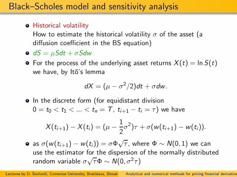
Historical volatilityHow to estimate the historical volatility σ of the asset (adiffusion coefficient in the BS equation)
dS = µSdt + σSdw
For the process of the underlying asset returns X (t) = lnS(t)we have, by Ito’s lemma
dX = (µ− σ2/2)dt + σdw .
In the discrete form (for equidistant division0 = t0 < t1 < ... < tn = T , ti+1 − ti = τ) we have
X (ti+1)− X (ti) = (µ− 1
2σ2)τ + σ(w(ti+1)− w(ti )).
as σ(w(ti+1)− w(ti)) = σΦ√τ , where Φ ∼ N(0, 1) we can
use the estimator for the dispersion of the normally distributedrandom variable σ
√τΦ ∼ N(0, σ2τ)
Lectures by D. Sevcovic, Comenius University, Bratislava, Slovak republicAnalytical and numerical methods for pricing financial derivatives

Black–Scholes model and sensitivity analysis
The historical volatility σ = σhist of the underlying asset price
σ2hist =1
τ
1
n− 1
n−1∑
i=0
(
ln(S(ti+1)/S(ti ))− γ)2
where γ is the mean value of returnsX (ti ) = ln(S(ti+1)/S(ti ))
γ =1
n
n−1∑
i=0
ln(S(ti+1)/S(ti )).
0 50 100 150 200 250 300 350t
83.8
84
84.2
84.4
84.6
84.8
S
IBM stock price evolution from 21.5.2002 with τ = 1 minute. The computed
historical volatility σhist = 0.2306 on the yearly basis, i.e. σhist = 23% p.a.
Lectures by D. Sevcovic, Comenius University, Bratislava, Slovak republicAnalytical and numerical methods for pricing financial derivatives

Black–Scholes model and sensitivity analysis
0 50 100 150 200 250 300 350t
6.6
6.8
7
7.2
V
IBM Call option price from 21.5.2002 (red).
Computed V ec(Sreal (t), t; σhist) with σhist = 0.2306 (blue)
In typical real market situations the historical volatility σhistproduces lower option prices
σhist is lower than the value that is needed for exact matchingof market option prices
Lectures by D. Sevcovic, Comenius University, Bratislava, Slovak republicAnalytical and numerical methods for pricing financial derivatives
Black–Scholes model and sensitivity analysis
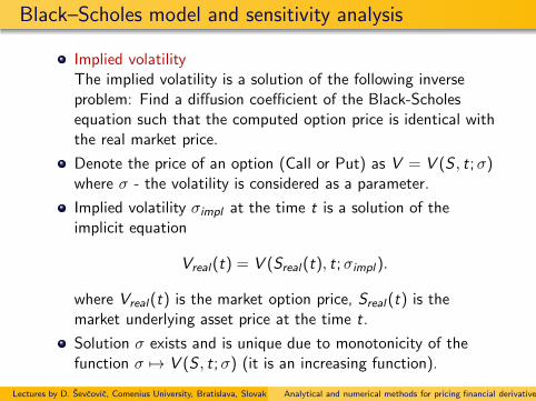
Implied volatilityThe implied volatility is a solution of the following inverseproblem: Find a diffusion coefficient of the Black-Scholesequation such that the computed option price is identical withthe real market price.
Denote the price of an option (Call or Put) as V = V (S , t;σ)where σ - the volatility is considered as a parameter.
Implied volatility σimpl at the time t is a solution of theimplicit equation
Vreal(t) = V (Sreal(t), t;σimpl ).
where Vreal(t) is the market option price, Sreal (t) is themarket underlying asset price at the time t.
Solution σ exists and is unique due to monotonicity of thefunction σ 7→ V (S , t;σ) (it is an increasing function).
Lectures by D. Sevcovic, Comenius University, Bratislava, Slovak republicAnalytical and numerical methods for pricing financial derivatives
Black–Scholes model and sensitivity analysis
0 50 100 150 200 250 300 350t
83.8
84
84.2
84.4
84.6
84.8
S
0 50 100 150 200 250 300 350t
6.6
6.8
7
7.2
V
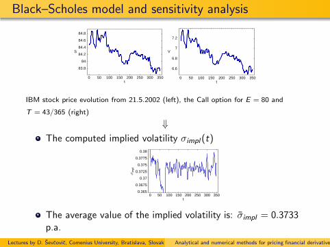
IBM stock price evolution from 21.5.2002 (left), the Call option for E = 80 and
T = 43/365 (right)
⇓The computed implied volatility σimpl (t)
0 50 100 150 200 250 300 350t
0.365
0.3675
0.37
0.3725
0.375
0.3775
0.38
Σim
pl
The average value of the implied volatility is: σimpl = 0.3733p.a.
Lectures by D. Sevcovic, Comenius University, Bratislava, Slovak republicAnalytical and numerical methods for pricing financial derivatives
Black–Scholes model and sensitivity analysis
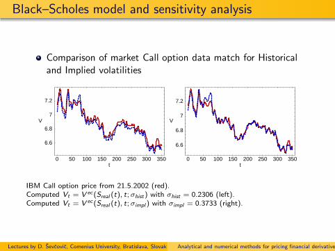
Comparison of market Call option data match for Historicaland Implied volatilities
0 50 100 150 200 250 300 350t
6.6
6.8
7
7.2
V
0 50 100 150 200 250 300 350t
6.6
6.8
7
7.2
V
IBM Call option price from 21.5.2002 (red).Computed Vt = V ec(Sreal (t), t; σhist) with σhist = 0.2306 (left).Computed Vt = V ec(Sreal (t), t; σimpl ) with σimpl = 0.3733 (right).
Lectures by D. Sevcovic, Comenius University, Bratislava, Slovak republicAnalytical and numerical methods for pricing financial derivatives

Black–Scholes model and sensitivity analysis
Sensitivity of the option price with respect to model parameters -Greeks
Sensitivity with respect to the asset price: Delta - ∆,
∆ =∂V
∂S
It measures the rate of change of the option price V w.r. tothe change in the asset price S
It is used in the so-called Delta hedging because therisk-neutral portfolio is balanced according to the law:
QS
QV
= −∂V∂S
= −∆
where QV , QS is the number of options and stocks in theportfolio
Lectures by D. Sevcovic, Comenius University, Bratislava, Slovak republicAnalytical and numerical methods for pricing financial derivatives

Black–Scholes model and sensitivity analysis
Delta for European Call and Put options:
∆ec =∂V ec
∂S= N(d1), ∆ep =
∂V ep
∂S= −N(−d1).
50 60 70 80 90 100S
0
0.2
0.4
0.6
0.8
D
50 60 70 80 90 100S
-1
-0.8
-0.6
-0.4
-0.2
D
∆ec ∆ep
Parameters: E = 80, r = 0.04,T = 43/365
Notice that ∆ec ∈ (0, 1) and ∆ep ∈ (−1, 0)
Lectures by D. Sevcovic, Comenius University, Bratislava, Slovak republicAnalytical and numerical methods for pricing financial derivatives

Black–Scholes model and sensitivity analysis
Computation of Delta for market data time series
Determine the implied volatility σimpl(t) from market datatime series of the option price Vreal(t) and the underlyingasset price Sreal(t). We solve
Vreal(t) = V ec(Sreal(t), t;σimpl (t)).
Produce the graph of ∆ec(t) = ∂V ec
∂S (Sreal (t), t;σimpl (t))
0 50 100 150 200 250 300 350t
0.68
0.69
0.7
0.71
D
Observe that the decrease of Delta means that keeping oneCall option we have to decrease the number QS of owedstocks in the portfolio.
Lectures by D. Sevcovic, Comenius University, Bratislava, Slovak republicAnalytical and numerical methods for pricing financial derivatives
Black–Scholes model and sensitivity analysis
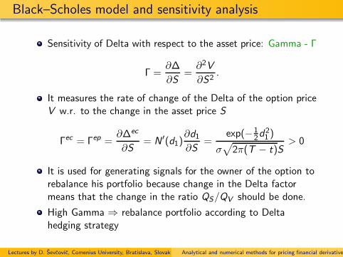
Sensitivity of Delta with respect to the asset price: Gamma - Γ
Γ =∂∆
∂S=∂2V
∂S2.
It measures the rate of change of the Delta of the option priceV w.r. to the change in the asset price S
Γec = Γep =∂∆ec
∂S= N ′(d1)
∂d1∂S
=exp(−1
2d21 )
σ√
2π(T − t)S> 0
It is used for generating signals for the owner of the option torebalance his portfolio because change in the Delta factormeans that the change in the ratio QS/QV should be done.
High Gamma ⇒ rebalance portfolio according to Deltahedging strategy
Lectures by D. Sevcovic, Comenius University, Bratislava, Slovak republicAnalytical and numerical methods for pricing financial derivatives

Black–Scholes model and sensitivity analysis
Computation of Gamma for market data time seriesDetermine the implied volatility σimpl (t) from market data time series of theoption price Vreal (t) and the underlying asset price Sreal (t). We solve
Vreal (t) = V ec(Sreal (t), t;σimpl (t)).
Produce the graph of Γec (t) = ∂2V ec
∂S2 (Sreal (t), t; σimpl (t))
0 50 100 150 200 250 300 350t
83.8
84
84.2
84.4
84.6
84.8
S
0 50 100 150 200 250 300 350t
6.6
6.8
7
7.2
V
IBM stock price from 21.5.2002 (left), Call option for E = 80 and T = 43/365 (right)
0 50 100 150 200 250 300 350t
0.68
0.69
0.7
0.71
D
0 50 100 150 200 250 300 350t
0.0315
0.032
0.0325
0.033
0.0335
G
Delta (left)
Lectures by D. Sevcovic, Comenius University, Bratislava, Slovak republicAnalytical and numerical methods for pricing financial derivatives

Black–Scholes model and sensitivity analysis
Other Greeks - Sensitivity of the option price to model parameters
RhoSensitivity with respect to the interest rate r , P = ∂V
∂r
ThetaSensitivity with respect to time t, Θ = ∂V
∂t
VegaSensitivity with respect to volatility σ, Υ = ∂V
∂σ
Greek version of the Black–Scholes equation.
∂V
∂t+
1
2σ2S2∂
2V
∂S2+ rS
∂V
∂S− rV = 0
⇓
Θ+σ2
2S2Γ + rS∆− rV = 0
Lectures by D. Sevcovic, Comenius University, Bratislava, Slovak republicAnalytical and numerical methods for pricing financial derivatives

Exotic derivatives
Lecture 6
Path dependent options, concepts and applications
Barrier options, formulation in terms of a solution to a partialdifferential equation on a time dependent domain
Asian options, formulation in terms of a solution to a partialdifferential equation in a higher dimension
Numerical methods for solving barrier and Asian options
Lectures by D. Sevcovic, Comenius University, Bratislava, Slovak republicAnalytical and numerical methods for pricing financial derivatives

Exotic derivatives - Path dependent options
Path dependent options
A path-dependent option = the option contract depends onthe whole time evolution of the underlying asset in the timeinterval [0,T ]
Classical European options are not path dependent options,the contract depends only on the terminal pay-off V (S ,T ) atthe expiry T
The path dependent options - ExamplesBarrier options - the contract depends on whether the assetprice jumped over/under prescribed barrierAsian options - the contract depends on the average of theasset price over the time interval [0,T ]Many other like e.g. look-back options, Russian options, Israelioptions, etc.
Path dependent options are hard to price as the contractdepends on the whole evolution of the asset price St in thefuture time interval [0,T ]
Lectures by D. Sevcovic, Comenius University, Bratislava, Slovak republicAnalytical and numerical methods for pricing financial derivatives

Exotic derivatives - Barrier options
Example of an barrier options: Down–and–out Call option.This is a usual Call option with the terminal pay-offV (S ,T ) = max(S − E , 0) except of the fact that the optionmay expire before the maturity T at the time t < T in thecase when the underlying asset price St reaches the prescribedbarrier B(t) from above.
0 0.2 0.4 0.6 0.8 1t
30
40
50
60
70
S
0 0.2 0.4 0.6 0.8 1t
30
40
50
60
70
S
opcia expirovala
The option will expire at the maturity T (left) It will expire prematurely at t < T (right)
If the option expires prematurely at t < T the writer pays theholder the prescribed rabat R(t).
Lectures by D. Sevcovic, Comenius University, Bratislava, Slovak republicAnalytical and numerical methods for pricing financial derivatives

Exotic derivatives - Barrier options
A typical exponential barrier function is: B(t) = bEe−α(T−t)
with 0 < b < 1
A typical exponential rabat function is:R(t) = E
(1− e−β(T−t)
)
Mathematical formulation - the PDE on a time dependentdomain
∂V
∂t+
1
2σ2S2∂
2V
∂S2+ rS
∂V
∂S− rV = 0
for t ∈ [0,T ) and B(t) < S <∞
V (B(t), t) = R(t), t ∈ [0,T )
at the left barrier boundary S = B(t)
V (S ,T ) = max(S − E , 0), S > 0,
at t = T (Barrier Call option).
Lectures by D. Sevcovic, Comenius University, Bratislava, Slovak republicAnalytical and numerical methods for pricing financial derivatives

Exotic derivatives - Barrier options
The fixed domain transformation
V (S , t) = W (x , t), where x = ln (S/B(t)) , x ∈ (0,∞),
transforms the problem from the time dependent domainB(t) < S <∞ to the fixed domain x ∈ (0,∞).For an exponential barrier function B(t) = bEe−α(T−t) wehave B(t) = αB(t).After performing necessary substitutions we obtain the PDEfor the transformed function W (x , t)
∂W
∂t+σ2
2
∂2W
∂x2+
(
r − σ2
2− α
)∂W
∂x− rW = 0.
The terminal condition for the Call option case:
W (x ,T ) = E max(bex − 1, 0).
The left side boundary condition
W (0, t) = R(t).
Lectures by D. Sevcovic, Comenius University, Bratislava, Slovak republicAnalytical and numerical methods for pricing financial derivatives

Exotic derivatives - Barrier options
A numerical solution - a simple code in the software Mathematica
b = 0.7; alfa = 0.1; beta = 0.05; X = 40; sigma = 0.4; r = 0.04; d = 0; T = 1;
xmax = 2;
Bariera[t_] := X b Exp[-alfa (T - t)]; Rabat[t_] := X (1 - Exp[-beta(T - t)]);
PayOff[x_] := X*If[b Exp[x] - 1 > 0, b Exp[x] - 1, 0];
riesenie = NDSolve[
D[w[x, tau], tau] == (sigma^2/2)D[w[x, tau], x, x]
+ (r - d - sigma^2/2 - alfa )* D[w[x, tau], x]
- r *w[x, tau] ,
w[x, 0] == PayOff[x],
w[0, tau] == Rabat[T - tau],
w[xmax, tau] == PayOff[xmax],
w, tau, 0, T, x, 0, xmax
];
w[x_, tau_] := Evaluate[w[x, tau] /. riesenie[[1]] ];
Plot3D[w[x, tau], x, 0, xmax, tau, 0, T];
V[S_, tau_] :=
If[S > Bariera[T - tau],
w[ Log[S/Bariera[T - tau]], tau],
Rabat[T - tau]
];
Plot[ V(S,0.2 T],V(S,0.4 T], V(S,0.6 T], V(S,0.8 T], V(S,T], S,20,50];
Lectures by D. Sevcovic, Comenius University, Bratislava, Slovak republicAnalytical and numerical methods for pricing financial derivatives

Exotic derivatives - Barrier options
A numerical solution - an example of a solution to theDown-and-out barrier Call option
20 25 30 35 40 45S
0
2
4
6
8
10
12
V
Graph of the solution of the barrier Call option for different times t ∈ [0,T ]
Lectures by D. Sevcovic, Comenius University, Bratislava, Slovak republicAnalytical and numerical methods for pricing financial derivatives

Exotic derivatives - Asian options
An example of an Asian option:This is a Call option with terminal pay-offV (S ,T ) = max(S − E , 0) except of the fact that the exerciseprice E is not prescribed but it is given as the arithmetic (orgeometric) average of the underlying asset prices St withinthe time interval [0,T ], i.e. the terminal pay-off diagram is:
V (S ,T ) = max(S − AT , 0)
arithmetic average geometric average
At =1
t
∫ t
0Sτdτ, lnAt =
1
t
∫ t
0lnSτdτ.
In the discrete form
Atn =1
n
n∑
i=1
Sti , lnAtn =1
n
n∑
i=1
lnSti ,
where t1 < t2 < ... < tn, and ti+1 − ti = 1/n.Lectures by D. Sevcovic, Comenius University, Bratislava, Slovak republicAnalytical and numerical methods for pricing financial derivatives

Exotic derivatives - Asian options
0 0.1 0.2 0.3 0.4 0.5 0.6 0.7 0.8 0.9 119
20
21
22
23
24
25
26
27
28
29
S
A
A−X
Simulated price of the underlying asset and the corresponding arithmetic
average.
Lectures by D. Sevcovic, Comenius University, Bratislava, Slovak republicAnalytical and numerical methods for pricing financial derivatives

Exotic derivatives - Asian options
Assume the asset price follows SDE: dS = µSdt + σSdw
The average A is the arithmetic average, i.e. At =1t
∫ t
0 SτdτThen
dA
dt= − 1
t2
∫ t
0Sτdτ +
1
tSt =
St − At
t
an hence, in the differential form, dA = S−At
dt.
In general we may assume
dA = A f
(S
A, t
)
dt, f (x , t) =x − 1
t, f (x , t) =
ln x
t
general form arithmetic average geometric average
Construct the option price as a function
V = V (S ,A, t)
It depends on a new variable: A - the average of the assetprice
Lectures by D. Sevcovic, Comenius University, Bratislava, Slovak republicAnalytical and numerical methods for pricing financial derivatives
Exotic derivatives - Asian options
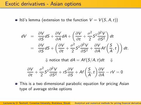
Ito’s lemma (extension to the function V = V (S ,A, t))
dV =∂V
∂SdS +
∂V
∂AdA+
(∂V
∂t+σ2
2S2∂
2V
∂S2
)
dt
=∂V
∂SdS +
(∂V
∂t+σ2
2S2∂
2V
∂S2+∂V
∂AAf
(S
A, t
))
dt.
⇓ notice that dA = Af (S/A, t)dt ⇓
∂V
∂t+σ2
2S2∂
2V
∂S2+ rS
∂V
∂S+ Af
(S
A, t
)∂V
∂A− rV = 0
This is a two dimensional parabolic equation for pricing Asiantype of average strike options
Lectures by D. Sevcovic, Comenius University, Bratislava, Slovak republicAnalytical and numerical methods for pricing financial derivatives

Exotic derivatives - Asian options
The pay-off diagram V (S ,A,T ) = max(S − A, 0) can berewritten as V (S ,A,T ) = Amax(S/A− 1, 0)
Use the change of variables ⇓
V (S ,A, t) = AW (x , t), where x =S
A, x ∈ (0,∞)
The parabolic PDE for the transformed function W (x , t) readas follows:
∂W
∂t+σ2
2x2∂2W
∂x2+ rx
∂W
∂x+ f (x , t)
(
W − x∂W
∂x
)
− rW = 0
The terminal condition W (x ,T ) = max(x − 1, 0) for an AsianCall option
Although the solution can be found in a series expansion w.r.to Bessel functions it is more convenient to solve itnumerically
Lectures by D. Sevcovic, Comenius University, Bratislava, Slovak republicAnalytical and numerical methods for pricing financial derivatives

Exotic derivatives - Asian options
A numerical solution - a simple code in the software Mathematica
sigma=0.4; r=0.04; d=0; T=1; t=0.9; xmax=8;
PayOff[x_] := If[x - 1 > 0, x - 1, 0];
riesenie = NDSolve[
D[w[x, tau],tau] == (sigma^2/2) x^2 D[w[x, tau], x,x]
+ (r - d)*x * D[w[x, tau], x]
+ ((x - 1)/(T - tau))*(w[x, tau] - x*D[w[x, tau], x])
- r*w[x, tau],
w[x, 0] == PayOff[x],
w[0, tau] == 0,
w[xmax, tau] == PayOff[xmax],
w, tau, 0, t, x, 0, xmax
];
w[x_, tau_] := Evaluate[w[x, tau] /. riesenie[[1]] ];
V[tau_, S_, A_] := A w[S/A, tau];
Plot3D[ V[t, S, A], S, 10, 120, A, 50, 80];
Lectures by D. Sevcovic, Comenius University, Bratislava, Slovak republicAnalytical and numerical methods for pricing financial derivatives

Exotic derivatives - Asian options
0.60.8
11.2
1.41.6
x0
0.2
0.4
0.6
0.8
T-t
00.2
0.4
0.6
w
0.60.8
11.2
1.4x
0.6 0.8 1 1.2 1.4 1.6x
0
0.2
0.4
0.6
0.8
T-
t
3D and countourplot graphs of the solution W (x , t) of the transformed function
W (x , τ) for parameters σ = 0.4, r = 0.04,D = 0,T = 1.
Lectures by D. Sevcovic, Comenius University, Bratislava, Slovak republicAnalytical and numerical methods for pricing financial derivatives

Exotic derivatives - Asian options
2550
75100
S50
60
70
80
A
05
10
15
V
2550
75100
S0 20 40 60 80 100 120
S
20
40
60
80
100
120
A
3D and countourplot graphs of the Asian average strike Call option
V (S,A, t) = AW (S/A, t) for the time t = 0.1 and T = 1 (i.e. T − t = 0.9)
Lectures by D. Sevcovic, Comenius University, Bratislava, Slovak republicAnalytical and numerical methods for pricing financial derivatives

American type of options
Lecture 7
American options
Early exercise boundary
Formulation in the form of a variational inequality
Projected successive over relaxation method (PSOR)
Lectures by D. Sevcovic, Comenius University, Bratislava, Slovak republicAnalytical and numerical methods for pricing financial derivatives

American type of options
American options are most traded types of options(more than 95% of option contracts are of the American type)The difference between European and American optionsconsists in the possibility of early exercising the optioncontract within the whole time interval [0,T ], T is thematurity.the case of Call (or Put) option:American Call (Put) option is an agreement (contract)between the writer and the holder of an option. It representsthe right BUT NOT the obligation to purchase (sell) theunderlying asset at the prescribed exercise price E atANYTIME in the forecoming interval [0,T ] with the specifiedtime of maturity t = T .The question is: What is the price of such an option (theoption premium) at the time t = 0 of contracting. In otherwords, how much should the holder of the option pay thewriter for such a security.
Lectures by D. Sevcovic, Comenius University, Bratislava, Slovak republicAnalytical and numerical methods for pricing financial derivatives

American type of options
American options gives the holder more flexibility in exercising
An American option therefore has higher value compared tothe European option
⇓
V ac(S , t) ≥ V ec(S , t), V ap(S , t) ≥ V ep(S , t)
An American option at time t < T must always have highervalue than the one in expiry, i.e.
⇓
V ac(S , t) ≥ V ac(S ,T ) = max(S − E , 0),
V ap(S , t) ≥ V ap(S ,T ) = max(E − S , 0)
ec, ep indicates the European type of an optionac, ap indicates the American type of an option
Lectures by D. Sevcovic, Comenius University, Bratislava, Slovak republicAnalytical and numerical methods for pricing financial derivatives

American type of options
50 60 70 80 90 100 110 120S
0
10
20
30
40
V
0 20 40 60 80 100 120S
0
20
40
60
80
V
Solutions V (S, t), 0 ≤ t < T , for a European Call option (left) and Put option (right).
The solutions V ec(S , t),V ep(S , t) always intersect their payoffdiagrams V (S ,T ) ⇒ these are not the graphs ofV ac(S , t),V ap(S , t)
In the left figure we plotted the price V ec(S, t) of a Call option on the assetpaying dividends with a continuous dividend yield rate D > 0.
The Black-Scholes equation for pricing the option is:
∂V
∂t+
1
2σ2S2 ∂
2V
∂S2+ (r − D)S
∂V
∂S− rV = 0 ,
V (S,T ) = max(S − E , 0), S > 0, t ∈ [0,T ] .
Lectures by D. Sevcovic, Comenius University, Bratislava, Slovak republicAnalytical and numerical methods for pricing financial derivatives
American type of options
50 60 70 80 90 100 110 120S
0
10
20
30
40
V
Sf HtL
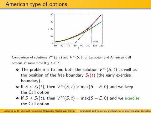
Comparison of solutions V ec(S, t) and V ac (S, t) of European and American Call
options at some time 0 ≤ t < T .
The problem is to find both the solution V ac(S , t) as well asthe position of the free boundary Sf (t) (the early exerciseboundary).
If S < Sf (t), then V ac(S , t) > max(S − E , 0) and we keepthe Call option
If S ≥ Sf (t), then V ac(S , t) = max(S − E , 0) and we exercisethe Call option
Lectures by D. Sevcovic, Comenius University, Bratislava, Slovak republicAnalytical and numerical methods for pricing financial derivatives

American type of options
1 the function V (S , t) is a solution to the Black–Scholes PDE
∂V
∂t+σ2
2S2∂
2V
∂S2+ (r − D)S
∂V
∂S− rV = 0
on a time dependent domain 0 < t < T and 0 < S < Sf (t).
2 The terminal pay–off diagram for the Call option
V (S ,T ) = max(S − E , 0).
3 Boundary conditions for a solution V (S , t) (case of anAmerican Call option)
V (0, t) = 0, V (Sf (t), t) = Sf (t)− E ,∂V
∂S(Sf (t), t) = 1,
at the boundary points S = 0 a S = Sf (t) for 0 < t < T
Lectures by D. Sevcovic, Comenius University, Bratislava, Slovak republicAnalytical and numerical methods for pricing financial derivatives

American type of options
Smooth pasting principle
boundary condition V (Sf (t), t) = Sf (t)− E
represents the continuity of the function V ac(S , t) across thefree boundary Sf (t)
boundary condition ∂V∂S (Sf (t), t) = 1
represents the C 1 continuity of the function V ac(S , t) acrossthe free boundary Sf (t)
The C1 continuity of a solution (smooth pasting principle) can be deduced from theoptimization principle according to which the price of an American option is given by
V ac (S, t) = maxη
V (S, t; η),
where the maximum is taken over the set of all positive smooth functions
η : [0,T ] → R+ and V (S, t; η) is the solution to the Black–Scholes equation on a time
dependent domain 0 < t < T , 0 < S < η(t), and satisfying the terminal pay-off
diagram and Dirichlet boundary conditions V (0, t; η) = 0,V (η(t), t; η) = η(t) − E .
Lectures by D. Sevcovic, Comenius University, Bratislava, Slovak republicAnalytical and numerical methods for pricing financial derivatives

American type of options
0 0.2 0.4 0.6 0.8 1t
160
170
180
190
200S
fHtL
call opciu drzíme
call opciu uplatníme
0 0.2 0.4 0.6 0.8 1t
50
55
60
65
70
75
80
85
SfH
tL
put opciu drzíme
put opciu uplatníme
Behavior of the free boundary Sf (t) (early exercise boundary) for the American Call
(left) and Put (right) option.
For the American Put option we must change:the time dependent domain to 0 < t < T and S > Sf (t);
the terminal pay-off diagram for the Put option V (S,T ) = max(E − S, 0)
boundary conditions
V (+∞, t) = 0, V (Sf (t), t) = E − Sf (t),∂V
∂S(Sf (t), t) = −1,
Lectures by D. Sevcovic, Comenius University, Bratislava, Slovak republicAnalytical and numerical methods for pricing financial derivatives

American type of options
Some recent and so so recent results on the early exercise behavior
According to the paper by Dewynne et al. (1993) andSevcovic (2001) the early exercise behavior of an AmericanCall option close to the expiry T is given by
Sf (t) ≈ K(
1 + 0.638σ√T − t
)
, K = E max(r/D, 1)
According to the paper by Stamicar, Chadam, Sevcovic(1999) the early exercise behavior of an American Put optionclose to the expiry T is given by
Sf (t) = Ee−(r−σ2
2)(T−t)eσ
√2(T−t)η(t) as t → T ,
where η(t) ≈ −√
− ln[2rσ
√
2π(T − t)er(T−t)]
Recently Zhu in papers from 2006, 2007 constructed anexplicit approximation solution to the whole early exerciseboundary problem obtained by the inverse Laplacetransformation.
Lectures by D. Sevcovic, Comenius University, Bratislava, Slovak republicAnalytical and numerical methods for pricing financial derivatives

American type of options
Valuation of American options by a variational inequality
for an American Call option one can show that on the wholedomain 0 < S <∞ and 0 ≤ t < T the following inequalityholds:
L[V ] ≡ ∂V
∂t+σ2
2S2 ∂
2V
∂S2+ (r − D)S
∂V
∂S− rV ≤ 0.
Comparison with the terminal payoff diagram
V (S , t) ≥ V (S ,T ) = max(S − E , 0).
A variational inequality for American Call option
If V (S , t) > max(S − E , 0) ⇒ L[V ](S , t) = 0If V (S , t) = max(S − E , 0) ⇒ L[V ](S , t) < 0
Lectures by D. Sevcovic, Comenius University, Bratislava, Slovak republicAnalytical and numerical methods for pricing financial derivatives
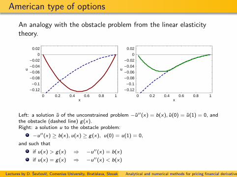
American type of options
An analogy with the obstacle problem from the linear elasticitytheory.
0 0.2 0.4 0.6 0.8 1x
-0.12
-0.1
-0.08
-0.06
-0.04
-0.02
0
0.02
u
0 0.2 0.4 0.6 0.8 1x
-0.12
-0.1
-0.08
-0.06
-0.04
-0.02
0
0.02
u
Left: a solution u of the unconstrained problem −u′′(x) = b(x), u(0) = u(1) = 0, andthe obstacle (dashed line) g(x).Right: a solution u to the obstacle problem:
−u′′(x) ≥ b(x), u(x) ≥ g(x), u(0) = u(1) = 0,
and such that
if u(x) > g(x) ⇒ −u′′(x) = b(x)
if u(x) = g(x) ⇒ −u′′(x) < b(x)
Lectures by D. Sevcovic, Comenius University, Bratislava, Slovak republicAnalytical and numerical methods for pricing financial derivatives

American type of options
Idea of the Project Successive Over Relaxation method
using the transformation V (S , t) = Ee−αx−βτu(x , τ), whereτ = T − t, x = ln(S/E ), leads to the variational inequality
(∂u
∂τ− σ2
2
∂2u
∂x2
)
(u(x , τ)− g(x , τ)) = 0,
∂u
∂τ− σ2
2
∂2u
∂x2≥ 0, u(x , τ)− g(x , τ) ≥ 0
for any x ∈ R, 0 < τ < T .
g(x , τ) = eαx+βτ max(ex − 1, 0) – the transformed pay-offdiagram,
It satisfies the initial condition
u(x , 0) = g(x , 0), for any x ∈ R.
Here: α = r−Dσ2 − 1
2, β = r+D
2+ σ2
8+
(r−D)2
2σ2
Lectures by D. Sevcovic, Comenius University, Bratislava, Slovak republicAnalytical and numerical methods for pricing financial derivatives
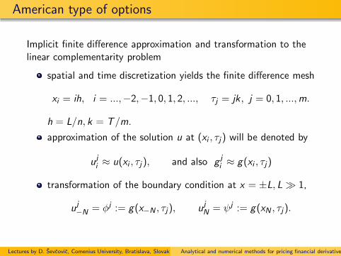
American type of options
Implicit finite difference approximation and transformation to thelinear complementarity problem
spatial and time discretization yields the finite difference mesh
xi = ih, i = ...,−2,−1, 0, 1, 2, ..., τj = jk , j = 0, 1, ...,m.
h = L/n, k = T/m.
approximation of the solution u at (xi , τj) will be denoted by
uji ≈ u(xi , τj ), and also g
ji ≈ g(xi , τj)
transformation of the boundary condition at x = ±L, L ≫ 1,
uj−N = φj := g(x−N , τj), u
jN = ψj := g(xN , τj).
Lectures by D. Sevcovic, Comenius University, Bratislava, Slovak republicAnalytical and numerical methods for pricing financial derivatives

American type of options
The linear complementarity problem for a solution of thediscretized variational inequality can be rewritten as follows:
Auj+1 ≥ uj + bj , uj+1 ≥ g j+1 for each j = 0, 1, ...,m − 1,
(Auj+1 − uj − bj)i (uj+1 − g j+1)i = 0 for each i ,
where u0 = g0. The matrix A is a tridiagonal matrix arising fromthe implicit in time discretization of the parabolic equation∂τu = σ2
2 ∂2xu, i.e.
A =
1 + 2γ −γ 0 · · · 0
−γ 1 + 2γ −γ...
0 · · · 0... −γ 1 + 2γ −γ0 · · · 0 −γ 1 + 2γ
, bj =
γφj+1
0...
0γψj+1
,
where γ = σ2k/(2h2).Lectures by D. Sevcovic, Comenius University, Bratislava, Slovak republicAnalytical and numerical methods for pricing financial derivatives

American type of options
In each time level the goal is to solve linear complementarity
Au ≥ b, u ≥ g ,
(Au − b)i (ui − gi ) = 0 for each i .
We define a recurrent sequence of approximative solution as
u0 = 0, up+1 = max (Tωup + cω, g) for p = 1, 2, ...,
where the maximum is taken component-wisehere Tω is the linear iteration operator arising from theclassical SOR method for the linear problem Au = b. Herecω = ω(D+ ωL)−1b
in terms of vector components, the Projected SOR algorithmreduces to
up+1i = max
[ω
Aii
bi −∑
j<i
Aijup+1j −
∑
j>i
Aijupj
+(1−ω)upi , gi]
where ω ∈ (1, 2) is a relaxation parameter, typically ω ≈ 1.8Lectures by D. Sevcovic, Comenius University, Bratislava, Slovak republicAnalytical and numerical methods for pricing financial derivatives

American type of options
A numerical solution to the problem of valuing American Call andPut options by the Projected Successive Over Relaxation method
30 40 50 60 70 80S
0
5
10
15
20
25
30
35
V
10 20 30 40 50 60 70S
0
10
20
30
40
V
A solution S 7→ V (S , t) of an American Call (left) and Put option(right) obtained by solving the variational inequality by means ofthe Projected SOR (PSOR) algorithm.Dotted curves corresponds to European type of options
Lectures by D. Sevcovic, Comenius University, Bratislava, Slovak republicAnalytical and numerical methods for pricing financial derivatives

American type of options
010
20
S
00.25
0.50.75
1 t
0
5
10
15
V
1020
00.25
0.50.75
010
20S
0 0.25 0.5 0.75 1t
0
5
10
15
V
010
20
0 0.25 0.5 0.75
Two 3D views on the graph of the solution (S , t) 7→ V (S , t) for theprice of the American Call option. Five selected time profiles andcomparison with the terminal pay-off function. One can see theeffect of the smooth pasting of the solution to the pay-off function.
Lectures by D. Sevcovic, Comenius University, Bratislava, Slovak republicAnalytical and numerical methods for pricing financial derivatives

Nonlinear extensions of the Black-Scholes theory
Lecture 8
Modeling transaction costs
Modeling investor’s risk preferences
Jumping volatility model
Risk adjusted pricing methodology model
Numerical approximation scheme
Lectures by D. Sevcovic, Comenius University, Bratislava, Slovak republicAnalytical and numerical methods for pricing financial derivatives

Nonlinear options pricing models
Nonlinear derivative pricing models
Classical Black-Scholes theory does not take into account
Transaction costs (buying or selling assets, bid-ask spreads)
Risk from unprotected (non hedged) portfolio
Other effects
feedback effects on the asset price in the presence of adominant investor
utility function effect of investor’s preferences
Question: how to incorporate both transaction costs and riskarising from a volatile portfolio into the Black-Scholes equationframework?
Lectures by D. Sevcovic, Comenius University, Bratislava, Slovak republicAnalytical and numerical methods for pricing financial derivatives

Transaction costs – Leland model
Leland model for pricing Call and Put options under thepresence of transaction costs
Hoggard, Whaley and Wilmott model - generalization to otheroptions
Volatility σ = σ(∂2SV ) is given by
σ2 = σ2(1− Le sgn(∂2SV ))
where σ > 0 is a constant historical volatility andLe =
√
2/πC/(σ√∆t) is the Leland number where ∆t is time lag
between consecutive transactions
∂V
∂t+ (r − D)S
∂V
∂S+σ2(∂2SV ,S , t)
2S2∂
2V
∂S2− rV = 0
Lectures by D. Sevcovic, Comenius University, Bratislava, Slovak republicAnalytical and numerical methods for pricing financial derivatives

Transaction costs – Leland model
Transaction costs are described following the Hoggard, Whalleyand Wilmott approach (1994) (also referred to as Leland’s model(1985) )
dΠ = dV + δdS − CSk
where
C - the round trip transaction cost per unit dollar oftransaction, C = (Sask − Sbid )/S
k is the number of assets sold or bought during one time lag.Notice that
k ≈ |∆δ| = |∆∂SV | ≈ |∂2SV ||dS |, E (|dW |) =√
2
π
√dt
Lectures by D. Sevcovic, Comenius University, Bratislava, Slovak republicAnalytical and numerical methods for pricing financial derivatives
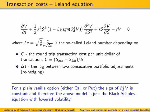
Transaction costs – Leland equation
∂V
∂t+
1
2σ2S2
(1− Le sgn(∂2SV )
) ∂2V
∂S2+ rS
∂V
∂S− rV = 0
where Le =√
2π
C
σ√∆t
is the so-called Leland number depending on
C - the round trip transaction cost per unit dollar oftransaction, C = (Sask − Sbid )/S
∆t - the lag between two consecutive portfolio adjustments(re-hedging)
For a plain vanilla option (either Call or Put) the sign of ∂2SV isconstant and therefore the above model is just the Black-Scholesequation with lowered volatility.
Lectures by D. Sevcovic, Comenius University, Bratislava, Slovak republicAnalytical and numerical methods for pricing financial derivatives

Frey - Stremme model for a large trader
Frey and Stremme (1997) introduced directly the asset pricedynamics in the case when the large trader chooses a givenstock-trading strategy.
Volatility σ = σ(∂2SV ,S) is given by
σ2 = σ2(1− S∂2SV
)−2
where σ2, > 0 are constants.
∂V
∂t+ (r − D)S
∂V
∂S+σ2(∂2SV ,S , t)
2S2∂
2V
∂S2− rV = 0
Lectures by D. Sevcovic, Comenius University, Bratislava, Slovak republicAnalytical and numerical methods for pricing financial derivatives

Barles - Soner model for investor’s utility maximization
If transaction costs are taken into account perfect replicationof the contingent claim is no longer possible
assuming that investor’s preferences are characterized by anexponential utility function Barles and Soner (1998) derived anonlinear Black-Scholes equation
Volatility σ = σ(∂2SV ,S , t) is given by
σ2 = σ2(
1 + Ψ(a2er(T−t)S2∂2SV ))2
where Ψ(x) ≈ (3/2)23 x
13 for x close to the origin. σ2, κ > 0 are
constants.
∂V
∂t+ (r − D)S
∂V
∂S+σ2(∂2SV ,S , t)
2S2∂
2V
∂S2− rV = 0
Lectures by D. Sevcovic, Comenius University, Bratislava, Slovak republicAnalytical and numerical methods for pricing financial derivatives
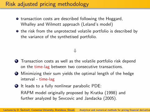
Risk adjusted pricing methodology
transaction costs are described following the Hoggard,Whalley and Wilmott approach (Leland’s model)
the risk from the unprotected volatile portfolio is described bythe variance of the synthetised portfolio.
⇓
1 Transaction costs as well as the volatile portfolio risk dependon the time-lag between two consecutive transactions.
2 Minimizing their sum yields the optimal length of the hedgeinterval - time-lag
3 It leads to a fully nonlinear parabolic PDE:
RAPM model originally proposed by Kratka (1998) andfurther analyzed by Sevcovic and Jandacka (2005).
Lectures by D. Sevcovic, Comenius University, Bratislava, Slovak republicAnalytical and numerical methods for pricing financial derivatives

Transaction costs under δ - hedging
Transaction costs are described following the Hoggard, Whalleyand Wilmott approach (1994)
adopt δ = ∂V∂S hedging
construct a portfolio Π = V − δS donsisting of one optionand δ underlying assets
compare risk part of the portfolio to secure bonds
dΠ = dV + δdS − CSk
r(V − δS)dt = rΠdt = dΠ
where
C - the round trip transaction cost per unit dollar oftransaction, C = (Sask − Sbid )/S
k is the number of assets sold or bought during one time lag.
k ≈ |∆δ| = |∆∂SV | ≈ |∂2SV ||dS |, E (|dW |) =√
2
π
√dt
Lectures by D. Sevcovic, Comenius University, Bratislava, Slovak republicAnalytical and numerical methods for pricing financial derivatives

Modeling transaction costs
∂V
∂t+
1
2σ2S2
(1− Le sgn (∂2SV )
) ∂2V
∂S2+ rS
∂V
∂S− rV = 0
where Le =√
2π
C
σ√∆t
is the so-called Leland number depending on
C - the round trip transaction cost per unit dollar oftransaction, C = (Sask − Sbid )/S
∆t - the lag between two consecutive portfolio adjustments(re-hedging)
For a plain vanilla option (either Call or Put) the sign of ∂2SV isconstant and therefore the above model is just the Black-Scholesequation with lowered volatility.
Lectures by D. Sevcovic, Comenius University, Bratislava, Slovak republicAnalytical and numerical methods for pricing financial derivatives

Risk adjusted pricing methodology model
a portfolio Π consists of options and assets Π = V + δS
is the portfolio Π is highly volatile an investor usually asks fora price compensation.
Volatility of a fluctuating portfolio can be measured by thevariance of relative increments of the replicating portfolio
⇓
introduce the measure rVP of the portfolio volatility risk as follows:
rVP = RVar
(∆ΠS
)
∆t.
Lectures by D. Sevcovic, Comenius University, Bratislava, Slovak republicAnalytical and numerical methods for pricing financial derivatives

Using Ito’s formula the variance of ∆Π can be computed asfollows:
Var(∆Π) = E[(∆Π− E (∆Π))2
]
= E
[(
(∂SV + δ) σSφ√∆t +
1
2σ2S2Γ
(φ2 − 1
)∆t
)2]
.
where φ ≈ N(0, 1) and Γ = ∂2SV .
assuming the δ-hedging of portfolio adjustments, i.e. wechoose δ = −∂SV . For the risk premium rVP we have
rVP =1
2R σ4S2Γ2∆t .
Lectures by D. Sevcovic, Comenius University, Bratislava, Slovak republicAnalytical and numerical methods for pricing financial derivatives

Balance equation for Π = V + δS
dΠ = dV + δdS
dΠ = rΠdt + (rTC + rVP)Sdt
Using Ito’s formula applied to V = V (S , t) and eliminatingstochastic term by taking δ = −∂SV hedge we obtain
∂tV +σ2
2S2∂2SV + rS∂SV − rV = (rTC + rVP)S
where
rTC = C |Γ|σS√2π
1√∆t
is the transaction costs measure
rVP = 12R σ
4S2Γ2∆t is the volatile portfolio risk measure
and Γ = ∂2SV .
Lectures by D. Sevcovic, Comenius University, Bratislava, Slovak republicAnalytical and numerical methods for pricing financial derivatives

Minimizing the total risk in the RAPM model
Total risk rTC + rVP
Dt
rTC+rVP
rTC
rVP
Dt
Tran. costs risk rTC Volatile portfolio risk rVP Total riskrTC + rVP
Both rTC and rVP depend on the time lag ∆t
⇓Minimizing the total risk with respect to the time lag ∆t yields
min∆t
(rTC + rVP) =3
2
(C 2R
2π
) 13
σ2|S∂2SV | 43Lectures by D. Sevcovic, Comenius University, Bratislava, Slovak republicAnalytical and numerical methods for pricing financial derivatives

Nonlinear PDE equation for RAPM
∂tV +1
2σ2S2
(
1− µ(S∂2SV )1/3)
∂2SV + rS∂SV − rV = 0
S > 0, t ∈ (0,T ) whereµ = 3
(C 2R
2π
) 13
fully nonlinear parabolic equation
If µ = 0 (i.e. either R = 0 or C = 0) the equation reduces tothe classical Black-Scholes equation
minus sign in front of µ > 0 corresponds to Bid option priceVbid (price for selling option).
Lectures by D. Sevcovic, Comenius University, Bratislava, Slovak republicAnalytical and numerical methods for pricing financial derivatives

Bid Ask spreads
∂tV +1
2σ2S2
(
1± µ(S∂2SV )1/3)
∂2SV + rS∂SV − rV = 0
A comparison of Bid ( − sign ) and Ask (+ sign) option pricescomputed by means of the RAPM model. The middle dotted lineis the option price computed from the Black-Scholes equation.
22 24 26 28 30S
1
2
3
4
5
6
V
Vbid
Vask
22 24 26 28 30S
1
2
3
4
5
V
Vbid
Vask
Lectures by D. Sevcovic, Comenius University, Bratislava, Slovak republicAnalytical and numerical methods for pricing financial derivatives

RAPM and explanation of volatility smile
Volatility smile phenomenon is non-constant, convex behavior(near expiration price E ) of the implied volatility computed fromclassical Black-Scholes equation.
Volatility smile for DAX index
By RAPM model we can explain the volatility smile analytically.
Lectures by D. Sevcovic, Comenius University, Bratislava, Slovak republicAnalytical and numerical methods for pricing financial derivatives

RAPM and explanation of volatility smile
The Risk adjusted Black-Scholes equation can be viewed as anequation with a variable volatility coefficient
∂tV +σ2(S , t)
2S2∂2SV + rS∂SV − rV = 0
where σ2(S , t) depends on a solution V = V (S , t) as follows:
σ2(S , t) = σ2(
1− µ(S∂2SV (S , t))1/3)
.
Dependence of σ(S , t) on S is depicted in the left for t close to T .The mapping (S , t) 7→ σ(S , t) is shown in the right.
ES
Σ
ΣHS,ΤL
EST
0
t
ΣHS,ΤL
XS
Lectures by D. Sevcovic, Comenius University, Bratislava, Slovak republicAnalytical and numerical methods for pricing financial derivatives

Numerical scheme for quasilinear equation
denote β(H) = σ2
2 (1− µH13 )H
reverse time τ = T − t (time to maturity)
use logarithmic scale x = ln(S/E ) (x ∈ R ↔ S > 0)
introduce new variable H(x , τ) = S∂2SV (S , t)
Then the RAPM equation can be transformed into quasilinearequation
∂τH = ∂2xβ(H) + ∂xβ(H) + r∂xH τ ∈ (0,T ), x ∈ R
Boundary conditions: H(−∞, τ) = H(∞, τ) = 0
Initial condition: H(x , 0) = PDF (d1)
σ√τ∗
d1 =x+(r+σ2
2)τ
σ√τ∗
where
0 < τ∗ << 1 is the switching time.
Lectures by D. Sevcovic, Comenius University, Bratislava, Slovak republicAnalytical and numerical methods for pricing financial derivatives
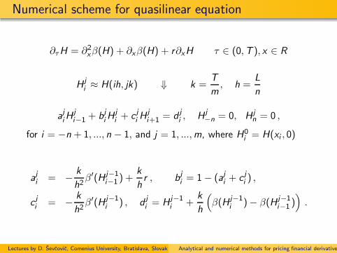
Numerical scheme for quasilinear equation
∂τH = ∂2xβ(H) + ∂xβ(H) + r∂xH τ ∈ (0,T ), x ∈ R
Hji ≈ H(ih, jk) ⇓ k =
T
m, h =
L
n
ajiH
ji−1 + b
jiH
ji + c
ji H
ji+1 = d
ji , H
j−n = 0, H j
n = 0 ,
for i = −n + 1, ..., n − 1, and j = 1, ...,m, where H0i = H(xi , 0)
aji = − k
h2β′(H j−1
i−1 ) +k
hr , b
ji = 1− (aji + c
ji ) ,
cji = − k
h2β′(H j−1
i ) , dji = H
j−1i +
k
h
(
β(H j−1i )− β(H j−1
i−1 ))
.
Lectures by D. Sevcovic, Comenius University, Bratislava, Slovak republicAnalytical and numerical methods for pricing financial derivatives

Calibration of RAPM model
Intra-day behavior of Microsoft stocks (April 4, 2003) and shortlyexpiring Call options with expiry date April 19, 2003. Computedimplied volatilities σRAPM and risk premium coefficients R .
Lectures by D. Sevcovic, Comenius University, Bratislava, Slovak republicAnalytical and numerical methods for pricing financial derivatives

Calibration of RAPM model
One week behavior of Microsoft stocks (March 20 - 27, 2003) andCall options with expiration date April 19, 2003. Computedimplied volatilities σRAPM and risk premiums R .
Lectures by D. Sevcovic, Comenius University, Bratislava, Slovak republicAnalytical and numerical methods for pricing financial derivatives

Jumping volatility nonlinear model
Avellaneda, Levy and Paras proposed a model is to describe optionpricing in incomplete markets where the volatility σ of theunderlying stock process is uncertain but bounded from bellow andabove by given constants σ1 < σ2.
Avellaneda, Levy and Paras nonlinear extension of theBlack–Scholes equation
∂V
∂t+ (r − D)S
∂V
∂S+σ2(∂2SV )
2S2 ∂
2V
∂S2− rV = 0
where the volatility depends on the sign of Γ = ∂2SV
σ2(S2∂2SV ) =
σ21 , if ∂2SV < 0,σ22 , if ∂2SV > 0.
Lectures by D. Sevcovic, Comenius University, Bratislava, Slovak republicAnalytical and numerical methods for pricing financial derivatives
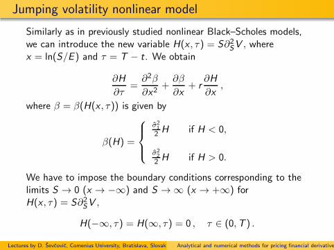
Jumping volatility nonlinear model
Similarly as in previously studied nonlinear Black–Scholes models,we can introduce the new variable H(x , τ) = S∂2SV , wherex = ln(S/E ) and τ = T − t. We obtain
∂H
∂τ=∂2β
∂x2+∂β
∂x+ r
∂H
∂x,
where β = β(H(x , τ)) is given by
β(H) =
σ212 H if H < 0,
σ222 H if H > 0.
We have to impose the boundary conditions corresponding to thelimits S → 0 (x → −∞) and S → ∞ (x → +∞) forH(x , τ) = S∂2SV ,
H(−∞, τ) = H(∞, τ) = 0 , τ ∈ (0,T ) .
Lectures by D. Sevcovic, Comenius University, Bratislava, Slovak republicAnalytical and numerical methods for pricing financial derivatives

Results of numerical approximation of the jumping volatility modelfor the case of the bullish spread.
bullish spread strategy = buying one Call option with exerciseprice E = E1 and selling one Call option with E2 > E1
V (S ,T ) = (S − E1)+ − (S − E2)
+.
in terms of the transformed variable H we have As for theinitial condition we have
H(x , 0) = δ(x − x0)− δ(x − x1), x ∈ R,
where x0 = 0, x1 = ln(E2/E1).
-1 -0.5 0 0.5 1x
-20
0
20
40
60
H
-2 -1 0 1 2x
-0.6
-0.4
-0.2
0
0.2
0.4
H
Plots of the initial approximation of the function H(x , 0) (left) and the solution profile
H(x ,T ) at τ = T (right).
Lectures by D. Sevcovic, Comenius University, Bratislava, Slovak republicAnalytical and numerical methods for pricing financial derivatives
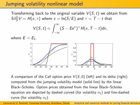
Jumping volatility nonlinear model
Transforming back to the original variable V (S , t) we obtain fromS∂2SV = H(x , τ) where x = ln(S/E ) and τ = T − t that
V (S , t) =
∫ ∞
−∞(S − Eex )+H(x ,T − t)dx ,
where E = E1.
15 20 25 30 35 40 45S
0
1
2
3
4
5
V
10 20 30 40 50 60S
0
0.2
0.4
0.6
0.8
1
D
A comparison of the Call option price V (S , 0) (left) and its delta (right)
computed from the jumping volatility model (solid line) by the linear
Black–Scholes. Option prices obtained from the linear Black–Scholes
equation are depicted by dashed curved (for volatility σ1) and fine-dashed
curve (for volatility σ2).
Lectures by D. Sevcovic, Comenius University, Bratislava, Slovak republicAnalytical and numerical methods for pricing financial derivatives

Interest rate derivatives derivatives
Lecture 9
A stochastic differential equation for modeling the shortinterest rate process
Vasııcek and Cox-Ingersoll–Ross models for the short rateprocess
Interest rate derivatives – zero coupons bonds
Pricing interest rate derivatives by means of a solution to theparabolic partial differential equation
Lectures by D. Sevcovic, Comenius University, Bratislava, Slovak republicAnalytical and numerical methods for pricing financial derivatives

Interest rate derivatives derivatives
Modeling the short rate (overnight) stochastic process
0 2 4 6 8 10 12mesiac
0.03
0.04
0.05
0.06
úro
ková
mie
ra
Daily behavior of the overnight interest rate of BRIBOR in 2007.
modeling the short rate r = r(t) by a solution to a one factorstochastic differential equation
dr = µ(t, r)dt + σ(t, r)dw .
µ(t, r)dt represents a trend or drift of the processσ(t, r) represents a stochastic fluctuation part of the process
Lectures by D. Sevcovic, Comenius University, Bratislava, Slovak republicAnalytical and numerical methods for pricing financial derivatives
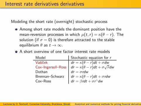
Interest rate derivatives derivatives
Modeling the short rate (overnight) stochastic process
Among short rate models the dominant position have themean-reversion processes in which µ(t, r) = κ(θ − r). Thesolution (if σ = 0) is therefore attracted to the stableequilibrium θ as t → ∞.
A short overview of one factor interest rate models
Model Stochastic equation for rVasıcek dr = κ(θ − r)dt + σdwCox–Ingersoll–Ross dr = κ(θ − r)dt + σ
√rdw
Dothan dr = σrdwBrennan–Schwarz dr = κ(θ − r)dt + σrdwCox–Ross dr = βrdt + σrγdw
Lectures by D. Sevcovic, Comenius University, Bratislava, Slovak republicAnalytical and numerical methods for pricing financial derivatives

Interest rate derivatives derivatives
Modeling the short rate (overnight) stochastic process
Oldrich Alfons Vasıcek, graduated from FJFI and Charles University in Prague
EUROLIBOR Short-rate (overnight) and 1 year interest rates PRIBOR
Lectures by D. Sevcovic, Comenius University, Bratislava, Slovak republicAnalytical and numerical methods for pricing financial derivatives

Interest rate derivatives derivatives
Bond – a derivative of the underlying short rate process
Term structure models describe a functional dependencebetween the time to maturity of a discount bond and itspresent price
Yield of bonds, as a function of maturity, forms the so-calledterm structure of interest rates
If we denote by P = P(t,T ) the price of a bond paying nocoupons at time t with maturity at T then the term structureof yields R(t,T ) is given by
P(t,T ) = e−R(t,T )(T−t), i.e. R(t,T ) = − logP(t,T )
T − t
Lectures by D. Sevcovic, Comenius University, Bratislava, Slovak republicAnalytical and numerical methods for pricing financial derivatives

Interest rate derivatives derivatives
The yield curves R(t,T )
0 2 4 6 8 10 12 14maturita
6.5
6.6
6.7
6.8
6.9vý
nos
AUS
0 2 4 6 8maturita
12
12.5
13
13.5
14
14.5
výno
s
BRA
0 5 10 15 20 25 30maturita
1
1.5
2
2.5
výno
s
JPN
0 5 10 15 20 25 30maturita
4.6
4.7
4.8
4.9
5
výno
s
UK
The term structure (the yield curve) R(t,T ) of governmental bonds in % p.a. fromt =27.5.2008 as a function of the yield R with respect to the time to maturity T − t.
Australia, Brazil, Japan United Kingdom.
Lectures by D. Sevcovic, Comenius University, Bratislava, Slovak republicAnalytical and numerical methods for pricing financial derivatives
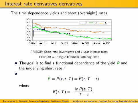
Interest rate derivatives derivatives
The time dependence yields and short (overnight) rates
PRIBOR: Short-rate (overnight) and 1 year interest rates
PRIBOR = PRague Interbank Offering Rate
The goal is to find a functional dependence of the yield R andthe underlying short rate r
P = P(r , t,T ) = P(r ,T − t)
where
R(t,T ) = − lnP(t,T )
T − t.
Lectures by D. Sevcovic, Comenius University, Bratislava, Slovak republicAnalytical and numerical methods for pricing financial derivatives

Interest rate derivatives derivatives
Modeling the bond price by a solution to a PDE
Suppose that the underlying short rate process follows theSDE:
dr = µ(t, r)dt + σ(t, r)dw .
for the Vasıcek model: dr = κ(θ − r)dt + σdwfor the Cox–Ingersoll–Ross model: dr = κ(θ − r)dt + σ
√rdw
Suppose that the price of a zero coupon bond P is a smoothfunction P = P(r , t,T ) of the short rate r , actual time t andthe maturity time T (t < T ).by Ito’s lemma we have
dP =
(∂P
∂t+ µ
∂P
∂r+σ2
2
∂2P
∂r2
)
︸ ︷︷ ︸
µB (t,r)
dt + σ∂P
∂r︸ ︷︷ ︸
σB (t,r)
dw
where µB(r , t) and σB(r , t) stand for the drift and volatility ofthe bond price
Lectures by D. Sevcovic, Comenius University, Bratislava, Slovak republicAnalytical and numerical methods for pricing financial derivatives

Interest rate derivatives derivatives
Modeling the bond price by a solution to a PDE
Construct a portfolio from two bonds with two differentmaturities T1 and T2
It consits of one bond with maturity T1 and ∆ – bonds withmaturity T2
Its value is therefore π = P(r , t,T1) + ∆P(r , t,T2)
the change of the portfolio dπ is equal to:
dπ = dP(r , t,T1) + ∆dP(r , t,T2)
= (µB(r , t,T1) + ∆µB(r , t,T2)) dt
+(σB(r , t,T1) + ∆σB(r , t,T2)) dw .
Lectures by D. Sevcovic, Comenius University, Bratislava, Slovak republicAnalytical and numerical methods for pricing financial derivatives

Interest rate derivatives derivatives
Modeling the bond price by a solution to a PDE
similarly as in the case of options our goal is to eliminate thevolatile (fluctuating) part of the portfolio of bonds (tenor)
it can be accomplished by taking
∆ = −σB(t, r ,T1)
σB(t, r ,T2)
then the differential of the risk-neutral portfolio of bonds(tenor)
dπ =
(
µB(t, r ,T1)−σB(t, r ,T1)
σB(t, r ,T2)µB(t, r ,T2)
)
dt.
to avoid the possibility of arbitrage the yield of the portfolioshould be equal to the risk-less short interest rate r , i.e.dπ = rπdt. Therefore
µB(t, r ,T1)−σB(t, r ,T1)
σB(t, r ,T2)µB(t, r ,T2) = rπ .
Lectures by D. Sevcovic, Comenius University, Bratislava, Slovak republicAnalytical and numerical methods for pricing financial derivatives
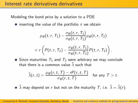
Interest rate derivatives derivatives
Modeling the bond price by a solution to a PDE
inserting the value of the portfolio π we obtain
µB(t, r ,T1)−σB(t, r ,T1)
σB(t, r ,T2)µB(t, r ,T2)
= r
(
P(t, r ,T1)−σB(t, r ,T1)
σB(t, r ,T2)P(t, r ,T2)
)
.
Since maturities T1 and T2 were arbitrary we may concludethat there is a common value λ such that
λ(r , t) =µB(r , t,T )− rP(r , t,T )
σB(r , t,T )for any T > t.
λ may depend on r but not on the maturity T , i.e. λ = λ(r).
Lectures by D. Sevcovic, Comenius University, Bratislava, Slovak republicAnalytical and numerical methods for pricing financial derivatives

Interest rate derivatives derivatives
Modeling the bond price by a solution to a PDE
ReCall that
µB(t, r) =∂P
∂t+ µ
∂P
∂r+σ2
2
∂2P
∂r2
σB(t, r) = σ∂P
∂r
where we supposed that the underlying short rate processfollows the SDE: dr = µ(t, r)dt + σ(t, r)dw .
In summary, we can deduce the parabolic PDE for the zerocoupon bond price
∂P
∂t+ (µ(r , t)− λ(r , t)σ(r , t))
∂P
∂r+σ2(r , t)
2
∂2P
∂r2− rP = 0.
At the maturity t = T the price of the bond is prescribed andit is independent of the short rate r , i.e.
P(r ,T ,T ) = 1 for any r > 0.
Lectures by D. Sevcovic, Comenius University, Bratislava, Slovak republicAnalytical and numerical methods for pricing financial derivatives

Interest rate derivatives derivatives
Modeling the bond price by a solution to a PDE
for the Vasıcek model where dr = κ(θ − r)dt + σdw we takeλ(r , t) ≡ λ and we obtain the PDE:
−∂P∂τ
+ (κ(θ − r)− λσ)∂P
∂r+σ2
2
∂P
∂r2− rP = 0
for the Cox–Ingersoll–Ross model wheredr = κ(θ − r)dt + σ
√rdw we take λ(r , t) = λ
√r and we
obtain the PDE:
−∂P∂τ
+ (κ(θ − r)− λσr)∂P
∂r+σ2
2r∂2P
∂r2− rP = 0,
In both models τ = T − t stands for the time remaining tomaturity of the bond
Lectures by D. Sevcovic, Comenius University, Bratislava, Slovak republicAnalytical and numerical methods for pricing financial derivatives

Interest rate derivatives derivatives
An explicit solution for the Cox–Ingersoll–Ross model
construct a solution in the form P(r , τ) = A(τ)e−B(τ)r
inserting this ansatz into the CIR equation and comparing theterms of the order 1 and r we obtain
A+ κθAB = 0,
B + (κ+ λσ)B +σ2
2B2 − 1 = 0,
functions A, B satisfy initial conditions A(0) = 1, B(0) = 0the explicit solution to the system of ODEs for A,B is:
B(τ) =2(eφτ − 1
)
(ψ + φ) (eφτ − 1) + 2φ,
A(τ) =
(
2φe(φ+ψ)τ/2
(φ+ ψ)(eφτ − 1) + 2φ
) 2κθσ2
,
where ψ = κ+ λσ, φ =√
ψ2 + 2σ2 =√
(κ+ λσ)2 + 2σ2.
Lectures by D. Sevcovic, Comenius University, Bratislava, Slovak republicAnalytical and numerical methods for pricing financial derivatives

Interest rate derivatives derivatives
An explicit solution for the Vasıcek model
construct a solution in the form P(r , τ) = A(τ)e−B(τ)r
one can construct an analogous system of ODEs for functionsA,B
the explicit solution of the system of ODEs yields:
B(τ) =1− e−κτ
κ,
lnA(τ) =
[1
κ(1− e−κτ )− τ
]
R∞ − σ2
4κ3(1− e−κτ )2,
where R∞ = θ − λσκ − σ2
2κ2.
Lectures by D. Sevcovic, Comenius University, Bratislava, Slovak republicAnalytical and numerical methods for pricing financial derivatives

Interest rate derivatives derivatives
An explicit solution for the Vasıcek model
0 0.1 0.2 0.3 0.4 0.5T
0.035
0.04
0.045
0.05
R
0 0.1 0.2 0.3 0.4 0.5T
0.035
0.04
0.045
0.05
R
The term structure of interest rates R(r , t,T ) on bonds computed by the Vasıcek
model for two different values of the short rate r (r = 0.03 and r = 0.05) at given
time t < T .
Lectures by D. Sevcovic, Comenius University, Bratislava, Slovak republicAnalytical and numerical methods for pricing financial derivatives
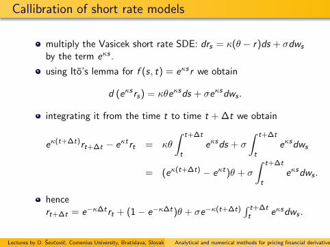
Callibration of short rate models
multiply the Vasicek short rate SDE: drs = κ(θ − r)ds + σdws
by the term eκs .
using Ito’s lemma for f (s, t) = eκs r we obtain
d (eκsrs) = κθeκsds + σeκsdws .
integrating it from the time t to time t +∆t we obtain
eκ(t+∆t)rt+∆t − eκtrt = κθ
∫ t+∆t
t
eκsds + σ
∫ t+∆t
t
eκsdws
= (eκ(t+∆t) − eκt)θ + σ
∫ t+∆t
t
eκsdws .
hencert+∆t = e−κ∆trt + (1− e−κ∆t)θ + σe−κ(t+∆t)
∫ t+∆t
teκsdws .
Lectures by D. Sevcovic, Comenius University, Bratislava, Slovak republicAnalytical and numerical methods for pricing financial derivatives

Callibration of short rate models
The conditional distribution rt+∆t conditioned to the state rtat time t is a normal distribution
E (rt+∆t |rt) = e−κ∆trt + (1− e−κ∆t)θ,
Var(rt+∆t |rt) = σ2e−2κ(t+∆t)Var
(∫ t+∆t
t
eκsdws
)
= σ2e−2κ(t+∆t)E
([∫ t+∆t
t
eκsdws
]2)
= σ2e−2κ(t+∆t)
∫ t+∆t
t
(eκs)2 ds =σ2
2κ(1− e−2κ∆t)
using Ito’s isometry
We obtain
rt+∆t |rt ∼ N
(
e−κ∆trt +(
1− e−κ∆t)
θ,σ2
2κ
(
1− e−2κ∆t))
.
Lectures by D. Sevcovic, Comenius University, Bratislava, Slovak republicAnalytical and numerical methods for pricing financial derivatives

Callibration of short rate models
let the statistical data for the short rate are given:r0, r∆t , . . . , rN∆t evaluated at times: 0,∆t, . . . ,N∆t.
define
ν2t =σ2
2κ
(
1− e−2κ∆t)
, εt = rt−θ(
1− e−κ∆t)
−e−κ∆trt−∆t .
εt/νt ∈ N(0, 1) are IID residuals
the likelihood function L = L(κ, θ, σ2) of the random vector εis a product of normal distributions, i.e.
L = ΠN∆t=1∆f (εt ;κ, θ, σ
2), f (εt ;κ, θ, σ2) =
1√
2πν2te− ε2t
2ν2t
the logarithm of likelihood function L can be written as
lnL = −1
2
N∑
t=1
ln ν2t +ε2tν2t.
maximizing this function we obtain the estimates of κ, θ, σ2.
Lectures by D. Sevcovic, Comenius University, Bratislava, Slovak republicAnalytical and numerical methods for pricing financial derivatives

Black–Scholes model for pricing financial derivatives
Appendix
Stochastic differential calculus
Density distribution function and the Fokker–Planck equation
Multidimensional extension of Ito’s lemma
Lectures by D. Sevcovic, Comenius University, Bratislava, Slovak republicAnalytical and numerical methods for pricing financial derivatives

Ito’s lemma and Fokker–Planck equation
Suppose that a process x(t), t ≥ 0 follows a SDE (It0’sprocess)
dx = µ(x , t)dt + σ(x , t)dW ,
where µ a drift function and σ is a volatility of the process.
Denote by
G = G (x , t) = P(x(t) < x | x(0) = x0)
the conditional probability distribution function of the processx(t), t ≥ 0 starting almost surely from the initial conditionx0.
Then the cumulative distribution function G can be computedfrom its density function g = ∂G/∂x where g(x , t) is asolution to the Fokker–Planck equation:
∂g
∂t=
1
2
∂2
∂x2(σ2g
)− ∂
∂x(µg) , g(x , 0) = δ(x − x0).
Lectures by D. Sevcovic, Comenius University, Bratislava, Slovak republicAnalytical and numerical methods for pricing financial derivatives

Ito’s lemma and Fokker–Planck equation
Here δ(x − x0) is the Dirac function with support at x0. It means:
δ(x − x0) =
0 if x 6= x0,
+∞ if x = x0and
∫ ∞
−∞δ(x − x0)dx = 1.
In our case we have, at the origin t = 0,
G (x , 0) =
∫ x
−∞δ(ξ − x0)dξ =
0 if x < x0,1 if x ≥ x0,
so the process x(t), t ≥ 0 at t = 0 is almost surely equal to x0.
Lectures by D. Sevcovic, Comenius University, Bratislava, Slovak republicAnalytical and numerical methods for pricing financial derivatives
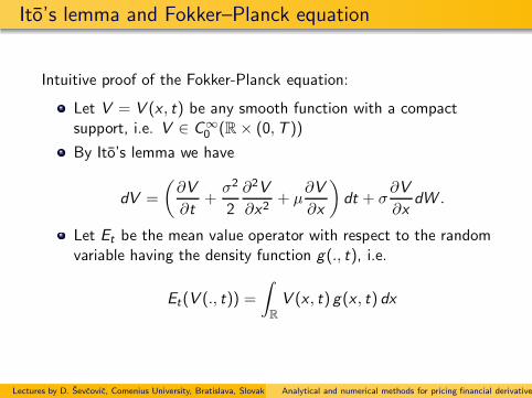
Ito’s lemma and Fokker–Planck equation
Intuitive proof of the Fokker-Planck equation:
Let V = V (x , t) be any smooth function with a compactsupport, i.e. V ∈ C∞
0 (R× (0,T ))
By Ito’s lemma we have
dV =
(∂V
∂t+σ2
2
∂2V
∂x2+ µ
∂V
∂x
)
dt + σ∂V
∂xdW .
Let Et be the mean value operator with respect to the randomvariable having the density function g(., t), i.e.
Et(V (., t)) =
∫
R
V (x , t) g(x , t) dx
Lectures by D. Sevcovic, Comenius University, Bratislava, Slovak republicAnalytical and numerical methods for pricing financial derivatives
Ito’s lemma and Fokker–Planck equation
Then
dEt(V (., t)) = Et(dV (., t)) = Et
(∂V
∂t+σ2
2
∂2V
∂x2+ µ
∂V
∂x
)
dt.
because random variables σ(., t)∂V∂x (., t) and dW (t) areindependent and E(dW (t)) = 0. Therefore
Et
(
σ(., t)∂V
∂x(., t)dW (t)
)
= 0
Lectures by D. Sevcovic, Comenius University, Bratislava, Slovak republicAnalytical and numerical methods for pricing financial derivatives

Ito’s lemma and Fokker–Planck equation
Since V ∈ C∞0 we have V (x , 0) = V (x ,T ) = 0 and
V (x , t) = 0 for |x | > R , where R > 0 is sufficiently large.
By integration by parts we obtain
0 =
∫ T
0
d
dtEt(V (., t))dt =
∫ T
0Et
(∂V
∂t+σ2
2
∂2V
∂x2+ µ
∂V
∂x
)
dt
=
∫ T
0
∫
R
(∂V
∂t+σ2
2
∂2V
∂x2+ µ
∂V
∂x
)
g(x , t) dx dt
=
∫ T
0
∫
R
V (x , t)
(
−∂g∂t
+1
2
∂2
∂x2(σ2g
)− ∂
∂x(µg)
)
dx dt.
Since V ∈ C∞0 (R × (0,T )) is an arbitrary function we obtain
the Fokker–Planck equation for the density g = g(x , t):
−∂g∂t
+1
2
∂2
∂x2(σ2g
)− ∂
∂x(µg) = 0, x ∈ R, t > 0,
g(x , 0) = δ(x − x0), x ∈ R.
Lectures by D. Sevcovic, Comenius University, Bratislava, Slovak republicAnalytical and numerical methods for pricing financial derivatives

Ito’s lemma and Fokker–Planck equation
Example: dx = dW and x(0) = 0 a.s.It means x(t) is a Wiener process
The Fokker–Planck (diffusion) equation reads as follows:
∂g
∂t− 1
2
∂2g
∂x2= 0, x ∈ R, t > 0,
Its solution (normalized to be a probabilistic density)
g(x , t) =1√2πt
e−x2
2t
is indeed a density function of the normal random variableW (t) ∼ N(0, t)
Lectures by D. Sevcovic, Comenius University, Bratislava, Slovak republicAnalytical and numerical methods for pricing financial derivatives

Ito’s lemma and Fokker–Planck equation
Example: dr = κ(θ − r)dt + σdW and and r(0) = r0.This is the so-called Ornstein-Uhlenbeck mean reversionprocess used arising the modeling of the the rate interest ratestochastic process r(t), t ≥ 0.The Fokker–Planck equation reads as follows:
∂f
∂t=σ2
2
∂2f
∂r2− ∂
∂r(κ(θ − r)f )
Its solution (normalized to be a probabilistic density function)
f (r , t) =1
√
2πσ2te− (r−rt )
2
2σ2t
is the density function for the normal random variabler(t) ∼ N(rt , σ
2t ) satisfying the above SDE. Here
rt = θ(1− e−κt) + r0e−κt , σ2t =
σ2
2κ(1− e−2κt).
Lectures by D. Sevcovic, Comenius University, Bratislava, Slovak republicAnalytical and numerical methods for pricing financial derivatives

Ito’s lemma and Fokker–Planck equation
Simulation of the process r(t) satisfying dr = κ(θ − r)dt + σdW and
r(0) = r0 = 0.08. Here θ = 0.04.
Time steps of the evolution of the density function f (r , t) for various times t.
The process r(t) started from r0 = 0.02. The limiting value θ = 0.04.
0 0.01 0.02 0.03 0.04 0.05 0.06 0.07r
0
20
40
60
frek
venc
ia
Θr0
Shift of the density function f (r , t)is due to the drift in the F-P equation
∂f
∂t=σ2
2
∂2f
∂r2− ∂
∂r(κ(θ − r)f )
Lectures by D. Sevcovic, Comenius University, Bratislava, Slovak republicAnalytical and numerical methods for pricing financial derivatives

Multidimensional Ito’s lemma
Multidimensional stochastic processes
dxi = µi (~x , t)dt +
n∑
k=1
σik(~x , t)dwk ,
where ~w = (w1,w2, ...,wn)T is a vector of Wiener processes
having mutually independent increments
E(dwi dwj) = 0 for i 6= j , E((dwi )2) = dt .
It can be rewritten in a vector form
d~x = ~µ(~x , t)dt + K (~x , t)d ~w ,
where ~x = (x1, x2, ..., xn)T and K is an n × n matrix
K (~x , t) = (σij(~x , t))i ,j=1,...,n.
Lectures by D. Sevcovic, Comenius University, Bratislava, Slovak republicAnalytical and numerical methods for pricing financial derivatives

Multidimensional Ito’s lemma
Expanding a smooth functionf = f (~x , t) = f (x1, x2, ..., xn, t) : R
n × [0,T ] → R into thesecond order Taylor series yields:
df =∂f
∂tdt +∇x f .d~x
+1
2
(
(d~x)T∇2x f d~x + 2
∂f
∂t.∇x fd~x dt +
∂2f
∂t2(dt)2
)
+ h.o.t.
The term (d~x)T∇2x f d~x =
∑ni ,j=1
∂2f∂xi∂xj
dxi dxj can be
expanded using the relation between processes xi and xj
dxi dxj =n∑
k,l=1
σikσjldwk dwl + O((dt)3/2) + O((dt)2)
≈ (
n∑
k=1
σikσjk)dt + O((dt)3/2) +O((dt)2) as dt → 0.
Lectures by D. Sevcovic, Comenius University, Bratislava, Slovak republicAnalytical and numerical methods for pricing financial derivatives

Multidimensional Ito’s lemma
The multidimensional Ito’s lemma gives the SDE for thecomposite function f = f (~x , t) in the form:
df =
(∂f
∂t+
1
2K : ∇2
x f K
)
dt +∇x f d~x
where
K : ∇2x f K =
n∑
i ,j=1
∂2f
∂xi∂xj
n∑
k=1
σikσjk
Lectures by D. Sevcovic, Comenius University, Bratislava, Slovak republicAnalytical and numerical methods for pricing financial derivatives

Multidimensional Ito’s lemma and Fokker-Planck equation
By following the same procedure of as in the scalar case weobtain, for the joint density distribution functiong(x1, x2, ..., xn, t),
g(x1, x2, ..., xn, t) = P(x1(t) = x1, x2(t) = x2, ..., xn(t) = xn, t)
conditioned to the initial condition statex1(0) = x01 , x2(0) = x02 , ..., xn(0) = x0n that:
∂g
∂t+ div(~µg) =
1
2
n∑
i ,j=1
n∑
k=1
σikσjk∂2g
∂xi∂xj
g(~x , 0) = δ(~x − ~x0),
Fokker–Planck equation in the multidimensional case
Lectures by D. Sevcovic, Comenius University, Bratislava, Slovak republicAnalytical and numerical methods for pricing financial derivatives

Multidimensional Ito’s lemma and Fokker-Planck equation
Example: The multidimensional Fokker–Planck equation for asystem of uncorrelated SDE’s
dx1 = µ1(~x , t)dt + σ1dw1
dx2 = µ2(~x , t)dt + σ2dw2
......
...
dxn = µn(~x , t)dt + σndwn
with mutually independent increments of Wiener processes
E(dwi dwj) = 0 for i 6= j , E((dwi )2) = dt .
The Fokker–Planck equations reads as follows:
∂g
∂t+ div(~µg) =
1
2
n∑
i=1
∂2
∂x2i
(σ2i g
)
This is a scalar parabolic reaction–diffusion equation for g
Lectures by D. Sevcovic, Comenius University, Bratislava, Slovak republicAnalytical and numerical methods for pricing financial derivatives
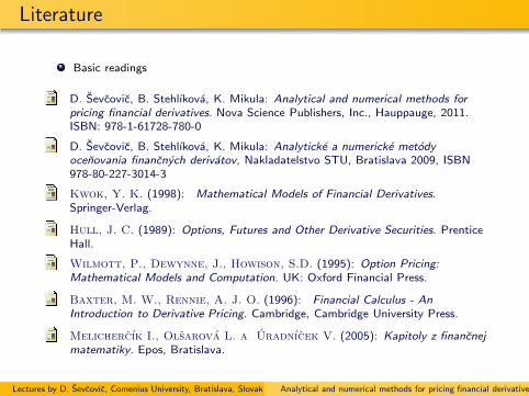
Literature
Basic readings
D. Sevcovic, B. Stehlıkova, K. Mikula: Analytical and numerical methods for
pricing financial derivatives. Nova Science Publishers, Inc., Hauppauge, 2011.ISBN: 978-1-61728-780-0
D. Sevcovic, B. Stehlıkova, K. Mikula: Analyticke a numericke metody
ocenovania financnych derivatov, Nakladatelstvo STU, Bratislava 2009, ISBN978-80-227-3014-3
Kwok, Y. K. (1998): Mathematical Models of Financial Derivatives.Springer-Verlag.
Hull, J. C. (1989): Options, Futures and Other Derivative Securities. PrenticeHall.
Wilmott, P., Dewynne, J., Howison, S.D. (1995): Option Pricing:
Mathematical Models and Computation. UK: Oxford Financial Press.
Baxter, M. W., Rennie, A. J. O. (1996): Financial Calculus - An
Introduction to Derivative Pricing. Cambridge, Cambridge University Press.
Melichercık I., Olsarova L. a Uradnıcek V. (2005): Kapitoly z financnej
matematiky. Epos, Bratislava.
Lectures by D. Sevcovic, Comenius University, Bratislava, Slovak republicAnalytical and numerical methods for pricing financial derivatives
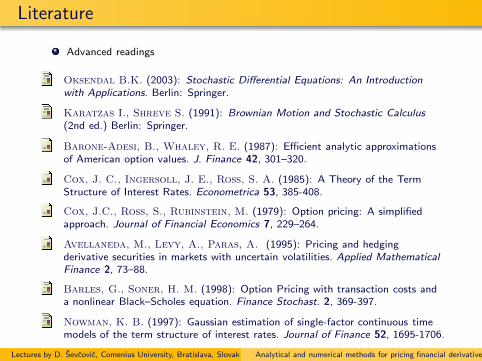
Literature
Advanced readings
Oksendal B.K. (2003): Stochastic Differential Equations: An Introduction
with Applications. Berlin: Springer.
Karatzas I., Shreve S. (1991): Brownian Motion and Stochastic Calculus
(2nd ed.) Berlin: Springer.
Barone-Adesi, B., Whaley, R. E. (1987): Efficient analytic approximationsof American option values. J. Finance 42, 301–320.
Cox, J. C., Ingersoll, J. E., Ross, S. A. (1985): A Theory of the TermStructure of Interest Rates. Econometrica 53, 385-408.
Cox, J.C., Ross, S., Rubinstein, M. (1979): Option pricing: A simplifiedapproach. Journal of Financial Economics 7, 229–264.
Avellaneda, M., Levy, A., Paras, A. (1995): Pricing and hedgingderivative securities in markets with uncertain volatilities. Applied Mathematical
Finance 2, 73–88.
Barles, G., Soner, H. M. (1998): Option Pricing with transaction costs anda nonlinear Black–Scholes equation. Finance Stochast. 2, 369-397.
Nowman, K. B. (1997): Gaussian estimation of single-factor continuous timemodels of the term structure of interest rates. Journal of Finance 52, 1695-1706.
Lectures by D. Sevcovic, Comenius University, Bratislava, Slovak republicAnalytical and numerical methods for pricing financial derivatives

Literature
Advanced readings
Vasıcek, O. A. (1977): An Equilibrium Characterization of the Term Structure.Journal of Financial Economics 5, 177-188.
Dewynne, J. N., Howison, S. D., Rupf, J., Wilmott, P. (1993): Somemathematical results in the pricing of American options. Euro. J. Appl. Math. 4,381–398.
Fong, H. G., Vasıcek, O. A. (1991): Fixed-Income Volatility Management.Journal of Portfolio Management (Summer), 41-46.
Zhu, S.P. (2006): A new analytical approximation formula for the optimalexercise boundary of American put options. International Journal of Theoreticaland Applied Finance 9, 1141–1177.
Papanicolaou, G.C. (1973): Stochastic Equations and Their Aplications.American Mathematical Monthly 80, 526 - 545.
Stamicar, R., Sevcovic, D.. Chadam, J. (1999): The early exercise boundaryfor the American Put near expiry: numerical approximation. Canad. Appl. Math.
Quarterly 7, 427–444.
Sevcovic, D. (2001): Analysis of the free boundary for the pricing of anAmerican Call option. Euro. Journal on Applied Mathematics 12, 25–37.
Lectures by D. Sevcovic, Comenius University, Bratislava, Slovak republicAnalytical and numerical methods for pricing financial derivatives

Literature
Advanced readings
Ho T.S.Y., Lee S.B. (1986): Term structure movements and pricing interestrate contingent claims. Journal of Finance 41 1011–1029.
Hoggard, T., Whalley, A. E., Wilmott, P. (1994): Hedging optionportfolios in the presence of transaction costs. Advances in Futures and Options
Research 7, 21–35.
Chadam, J. (2008): Free Boundary Problems in Mathematical Finance. Progressin Industrial Mathematics at ECMI 2006, Vol. 12, Springer Berlin Heidelberg.
Chan, K. C., Karolyi, G. A., Longstaff, F. A., Sanders, A. B. (1992):An Empirical Comparison of Alternative Models of the Short-Term Interest Rate.The Journal of Finance 47, 1209-1227.
Jandacka , M., Sevcovic, D. (2005): On the risk adjusted pricingmethodology based valuation of vanilla options and explanation of the volatilitysmile. Journal of Applied Mathematics 3, 235–258.
Johnson, H. (1983): An analytic approximation of the American Put price. J.Finan. Quant. Anal. 18, 141–148.
Karatzas, I. (1988): On the pricing American options. Appl. Math. Optim. 17,37–60.
Kratka, M. (1998): No Mystery Behind the Smile. Risk 9, 67–71.
Lectures by D. Sevcovic, Comenius University, Bratislava, Slovak republicAnalytical and numerical methods for pricing financial derivatives

Download
The lecture slides are available for download fromwww.iam.fmph.uniba.sk/institute/sevcovic/slides-hitotsubashi/
Lectures by D. Sevcovic, Comenius University, Bratislava, Slovak republicAnalytical and numerical methods for pricing financial derivatives